Quasinormal modes of Kerr-de Sitter black holes via the Heun function

Abstract

This note addresses quasinormal mode frequencies of four-dimensional asymptotically de Sitter rotating black holes. The main motivation is that Mathematica 12.1 has implemented a new family of special functions: Heun functions. Using the fact that Teukolsky’s equations for Kerr-de Sitter black holes are mapped to Heun’s equations, we are able to compute their quasinormal mode frequencies by the Heun function. In this approach, Mathematica normally evaluates these frequencies to arbitrary numerical precision in a few seconds. We further discuss an application to asymptotically flat rotating black holes.

1 Motivations

Recently, Mathematica has implemented a new class of special functions, known as Heun functions zotero-803 . The Heun function is a solution to Heun’s differential equation:

$$y^{\prime\prime}(z)+\left(\frac{\gamma}{z}+\frac{\delta}{z-1}+\frac{\epsilon}{z-a}\right)y^{\prime}(z)+\frac{\alpha\beta z-q}{z(z-1)(z-a)}y(z)=0,$$ (1)

where $\gamma+\delta+\epsilon=\alpha+\beta+1$. Heun’s equation is a second order Fuchsian differential equation with four singular points ronveaux1995 ; kristensson2010 ; zotero-804 . The Heun function is a generalization of the Gauss hypergeometric function, but has some significant differences. For instance, it has an additional parameter $q$, called an accessory parameter, which does not affect the charcteristic exponents at any singular point. Since the Heun function is much less familiar than the hypergeometric function, Mathematica did not have it for a long time.

Motivated by this great update, we apply this special function to black hole physics. For other possible applications, see birkandan2017 ; hortacsu2018a for instance. The idea is very simple. It is known that both angular and radial Teukolsky equations teukolsky1972 for Kerr (anti-)de Sitter black holes are mapped to Heun’s differential equations suzuki1998 . Their solutions are expressed by the Heun function. Using them, we compute quasinormal mode (QNM) frequencies as well as generalized spin-weighted spheroidal eigenvalues.

The QNM problem for the Kerr-(A)dS₄ black holes has a great advantage. Since all the singular points in Heun’s equation are regular, these are all equivalent. If one constructs local solutions at a certain singular point, one can use them in the construction of local solutions at the other singular points by symmetry. In fact, it is well-known that all the local solutions in Heun’s equation can be expressed in terms of the same (local) Heun function, as is so in the hypergeometric differential equation. This nice property, however, is lost if one considers asymptotically flat geometries. In these cases, two regular singular points get confluent, and result in an irregular singular point. Connection problems between a regular singular point and an irregular singular point are more difficult in general. One needs to modify the argument here for such problems fiziev2006 ; fiziev2010 . We will be back to this issue in the concluding section.

We explicitly construct local solutions to the Teukolsky equation for the Kerr-dS₄ black holes, and use them to determine the QNM frequencies. We use the standard Wronskian method to do so. It is easy to put all the computations on Mathematica, and our simple program provides the QNM frequencies very rapidly (in a few seconds) and precisely (up to any digits). We do them for the Schwarzschild-dS and Kerr-dS cases. All the obtained results are consistent with available data in the literature.

Implementation.

The reader finds a sample Mathematica notebook in arXiv. This program works only in Mathematica 12.1 (or later). All the numerical data in this note are simply generated by this program.

2 From Teukolsky to Heun

Since our purpose is merely to show an efficiency of the Heun function in Mathematica, we do not discuss perturbations of the Kerr-(A)dS black holes. We start our argument with the Teukolsky equation for such black holes khanal1983 ; chambers1994 ; suzuki1998 . The Kerr-(A)dS₄ black holes have three independent parameters: mass $M$, angular momentum per unit mass $a$ and the cosmological constant $\Lambda$. For later convenience, we define a new parameter by

$$\alpha=\frac{\Lambda a^{2}}{3}.$$ (2)

To fix our convention, let us write the metric of the Kerr-(A)dS₄ black holes in the Boyer-Lindquist coordinates:

$$ds^{2}=-\frac{\Delta_{r}}{(1+\alpha)^{2}\rho^{2}}(dt-a\sin^{2}\theta d\phi)^{2}+\frac{\Delta_{\theta}\sin^{2}\theta}{(1+\alpha)^{2}\rho^{2}}[adt-(r^{2}+a^{2})d\phi]^{2}+\frac{\rho^{2}}{\Delta_{r}}dr^{2}+\frac{\rho^{2}}{\Delta_{\theta}}d\theta^{2},$$ (3)

where $\rho^{2}=r^{2}+a^{2}\cos^{2}\theta$ and

$$\Delta_{r}=(r^{2}+a^{2})\left(1-\frac{\Lambda}{3}r^{2}\right)-2Mr,\qquad\Delta_{\theta}=1+\alpha\cos^{2}\theta.$$ (4)

2.1 Angular part

We basically follow the convention in suzuki1998 . The Teukolsky equation is separated into the angular and the radial equations. The angular Teukolsky equation is given by eq. (3.1) in suzuki1998 . We rewrite it as a more compact form:

$$\biggl{[}\frac{d}{dx}(1+\alpha x^{2})(1-x^{2})\frac{d}{dx}+\lambda-s(1-\alpha)-2\alpha x^{2}$$ (5)

$$\quad+\frac{(1+\alpha)^{2}}{1+\alpha x^{2}}\biggl{(}c^{2}x^{2}-2csx-c^{2}+2cm+\frac{4\alpha}{1+\alpha}smx-\frac{(m+sx)^{2}}{1-x^{2}}\biggr{)}\biggr{]}S(x)=0,$$

where $x=\cos\theta$, $s$ is a spin-weight of a perturbing field, $m$ is an azimuthal number and $c=a\omega$ with frequency $\omega$. $\lambda$ is a separation constant, which is determined by a requirement of the regularity for $S(x)$ both at $x=\pm 1$. We will show that this two-point boundary value problem is solved by the Heun function.

In the flat limit $\Lambda\to 0$ (i.e., $\alpha\to 0$), the angular equation (5) reduces to the so-called spin-weighted spheroidal equation teukolsky1972 . The relation to the original separation constant $A$ in teukolsky1972 is $\lambda|_{\alpha=0}=A+2s-2cm+c^{2}$. Even in this case, the eigenvalue is not known analytically. If taking a further limit $a\to 0$, then $\lambda\to\ell(\ell+1)-s(s-1)$ with multipole number $\ell$.

If we take the spinless limit $a\to 0$ first with $\omega$ and $\Lambda$ fixed (i.e., $c\to 0$ and $\alpha\to 0$), then the reduced equation does not contain $\Lambda$. Therefore we conclude $\lambda|_{a=0}=\ell(\ell+1)-s(s-1)$.

At first glance, the differential equation (5) has five regular singular points at $x=\pm 1,\pm i/\sqrt{\alpha},\infty$. However the infinity point turns out to be a removable singularity. Its characteristic exponents are $-1$ and $0$, and moreover the corresponding two Frobenius solutions have no logarithmic singularities. As a consequence, it is removed by a proper transformation of $S(x)$. The angular differential equation finally leads to Heun’s differential equation. This surprising fact was first shown in suzuki1998 . We follow their argument. To see the relation, we first match locations of the singular points. This is done by a Möbius transformation:

$$z=\frac{(1-i/\sqrt{\alpha})(x+1)}{2(x-i/\sqrt{\alpha})}.$$ (6)

In this transformation, $x=-1,1,-i/\sqrt{\alpha},i/\sqrt{\alpha},\infty$ are mapped into $z=0,1,z_{a},\infty,z_{\infty}$, respectively, where

$$z_{a}:=-\frac{(1-i/\sqrt{\alpha})^{2}}{4i/\sqrt{\alpha}},\qquad z_{\infty}:=\frac{1-i/\sqrt{\alpha}}{2}.$$ (7)

We next perform the following transformation of $S(x)$:

$$S(x)=z^{A_{1}}(z-1)^{A_{2}}(z-z_{a})^{A_{3}}(z-z_{\infty})y_{a}(z),$$ (8)

where

$$A_{1}=\frac{m-s}{2},\qquad A_{2}=-\frac{m+s}{2},\qquad A_{3}=\frac{i}{2}\left(\frac{1+\alpha}{\sqrt{\alpha}}c-m\sqrt{\alpha}-is\right).$$ (9)

The new function $y_{a}(z)$ now satisfies

$$y_{a}^{\prime\prime}(z)+\left(\frac{2A_{1}+1}{z}+\frac{2A_{2}+1}{z-1}+\frac{2A_{3}+1}{z-z_{a}}\right)y_{a}^{\prime}(z)+\frac{\rho_{+}\rho_{-}z+u}{z(z-1)(z-z_{a})}y_{a}(z)=0,$$ (10)

where

$$\rho_{+} =1,\qquad\rho_{-}=1-s-im\sqrt{\alpha}+ic\left(\sqrt{\alpha}+\frac{1}{\sqrt{\alpha}}\right),$$ (11)

$$u =-\left[\frac{i\lambda}{4\sqrt{\alpha}}+\frac{1}{2}+A_{1}+\left(m+\frac{1}{2}\right)(A_{3}-A_{3}^{*})\right].$$

Here a ‘conjugate’ $A_{3}^{*}$ is obtained by replacing $i$ in $A_{3}$ by $-i$. Now the point $z=z_{\infty}$ is not a singular point as expected. Note that there is a relation: $(2A_{1}+1)+(2A_{2}+1)+(2A_{3}+1)=\rho_{+}+\rho_{-}+1$. Therefore the differential equation (10) is indeed Heun’s differential equation whose solutions are discussed later.

2.2 Radial part

The radial Teukolsky equation is more complicated. It is given by

$$\biggl{[}\Delta_{r}^{-s}\frac{d}{dr}\Delta_{r}^{s+1}\frac{d}{dr}+\frac{(1+\alpha)^{2}K^{2}-is(1+\alpha)K\Delta_{r}^{\prime}}{\Delta_{r}}+4is(1+\alpha)\omega r$$ (12)

$$-\frac{2\alpha}{a^{2}}(s+1)(2s+1)r^{2}+2s(1-\alpha)-\lambda\biggr{]}R(r)=0,$$

where

$$K(r)=\omega(r^{2}+a^{2})-am.$$ (13)

For the de Sitter black holes, $\Delta_{r}=0$ has four real roots. We label these roots $r_{\pm}$ and $r_{\pm}^{\prime}$ so that $r_{-}^{\prime}<r_{-}<r_{+}<r_{+}^{\prime}$. As in the angular case, the radial Tuekolsky equation has five regular singular points $r=r_{\pm},r_{\pm}^{\prime},\infty$, but the singularity at infinity is apparent and removable. To go to Heun’s world, we need a non-trivial transformation. We do a Möbius transformation:

$$z=\frac{(r_{+}^{\prime}-r_{-})(r-r_{+})}{(r_{+}^{\prime}-r_{+})(r-r_{-})}.$$ (14)

After it, the five points are mapped as

$$(r_{+},r_{+}^{\prime},r_{-},r_{-}^{\prime},\infty)\to(0,1,\infty,z_{r},z_{\infty}),$$ (15)

where

$$z_{r}:=\frac{(r_{+}^{\prime}-r_{-})(r_{-}^{\prime}-r_{+})}{(r_{+}^{\prime}-r_{+})(r_{-}^{\prime}-r_{-})},\qquad z_{\infty}:=\frac{r_{+}^{\prime}-r_{-}}{r_{+}^{\prime}-r_{+}}.$$ (16)

Note that $z_{r}>1$ for the Kerr-dS black holes. Following suzuki1998 , we further transform

$$R(r)=z^{B_{1}}(z-1)^{B_{2}}(z-z_{r})^{B_{3}}(z-z_{\infty})^{2s+1}y_{r}(z),$$ (17)

where

$$B_{1}=\frac{i(1+\alpha)K(r_{+})}{\Delta_{r}^{\prime}(r_{+})},\quad B_{2}=\frac{i(1+\alpha)K(r_{+}^{\prime})}{\Delta_{r}^{\prime}(r_{+}^{\prime})},\quad B_{3}=\frac{i(1+\alpha)K(r_{-}^{\prime})}{\Delta_{r}^{\prime}(r_{-}^{\prime})}.$$ (18)

Then, we finally obtain the following equation:

$$y_{r}^{\prime\prime}(z)+\left(\frac{2B_{1}+s+1}{z}+\frac{2B_{2}+s+1}{z-1}+\frac{2B_{3}+s+1}{z-z_{r}}\right)y_{r}^{\prime}(z)+\frac{\sigma_{+}\sigma_{-}z+v}{z(z-1)(z-z_{r})}y_{r}(z)=0,$$ (19)

where

$$\sigma_{+}=2s+1,\qquad\sigma_{-}=s+1-\frac{2i(1+\alpha)K(r_{-})}{\Delta_{r}^{\prime}(r_{-})},$$ (20)

and

$$v=\frac{(1+s)(1+2s)r_{-}^{\prime}}{r_{-}-r_{-}^{\prime}}+\frac{3\lambda-2s(3-a^{2}\Lambda)+\Lambda(1+s)(1+2s)r_{+}(r_{+}+r_{+}^{\prime})}{\Lambda(r_{-}-r_{-}^{\prime})(r_{+}-r_{+}^{\prime})}$$ (21)

$$-\frac{2i(1+2s)(3+a^{2}\Lambda)(r_{+}r_{-}\omega+a^{2}\omega-am)}{\Lambda(r_{-}-r_{-}^{\prime})(r_{-}-r_{+})(r_{+}-r_{+}^{\prime})}.$$

The expression of $v$ looks much simpler than that in suzuki1998 for $Q=0$. Note that to derive (19), we do not need explicit forms of $r_{\pm},r_{\pm}^{\prime}$ in terms of $M$, $a$ and $\Lambda$. We have used a trivial relation $r_{+}+r_{+}^{\prime}+r_{-}+r_{-}^{\prime}=0$ and the following nice identity:

$$\frac{K(r_{+})}{\Delta_{r}^{\prime}(r_{+})}+\frac{K(r_{+}^{\prime})}{\Delta_{r}^{\prime}(r_{+}^{\prime})}+\frac{K(r_{-})}{\Delta_{r}^{\prime}(r_{-})}+\frac{K(r_{-}^{\prime})}{\Delta_{r}^{\prime}(r_{-}^{\prime})}=0.$$ (22)

Again the equation (19) is Heun’s equation.

2.3 The Heun function

In the previous subsections we showed that the Teukolsky equations (5) and (12) are transformed into Heun’s differential equations (10) and (19), respectively. Here we look at their local solutions at singular points.

Let us consider Heun’s equation (1). There are a few conflicts of letters in the previous subsections, but they will cause no confusions. As already mentioned, Heun’s equation has four regular singular points at $z=0,1,a,\infty$. For each point, we can construct Frobenius solutions. They are convergent inside a circle, whose radius is generically determined by the distance from the nearest singularity. Since the exponents at $z=0$ are $0$ and $1-\gamma$, let $\operatorname{H\ell}(a,q;\alpha,\beta,\gamma,\delta;z)$ be the regular solution at $z=0$. We normalize it as

$$\operatorname{H\ell}(a,q;\alpha,\beta,\gamma,\delta;0)=1.$$ (23)

We refer to this local solution as the Heun function. It turns out that the two solutions at $z=0$ are given by zotero-804 ,

$$y_{01}(z) =\operatorname{H\ell}(a,q;\alpha,\beta,\gamma,\delta;z),$$ (24)

$$y_{02}(z) =z^{1-\gamma}\operatorname{H\ell}(a,(a\delta+\epsilon)(1-\gamma)+q;\alpha+1-\gamma,\beta+1-\gamma,2-\gamma,\delta;z).$$

Unless $\gamma$ is an integer, these two are independent. Since in our application, the singular point $z=a$ is always located outside the unit cirecle: $|a|>1$, the radius of convergence of these local solutions is unity in general.

Similarly, two solutions at $z=1$ are given by

$$y_{11}(z)=\operatorname{H\ell}(1-a,\alpha\beta-q;\alpha,\beta,\delta,\gamma;1-z),$$

$$y_{12}(z)=(1-z)^{1-\delta}$$ (25)

$$\qquad\quad\times\operatorname{H\ell}(1-a,((1-a)\gamma+\epsilon)(1-\delta)+\alpha\beta-q;\alpha+1-\delta,\beta+1-\delta,2-\delta,\gamma;1-z).$$

The other solutions near $z=a$ and $z=\infty$ can be also expressed in terms of $\operatorname{H\ell}$. They are not needed in our analysis.

In two-point boundary value problems between $z=0$ and $z=1$, it is useful to consider connection relations among the local solutions in different domains. Let us write them as

$$y_{01}(z) =C_{11}y_{11}(z)+C_{12}y_{12}(z),$$ (26)

$$y_{02}(z) =C_{21}y_{11}(z)+C_{22}y_{12}(z),$$

where we have assumed that the solutions $y_{11}(z)$ and $y_{12}(z)$ are linearly independent. In the angular eigenvalue problem, this assumption is often violated. Nevertheless the Wronskian method still works.

To our knowledge, unlike the hypergeometric function, no analytically explicit representations of the connection coefficients $C_{ij}$ are known for the Heun solutions. However, formally these are represented by Wronskians of local solutions, for instance, $C_{12}=W[y_{01},y_{11}]/W[y_{12},y_{11}]$ etc. Therefore, if we know the local solutions, we can evaluate the connection coefficients. This point has just become doable in the recent update of Mathematica.

In Mathematica, the Heun function zotero-803 is implemented as

$$\texttt{HeunG[a,q,$\bm{\alpha}$,$\bm{\beta}$,$\bm{\gamma}$,$\bm{\delta}$,z]}\,.$$ (27)

Recall that $\epsilon=1+\alpha+\beta-\gamma-\delta$ is not an independent parameter. The function ‘HeunG’ satisfies Heun’s differential equation (1) and has the same normalization (23). Therefore locally ‘HeunG’ is exactly the same as $\operatorname{H\ell}$. Globally ‘HeunG’ gives analytic continuation of $\operatorname{H\ell}$. Though sometimes multi-valuedness causes a problem in numerical computations, all our computations are done inside the convergence circle. There is no multi-value problem.

3 From Heun to QNMs

We are ready to apply the Heun function to the computations of the QNM frequencies of the Kerr-dS₄ black holes.

3.1 Schwarzschild-de Sitter

As a warm-up, we begin with non-rotating asymptotically dS₄ black holes. In the non-rotating cases, the angular problem is trivialized, and we have

$$\lambda|_{a=0}=\ell(\ell+1)-s(s-1).$$ (28)

We can take the limit $a\to 0$ smoothly in (18), (20) and (21). Also, for $a=0$, the inner horizon is always at $r_{-}=0$.

Now two solutions near the event horizon $z=0$ ($r=r_{+}$) are given by (24) with the identification

$$a =z_{r},\qquad q=-v,\qquad\alpha=\sigma_{+},\qquad\beta=\sigma_{-},$$ (29)

$$\gamma =2B_{1}+s+1,\quad\delta=2B_{2}+s+1,\quad\epsilon=2B_{3}+s+1.$$

Similarly, the solutions near the de Sitter horizon $z=1$ ($r=r_{+}^{\prime}$) are given by (25) with the same correspondence.

To compute the QNM frequencies, we have to see asymptotic behaviors. Near $z=0$, the two solutions behave as $y_{01}\sim z^{0}$, $y_{02}\sim z^{1-\gamma}$. Therefore the original radial eigenfunctions show

$$R_{01}(r):=z^{B_{1}}(z-1)^{B_{2}}(z-z_{r})^{B_{3}}(z-z_{\infty})^{2s+1}y_{01}(z) \sim(r-r_{+})^{i\omega r_{+}^{2}/\Delta_{r}^{\prime}(r_{+})},$$ (30)

$$R_{02}(r):=z^{B_{1}}(z-1)^{B_{2}}(z-z_{r})^{B_{3}}(z-z_{\infty})^{2s+1}y_{02}(z) \sim(r-r_{+})^{-s-i\omega r_{+}^{2}/\Delta_{r}^{\prime}(r_{+})}.$$

We conclude that in our convention $R_{02}(r)$ satisfies the QNM boundary condition at the event horizon. Similarly, near $z=1$, we have

$$R_{11}(r):=z^{B_{1}}(z-1)^{B_{2}}(z-z_{r})^{B_{3}}(z-z_{\infty})^{2s+1}y_{11}(z) \sim(r_{+}^{\prime}-r)^{i\omega{r_{+}^{\prime}}^{2}/\Delta_{r}^{\prime}(r_{+}^{\prime})},$$ (31)

$$R_{12}(r):=z^{B_{1}}(z-1)^{B_{2}}(z-z_{r})^{B_{3}}(z-z_{\infty})^{2s+1}y_{12}(z) \sim(r_{+}^{\prime}-r)^{-s-i\omega{r_{+}^{\prime}}^{2}/\Delta_{r}^{\prime}(r_{+}^{\prime})}.$$

Therefore $R_{11}(r)$ is a preferred solution. The QNM boundary condition then requires $C_{22}=0$ in (26). This leads to the vanishing condition of the Wronskian:

$$C_{22}(\omega)=\frac{W[y_{02},y_{11}]}{W[y_{12},y_{11}]}=0.$$ (32)

In the evaluation of the Wronskian, we choose a value of $z$ so that it is located in both convergence circles at $z=0$ and $z=1$. Typically $z=1/2$ is a good point for this purpose. The ratio of the Wronskian is independent of $z$. Solving this equation, we get the QNM frequencies $\omega$.

For given $(M,\Lambda)$ and $(s,\ell)$, we compute all the quantities in (29), and evaluate the Wronskian as a function of $\omega$ by using ‘HeunG.’ The result for $(s,\ell)=(2,2)$ is shown in Table 1. In this approach, the eigenvalues are obtained in a few seconds. To find a solution to $C_{22}(\omega)=0$, we have to choose an initial value of ‘FindRoot’ carefully. Such an initial value is estimated by using semi-analytic results or by referring to a previous value if parameters are varied slightly. Other numerical codes such as jansen2017 ; hatsuda2020 are also useful for this purpose. To make Table 1, we slightly varied the cosmological constant, and used a previous eigenvalue as a next initial value.

Strictly speaking, the results here are obtained by the non-rotating limit of the Teukolsky equation. The result in zhidenko2003 is based on the Regge–Wheeler equation. Therefore our test also confirms the isospectrality of these distinct master equations.

We should also refer to scalar perturbations. The result in zhidenko2003 is for the minimally coupled massless scalar perturbation, while the result in this note is for the conformally coupled massless scalar perturbation. The minimally coupled scalar perturbation cannot be mapped into Heun’s equation, as was shown in aminov2020 . It is possible if and only if the massless scalar is conformally coupled to the Ricci scalar.

Table 1: The quasinormal mode frequencies of the Schwarzschild dS₄ black holes for $(s,\ell)=(2,2)$. We show the results for the lowest and next lowest overtone modes. They are compared with tables in zhidenko2003 .

$M^{2}\Lambda$	$M\omega_{0}$	$M\omega_{1}$
$0.02$	$0.33839142759-0.08175644548i$	$0.31875866800-0.24919663091i$
$0.04$	$0.29889472383-0.07329667837i$	$0.28584093744-0.22172414818i$
$0.06$	$0.25328922296-0.06304252803i$	$0.24574199932-0.18979104298i$
$0.08$	$0.19748226379-0.04987732867i$	$0.19411482671-0.14978664945i$
$0.10$	$0.117916433909-0.030210488607i$	$0.11724321914-0.09064094839i$
$0.11$	$0.037269946073-0.009615651532i$	$0.037249337619-0.028846981555i$

As a further benchmark, we compare with a high-precision method recently proposed in hatsuda2020 . In this approach, numerical precisions get better for smaller overtone numbers and for larger multipole numbers. We set $(s,\ell)=(2,5)$, and compute the lowest overtone frequency for $M^{2}\Lambda=1/100,1/10$. The two distinct approaches showed at least 50-digit agreements. A numerical limitation occurs in the approach of hatsuda2020 , but the method in this note does not seem to show such a limitation.

3.2 Kerr-de Sitter

The extension to the Kerr black holes is very simple. The radial problem is almost the same as the Schwarzschild case. We consider the angular problem. Two solutions near $z=0$ ($x=-1$) and $z=1$ ($x=1$) are given by (24) and (25), respectively. We need the following identification:

$$a =z_{a},\qquad q=-u,\qquad\alpha=\rho_{+},\qquad\beta=\rho_{-},$$ (33)

$$\gamma =2A_{1}+1,\qquad\delta=2A_{2}+1,\qquad\epsilon=2A_{3}+1.$$

Let us see the boundary conditions. Near $x=-1$ ($z=0$), the original eigenfunctions behave as

$$S_{01}(x) :=z^{A_{1}}(z-1)^{A_{2}}(z-z_{a})^{A_{3}}(z-z_{\infty})y_{a01}(z)\sim(1+x)^{(m-s)/2},$$ (34)

$$S_{02}(x) :=z^{A_{1}}(z-1)^{A_{2}}(z-z_{a})^{A_{3}}(z-z_{\infty})y_{a02}(z)\sim(1+x)^{-(m-s)/2}.$$

where we use the subscript $a$ to distinguish the solutions from those for the radial problem. Hence we should choose $S_{01}(x)$ for $m>s$ or $S_{02}(x)$ for $m<s$. For $m=s$, both are equivalent. Similarly, the behavior near $x=1$ is given by

$$S_{11}(x) :=z^{A_{1}}(z-1)^{A_{2}}(z-z_{a})^{A_{3}}(z-z_{\infty})y_{a11}(z)\sim(1-x)^{-(m+s)/2},$$ (35)

$$S_{12}(x) :=z^{A_{1}}(z-1)^{A_{2}}(z-z_{a})^{A_{3}}(z-z_{\infty})y_{a12}(z)\sim(1-x)^{(m+s)/2}.$$

The regularity condition depends on the sign of $m+s$. In summary, we have four branches to classify the regularity conditions of $S(x)$ depending on values of $s$ and $m$. The same classification is found in the asymptotically flat case in fiziev2010 .

Let us consider the case $(s,\ell)=(-2,2)$ for concreteness. Since $|m|\leq 2$, the regularity condition requires $S_{01}(x)$ and $S_{11}(x)$ at both sides. Their linear dependence leads to $C_{12}=0$. However, in the angular problem, the two exponents $0$ and $1-\delta$ at $z=1$ are integers. Therefore the linear independence of $y_{a11}(z)$ and $y_{a12}(z)$ is not guaranteed. Recall that our interested boundary condition is just the regularity of $S(x)$ at $x=\pm 1$. This condition is simply satisfied by the linear dependence of $S_{01}(x)$ and $S_{11}(x)$, which leads to

$$W[y_{a01},y_{a11}]=0.$$ (36)

Keep in mind that this condition may be modified, depending on the values of $s$ and $m$. In the radial problem, we impose the same condition as in the previous subsection:

$$\frac{W[y_{r02},y_{r11}]}{W[y_{r12},y_{r11}]}=0.$$ (37)

These two conditions determine $\omega$ and $\lambda$ simultaneously. We show some numerical results in Table 2.

Table 2: The eigenvalues of the Kerr-dS₄ black hole for $(s,\ell,m)=(-2,2,2)$. For comparison, we borrowed a setup in yoshida2010 . The cosmological constant is fixed at $\Lambda=3$. The mass $M(\approx 0.1205)$ is fixed precisely so that $\Delta_{r}^{\prime}(r_{+})/(2r_{+})|_{a=0}=4/10$. The results are compared with Table I in yoshida2010 .

$a$	${}_{-2}\omega_{22}$	${}_{-2}\lambda_{22}$
$10^{-4}$	$2.418767521-0.594425984i$	$-0.001612340016+0.000396276388i$
$0.05$	$3.120126838-0.582550072i$	$-0.9978941169+0.1924823086i$
$0.1$	$4.545705311-0.512759887i$	$-2.860148411+0.335152309i$
$0.121$	$6.785133281-0.221854155i$	$-5.186821705+0.173003125i$
$10^{-4}$	$-2.416524801-0.594456639i$	$0.001611188212+0.000396312032i$
$0.05$	$-1.940643745-0.602211690i$	$0.6904947105+0.2029675995i$
$0.1$	$-1.579725415-0.612609462i$	$1.2295440010+0.4190463078i$
$0.121$	$-1.451660548-0.617989918i$	$1.430082521+0.515303128i$

4 Remarks

In this note, we reported the power of ‘HeunG’ in Mathematica 12.1 to get quasinormal frequencies of Kerr-de Sitter black holes. This way enables us to reach the QNM frequencies very accurately in a remarkably short time. We can also construct the explicit eigenfunctions. To search numerical solutions to the Wronskian conditions, we need proper initial values. So far, we do not have a systematic way to do so for the Kerr-dS black holes. It is desirable to find (semi-)analytic results for this purpose. Some partial results are found in suzuki1998 ; giammatteo2005 ; novaes2019 for example.

In the Kerr-AdS₄ black holes, the construction of the solutions is the same as the dS case. In the computation of the QNMs, however, the boundary condition is more involved. The boundary condition for the radial Teukolsky equation of the Kerr-AdS₄ black holes was discussed in giammatteo2005 . It would be nice to apply our method to the computation of the QNM eigenvalues for the Kerr-AdS case.

The flat case is more delicate in a sense. In the radial problem we have to consider a two-point boundary problem between a regular singular point and an irregular singular point. The confluent Heun function ‘HeunC’ is based on the regular solution at $z=0$, a regular singular point. We cannot use it for the construction of local solutions at $z=\infty$, the irregular singular point. We need modifications to compute the QNMs for the flat case.

A simple resolution is to extrapolate small $\Lambda$ data to $\Lambda=0$. Figure 1 shows the small $\Lambda$ behavior of $\operatorname{Re}M\omega$ and $\operatorname{Im}M\omega$ for $(s,\ell,m)=(-2,2,2)$ and $a/M=4/5$ ranging $1/10000\leq M^{2}\Lambda\leq 20/10000$. The procedure in this note works for quite small values of $M^{2}\Lambda$. We extrapolate these data to $M^{2}\Lambda=0$ by using ‘Fit’ with an ansatz

$$M{}_{s}\omega_{\ell m}\approx\sum_{j=0}^{o}{}_{s}w_{\ell m}^{(j)}(M^{2}\Lambda)^{j}.$$ (38)

We dynamically vary the maximal order $o$, and read off stable digits of ${}_{s}w^{(0)}_{\ell m}$. We finally get

$${}_{-2}w^{(0)}_{22}(a/M=4/5)=0.58601697490887032192-0.07562955235606141395i,$$ (39)

which agrees with the QNM frequency of the asymptotically flat Kerr black holes zotero-589 , and gives a more precise prediction.

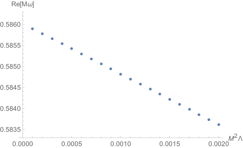
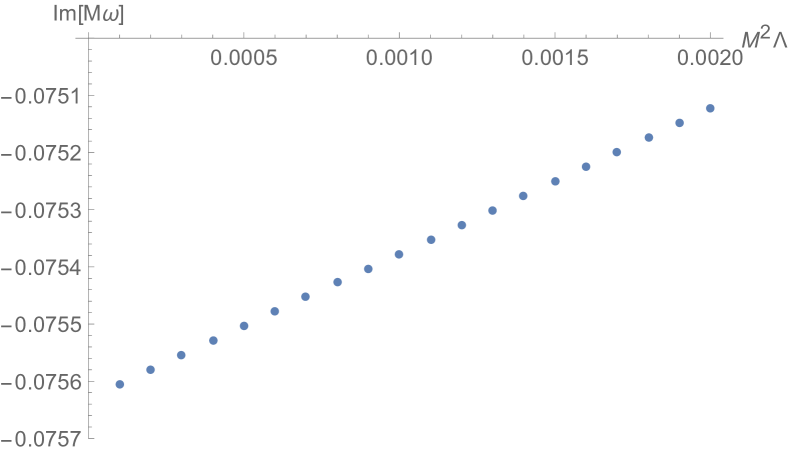
Figure 1: These panels show the real and imaginary parts of $M{}_{-2}\omega_{22}$ for almost asymptotically flat black holes at $a/M=4/5$. We can extrapolate them to the strictly flat case.

Another possible resolution has been proposed in fiziev2006 ; fiziev2010 . In this approach, a confluent Heun solution at $z=1$ is analytically continued to infinity that is an irregular singular point. It would be interesting to apply ‘HeunC’ to asymptotically flat rotating black holes along this line.

- (1) https://reference.wolfram.com/language/ref/HeunG.html.
- (2) A. Ronveaux, Heun’s Differential Equations, Oxford University Press, Oxford, New York, October 1995.
- (3) G. Kristensson, Second Order Differential Equations: Special Functions and Their Classification, Springer Science & Business Media, August 2010.
- (4) DLMF: 31 Heun Functions, https://dlmf.nist.gov/31.
- (5) https://www.maplesoft.com/support/help/Maple/view.aspx?path=HeunG.
- (6) P. P. Fiziev, Exact solutions of Regge–Wheeler equation and quasi-normal modes of compact objects, Class. Quantum Grav. 23 (2006) 2447–2468.
- (7) O. V. Motygin, On numerical evaluation of the Heun functions, May 2015, https://github.com/motygin/Heun_functions.
- (8) T. Birkandan and M. Hortaçsu, Quantum field theory applications of heun type functions, Rept. Math. Phys. 79 (2017) 81–87.
- (9) M. Hortaçsu, Heun Functions and Some of Their Applications in Physics, Adv. High Energy Phys. 2018 (2018) 8621573.
- (10) S. A. Teukolsky, Rotating Black Holes: Separable Wave Equations for Gravitational and Electromagnetic Perturbations, Phys. Rev. Lett. 29 (1972) 1114–1118.
- (11) H. Suzuki, E. Takasugi and H. Umetsu, Perturbations of Kerr-de Sitter Black Holes and Heun’s Equations, Prog. Theor. Phys. 100 (1998) 491–505.
- (12) R. Maier, The 192 solutions of the Heun equation, Math. Comp. 76 (2007) 811–843.
- (13) P. P. Fiziev, Classes of exact solutions to the Teukolsky master equation, Class. Quantum Grav. 27 (2010) 135001.
- (14) U. Khanal, Rotating black hole in asymptotic de Sitter space: Perturbation of the space-time with spin fields, Phys. Rev. D 28 (1983) 1291–1297.
- (15) C. M. Chambers and I. G. Moss, Stability of the Cauchy horizon in Kerr–de Sitter spacetimes, Class. Quantum Grav. 11 (1994) 1035–1054.
- (16) G. Aminov, A. Grassi and Y. Hatsuda, Black Hole Quasinormal Modes and Seiberg-Witten Theory, arXiv:2006.06111 [hep-th].
- (17) M. Giammatteo and I. G. Moss, Gravitational quasinormal modes for Kerr anti-de Sitter black holes, Class. Quantum Grav. 22 (2005) 1803–1824.
- (18) E. W. Leaver, An analytic representation for the quasi-normal modes of Kerr black holes, Proc. R. Soc. Lond. A. 402 (1985) 285–298.
- (19) A. Jansen, Overdamped modes in Schwarzschild-de Sitter and a Mathematica package for the numerical computation of quasinormal modes, Eur. Phys. J. Plus 132 (2017) 546.
- (20) Y. Hatsuda, Quasinormal modes of black holes and Borel summation, Phys. Rev. D 101 (2020) 024008.
- (21) A. Zhidenko, Quasi-normal modes of Schwarzschild–de Sitter black holes, Class. Quantum Grav. 21 (2003) 273–280.
- (22) S. Yoshida, N. Uchikata and T. Futamase, Quasinormal modes of Kerr–de Sitter black holes, Phys. Rev. D 81 (2010) 044005.
- (23) F. Novaes, C. I. S. Marinho, M. Lencsés and M. Casals, Kerr-de Sitter quasinormal modes via accessory parameter expansion, J. High Energ. Phys. 2019 (2019) 33.
- (24) C. M. Bender and S. A. Orszag, Advanced mathematical methods for scientists and engineers, McGraw-Hill, 1978.
- (25) https://pages.jh.edu/~eberti2/ringdown/.