Federated Accelerated Stochastic Gradient Descent

Abstract

We propose Federated Accelerated Stochastic Gradient Descent (FedAc), a principled acceleration of Federated Averaging (FedAvg, also known as Local SGD) for distributed optimization. FedAc is the first provable acceleration of FedAvg that improves convergence speed and communication efficiency on various types of convex functions. For example, for strongly convex and smooth functions, when using $M$ workers, the previous state-of-the-art FedAvg analysis can achieve a linear speedup in $M$ if given $\operatorname{\tilde{\mathcal{O}}}(M)$ rounds of synchronization, whereas FedAc only requires $\operatorname{\tilde{\mathcal{O}}}(M^{\frac{1}{3}})$ rounds. Moreover, we prove stronger guarantees for FedAc when the objectives are third-order smooth. Our technique is based on a potential-based perturbed iterate analysis, a novel stability analysis of generalized accelerated SGD, and a strategic tradeoff between acceleration and stability.

1 Introduction

Leveraging distributed computing resources and decentralized data is crucial, if not necessary, for large-scale machine learning applications. Communication is usually the major bottleneck for parallelization in both data-center settings and cross-device federated settings (Kairouz et al., 2019).

We study the distributed stochastic optimization $\min_{w\in\mathbb{R}^{d}}F(w):=\operatorname{\mathbb{E}}_{\xi\sim\mathcal{D}}f(w;\xi)$ where $F$ is convex. We assume there are $M$ parallel workers and each worker can access $F$ at $w$ via oracle $\nabla f(w;\xi)$ for independent sample $\xi$ drawn from distribution $\mathcal{D}$. We assume synchronization (communication) among workers is allowed but limited to $R$ rounds. We denote $T$ as the parallel runtime.

One of the most common and well-studied algorithms for this setting is Federated Averaging (FedAvg) (McMahan et al., 2017), also known as Local SGD or Parallel SGD (Mangasarian, 1995; Zinkevich et al., 2010; Coppola, 2014; Zhou and Cong, 2018) in the literature. In FedAvg, each worker runs a local thread of SGD (Robbins and Monro, 1951), and periodically synchronizes with other workers by collecting the averages and broadcast to all workers. The analysis of FedAvg (Stich, 2019a; Stich and Karimireddy, 2019; Khaled et al., 2020; Woodworth et al., 2020) usually follows the perturbed iterate analysis framework (Mania et al., 2017) where the performance of FedAvg is compared with the idealized version with infinite synchronization. The key idea is to control the stability of SGD so that the local iterates held by parallel workers do not differ much, even with infrequent synchronization.

We study the acceleration of FedAvg and investigate whether it is possible to improve convergence speed and communication efficiency. The main challenge for introducing acceleration lies in the disaccord of acceleration and stability. Stability is essential for analyzing distributed algorithms such as FedAvg, whereas momentum applied for acceleration may amplify the instability of the algorithm. Indeed, we show that standard Nesterov accelerated gradient descent algorithm (Nesterov, 2018) may not be initial-value stable even for smooth and strongly convex functions, in the sense that the initial infinitesimal difference may grow exponentially fast (see Theorem 4.2). This evidence necessitates a more scrutinized acceleration in distributed settings.

We propose a principled acceleration for FedAvg, namely Federated Accelerated Stochastic Gradient Descent (FedAc), which provably improves convergence rate and communication efficiency. Our result extends the results of Woodworth et al. (2020) on Local-Ac-Sa for quadratic objectives to broader objectives. To the best of our knowledge, this is the first provable acceleration of FedAvg (and its variants) for general or strongly convex objectives. FedAc parallelizes a generalized version of Accelerated SGD (Ghadimi and Lan, 2012), while we carefully balance the acceleration-stability tradeoff to accommodate distributed settings. Under standard assumptions on smoothness, bounded variance, and strong convexity (see Assumption 1 for details), FedAc converges at rate $\operatorname{\tilde{\mathcal{O}}}(\frac{1}{MT}+\frac{1}{TR^{3}})$. The bound will be dominated by $\operatorname{\tilde{\mathcal{O}}}(\frac{1}{MT})$ for $R$ as low as $\operatorname{\tilde{\mathcal{O}}}(M^{\frac{1}{3}})$, which implies the synchronization $R$ required for linear speedup in $M$ is $\operatorname{\tilde{\mathcal{O}}}(M^{\frac{1}{3}})$. In comparison, the state-of-the-art FedAvg analysis Khaled et al. (2020) showed that FedAvg converges at rate $\operatorname{\tilde{\mathcal{O}}}(\frac{1}{MT}+\frac{1}{TR})$, which requires $\operatorname{\tilde{\mathcal{O}}}(M)$ synchronization for linear speedup. For general convex objective, FedAc converges at rate $\operatorname{\tilde{\mathcal{O}}}(\frac{1}{\sqrt{MT}}+\frac{1}{T^{\frac{1}{3}}R^{\frac{2}{3}}})$, which outperforms both state-of-the-art FedAvg $\operatorname{\tilde{\mathcal{O}}}(\frac{1}{\sqrt{MT}}+\frac{1}{T^{\frac{1}{3}}R^{\frac{1}{3}}})$ by Woodworth et al. and Minibatch-SGD baseline ${\Theta}(\frac{1}{\sqrt{MT}}+\frac{1}{R})$ (Dekel et al., 2012). We summarize communication bounds and convergence rates in Tables 1 and 2 (on the row marked A1).

Table 1: Summary of results on the synchronization rounds $R$ required for linear speedup in $M$. All bounds hide multiplicative $\operatorname{\mathrm{polylog}}$ factors and variables other than $M$ and $T$ for ease of presentation. Notation: $M$: number of workers; $T$: parallel runtime.

		Synchronization Required for Linear Speedup
Assumption	Algorithm	Strongly Convex	General Convex	Reference
Assumption 1	FedAvg	$T^{\frac{1}{2}}M^{\frac{1}{2}}$	–	(Stich, 2019a)
		$T^{\frac{1}{3}}M^{\frac{1}{3}}$	–	(Haddadpour et al., 2019b)
		$M$	$T^{\frac{1}{2}}M^{\frac{3}{2}}$	(Stich and Karimireddy, 2019)
		$M$	$T^{\frac{1}{2}}M^{\frac{3}{2}}$	(Khaled et al., 2020)
	FedAc	$\bm{M^{\frac{1}{3}}}$	$\min\{\bm{T^{\frac{1}{4}}M^{\frac{3}{4}}},\bm{T^{\frac{1}{3}}M^{\frac{2}{3}}}\}$	Theorems 3.1, E.1 and E.2
Assumption 2	FedAvg	$\max\{\bm{T^{-\frac{1}{2}}M^{\frac{1}{2}}},\bm{1}\}$	${T^{\frac{1}{2}}M^{\frac{3}{2}}}$	Theorems 3.4 and E.4
	FedAc	$\max\{\bm{T^{-\frac{1}{6}}M^{\frac{1}{6}}},\bm{1}\}$	$\max\{\bm{T^{\frac{1}{4}}M^{\frac{1}{4}}},\bm{T^{\frac{1}{6}}M^{\frac{1}{2}}}\}$	Theorems 3.3 and E.3

Our results suggest an intriguing synergy between acceleration and parallelization. In the single-worker sequential setting, the convergence is usually dominated by the term related to stochasticity, which is in general not possible to be accelerated (Nemirovski and Yudin, 1983). In distributed settings, the communication efficiency is dominated by the overhead caused by infrequent synchronization, which can be accelerated as we show in the convergence rates summary Table 2.

Table 2: Summary of results on convergence rates. All bounds omit multiplicative $\operatorname{\mathrm{polylog}}$ factors and additive exponential decaying term (for strongly convex objective) for ease of presentation. Notation: $D_{0}$: $\|w_{0}-w^{*}\|$; $M$: number of workers; $T$: parallel runtime; $R$: synchronization; $\mu$: strong convexity; $L$: smoothness; $Q$: 3^rd-order-smoothness (in Assumption 2).

Assumption	Algorithm	Convergence Rate $(\operatorname{\mathbb{E}}[F(\cdot)]-F^{*}\leq\cdots$)	Reference
A1($\mu>0$)	FedAvg	exp. decay $+\frac{\sigma^{2}}{\mu MT}+\frac{L\sigma^{2}}{\mu^{2}TR}$	(Woodworth et al., 2020)
	FedAc	exp. decay $+\frac{\sigma^{2}}{\mu MT}+\min\left\{\frac{L\sigma^{2}}{\mu^{2}TR^{2}},\frac{L^{2}\sigma^{2}}{\mu^{3}TR^{3}}\right\}$	Theorem 3.1
A2($\mu>0$)	FedAvg	exp. decay $+\frac{\sigma^{2}}{\mu MT}+\frac{Q^{2}\sigma^{4}}{\mu^{5}T^{2}R^{2}}$	Theorem 3.4
	FedAc	exp. decay $+\frac{\sigma^{2}}{\mu MT}+{\frac{Q^{2}\sigma^{4}}{\mu^{5}T^{2}R^{6}}}$	Theorem 3.3
A1($\mu=0$)	FedAvg	$\frac{LD_{0}^{2}}{T}+\frac{\sigma D_{0}}{\sqrt{MT}}+\frac{L^{\frac{1}{3}}\sigma^{\frac{2}{3}}D_{0}^{\frac{4}{3}}}{T^{\frac{1}{3}}R^{\frac{1}{3}}}$	(Woodworth et al., 2020)
	FedAc	$\frac{LD_{0}^{2}}{TR}+\frac{\sigma D_{0}}{\sqrt{MT}}+\min\left\{\frac{L^{\frac{1}{3}}\sigma^{\frac{2}{3}}D_{0}^{\frac{4}{3}}}{T^{\frac{1}{3}}R^{\frac{2}{3}}},\frac{L^{\frac{1}{2}}\sigma^{\frac{1}{2}}D_{0}^{\frac{3}{2}}}{T^{\frac{1}{4}}R^{\frac{3}{4}}}\right\}$	Theorems E.1 and E.2
A2($\mu=0$)	FedAvg	$\frac{LD_{0}^{2}}{T}+\frac{\sigma D_{0}}{\sqrt{MT}}+\frac{Q^{\frac{1}{3}}\sigma^{\frac{2}{3}}D_{0}^{\frac{5}{3}}}{T^{\frac{1}{3}}R^{\frac{1}{3}}}$	Theorem E.4
	FedAc	$\frac{LD_{0}^{2}}{TR}+\frac{\sigma D_{0}}{\sqrt{MT}}+\frac{L^{\frac{1}{3}}\sigma^{\frac{2}{3}}D_{0}^{\frac{4}{3}}}{M^{\frac{1}{3}}T^{\frac{1}{3}}R^{\frac{2}{3}}}+\frac{Q^{\frac{1}{3}}\sigma^{\frac{2}{3}}D_{0}^{\frac{5}{3}}}{T^{\frac{1}{3}}R}$	Theorem E.3

We establish stronger guarantees for FedAc when objectives are 3^rd-order-smooth, or “close to be quadratic” intuitively (see Assumption 2 for details). For strongly convex objectives, FedAc converges at rate $\operatorname{\tilde{\mathcal{O}}}(\frac{1}{MT}+\frac{1}{T^{2}R^{6}})$ (see Theorem 3.3). We also prove the convergence rates of FedAvg in this setting for comparison. We summarize our results in Tables 1 and 2 (on the row marked A2).

We empirically verify the efficiency of FedAc in Section 5. Numerical results suggest a considerable improvement of FedAc over all three baselines, namely FedAvg, (distributed) Minibatch-SGD, and (distributed) Accelerated Minibatch-SGD (Dekel et al., 2012; Cotter et al., 2011), especially in the regime of highly infrequent communication and abundant workers.

1.1 Related work

The analysis of FedAvg (a.k.a. Local SGD) is an active area of research. Early research on FedAvg mostly focused on the particular case of $R=1$, also known as “one-shot averaging”, where the iterates are only averaged once at the end of procedure (Mcdonald et al., 2009; Zinkevich et al., 2010; Zhang et al., 2013; Shamir and Srebro, 2014; Rosenblatt and Nadler, 2016). The first convergence result on FedAvg with general (more than one) synchronization for convex objectives was established by Stich (2019a) under the assumption of uniformly bounded gradients. Stich and Karimireddy (2019); Haddadpour et al. (2019b); Dieuleveut and Patel (2019); Khaled et al. (2020) relaxed this requirement and studied FedAvg under assumptions similar to our Assumption 1. These works also attained better rates than (Stich, 2019a) through an improved stability analysis of SGD. However, recent work (Woodworth et al., 2020) showed that all the above bounds on FedAvg are strictly dominated by minibatch SGD (Dekel et al., 2012) baseline. Woodworth et al. (2020) provided the first bound for FedAvg that can improve over minibatch SGD for certain cases. This is to our knowledge the state-of-the-art bound for FedAvg and its variants. Our FedAc uniformly dominates this bound on FedAvg.

The specialty of quadratic objectives for better communication efficiency has been studied in an array of contexts (Zhang et al., 2015; Jain et al., 2018). Woodworth et al. (2020) studied an acceleration of FedAvg but was limited to quadratic objectives. More generally, Dieuleveut and Patel (2019) studied the convergence of FedAvg under bounded 3^rd-derivative, but the bounds are still dominated by minibatch SGD baseline (Woodworth et al., 2020). Recent work by Godichon-Baggioni and Saadane (2020) studied one-shot averaging under similar assumptions. Our analysis on FedAvg (Theorem 3.4) allows for general $R$ and reduces to a comparable bound if $R=1$, which is further improved by our analysis on FedAc (Theorem 3.3).

FedAvg has also been studied in other more general settings. A series of recent papers (e.g., (Zhou and Cong, 2018; Haddadpour et al., 2019a; Wang and Joshi, 2019; Yu and Jin, 2019; Yu et al., 2019a, b)) studied the convergence of FedAvg for non-convex objectives. We conjecture that FedAc can be generalized to non-convex objectives to attain better efficiency by combining our result with recent non-convex acceleration algorithms (e.g., (Carmon et al., 2018)). Numerous recent papers (Khaled et al., 2020; Li et al., 2020b; Haddadpour and Mahdavi, 2019; Koloskova et al., 2020) studied FedAvg in heterogeneous settings, where each worker has access to stochastic gradient oracles from different distributions. Other variants of FedAvg have been proposed in the face of heterogeneity (Pathak and Wainwright, 2020; Li et al., 2020a; Karimireddy et al., 2020; Wang et al., 2020). We defer the analysis of FedAc for heterogeneous settings for future work. Other techniques, such as quantization, can also reduce communication cost (Alistarh et al., 2017; Wen et al., 2017; Stich et al., 2018; Basu et al., 2019; Mishchenko et al., 2019; Reisizadeh et al., 2020). We refer readers to (Kairouz et al., 2019) for a more comprehensive survey of the recent development of algorithms in Federated Learning.

Stability is one of the major topics in machine learning and has been studied for a variety of purposes (Yu and Kumbier, 2020). For example, Bousquet and Elisseeff (2002); Hardt et al. (2016) showed that algorithmic stability can be used to establish generalization bounds. Chen et al. (2018) provided the stability bound of standard Accelerated Gradient Descent (AGD) for quadratic objectives. To the best of our knowledge, there is no existing (positive or negative) result on the stability of AGD for general convex or strongly convex objectives. This work provides the first (negative) result on the stability of standard deterministic AGD, which suggests that standard AGD may not be initial-value stable even for strongly convex and smooth objectives (Theorem 4.2). This result may be of broader interest. The tradeoff technique of FedAc also provides a possible remedy to mitigate the instability issue, which may be applied to derive better generalization bounds for momentum-based methods.

The stochastic optimization problem $\min_{w\in\mathbb{R}^{d}}F(w):=\operatorname{\mathbb{E}}_{\xi\sim\mathcal{D}}f(w;\xi)$ we consider in this paper is commonly referred to as the stochastic approximation (SA) problem in the literature (Kushner et al., 2003). Another related question is the sample average approximation (SAA), also known as empirical risk minimization (ERM) problem (Vapnik, 1998). The ERM problem is defined as $\min_{w\in\mathbb{R}^{d}}F(w):=\frac{1}{N}\sum_{i=1}^{N}f(w;\xi^{(i)})$, where the sum of a fixed finite set of objectives is to be optimized. For strongly-convex ERM, it is possible to leverage variance reduction techniques (Johnson and Zhang, 2013) to attain linear convergence. For example, the Distributed Accelerated SVRG (DA-SVRG) (Lee et al., 2017) can attain expected $\varepsilon$-optimality within $\tilde{\mathcal{O}}(\frac{N}{M}\log(1/\varepsilon))$ parallel runtime and $\tilde{\mathcal{O}}(\log(1/\varepsilon))$ rounds of communication. If we were to apply FedAc for ERM, it can attain expected $\varepsilon$-optimality with $\tilde{\mathcal{O}}(\frac{1}{M\varepsilon})$ parallel runtime and $\tilde{\mathcal{O}}(M^{\frac{1}{3}})$ rounds of communication (assuming Assumption 1 is satisfied). Therefore one can obtain low accuracy solution with FedAc in a short parallel runtime, whereas DA-SVRG may be preferred if high accuracy is required and $N$ is relatively small. It is worth mentioning that FedAc is not designed or proved for the distributed ERM setting, and we include this rough comparison for completeness. We conjecture that FedAc can be incorporated with appropriate variance reduction techniques to attain better performance in distributed ERM setting.

2 Preliminaries

2.1 Assumptions

We conduct our analysis on FedAc in two settings with two sets of assumptions. The following Assumption 1 consists of a set of standard assumptions: convexity, smoothness and bounded variance. Comparable assumptions are assumed in existing studies on FedAvg (Haddadpour et al., 2019b; Stich and Karimireddy, 2019; Khaled et al., 2020; Woodworth et al., 2020).

Assumption 1 ($\mu$-strong convexity, $L$-smoothness and $\sigma^{2}$-uniformly bounded gradient variance).

1. $F$ is $\mu$-strongly convex, i.e., $F(u)\geq F(w)+\langle\nabla F(w),u-w\rangle+\frac{1}{2}\mu\|u-w\|^{2}$ for any $u,w\in\mathbb{R}^{d}$. In addition, assume $F$ attains a finite optimum $w^{*}\in\mathbb{R}^{d}$. (We will study both the strongly convex case $(\mu>0)$ and the general convex case $(\mu=0)$, which will be clarified in the context.)

2. $F$ is $L$-smooth, i.e., $F(u)\leq F(w)+\langle\nabla F(w),u-w\rangle+\frac{1}{2}L\|u-w\|^{2}$ for any $u,w\in\mathbb{R}^{d}$.

3. $\nabla f(w;\xi)$ has $\sigma^{2}$-bounded variance, i.e., $\sup_{w\in\mathbb{R}^{d}}\operatorname{\mathbb{E}}_{\xi\in\mathcal{D}}\|\nabla f(w;\xi)-\nabla F(w)\|^{2}\leq\sigma^{2}$.

The following Assumption 2 consists of an additional set of assumptions: 3^rd order smoothness and bounded $4\textsuperscript{th}$ central moment. A similar version of Assumption 2 was studied in (Dieuleveut and Patel, 2019).

Assumption 2.

In addition to Assumption 1, assume that

1. $F$ is $Q$-3^rd-order-smooth, i.e., $F(u)\leq F(w)+\langle\nabla F(w),u-w\rangle+\frac{1}{2}\langle\nabla^{2}F(w)(u-w),(u-w)\rangle+\frac{1}{6}Q\|u-w\|^{3}$ for any $u,w\in\mathbb{R}^{d}$.

2. $\nabla f(w;\xi)$ has $\sigma^{4}$-bounded 4^th central moment, i.e, $\sup_{w\in\mathbb{R}^{d}}\operatorname{\mathbb{E}}_{\xi\in\mathcal{D}}\|\nabla f(w;\xi)-\nabla F(w)\|^{4}\leq\sigma^{4}$.

2.2 Notations

We use $\|\cdot\|$ to denote the operator norm of a matrix or the $\ell_{2}$-norm of a vector, $[n]$ to denote the set $\{1,2,\ldots,n\}$. Let $w^{*}$ be the optimum of $F$ and denote $F^{*}:=F(w^{*})$. Let $D_{0}:=\|w_{0}-w^{*}\|$. be the Euclidean distance of the initial guess $w_{0}$ and the optimum $w^{*}$. For both FedAc and FedAvg, we use $M$ to denote the number of parallel workers, $R$ to denote synchronization rounds, $K$ to denote the synchronization interval (i.e., the number of local steps per synchronization round), and $T=KR$ to denote the parallel runtime. We use the subscript to denote timestep, italicized superscript to denote the index of worker and unitalicized superscript “md” or “ag” to denote modifier of iterates in FedAc (see definition in Algorithm 1). We use overline to denote averaging over all workers, e.g., $\overline{w_{t}^{\mathrm{ag}}}:=\frac{1}{M}\sum_{m=1}^{M}w_{t}^{\mathrm{ag},m}$. We use $\operatorname{\tilde{\mathcal{O}}},\tilde{\Theta}$ to hide multiplicative $\operatorname{\mathrm{polylog}}$ factors, which will be clarified in the formal context.

3 Main results

3.1 Main algorithm: Federated Accelerated Stochastic Gradient Descent (FedAc)

We formally introduce our algorithm FedAc in Algorithm 1. FedAc parallelizes a generalized version of Accelerated SGD by Ghadimi and Lan (2012). In FedAc, each worker $m\in[M]$ maintains three intertwined sequences $\{w_{t}^{m},w_{t}^{\mathrm{ag},m},w_{t}^{\mathrm{md},m}\}$ at each step $t$. Here $w_{t}^{\mathrm{ag},m}$ aggregates the past iterates, $w_{t}^{\mathrm{md},m}$ is the auxiliary sequence of “middle points” on which the gradients are queried, and $w_{t}^{m}$ is the main sequence of iterates. At each step, candidate next iterates $v_{t+1}^{\mathrm{ag},m}$ and $v_{t+1}^{m}$ are computed. If this is a local (unsynchronized) step, they will be assigned to the next iterates $w_{t+1}^{\mathrm{ag},m}$ and $w_{t+1}^{\mathrm{ag},m}$. Otherwise, they will be collected, averaged, and broadcast to all the workers.

Algorithm 1 Federated Accelerated Stochastic Gradient Descent (FedAc)

1:procedure FedAc($\alpha,\beta,\eta,\gamma$) $\triangleright$ See Eqs. 3.1 and 3.2 for hyperparameter choices

2:     Initialize $w_{0}^{\mathrm{ag},m}=w_{0}^{m}=w_{0}$ for all $m\in[M]$

3:     for $t=0,\ldots,T-1$ do

4:         for every worker $m\in[M]$ in parallel do

5:              $w_{t}^{\mathrm{md},m}\leftarrow\beta^{-1}w_{t}^{m}+(1-\beta^{-1})w_{t}^{\mathrm{ag},m}$ $\triangleright$ Compute $w_{t}^{\mathrm{md,m}}$ by coupling

6:              $g_{t}^{m}\leftarrow\nabla f(w_{t}^{\mathrm{md},m};\xi_{t}^{m})$ $\triangleright$ Query gradient at $w_{t}^{\mathrm{md},m}$

7:              $v_{t+1}^{\mathrm{ag},m}\leftarrow w_{t}^{\mathrm{md},m}-\eta\cdot g_{t}^{m}$ $\triangleright$ Compute next iterate candidate $v_{t+1}^{\mathrm{ag},m}$

8:              $v_{t+1}^{m}\leftarrow(1-\alpha^{-1})w_{t}^{m}+\alpha^{-1}w_{t}^{\mathrm{md},m}-\gamma\cdot g_{t}^{m}$ $\triangleright$ Compute next iterate candidate $v_{t+1}^{m}$

9:              if  sync (i.e., $t~{}\textup{mod}~{}K=-1$) then

10:                  $w_{t+1}^{m}\leftarrow\frac{1}{M}\sum_{m^{\prime}=1}^{M}v_{t+1}^{m^{\prime}}$;  $w_{t+1}^{\mathrm{ag},m}\leftarrow\frac{1}{M}\sum_{m^{\prime}=1}^{M}v_{t+1}^{\mathrm{ag},m^{\prime}}$ $\triangleright$ Average & broadcast

11:              else

12:                  $w_{t+1}^{m}\leftarrow v_{t+1}^{m}$;  $w_{t+1}^{\mathrm{ag},m}\leftarrow v_{t+1}^{\mathrm{ag},m}$ $\triangleright$ Candidates assigned to be the next iterates                             

Hyperparameter choice.

We note that the particular version of Accelerated SGD in FedAc is more flexible than the most standard Nesterov version (Nesterov, 2018), as it has four hyperparameters instead of two. Our analysis suggests that this flexibility seems crucial for principled acceleration in the distributed setting to allow for acceleration-stability trade-off.

However, we note that our theoretical analysis gives a very concrete choice of hyperparameter $\alpha,\beta$, and $\gamma$ in terms of $\eta$. For $\mu$-strongly-convex objectives, we introduce the following two sets of hyperparameter choices, which are referred to as FedAc-I and FedAc-II, respectively. As we will see in the Section 3.2.1, under Assumption 1, FedAc-I has a better dependency on condition number $\nicefrac{{L}}{{\mu}}$, whereas FedAc-II has better communication efficiency.

$$\text{{FedAc-I}}:\quad \eta\in\left(0,\frac{1}{L}\right],\quad \gamma=\max\left\{\sqrt{\frac{\eta}{\mu K}},\eta\right\},\quad \alpha=\frac{1}{\gamma\mu},\quad \beta=\alpha+1;\ignorespaces\ignorespaces\addcontentsline{lla}{section}{\numberline{\string\crtrefnumber{fedaci}}{f}edaci}$$ (3.1)

$$\text{{FedAc-II}}:\quad \eta\in\left(0,\frac{1}{L}\right],\quad \gamma=\max\left\{\sqrt{\frac{\eta}{\mu K}},\eta\right\},\quad \alpha=\frac{3}{2\gamma\mu}-\frac{1}{2},\quad \beta=\frac{2\alpha^{2}-1}{\alpha-1}.\ignorespaces\ignorespaces\addcontentsline{lla}{section}{\numberline{\string\crtrefnumber{fedacii}}{f}edacii}$$ (3.2)

Therefore, practically, if the strong convexity estimate $\mu$ is given (which is often taken to be the $\ell_{2}$ regularization strength), the only hyperparameter to be tuned is $\eta$, whose optimal value depends on the problem parameters.

3.2 Theorems on the convergence for strongly convex objectives

Now we present main theorems of FedAc for strongly convex objectives under Assumption 1 or 2.

3.2.1 Convergence of FedAc under Assumption 1

We first introduce the convergence theorem on FedAc under Assumption 1. FedAc-I and FedAc-II lead to slightly different convergence rates.

Theorem 3.1 (Convergence of FedAc).

Let $F$ be $\mu>0$-strongly convex, and assume Assumption 1.

1. (Full version see Theorem B.1) For $\eta=\min\{\frac{1}{L},\tilde{\Theta}(\frac{1}{\mu TR})\}$, FedAc-I yields

   $$\operatorname{\mathbb{E}}\left[F({\overline{w_{T}^{\mathrm{ag}}}})-F^{*}\right]\leq\exp\left(\min\left\{-\frac{\mu T}{L},-\sqrt{\frac{\mu TR}{L}}\right\}\right)LD_{0}^{2}+\operatorname{\tilde{\mathcal{O}}}\left(\frac{\sigma^{2}}{\mu MT}+\frac{L\sigma^{2}}{\mu^{2}TR^{2}}\right).\addcontentsline{lla}{section}{\numberline{\string\crtrefnumber{eq:fedac:a1:1}}{e}q:fedac:a1:1}$$ (3.3)

2. (Full version see Theorem C.13) For $\eta=\min\{\frac{1}{L},\tilde{\Theta}(\frac{1}{\mu TR})\}$, FedAc-II yields

   $$\operatorname{\mathbb{E}}\left[F({\overline{w_{T}^{\mathrm{ag}}}})-F^{*}\right]\leq\exp\left(\min\left\{-\frac{\mu T}{3L},-\sqrt{\frac{\mu TR}{9L}}\right\}\right)LD_{0}^{2}+\operatorname{\tilde{\mathcal{O}}}\left(\frac{\sigma^{2}}{\mu MT}+\frac{L^{2}\sigma^{2}}{\mu^{3}TR^{3}}\right).\addcontentsline{lla}{section}{\numberline{\string\crtrefnumber{eq:fedac:a1:2}}{e}q:fedac:a1:2}$$ (3.4)

In comparison, the state-of-the-art FedAvg analysis (Khaled et al., 2020; Woodworth et al., 2020) reveals the following result.

Proposition 3.2 (Convergence of FedAvg under Assumption 1, adapted from Woodworth et al.).

In the settings of Theorem 3.1, for $\eta=\min\{\frac{1}{L},\tilde{\Theta}(\frac{1}{\mu T})\}$, for appropriate non-negative $\{\rho_{t}\}_{t=0}^{T-1}$ with $\sum_{t=0}^{T-1}\rho_{t}=1$, FedAvg yields

$$\operatorname{\mathbb{E}}\left[F\left(\sum_{t=0}^{T-1}\rho_{t}\overline{w_{t}}\right)-F^{*}\right]\leq\exp\left(-\frac{\mu T}{L}\right)LD_{0}^{2}+\operatorname{\tilde{\mathcal{O}}}\left(\frac{\sigma^{2}}{\mu MT}+\frac{L\sigma^{2}}{\mu^{2}TR}\right).\addcontentsline{lla}{section}{\numberline{\string\crtrefnumber{eq:fedavg:main}}{e}q:fedavg:main}$$ (3.5)

Remark.

The bound for FedAc-I (3.3) asymptotically universally outperforms FedAvg (3.5). The first term in (3.3) cooresponds to the deterministic convergence, which is better than the one for FedAvg. The second term corresponds to the stochasticity of the problem which is not improvable. The third term corresponds to the overhead of infrequent communication, which is also better than FedAvg due to acceleration. On the other hand, FedAc-II has better communication efficiency since the third term of (3.4) decays at rate $R^{-3}$.

3.2.2 Convergence of FedAc under Assumption 2 — faster when close to be quadratic

We establish stronger guarantees for FedAc-II (3.2) under Assumption 2.

Theorem 3.3 (Simplified version of Theorem C.1).

Let $F$ be $\mu>0$-strongly convex, and assume Assumption 2, then for $R\geq\sqrt{\frac{L}{\mu}}$, for $\eta=\min\{\frac{1}{L},\tilde{\Theta}(\frac{1}{\mu TR})\}$, FedAc-II yields

$$\operatorname{\mathbb{E}}\left[F({\overline{w_{T}^{\mathrm{ag}}}})-F^{*}\right]\leq\exp\left(\min\left\{-\frac{\mu T}{3L},-\sqrt{\frac{\mu TR}{9L}}\right\}\right)2LD_{0}^{2}+\operatorname{\tilde{\mathcal{O}}}\left(\frac{\sigma^{2}}{\mu MT}+\frac{Q^{2}\sigma^{4}}{\mu^{5}T^{2}R^{6}}\right).\addcontentsline{lla}{section}{\numberline{\string\crtrefnumber{eq:fedacii:a2}}{e}q:fedacii:a2}$$ (3.6)

In comparison, we also establish and prove the convergence rate of FedAvg under Assumption 2.

Theorem 3.4 (Simplified version of Theorem D.1).

In the settings of Theorem 3.3, for $\eta=\min\left\{\frac{1}{4L},\tilde{\Theta}\left(\frac{1}{\mu T}\right)\right\}$, for appropriate non-negative $\{\rho_{t}\}_{t=0}^{T-1}$ with $\sum_{t=0}^{T-1}\rho_{t}=1$, FedAvg yields

$$\operatorname{\mathbb{E}}\left[F\left(\sum_{t=0}^{T-1}{\rho_{t}}\overline{w_{t}}\right)-F^{*}\right]\leq\exp\left(-\frac{\mu T}{8L}\right)4LD_{0}^{2}+\operatorname{\tilde{\mathcal{O}}}\left(\frac{\sigma^{2}}{\mu MT}+\frac{Q^{2}\sigma^{4}}{\mu^{5}T^{2}R^{2}}\right).\addcontentsline{lla}{section}{\numberline{\string\crtrefnumber{eq:fedavg:a2}}{e}q:fedavg:a2}$$ (3.7)

Remark.

Our results give a smooth interpolation of the results of (Woodworth et al., 2020) for quadratic objectives to broader function class — the third term regarding infrequent communication overhead will vanish when the objective is quadratic since $Q=0$. The bound of FedAc (3.6) outperforms the bound of FedAvg (3.7) as long as $R\geq\sqrt{L/\mu}$ holds. Particularly in the case of $T\geq M$, our analysis suggests that only $\operatorname{\tilde{\mathcal{O}}}(1)$ synchronization are required for linear speedup in $M$. We summarize our results on synchronization bounds and convergence rate in Tables 1 and 2, respectively.

3.3 Convergence for general convex objectives

We also study the convergence of FedAc for general convex objectives ($\mu=0$). The idea is to apply FedAc to $\ell_{2}$-augmented objective $\tilde{F}_{\lambda}(w):=F(w)+\frac{\lambda}{2}\|w-w_{0}\|^{2}$ as a $\lambda$-strongly-convex and $(L+\lambda)$-smooth objective for appropriate $\lambda$, which is similar to the technique of (Woodworth et al., 2020). This augmented technique allows us to reuse most of the analysis for strongly-convex objectives. We conjecture that it is possible to construct direct versions of FedAc for general convex objectives that attain the same rates, which we defer for the future work. We summarize the synchronization bounds in Table 1 and the convergence rates in Table 2. We defer the statement of formal theorems to Section E in Appendix.

4 Proof sketch

In this section we sketch the proof for two of our main results, namely Theorem 3.1(a) and 3.3. We focus on the proof of Theorem 3.1(a) to outline our proof framework, and then illustrate the difference in the proof of Theorem 3.3.

4.1 Proof sketch of Theorem 3.1(a): FedAc-I under Assumption 1

Our proof framework consists of the following four steps.

Step 1: potential-based perturbed iterate analysis.

The first step is to study the difference between FedAc and its fully synchronized idealization, namely the case of $K=1$ (recall $K$ denotes the number of local steps). To this end, we extend the perturbed iterate analysis (Mania et al., 2017) to potential-based setting to analyze accelerated convergence. For FedAc-I, we study the decentralized potential $\Psi_{t}:=\frac{1}{M}\sum_{m=1}^{M}F({w_{t}^{\mathrm{ag},m}})-F^{*}+\frac{1}{2}\mu\|\overline{w_{t}}-w^{*}\|^{2}$ and establish the following lemma. $\Psi_{t}$ is adapted from the common potential for acceleration analysis (Bansal and Gupta, 2019).

Lemma 4.1 (Simplified version of Lemma B.2, Potential-based perturbed iterate analysis for FedAc-I).

In the same settings of Theorem 3.1(a), the following inequality holds

$$\operatorname{\mathbb{E}}\left[\Psi_{T}\right] \leq\exp\left(-\gamma\mu T\right)\Psi_{0}+\frac{\eta^{2}L\sigma^{2}}{2\gamma\mu}+\frac{\gamma\sigma^{2}}{2M} K=1$$ (Convergence rate in the case of )

$$+\underbrace{L\cdot\max_{0\leq t<T}\operatorname{\mathbb{E}}\left[\frac{1}{M}\sum_{m=1}^{M}\left\|\overline{w_{t}^{\mathrm{md}}}-w_{t}^{\mathrm{md},m}\right\|\left\|\frac{1}{1+\gamma\mu}(\overline{w_{t}}-w_{t}^{m})+\frac{\gamma\mu}{1+\gamma\mu}(\overline{w_{t}^{\mathrm{ag}}}-w_{t}^{\mathrm{ag},m})\right\|\right]}_{\text{Discrepancy overhead}}.\addcontentsline{lla}{section}{\numberline{\string\crtrefnumber{eq:fedaci:conv:sketch}}{e}q:fedaci:conv:sketch}$$ (4.1)

We refer to the last term of (4.1) as “discrepancy overhead” since it characterizes the dissimilarities among workers due to infrequent synchronization. The proof of Lemma 4.1 is deferred to Section B.2.

Step 2: bounding discrepancy overhead.

The second step is to bound the discrepancy overhead in (4.1) via stability analysis. Before we look into FedAc, let us first review the intuition for FedAvg. There are two forces governing the growth of discrepancy of FedAvg, namely the (negative) gradient and stochasticity. Thanks to the convexity, the gradient only makes the discrepancy lower. The stochasticity incurs $\mathcal{O}(\eta^{2}\sigma^{2})$ variance per step, so the discrepancy $\operatorname{\mathbb{E}}[\frac{1}{M}\sum_{m=1}^{M}\|\overline{w_{t}}-w_{t}^{m}\|^{2}]$ grows at rate $\mathcal{O}(\eta^{2}K\sigma^{2})$ linear in $K$. The detailed proof can be found in (Khaled et al., 2020; Woodworth et al., 2020).

For FedAc, the discrepancy analysis is subtler since acceleration and stability are at odds — the momentum may amplify the discrepancy accumulated from previous steps. Indeed, we establish the following Theorem 4.2, which shows that the standard deterministic Accelerated GD (Agd) may not be initial-value stable even for strongly convex and smooth objectives, in the sense that initial infinitesimal difference may grow exponentially fast. We defer the formal setup and the proof of Theorem 4.2 to Section F in Appendix.

Theorem 4.2 (Initial-value instability of deterministic standard Agd).

For any $L,\mu>0$ such that $\nicefrac{{L}}{{\mu}}\geq 25$, and for any $K\geq 1$, there exists a 1D objective $F$ that is $L$-smooth and $\mu$-strongly-convex, and an $\varepsilon_{0}>0$, such that for any positive $\varepsilon<\varepsilon_{0}$, there exists initialization $w_{0},u_{0},w_{0}^{\mathrm{ag}},u_{0}^{\mathrm{ag}}$ such that $|w_{0}-u_{0}|\leq\varepsilon$, $|w_{0}^{\mathrm{ag}}-u_{0}^{\mathrm{ag}}|\leq\varepsilon$, but the trajectories $\{w_{t}^{\mathrm{ag}},w_{t}^{\mathrm{md}},w_{t}\}_{t=0}^{3K}$, $\{u_{t}^{\mathrm{ag}},u_{t}^{\mathrm{md}},u_{t}\}_{t=0}^{3K}$ generated by applying deterministic Agd with initialization $(w_{0},w_{0}^{\mathrm{ag}})$ and $(u_{0},u_{0}^{\mathrm{ag}})$ satisfies

$$|w_{3K}-u_{3K}|\geq\frac{1}{2}\varepsilon(1.02)^{K},\qquad|w^{\mathrm{ag}}_{3K}-u^{\mathrm{ag}}_{3K}|\geq\varepsilon(1.02)^{K}.$$ (4.2)

Remark.

It is worth mentioning that the instability theorem does not contradicts the convergence of Agd (Nesterov, 2018). The convergence of Agd suggests that $w_{t}^{\mathrm{ag}}$, $w_{t}$, $u_{t}^{\mathrm{ag}}$, and $u_{t}$ will all converge to the same point $w^{*}$ as $t\to\infty$, which implies $\lim_{t\to\infty}\|w_{t}^{\mathrm{ag}}-u_{t}^{\mathrm{ag}}\|=\|w_{t}-u_{t}\|=0$. However, the convergence theorem does not imply the stability with respect to the initialization — it does not exclude the possibility that the difference between two instances (possibly with very close initialization) first expand and only shrink until they both approach $w^{*}$. Our Theorem 4.2 suggests this possibility: for any finite steps, no matter how small the (positive) initial difference is, it is possible that the difference will grow exponentially fast. This is fundamentally different from the Gradient Descent (for convex objectives), for which the difference between two instances does not expand for standard choice of learning rate $\eta=\frac{1}{L}$ (where $L$ is the smoothness).

Fortunately, we can show that the discrepancy can grow at a slower exponential rate via less aggressive acceleration, see Lemma 4.3. As we will discuss shortly, we adjust $\gamma$ according to $K$ to restrain the growth of discrepancy within the linear regime. The proof of Lemma 4.3 is deferred to Section B.3.

Lemma 4.3 (Simplified version of Lemma B.3, Discrepancy overhead bounds for FedAc-I).

In the same setting of Theorem 3.1(a), the following inequality holds

$$\text{``Discrepancy overhead'' in \lx@cref{creftype~refnum}{eq:fedaci:conv:sketch}}\leq\begin{cases}7\eta\gamma LK\sigma^{2}\left(1+\frac{2\gamma^{2}\mu}{\eta}\right)^{2K}&\text{if~{}}\gamma\in(\eta,\sqrt{\frac{\eta}{\mu}}],\\ 7\eta^{2}LK\sigma^{2}&\text{if~{}}\gamma=\eta.\end{cases}\addcontentsline{lla}{section}{\numberline{\string\crtrefnumber{eq:fedaci:stab:sketch}}{e}q:fedaci:stab:sketch}$$ (4.3)

Step 3: trading-off acceleration and discrepancy.

Combining Lemmas 4.1 and 4.3 gives

$$\addcontentsline{lla}{section}{\numberline{\string\crtrefnumber{fedaci:combine:sketch}}{f}edaci:combine:sketch}\operatorname{\mathbb{E}}\left[\Psi_{T}\right]\leq\underbrace{\exp\left(-\gamma\mu T\right)\Psi_{0}}_{\mathrm{(I)}}+\frac{\eta^{2}L\sigma^{2}}{2\gamma\mu}+\frac{\gamma\sigma^{2}}{2M}+\underbrace{\begin{cases}7\eta\gamma LK\sigma^{2}\left(1+\frac{2\gamma^{2}\mu}{\eta}\right)^{2K}&\text{if~{}}\gamma\in(\eta,\sqrt{\frac{\eta}{\mu}}],\\ 7\eta^{2}LK\sigma^{2}&\text{if~{}}\gamma=\eta.\end{cases}}_{\mathrm{(II)}}$$ (4.4)

The value of $\gamma\in[\eta,\sqrt{\eta/\mu}]$ controls the magnitude of acceleration in (I) and discrepancy growth in (II). The upper bound choice $\sqrt{\eta/\mu}$ gives full acceleration in (I) but makes (II) grow exponentially in $K$. On the other hand, the lower bound choice $\eta$ makes (II) linear in $K$ but loses all acceleration. We wish to attain as much acceleration in (I) as possible while keeping the discrepancy (II) grow moderately. Our balanced solution is to pick $\gamma=\max\{\sqrt{{\eta}/{(\mu K)}},\eta\}$. One can verify that the discrepancy grows (at most) linearly in $K$. Substituting this choice of $\gamma$ to Eq. 4.4 leads to

$$\operatorname{\mathbb{E}}\left[\Psi_{T}\right]\leq\underbrace{\exp\left(\min\left\{-\eta\mu T,-\frac{\eta^{\frac{1}{2}}\mu^{\frac{1}{2}}T}{K^{\frac{1}{2}}}\right\}\right)\Psi_{0}}_{\text{Monotonically decreasing }\varphi_{\downarrow}(\eta)}+\underbrace{\mathcal{O}\left(\frac{\eta^{\frac{1}{2}}\sigma^{2}}{\mu^{\frac{1}{2}}MK^{\frac{1}{2}}}+\frac{\eta\sigma^{2}}{M}+\frac{\eta^{\frac{3}{2}}LK^{\frac{1}{2}}\sigma^{2}}{\mu^{\frac{1}{2}}}+\eta^{2}LK\sigma^{2}\right)}_{\text{Monotonically increasing }\varphi_{\uparrow}(\eta)}.\addcontentsline{lla}{section}{\numberline{\string\crtrefnumber{eq:fedaci:eta:sketch}}{e}q:fedaci:eta:sketch}$$ (4.5)

Step 4: finding $\eta$ to optimize the RHS of Eq. 4.5.

It remains to show that (4.5) gives the desired bound with our choice of $\eta=\min\{\frac{1}{L},\tilde{\Theta}(\frac{K}{\mu T^{2}})\}$. The increasing $\varphi_{\uparrow}(\eta)$ in (4.5) is bounded by $\operatorname{\tilde{\mathcal{O}}}(\frac{\sigma^{2}}{\mu MT}+\frac{LK^{2}\sigma^{2}}{\mu^{2}T^{3}}).$ The decreasing term $\varphi_{\downarrow}(\eta)$ in (4.5) is bounded by $\varphi_{\downarrow}({\frac{1}{L}})+\varphi_{\downarrow}(\tilde{\Theta}(\frac{K}{\mu T^{2}}))$, where $\varphi_{\downarrow}({\frac{1}{L}})=\exp(\min\{-\frac{\mu T}{L},-\frac{\mu^{\frac{1}{2}}T}{L^{\frac{1}{2}}K^{\frac{1}{2}}}\})$, and $\varphi_{\downarrow}(\tilde{\Theta}(\frac{K}{\mu T^{2}}))\leq\exp\left(-\frac{\mu^{\frac{1}{2}}T}{K^{\frac{1}{2}}}\cdot\sqrt{\tilde{\Theta}\left(\frac{K}{\mu T^{2}}\right)}\right)$ can be controlled by the bound of $\varphi_{\uparrow}(\eta)$ provided $\tilde{\Theta}$ has appropriate $\operatorname{\mathrm{polylog}}$ factors. Plugging the bounds to (4.5) and replacing $K$ with $\nicefrac{{T}}{{R}}$ completes the proof of Theorem 3.1(a). We defer the details to Section B.

4.2 Proof sketch of Theorem 3.3: FedAc-II under Assumption 2

In this section, we outline the proof of Theorem 3.3 by explaining the differences with the proof in Section 4.1. The first difference is that for FedAc-II we study an alternative centralized potential $\Phi_{t}=F(\overline{w_{t}^{\mathrm{ag}}})-F^{*}+\frac{1}{6}\mu\|\overline{w_{t}}-w^{*}\|^{2}$, which leads to an alternative version of Lemma 4.1 as follows.

$$\operatorname{\mathbb{E}}[\Phi_{T}]\leq\exp\left(-\frac{\gamma\mu T}{3}\right)\Phi_{0}+\frac{3\eta^{2}L\sigma^{2}}{2\gamma\mu M}+\frac{\gamma\sigma^{2}}{2M}+\frac{3}{\mu}\max_{0\leq t<T}\operatorname{\mathbb{E}}\left\|\frac{1}{M}\sum_{m=1}^{M}\nabla F(w_{t}^{\mathrm{md},m})-\nabla F(\overline{w_{t}^{\mathrm{md}}})\right\|^{2}.\addcontentsline{lla}{section}{\numberline{\string\crtrefnumber{eq:fedacii:conv:sketch}}{e}q:fedacii:conv:sketch}$$ (4.6)

The second difference is that the particular discrepancy in (4.6) can be bounded via 3^rd-order smoothness $Q$ since (we omit “md” and $t$ to simplify the notations)

$$\left\|\frac{1}{M}\sum_{m=1}^{M}\nabla F(w^{m})-\nabla F(\overline{w})\right\|^{2}=\left\|\frac{1}{M}\sum_{m=1}^{M}\left(\nabla F(w^{m})-\nabla F(\overline{w})-\nabla^{2}F(\overline{w})(w^{m}-\overline{w_{t}})\right)\right\|^{2}$$ (4.7)

$$\leq \frac{1}{M}\sum_{m=1}^{M}\left\|\nabla F(w^{m})-\nabla F(\overline{w})-\nabla^{2}F(\overline{w})(w^{m}-\overline{w})\right\|^{2}\leq\frac{Q^{2}}{4M}\sum_{m=1}^{M}\left\|w^{m}-\overline{w}\right\|^{4}.$$ (4.8)

The proof then follows by analyzing the 4^th-order stability of FedAc. We defer the details to Section C.

5 Numerical experiments

In this section, we validate our theory and demonstrate the efficiency of FedAc via experiments. The performance of FedAc is tested against FedAvg (a.k.a., Local SGD), (distributed) Minibatch-SGD (Mb-Sgd) and Minibatch-Accelerated-SGD (Mb-Ac-Sgd) (Dekel et al., 2012; Cotter et al., 2011) on $\ell_{2}$-regularized logistic regression for UCI a9a dataset (Dua and Graff, 2017) from LibSVM (Chang and Lin, 2011). The regularization strength is set as $10^{-3}$. The hyperparameters $(\gamma,\alpha,\beta)$ of FedAc follows FedAc-I where strong-convexity $\mu$ is chosen as regularization strength $10^{-3}$. We test the settings of $M=2^{2},\ldots,2^{13}$ workers and $K=2^{0},\ldots,2^{8}$ synchronization interval. For all four algorithms, we tune the learning-rate $\eta$ only from the same set of levels within $[10^{-3},10]$. We choose $\eta$ based on the best suboptimality (regularized population loss). We claim that the best $\eta$ lies in the range $[10^{-3},10]$ for all algorithms under all settings. We defer the rest of setup details to Section A. In Fig. 1, we compare the algorithms by measuring the effect of linear speedup under variant $K$.

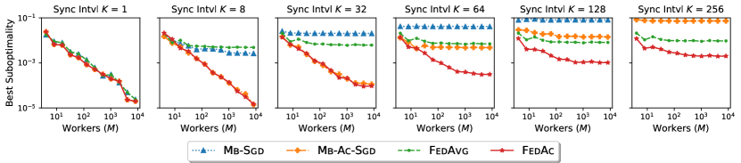
Figure 1: Observed linear speedup with respect to the number of workers $M$ under various synchronization intervals $K$. Our FedAc is tested against three baselines FedAvg, Mb-Sgd, and Mb-Ac-Sgd. While all four algorithms attain linear speedup for the fully synchronized ($K=1$) setting, FedAvg and Mb-Sgd lose linear speedup for $K$ as low as 8. Mb-Ac-Sgd is comparably better than the other two baselines but still deteriorates significantly for $K\geq 64$. FedAc is most robust to infrequent synchronization and outperforms the baselines by a margin for $K\geq 64$.

In the next experiments, we provide an empirical example to show that the direct parallelization of standard accelerated SGD may indeed suffer from instability. This complements our Theorem 4.2) on the initial-value instability of standard AGD. Recall that FedAc-I Eq. 3.1 and FedAc-II Eq. 3.2 adopt an acceleration-stability tradeoff technique that takes $\gamma=\max\{\sqrt{\frac{\eta}{\mu K}},\eta\}$. Formally, we denote the following direct acceleration of FedAc without such tradeoff as “vanilla FedAc”: $\eta\in(0,\frac{1}{L}],\gamma=\sqrt{\frac{\eta}{\mu}},\alpha=\frac{1}{\gamma\mu},\beta=\alpha+1.$ In Fig. 2, we compare the vanilla FedAc with the (stable) FedAc-I and the baseline Mb-Ac-Sgd.

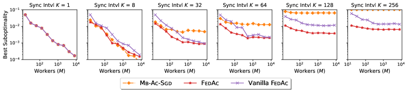
Figure 2: Vanilla FedAc versus (stable) FedAc-I and baseline Mb-Ac-Sgd on the observed linear speedup w.r.t. $M$ under various synchronization intervals $K$. Observet that Vanilla FedAc is indeed less robust to infrequent synchronization and thus worse than the FedAc-I. (dataset: a9a, $\lambda=10^{-4}$)

We include more experiments on various dataset, and more detailed analysis in Section A.

6 Conclusions

This work proposes FedAc, a principled acceleration of FedAvg, which provably improves convergence speed and communication efficiency. Our theory and experiments suggest that FedAc saves runtime and reduces communication overhead, especially in the setting of abundant workers and infrequent communication. We establish stronger guarantees when the objectives are third-order smooth. As a by-product, we also study the stability property of accelerated gradient descent, which may be of broader interest. We expect FedAc could be generalized to broader settings, e.g., non-convex objective and/or heterogenous workers.

The appendices are structured as follows. In Section A, we include additional experiments with description of setup details. In Sections B and C, we prove the complete version of Theorems 3.1 and 3.3 on the convergence of FedAc under Assumption 1 or 2. In Section D, we prove Theorem 3.4 on the convergence of FedAvg under Assumption 2. In Section E, we prove the convergence of FedAc (and FedAvg) for general convex objectives. In Section F, we prove Theorem 4.2 on the initial-value instability of standard accelerated gradient descent. We include some helper lemmas in Section G.

Appendix A Additional experiments and setup details

A.1 Additional setup details

Baselines.

FedAc is tested against three baselines, namely FedAvg (a.k.a., Local SGD), (distributed) Minibatch-SGD (Mb-Sgd), and (distributed) Minibatch-Accelerated-SGD (Mb-Ac-Sgd) (Dekel et al., 2012; Cotter et al., 2011). We fix the parallel runtime $T=4096$, and test variant levels of synchronization interval $K$ and parallel workers $M$. Mb-Sgd and Mb-Ac-Sgd baselines correspond to running SGD or accelerated SGD for $\nicefrac{{T}}{{K}}$ steps with batch size $MK$. The comparison is fair since all algorithms can be parallelized to $M$ workers with $\nicefrac{{T}}{{K}}$ rounds of communication where each worker queries $T$ gradients in total. We simulate the parallelization with a NumPy program on a local CPU cluster. We start from the same random initialization for all algorithms under all settings.

Datasets.

The algorithms are tested on $\ell_{2}$-regularized logistic regression on the following two binary classification datasets from LibSVM. The preprocessing information and the download links can be found at https://www.csie.ntu.edu.tw/~cjlin/libsvmtools/datasets/binary.html.

1. The “adult” a9a dataset with 123 features and 32,561 training samples from the UCI Machine Learning Repository (Dua and Graff, 2017).

2. The epsilon dataset with 2,000 features and 400,000 training samples from the PASCAL Challenge 2008 (Sonnenburg et al., 2008).

Evaluation.

For all algorithms and all settings, we evaluate the suboptimality (regularized population loss) every $512$ parallel timesteps (gradient queries). We compute the suboptimality by comparing with a pre-computed optimum $F^{*}$. We record the best suboptimality attained over the evaluations.

Hyperparameter choice.

For all four algorithms, we tune the “learning-rate” hyperparameter $\eta$ only and record the best suboptimality attained. For Mb-Ac-Sgd, the rest of hyperparameters are determined by the strong-convexity estimate $\mu$ which is taken to be the $\ell_{2}$-regularization strength $\lambda$. For FedAc, the default choice is FedAc-I Eq. 3.1, where the strong-convexity estimate $\mu$ is also taken to be the $\ell_{2}$-regularization strength $\lambda$.

A.2 Results on dataset a9a

We first test on the a9a dataset with $\ell_{2}$-regularization strength $10^{-3}$. We test the setting of $K=2^{0},\ldots,2^{8}$ and $M=2^{2},\ldots,2^{13}$. For all algorithms, we tune $\eta$ from the same sets: {0.001, 0.002, 0.005, 0.01, 0.02, 0.05, 0.1, 0.2, 0.5, 1, 2, 5, 10}. We claim that the best $\eta$ lies in $[0.001,10]$ for all algorithms for all settings. We plot the observed linear speedup figure in Fig. 1 in the main body. To better understand the dependency on synchronization intervals $K$, we plot the following Fig. 3. The results suggest that FedAc is more robust to infrequent synchronization and thus more communication-efficient. For example, when using 8192 workers, FedAc requries only 32 rounds of communication to attain $10^{-3}$ suboptimality, whereas Mb-Ac-Sgd, Mb-Sgd and FedAvg require 128, 1024, 4096 rounds, respectively.

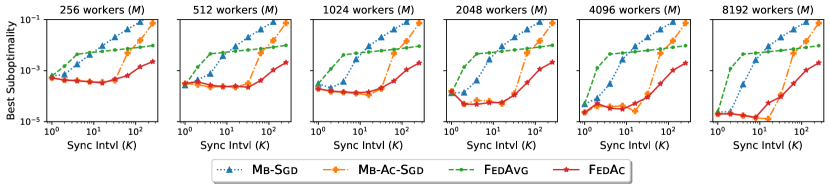
Figure 3: FedAc versus baselines on the dependency of synchronization interval $K$ under various workers $M$. For all tested $M$, FedAvg and Mb-Sgd start to deteriorate once $K$ passes $2$; Mb-Ac-Sgd is more robust to moderate $K$ than FedAvg and Mb-Sgd but sharply deteriorate once it passes a threshold at around $K=32$. This is because Mb-Ac-Sgd does not have enough gradient steps for convergence when the communication is too sparse. In comparison, FedAc is more robust to infrequent communication. Dataset: a9a, $\ell_{2}$-regularization strength: $10^{-3}$.

We repeat the experiments with an alternative choice of $\lambda=10^{-2}$. This problem is relatively “easier” in terms of optimization since the condition number $\nicefrac{{L}}{{\mu}}$ is lower. We test the same levels of $M$, $K$ and tune the $\eta$ from the same set as above. The results are shown in Figs. 4 and 5. The results are qualitatively similar to the $\lambda=10^{-3}$ case. For $K\leq 64$, the performance of FedAc and Mb-Ac-Sgd are similar, which both outperform the other two baselines FedAvg and Mb-Sgd. For $K\geq 128$, the Mb-Ac-Sgd drastically worsen because the gradient steps are too few, and FedAc outperforms the other baselines by a margin.

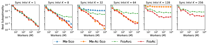
Figure 4: FedAc versus baselines on the observed linear speedup w.r.t $M$ under various synchronization interval $K$.   The results are qualitatively similar to Fig. 1. Dataset: a9a, $\ell_{2}$-regularization strength: $10^{-2}$.

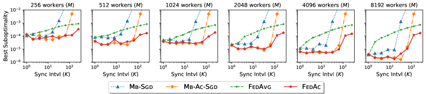
Figure 5: FedAc versus baselines on the dependency of synchronization interval $K$ under various workers $M$. The results are qualitatively similar to Fig. 3. Dataset: a9a, $\ell_{2}$-regularization strength: $10^{-2}$.

A.3 Results on dataset epsilon

In this section we repeat the experiments above on the larger epsilon dataset with $\ell_{2}$-regularization $\lambda$ taken to be $10^{-4}$. $\eta$ is tuned from $\{0.005,0.01,0.02,0.05,0.1,0.2,0.5,1,2,5,10,20,50\}$. The optimal $\eta$ lies in the corresponding range for all algorithm under all tested settings. The results are shown in Figs. 6 and 7. The results are qualitatively similar to the previous experiments on a9a dataset. FedAc is more communication-efficient than the baselines. For example, when using 2048 workers, FedAc requires only 64 rounds of communication (synchronization) to attain $10^{-4}$ suboptimality, whereas Mb-Ac-Sgd, Mb-Sgd and FedAvg require 256, 4096 and 4096 rounds of communication, respectively.

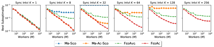
Figure 6: FedAc versus baselines on the observed linear speedup w.r.t $M$ under various synchronization interval $K$. The results are qualitatively similar to Fig. 1. Dataset: epsilon, $\ell_{2}$-regularization strength: $10^{-4}$.

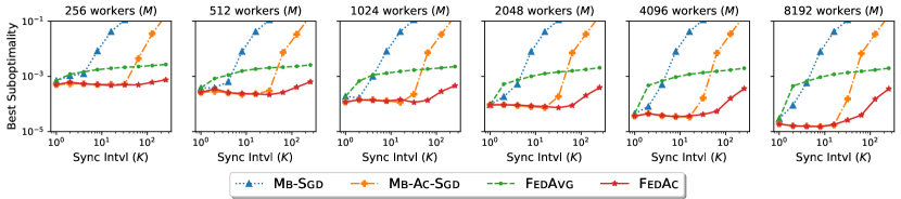
Figure 7: FedAc versus baselines on the dependency of synchronization interval $K$ under various workers $M$. The results are qualitatively similar to Fig. 3. Dataset: epsilon, $\ell_{2}$-regularization strength: $10^{-4}$.

Appendix B Analysis of FedAc-I under Assumption 1

In this section we study the convergence of FedAc-I. We provide a complete, non-asymptotic version of Theorem 3.1(a) on the convergence of FedAc-I under Assumption 1 and provide the detailed proof, which expands the proof sketch in Section 4.1. Recall that FedAc-I is defined as the FedAc (Algorithm 1) with the following hyperparameters choice

$$\eta\in\left(0,\frac{1}{L}\right],\quad\gamma=\max\left\{\sqrt{\frac{\eta}{\mu K}},\eta\right\},\quad\alpha=\frac{1}{\gamma\mu},\quad\beta=\alpha+1.$$ (FedAc-I)

We keep track of the convergence progress of FedAc-I via the following decentralized potential $\Psi_{t}$.

$$\Psi_{t}:=\frac{1}{M}\sum_{m=1}^{M}F({w_{t}^{\mathrm{ag},m}})-F^{*}+\frac{1}{2}\mu\|\overline{w_{t}}-w^{*}\|^{2}.\addcontentsline{lla}{section}{\numberline{\string\crtrefnumber{eq:fedaci:potential}}{e}q:fedaci:potential}$$ (B.1)

Recall $\overline{w_{t}}$ is defined as $\frac{1}{M}\sum_{m=1}^{M}w_{t}^{m}$. Formally, we use $\mathcal{F}_{t}$ to denote the $\sigma$-algebra generated by $\{w_{\tau}^{m},w_{\tau}^{\mathrm{ag,m}}\}_{\tau\leq t,m\in[M]}$. Since FedAc is Markovian, conditioning on $\mathcal{F}_{t}$ is equivalent to conditioning on $\{w_{t}^{m},w_{t}^{\mathrm{ag,m}}\}_{m\in[M]}$.

B.1 Main theorem and lemmas: Complete version of Theorem 3.1(a)

Now we introduce the main theorem on the convergence of FedAc-I.

Theorem B.1 (Convergence of FedAc-I, complete version of Theorem 3.1(a)).

Let $F$ be $\mu>0$-strongly convex, and assume Assumption 1, then for

$$\eta=\min\left\{\frac{1}{L},\frac{K}{\mu T^{2}}\log^{2}\left(\mathrm{e}+\min\left\{\frac{\mu MT\Psi_{0}}{\sigma^{2}},\frac{\mu^{2}T^{3}\Psi_{0}}{LK^{2}\sigma^{2}}\right\}\right)\right\},$$ (B.2)

FedAc-I yields

$$\operatorname{\mathbb{E}}[\Psi_{T}]\leq \min\left\{\exp\left(-\frac{\mu T}{L}\right),\exp\left(-\frac{\mu^{\frac{1}{2}}T}{L^{\frac{1}{2}}K^{\frac{1}{2}}}\right)\right\}\Psi_{0}$$ (B.3)

$$+\frac{2\sigma^{2}}{\mu MT}\log^{2}\left(\mathrm{e}+\frac{\mu MT\Psi_{0}}{\sigma^{2}}\right)+\frac{400LK^{2}\sigma^{2}}{\mu^{2}T^{3}}\log^{4}\left(\mathrm{e}+\frac{\mu^{2}T^{3}\Psi_{0}}{LK^{2}\sigma^{2}}\right),$$ (B.4)

where $\Psi_{t}$ is the decentralized potential defined in Eq. B.1.

Remark.

The simplified version Theorem 3.1(a) in the main body can be obtained by replacing $K$ with $T/R$ and upper bound $\Psi_{0}$ by $LD_{0}^{2}$.

The proof of Theorem B.1 is based on the following two lemmas regarding convergence and stability respectively. To clarify the hyperparameter dependency, we state these lemmas for general $\gamma\in\left[\eta,\sqrt{\frac{\eta}{\mu}}\right]$, which has one more degree of freedom than FedAc-I where $\gamma=\max\left\{\sqrt{\frac{\eta}{\mu K}},\eta\right\}$ is fixed.

Lemma B.2 (Potential-based perturbed iterate analysis for FedAc-I).

Let $F$ be $\mu>0$-strongly convex, and assume Assumption 1, then for $\alpha=\frac{1}{\gamma\mu}$, $\beta=\alpha+1$, $\gamma\in\left[\eta,\sqrt{\frac{\eta}{\mu}}\right]$, $\eta\in\left(0,\frac{1}{L}\right]$, FedAc yields

$$\operatorname{\mathbb{E}}\left[\Psi_{T}\right]\leq\exp\left(-\gamma\mu T\right)\Psi_{0}+\frac{\eta^{2}L\sigma^{2}}{2\gamma\mu}+\frac{\gamma\sigma^{2}}{2M}$$ (B.5)

$$+L\cdot\max_{0\leq t<T}\operatorname{\mathbb{E}}\left[\frac{1}{M}\sum_{m=1}^{M}\left\|\overline{w_{t}^{\mathrm{md}}}-w_{t}^{\mathrm{md},m}\right\|\left\|\frac{1}{1+\gamma\mu}(\overline{w_{t}}-w_{t}^{m})+\frac{\gamma\mu}{1+\gamma\mu}(\overline{w_{t}^{\mathrm{ag}}}-w_{t}^{\mathrm{ag},m})\right\|\right],$$ (B.6)

where $\Psi_{t}$ is the decentralized potential defined in Eq. B.1.

The proof of Lemma B.2 is deferred to Section B.2.

Lemma B.3 (Discrepancy overhead bound).

In the same setting of Lemma B.2, FedAc satisfies

$$\operatorname{\mathbb{E}}\left[\frac{1}{M}\sum_{m=1}^{M}\left\|\overline{w_{t}^{\mathrm{md}}}-w_{t}^{\mathrm{md},m}\right\|\left\|\frac{1}{1+\gamma\mu}(\overline{w_{t}}-w_{t}^{m})+\frac{\gamma\mu}{1+\gamma\mu}(\overline{w_{t}^{\mathrm{ag}}}-w_{t}^{\mathrm{ag},m})\right\|\right]$$ (B.7)

$$\leq \begin{cases}7\eta\gamma K\sigma^{2}\left(1+\frac{2\gamma^{2}\mu}{\eta}\right)^{2K}&\text{if~{}}\gamma\in\left(\eta,\sqrt{\frac{\eta}{\mu}}\right],\\ 7\eta^{2}K\sigma^{2}&\text{if~{}}\gamma=\eta.\end{cases}$$ (B.8)

The proof of Lemma B.3 is deferred to Section B.3.

Now we plug in the choice of $\gamma=\max\left\{\sqrt{\frac{\eta}{\mu K}},\eta\right\}$ to Lemmas B.2 and B.3, which leads to the following lemma.

Lemma B.4 (Convergence of FedAc-I for general $\eta$).

Let $F$ be $\mu>0$-strongly convex, and assume Assumption 1, then for any $\eta\in\left(0,\frac{1}{L}\right]$, FedAc-I yields

$$\operatorname{\mathbb{E}}[\Psi_{T}]\leq\exp\left(-\max\left\{\eta\mu,\sqrt{\frac{\eta\mu}{K}}\right\}T\right)\Psi_{0}+\frac{\eta^{\frac{1}{2}}\sigma^{2}}{2\mu^{\frac{1}{2}}MK^{\frac{1}{2}}}+\frac{\eta\sigma^{2}}{2M}+\frac{390\eta^{\frac{3}{2}}LK^{\frac{1}{2}}\sigma^{2}}{\mu^{\frac{1}{2}}}+7\eta^{2}LK\sigma^{2},\addcontentsline{lla}{section}{\numberline{\string\crtrefnumber{eq:fedaci:general:eta}}{e}q:fedaci:general:eta}$$ (B.9)

where $\Psi_{t}$ is the decentralized potential defined in Eq. B.1.

Proof of Lemma B.4.

It is direct to verify that $\gamma=\max\left\{\eta,\sqrt{\frac{\eta}{\mu K}}\right\}\in\left[\eta,\sqrt{\frac{\eta}{\mu}}\right]$ so both Lemmas B.2 and B.3 are applicable. Applying Lemma B.2 yields

$$\operatorname{\mathbb{E}}[\Psi_{T}]\leq \exp\left(-\max\left\{\eta\mu,\sqrt{\frac{\eta\mu}{K}}\right\}T\right)\Psi_{0}+\min\left\{\frac{\eta L\sigma^{2}}{2\mu},\frac{\eta^{\frac{3}{2}}LK^{\frac{1}{2}}\sigma^{2}}{2\mu^{\frac{1}{2}}}\right\}+\max\left\{\frac{\eta\sigma^{2}}{2M},\frac{\eta^{\frac{1}{2}}\sigma^{2}}{2\mu^{\frac{1}{2}}MK^{\frac{1}{2}}}\right\}$$ (B.10)

$$+L\cdot\max_{0\leq t<T}\operatorname{\mathbb{E}}\left[\frac{1}{M}\sum_{m=1}^{M}\left\|\overline{w_{t}^{\mathrm{md}}}-w_{t}^{\mathrm{md},m}\right\|\left\|\frac{1}{1+\gamma\mu}(\overline{w_{t}}-w_{t}^{m})+\frac{\gamma\mu}{1+\gamma\mu}(\overline{w_{t}^{\mathrm{ag}}}-w_{t}^{\mathrm{ag},m})\right\|\right].\addcontentsline{lla}{section}{\numberline{\string\crtrefnumber{eq:fedaci:proof:1}}{e}q:fedaci:proof:1}$$ (B.11)

We bound $\max\left\{\frac{\eta\sigma^{2}}{2M},\frac{\eta^{\frac{1}{2}}\sigma^{2}}{2\mu^{\frac{1}{2}}MK^{\frac{1}{2}}}\right\}$ by $\frac{\eta\sigma^{2}}{2M}+\frac{\eta^{\frac{1}{2}}\sigma^{2}}{2\mu^{\frac{1}{2}}MK^{\frac{1}{2}}}$, and bound $\min\left\{\frac{\eta L\sigma^{2}}{2\mu},\frac{\eta^{\frac{3}{2}}LK^{\frac{1}{2}}\sigma^{2}}{2\mu^{\frac{1}{2}}}\right\}$ by $\frac{\eta^{\frac{3}{2}}LK^{\frac{1}{2}}\sigma^{2}}{2\mu^{\frac{1}{2}}}$, which gives

$$\min\left\{\frac{\eta L\sigma^{2}}{2\mu},\frac{\eta^{\frac{3}{2}}LK^{\frac{1}{2}}\sigma^{2}}{2\mu^{\frac{1}{2}}}\right\}+\max\left\{\frac{\eta\sigma^{2}}{2M},\frac{\eta^{\frac{1}{2}}\sigma^{2}}{2\mu^{\frac{1}{2}}MK^{\frac{1}{2}}}\right\}\leq\frac{\eta^{\frac{3}{2}}LK^{\frac{1}{2}}\sigma^{2}}{2\mu^{\frac{1}{2}}}+\frac{\eta\sigma^{2}}{2M}+\frac{\eta^{\frac{1}{2}}\sigma^{2}}{2\mu^{\frac{1}{2}}MK^{\frac{1}{2}}}.\addcontentsline{lla}{section}{\numberline{\string\crtrefnumber{eq:fedaci:proof:1.1}}{e}q:fedaci:proof:1.1}$$ (B.12)

Applying Lemma B.3 with $\gamma=\max\left\{\eta,\sqrt{\frac{\eta}{\mu K}}\right\}$ gives

$$\operatorname{\mathbb{E}}\left[\frac{1}{M}\sum_{m=1}^{M}\left\|\overline{w_{t}^{\mathrm{md}}}-w_{t}^{\mathrm{md},m}\right\|\left\|\frac{1}{1+\gamma\mu}(\overline{w_{t}}-w_{t}^{m})+\frac{\gamma\mu}{1+\gamma\mu}(\overline{w_{t}^{\mathrm{ag}}}-w_{t}^{\mathrm{ag},m})\right\|\right]$$ (B.13)

$$\leq \begin{cases}7\eta\sqrt{\frac{\eta}{\mu K}}K\sigma^{2}\left(1+\frac{2}{K}\right)^{2K}&\text{if~{}}\gamma=\sqrt{\frac{\eta}{\mu K}}\\ 7\eta^{2}K\sigma^{2}&\text{if~{}}\gamma=\eta\end{cases}$$ (B.14)

$$\leq \frac{7\mathrm{e}^{4}\eta^{\frac{3}{2}}K^{\frac{1}{2}}\sigma^{2}}{\mu^{\frac{1}{2}}}+7\eta^{2}K\sigma^{2}.\addcontentsline{lla}{section}{\numberline{\string\crtrefnumber{eq:fedaci:proof:2}}{e}q:fedaci:proof:2}$$ (B.15)

Combining Eqs. B.11, B.12 and B.15 yields

$$\operatorname{\mathbb{E}}[\Psi_{T}]\leq\exp\left(-\max\left\{\eta\mu,\sqrt{\frac{\eta\mu}{K}}\right\}T\right)\Psi_{0}+\frac{\eta^{\frac{1}{2}}\sigma^{2}}{2\mu^{\frac{1}{2}}MK^{\frac{1}{2}}}+\frac{\eta\sigma^{2}}{2M}+\frac{(7\mathrm{e}^{4}+\frac{1}{2})\eta^{\frac{3}{2}}LK^{\frac{1}{2}}\sigma^{2}}{\mu^{\frac{1}{2}}}+7\eta^{2}LK\sigma^{2}.$$ (B.16)

The lemma then follows by leveraging the estimate $7\mathrm{e}^{4}+\frac{1}{2}<390$ for the coefficient of $\frac{\eta^{\frac{3}{2}}LK^{\frac{1}{2}}\sigma^{2}}{\mu^{\frac{1}{2}}}$. ∎

The main Theorem B.1 then follows by plugging an appropriate $\eta$ to Lemma B.4.

Proof of Theorem B.1.

To simplify the notation, we denote the decreasing term in Eq. B.9 as $\varphi_{\downarrow}(\eta)$ and the increasing term as $\varphi_{\uparrow}(\eta)$, namely

$$\varphi_{\downarrow}(\eta):=\exp\left(-\max\left\{\eta\mu,\sqrt{\frac{\eta\mu}{K}}\right\}T\right)\Psi_{0},\quad\varphi_{\uparrow}(\eta):=\frac{\eta^{\frac{1}{2}}\sigma^{2}}{2\mu^{\frac{1}{2}}MK^{\frac{1}{2}}}+\frac{\eta\sigma^{2}}{2M}+\frac{390\eta^{\frac{3}{2}}LK^{\frac{1}{2}}\sigma^{2}}{\mu^{\frac{1}{2}}}+7\eta^{2}LK\sigma^{2}.$$ (B.17)

Now let

$$\eta_{0}:=\frac{K}{\mu T^{2}}\log^{2}\left(\mathrm{e}+\min\left\{\frac{\mu MT\Psi_{0}}{\sigma^{2}},\frac{\mu^{2}T^{3}\Psi_{0}}{LK^{2}\sigma^{2}}\right\}\right),$$ (B.18)

and then $\eta=\min\left\{\frac{1}{L},\eta_{0}\right\}$. Therefore, the decreasing term $\varphi_{\downarrow}(\eta)$ is upper bounded by $\varphi_{\downarrow}(\frac{1}{L})+\varphi_{\downarrow}(\eta_{0})$, where

$$\varphi_{\downarrow}\left(\frac{1}{L}\right)=\min\left\{\exp\left(-\frac{\mu T}{L}\right),\exp\left(-\frac{\mu^{\frac{1}{2}}T}{L^{\frac{1}{2}}K^{\frac{1}{2}}}\right)\right\}\Psi_{0},\addcontentsline{lla}{section}{\numberline{\string\crtrefnumber{eq:fedaci:proof:4}}{e}q:fedaci:proof:4}$$ (B.19)

and

$$\varphi_{\downarrow}(\eta_{0})\leq\exp\left(-\sqrt{\frac{\eta_{0}\mu}{K}}T\right)\Psi_{0}=\left(\mathrm{e}+\min\left\{\frac{\mu MT\Psi_{0}}{\sigma^{2}},\frac{\mu^{2}T^{3}\Psi_{0}}{LK^{2}\sigma^{2}}\right\}\right)^{-1}\Psi_{0}\leq\frac{\sigma^{2}}{\mu MT}+\frac{LK^{2}\sigma^{2}}{\mu^{2}T^{3}}.\addcontentsline{lla}{section}{\numberline{\string\crtrefnumber{eq:fedaci:proof:5}}{e}q:fedaci:proof:5}$$ (B.20)

On the other hand

$$\varphi_{\uparrow}(\eta)\leq\varphi_{\uparrow}(\eta_{0})\leq \frac{\sigma^{2}}{2\mu MT}\log\left(\mathrm{e}+\frac{\mu MT\Psi_{0}}{\sigma^{2}}\right)+\frac{K\sigma^{2}}{2\mu MT^{2}}\log^{2}\left(\mathrm{e}+\frac{\mu MT\Psi_{0}}{\sigma^{2}}\right)$$ (B.21)

$$+\frac{390LK^{2}\sigma^{2}}{\mu^{2}T^{3}}\log^{3}\left(\mathrm{e}+\frac{\mu^{2}T^{3}\Psi_{0}}{LK^{2}\sigma^{2}}\right)+\frac{7LK^{3}\sigma^{2}}{\mu^{2}T^{4}}\log^{4}\left(\mathrm{e}+\frac{\mu^{2}T^{3}\Psi_{0}}{LK^{2}\sigma^{2}}\right)$$ (B.22)

$$\leq \frac{\sigma^{2}}{\mu MT}\log^{2}\left(\mathrm{e}+\frac{\mu MT\Psi_{0}}{\sigma^{2}}\right)+\frac{397LK^{2}\sigma^{2}}{\mu^{2}T^{3}}\log^{4}\left(\mathrm{e}+\frac{\mu^{2}T^{3}\Psi_{0}}{LK^{2}\sigma^{2}}\right),\addcontentsline{lla}{section}{\numberline{\string\crtrefnumber{eq:fedaci:proof:6}}{e}q:fedaci:proof:6}$$ (B.23)

where the last inequality is due to $\frac{K\sigma^{2}}{2\mu MT}\leq\frac{\sigma^{2}}{\mu MT}$ and $\frac{7LK^{3}\sigma^{2}}{\mu^{2}T^{4}}\leq\frac{7LK^{2}\sigma^{2}}{\mu^{2}T^{3}}$ since $K\leq T$.

Combining Lemmas B.4, B.19, B.20 and B.23 gives

$$\operatorname{\mathbb{E}}[\Psi_{T}]\leq\varphi_{\downarrow}\left(\frac{1}{L}\right)+\varphi_{\downarrow}(\eta_{0})+\varphi_{\uparrow}(\eta)$$ (B.24)

$$\leq \min\left\{\exp\left(-\frac{\mu T}{L}\right),\exp\left(-\frac{\mu^{\frac{1}{2}}T}{L^{\frac{1}{2}}K^{\frac{1}{2}}}\right)\right\}\Psi_{0}+\frac{2\sigma^{2}}{\mu MT}\log^{2}\left(\mathrm{e}+\frac{\mu MT\Psi_{0}}{\sigma^{2}}\right)+\frac{400LK^{2}\sigma^{2}}{\mu^{2}T^{3}}\log^{4}\left(\mathrm{e}+\frac{\mu^{2}T^{3}\Psi_{0}}{LK^{2}\sigma^{2}}\right),$$ (B.25)

completing the proof of main Theorem B.1. ∎

B.2 Perturbed iterate analysis for FedAc-I: Proof of Lemma B.2

In this section we will prove Lemma B.2. We start by the one-step analysis of the decentralized potential $\Psi_{t}$ defined in Eq. B.1. The following two propositions establish the one-step analysis of the two quantities in $\Psi_{t}$, namely $\|\overline{w_{t}}-w^{*}\|^{2}$ and $\frac{1}{M}\sum_{m=1}^{M}F(w_{t}^{\mathrm{ag},m})-F^{*}$. We only require minimal hyperparameter assumptions, namely $\alpha\geq 1,\beta\geq 1,\eta\leq\frac{1}{L}$, for these two propositions. We will then show how the choice of $\alpha,\beta$ is determined towards the proof of Lemma B.2 in order to couple the two quantities into potential $\Psi_{t}$.

Proposition B.5.

Let $F$ be $\mu>0$-strongly convex, and assume Assumption 1, then for FedAc with hyperparameters assumptions $\alpha\geq 1$, $\beta\geq 1$, $\eta\leq\frac{1}{L}$, the following inequality holds

$$\operatorname{\mathbb{E}}[\|\overline{w_{t+1}}-w^{*}\|^{2}|\mathcal{F}_{t}]$$ (B.26)

$$\leq (1-\alpha^{-1})\|\overline{w_{t}}-w^{*}\|^{2}+\alpha^{-1}\|\overline{w_{t}^{\mathrm{md}}}-w^{*}\|^{2}+\gamma^{2}\left\|\frac{1}{M}\sum_{m=1}^{M}\nabla F(w_{t}^{\mathrm{md},m})\right\|^{2}+\frac{1}{M}\gamma^{2}\sigma^{2}$$ (B.27)

$$-2\gamma\cdot\frac{1}{M}\sum_{m=1}^{M}\left\langle\nabla F(w_{t}^{\mathrm{md},m}),(1-\alpha^{-1}(1-\beta^{-1})){w_{t}^{m}}+\alpha^{-1}(1-\beta^{-1}){w_{t}^{\mathrm{ag},m}}-w^{*}\right\rangle$$ (B.28)

$$+2\gamma L\frac{1}{M}\sum_{m=1}^{M}\left\|\overline{w_{t}^{\mathrm{md}}}-w_{t}^{\mathrm{md},m}\right\|\left\|(1-\alpha^{-1}(1-\beta^{-1}))(\overline{w_{t}}-w_{t}^{m})+\alpha^{-1}(1-\beta^{-1})(\overline{w_{t}^{\mathrm{ag}}}-w_{t}^{\mathrm{ag},m})\right\|.$$ (B.29)

Proposition B.6.

In the same setting of Proposition B.5, the following inequality holds

$$\operatorname{\mathbb{E}}\left[\frac{1}{M}\sum_{m=1}^{M}F({w_{t+1}^{\mathrm{ag},m}})-F^{*}\middle|\mathcal{F}_{t}\right]$$ (B.30)

$$\leq (1-\alpha^{-1})\left(\frac{1}{M}\sum_{m=1}^{M}F({w_{t}^{\mathrm{ag},m}})-F^{*}\right)-\frac{1}{2}\eta\left\|\frac{1}{M}\sum_{m=1}^{M}\nabla F(w_{t}^{\mathrm{md},m})\right\|^{2}+\frac{1}{2}\eta^{2}L\sigma^{2}$$ (B.31)

$$+\alpha^{-1}\frac{1}{M}\sum_{m=1}^{M}\left\langle\nabla F(w_{t}^{\mathrm{md},m}),\alpha\beta^{-1}w_{t}^{m}+(1-\alpha\beta^{-1})w_{t}^{\mathrm{ag},m}-w^{*}\right\rangle-\frac{1}{2}\mu\alpha^{-1}\|\overline{w_{t}^{\mathrm{md}}}-w^{*}\|^{2}.$$ (B.32)

We defer the proofs of Propositions B.5 and B.6 to Sections B.2.1 and B.2.2, respectively.

With Propositions B.5 and B.6 at hand we are ready to prove Lemma B.2.

Proof of Lemma B.2.

Applying Proposition B.5 with the specified $\alpha=\frac{1}{\gamma\mu},\beta=\alpha+1$ yields (for any $t$)

$$\operatorname{\mathbb{E}}[\|\overline{w_{t+1}}-w^{*}\|^{2}|\mathcal{F}_{t}]$$ (B.33)

$$\leq (1-\gamma\mu)\|\overline{w_{t}}-w^{*}\|^{2}+\gamma\mu\|\overline{w_{t}^{\mathrm{md}}}-w^{*}\|^{2}+\gamma^{2}\left\|\frac{1}{M}\sum_{m=1}^{M}\nabla F(w_{t}^{\mathrm{md},m})\right\|^{2}+\frac{1}{M}\gamma^{2}\sigma^{2}$$ (B.34)

$$-2\gamma\cdot\frac{1}{M}\sum_{m=1}^{M}\left\langle\nabla F(w_{t}^{\mathrm{md},m}),\frac{1}{1+\gamma\mu}{w_{t}^{m}}+\frac{\gamma\mu}{1+\gamma\mu}{w_{t}^{\mathrm{ag},m}}-w^{*}\right\rangle$$ (B.35)

$$+2\gamma L\cdot\frac{1}{M}\sum_{m=1}^{M}\left\|\overline{w_{t}^{\mathrm{md}}}-w_{t}^{\mathrm{md},m}\right\|\left\|\frac{1}{1+\gamma\mu}(\overline{w_{t}}-w_{t}^{m})+\frac{\gamma\mu}{1+\gamma\mu}(\overline{w_{t}^{\mathrm{ag}}}-w_{t}^{\mathrm{ag},m})\right\|.\addcontentsline{lla}{section}{\numberline{\string\crtrefnumber{eq:fedaci:conv:main:1}}{e}q:fedaci:conv:main:1}$$ (B.36)

Applying Proposition B.6 with the specified $\alpha=\frac{1}{\gamma\mu},\beta=\alpha+1$ yields (for any $t$)

$$\operatorname{\mathbb{E}}\left[\frac{1}{M}\sum_{m=1}^{M}F({w_{t+1}^{\mathrm{ag},m}})-F^{*}\middle|\mathcal{F}_{t}\right]$$ (B.37)

$$\leq (1-\gamma\mu)\left(\frac{1}{M}\sum_{m=1}^{M}F({w_{t}^{\mathrm{ag},m}})-F^{*}\right)-\frac{1}{2}\eta\left\|\frac{1}{M}\sum_{m=1}^{M}\nabla F(w_{t}^{\mathrm{md},m})\right\|^{2}+\frac{1}{2}\eta^{2}L\sigma^{2}$$ (B.38)

$$+\gamma\mu\cdot\frac{1}{M}\sum_{m=1}^{M}\left\langle\nabla F(w_{t}^{\mathrm{md},m}),\frac{1}{1+\gamma\mu}w_{t}^{m}+\frac{\gamma\mu}{1+\gamma\mu}w_{t}^{\mathrm{ag},m}-w^{*}\right\rangle-\frac{1}{2}\gamma\mu^{2}\|\overline{w_{t}^{\mathrm{md}}}-w^{*}\|^{2}.\addcontentsline{lla}{section}{\numberline{\string\crtrefnumber{eq:fedaci:conv:main:2}}{e}q:fedaci:conv:main:2}$$ (B.39)

Adding Eq. B.39 with $\frac{1}{2}\mu$ times of Eq. B.36 yields

$$\operatorname{\mathbb{E}}[\Psi_{t+1}|\mathcal{F}_{t}]\leq(1-\gamma\mu)\Psi_{t}+\frac{1}{2}\left(\eta^{2}L+\frac{1}{M}\gamma^{2}\mu\right)\sigma^{2}+\frac{1}{2}\left(\gamma^{2}\mu-\eta\right)\left\|\frac{1}{M}\sum_{m=1}^{M}\nabla F(w_{t}^{\mathrm{md},m})\right\|^{2}$$ (B.40)

$$\quad+\gamma\mu L\cdot\frac{1}{M}\sum_{m=1}^{M}\left\|\overline{w_{t}^{\mathrm{md}}}-w_{t}^{\mathrm{md},m}\right\|\left\|\frac{1}{1+\gamma\mu}(\overline{w_{t}}-w_{t}^{m})+\frac{\gamma\mu}{1+\gamma\mu}(\overline{w_{t}^{\mathrm{ag}}}-w_{t}^{\mathrm{ag},m})\right\|.$$ (B.41)

Since $\gamma^{2}\mu\leq\eta$, the coefficient of $\left\|\frac{1}{M}\sum_{m=1}^{M}\nabla F(w_{t}^{\mathrm{md},m})\right\|^{2}$ is non-positive. Thus

$$\operatorname{\mathbb{E}}[\Psi_{t+1}|\mathcal{F}_{t}]\leq(1-\gamma\mu)\Psi_{t}+\frac{1}{2}\left(\eta^{2}L+\frac{1}{M}\gamma^{2}\mu\right)\sigma^{2}$$ (B.42)

$$\quad+\gamma\mu L\cdot\frac{1}{M}\sum_{m=1}^{M}\left\|\overline{w_{t}^{\mathrm{md}}}-w_{t}^{\mathrm{md},m}\right\|\left\|\frac{1}{1+\gamma\mu}(\overline{w_{t}}-w_{t}^{m})+\frac{\gamma\mu}{1+\gamma\mu}(\overline{w_{t}^{\mathrm{ag}}}-w_{t}^{\mathrm{ag},m})\right\|.$$ (B.43)

Telescoping the above inequality up to timestep $T$ yields

$$\operatorname{\mathbb{E}}\left[\Psi_{T}\right]\leq\left(1-\gamma\mu\right)^{T}\Psi_{0}+\left(\sum_{t=0}^{T-1}\left(1-\gamma\mu\right)^{t}\right)\cdot\frac{1}{2}\left(\eta^{2}L+\frac{1}{M}\gamma^{2}\mu\right)\sigma^{2}$$ (B.44)

$$+\gamma\mu L\cdot\sum_{t=0}^{T-1}\left\{\left(1-\gamma\mu\right)^{T-t-1}\cdot\operatorname{\mathbb{E}}\left[\frac{1}{M}\sum_{m=1}^{M}\left\|\overline{w_{t}^{\mathrm{md}}}-w_{t}^{\mathrm{md},m}\right\|\left\|\frac{1}{1+\gamma\mu}(\overline{w_{t}}-w_{t}^{m})+\frac{\gamma\mu}{1+\gamma\mu}(\overline{w_{t}^{\mathrm{ag}}}-w_{t}^{\mathrm{ag},m})\right\|\right]\right\}$$ (B.45)

$$\leq \exp\left(-\gamma\mu T\right)\Psi_{0}+\frac{\eta^{2}L\sigma^{2}}{2\gamma\mu}+\frac{\gamma\sigma^{2}}{2M}$$ (B.46)

$$+L\cdot\max_{0\leq t<T}\operatorname{\mathbb{E}}\left[\frac{1}{M}\sum_{m=1}^{M}\left\|\overline{w_{t}^{\mathrm{md}}}-w_{t}^{\mathrm{md},m}\right\|\left\|\frac{1}{1+\gamma\mu}(\overline{w_{t}}-w_{t}^{m})+\frac{\gamma\mu}{1+\gamma\mu}(\overline{w_{t}^{\mathrm{ag}}}-w_{t}^{\mathrm{ag},m})\right\|\right],$$ (B.47)

where in the last inequality we used the fact that $(1-\gamma\mu)^{T}\leq\exp(-\gamma\mu T)$ and $\sum_{t=0}^{T-1}\left(1-\gamma\mu\right)^{t}\leq\frac{1}{\gamma\mu}$. ∎

B.2.1 Proof of Proposition B.5

Proof of Proposition B.5.

By definition of the FedAc procedure (Algorithm 1), for all $m\in[M]$ (recall $v_{t+1}^{m}$ is the candidate for next step),

$$v_{t+1}^{m}=(1-\alpha^{-1})w_{t}^{m}+\alpha^{-1}w_{t}^{\mathrm{md},m}-\gamma\cdot\nabla f(w_{t}^{\mathrm{md},m};\xi_{t}^{m}).$$ (B.48)

Taking average over $m=1,\ldots,M$ gives

$$\overline{w_{t+1}}-w^{*}=(1-\alpha^{-1})\overline{w_{t}}+\alpha^{-1}\overline{w_{t}^{\mathrm{md}}}-\gamma\cdot\frac{1}{M}\sum_{m=1}^{M}\nabla f(w_{t}^{\mathrm{md},m};\xi_{t}^{m})-w^{*}.$$ (B.49)

Taking conditional expectation gives

$$\operatorname{\mathbb{E}}[\|\overline{w_{t+1}}-w^{*}\|^{2}|\mathcal{F}_{t}]$$ (B.50)

$$= \left\|(1-\alpha^{-1})\overline{w_{t}}+\alpha^{-1}\overline{w_{t}^{\mathrm{md}}}-\gamma\cdot\frac{1}{M}\sum_{m=1}^{M}\nabla F(w_{t}^{\mathrm{md},m})-w^{*}\right\|^{2}$$ (B.51)

$$\quad+\operatorname{\mathbb{E}}\left[\left\|\frac{1}{M}\sum_{m=1}^{M}\left(\nabla f(w_{t}^{\mathrm{md},m};\xi_{t}^{m})-\nabla F(w_{t}^{\mathrm{md};m})\right)\right\|^{2}\middle|\mathcal{F}_{t}\right]$$ (independence)

$$\leq \left\|(1-\alpha^{-1})\overline{w_{t}}+\alpha^{-1}\overline{w_{t}^{\mathrm{md}}}-\gamma\cdot\frac{1}{M}\sum_{m=1}^{M}\nabla F(w_{t}^{\mathrm{md},m})-w^{*}\right\|^{2}+\frac{1}{M}\gamma^{2}\sigma^{2},\addcontentsline{lla}{section}{\numberline{\string\crtrefnumber{eq:fedaci:conv:1:0}}{e}q:fedaci:conv:1:0}$$ (B.52)

where the last inequality of Eq. B.52 is due to the bounded variance assumption (Assumption 1(c)) and independence. Expanding the squared norm term of Eq. B.52 and applying Jensen’s inequality,

$$\left\|(1-\alpha^{-1})\overline{w_{t}}+\alpha^{-1}\overline{w_{t}^{\mathrm{md}}}-\gamma\cdot\frac{1}{M}\sum_{m=1}^{M}\nabla F(w_{t}^{\mathrm{md},m})-w^{*}\right\|^{2}$$ (B.53)

$$= \left\|(1-\alpha^{-1})\overline{w_{t}}+\alpha^{-1}\overline{w_{t}^{\mathrm{md}}}-w^{*}\right\|^{2}+\gamma^{2}\left\|\frac{1}{M}\sum_{m=1}^{M}\nabla F(w_{t}^{\mathrm{md},m})\right\|^{2}$$ (B.54)

$$-2\gamma\cdot\frac{1}{M}\sum_{m=1}^{M}\left\langle\nabla F(w_{t}^{\mathrm{md},m}),(1-\alpha^{-1})\overline{w_{t}}+\alpha^{-1}\overline{w_{t}^{\mathrm{md}}}-w^{*}\right\rangle$$ (expansion of squared norm)

$$\leq (1-\alpha^{-1})\|\overline{w_{t}}-w^{*}\|^{2}+\alpha^{-1}\|\overline{w_{t}^{\mathrm{md}}}-w^{*}\|^{2}+\gamma^{2}\left\|\frac{1}{M}\sum_{m=1}^{M}\nabla F(w_{t}^{\mathrm{md},m})\right\|^{2}$$ (B.55)

$$-2\gamma\cdot\frac{1}{M}\sum_{m=1}^{M}\left\langle\nabla F(w_{t}^{\mathrm{md},m}),(1-\alpha^{-1})\overline{w_{t}}+\alpha^{-1}\overline{w_{t}^{\mathrm{md}}}-w^{*}\right\rangle,\addcontentsline{lla}{section}{\numberline{\string\crtrefnumber{eq:fedaci:conv:1:1}}{e}q:fedaci:conv:1:1}$$ (B.56)

It remains to analyze the inner product term of Eq. B.56. Note that

$$-\frac{1}{M}\sum_{m=1}^{M}\left\langle\nabla F(w_{t}^{\mathrm{md},m}),(1-\alpha^{-1})\overline{w_{t}}+\alpha^{-1}\overline{w_{t}^{\mathrm{md}}}-w^{*}\right\rangle$$ (B.57)

$$= -\frac{1}{M}\sum_{m=1}^{M}\left\langle\nabla F(w_{t}^{\mathrm{md},m}),(1-\alpha^{-1}(1-\beta^{-1}))\overline{w_{t}}+\alpha^{-1}(1-\beta^{-1})\overline{w_{t}^{\mathrm{ag}}}-w^{*}\right\rangle \overline{w_{t}^{\mathrm{md}}}$$ (definition of )

$$= -\frac{1}{M}\sum_{m=1}^{M}\left\langle\nabla F(w_{t}^{\mathrm{md},m}),(1-\alpha^{-1}(1-\beta^{-1}))(\overline{w_{t}}-w_{t}^{m})+\alpha^{-1}(1-\beta^{-1})(\overline{w_{t}^{\mathrm{ag}}}-w_{t}^{\mathrm{ag},m})\right\rangle$$ (B.58)

$$-\frac{1}{M}\sum_{m=1}^{M}\left\langle\nabla F(w_{t}^{\mathrm{md},m}),(1-\alpha^{-1}(1-\beta^{-1})){w_{t}^{m}}+\alpha^{-1}(1-\beta^{-1}){w_{t}^{\mathrm{ag},m}}-w^{*}\right\rangle$$ (B.59)

$$= \frac{1}{M}\sum_{m=1}^{M}\left\langle\nabla F(\overline{w_{t}^{\mathrm{md}}})-\nabla F(w_{t}^{\mathrm{md},m}),(1-\alpha^{-1}(1-\beta^{-1}))(\overline{w_{t}}-w_{t}^{m})+\alpha^{-1}(1-\beta^{-1})(\overline{w_{t}^{\mathrm{ag}}}-w_{t}^{\mathrm{ag},m})\right\rangle$$ (B.60)

$$-\frac{1}{M}\sum_{m=1}^{M}\left\langle\nabla F(w_{t}^{\mathrm{md},m}),(1-\alpha^{-1}(1-\beta^{-1})){w_{t}^{m}}+\alpha^{-1}(1-\beta^{-1}){w_{t}^{\mathrm{ag},m}}-w^{*}\right\rangle$$ (B.61)

$$\leq L\cdot\frac{1}{M}\sum_{m=1}^{M}\left\|\overline{w_{t}^{\mathrm{md}}}-w_{t}^{\mathrm{md},m}\right\|\left\|(1-\alpha^{-1}(1-\beta^{-1}))(\overline{w_{t}}-w_{t}^{m})+\alpha^{-1}(1-\beta^{-1})(\overline{w_{t}^{\mathrm{ag}}}-w_{t}^{\mathrm{ag},m})\right\|$$ (B.62)

$$-\frac{1}{M}\sum_{m=1}^{M}\left\langle\nabla F(w_{t}^{\mathrm{md},m}),(1-\alpha^{-1}(1-\beta^{-1})){w_{t}^{m}}+\alpha^{-1}(1-\beta^{-1}){w_{t}^{\mathrm{ag},m}}-w^{*}\right\rangle,\addcontentsline{lla}{section}{\numberline{\string\crtrefnumber{eq:fedaci:conv:1:2}}{e}q:fedaci:conv:1:2}$$ (B.63)

where the last equality is due to the $L$-smoothness (Assumption 1(b)). Combining Eqs. B.52, B.56 and B.63 completes the proof of Proposition B.5. ∎

B.2.2 Proof of Proposition B.6

Before stating the proof of Proposition B.6, we first introduce and prove the following claim for a single worker $m\in[M]$.

Claim B.7.

Under the same assumptions of Proposition B.6, for any $m\in[M]$, the following inequality holds (recall that $v_{t+1}^{\mathrm{ag},m}$ is defined as the candidate next update (see Algorithm 1) before possible synchronization)

$$\operatorname{\mathbb{E}}\left[F({v_{t+1}^{\mathrm{ag},m}})-F^{*}|\mathcal{F}_{t}\right]\leq~{}(1-\alpha^{-1})\left(F({w_{t}^{\mathrm{ag},m}})-F^{*}\right)-\frac{1}{2}\eta\left\|\nabla F(w_{t}^{\mathrm{md},m})\right\|^{2}+\frac{1}{2}\eta^{2}L\sigma^{2}$$ (B.64)

$$-\frac{1}{2}\mu\alpha^{-1}\|w_{t}^{\mathrm{md},m}-w^{*}\|^{2}+\alpha^{-1}\left\langle\nabla F(w_{t}^{\mathrm{md},m}),\alpha\beta^{-1}w_{t}^{m}+(1-\alpha\beta^{-1})w_{t}^{\mathrm{ag},m}-w^{*}\right\rangle.$$ (B.65)

Proof of Claim B.7.

By definition of FedAc (Algorithm 1), ${v_{t+1}^{\mathrm{ag},m}}={w_{t}^{\mathrm{md},m}}-\eta\cdot\nabla f(w_{t}^{\mathrm{md},m};\xi_{t}^{m})$. Thus, by $L$-smoothness (Assumption 1(b)),

$$F({v_{t+1}^{\mathrm{ag},m}})\leq F({w_{t}^{\mathrm{md},m}})-\eta\left\langle\nabla F({w_{t}^{\mathrm{md},m}}),\nabla f(w_{t}^{\mathrm{md},m};\xi_{t}^{m})\right\rangle+\frac{1}{2}\eta^{2}L\left\|\nabla f(w_{t}^{\mathrm{md},m};\xi_{t}^{m})\right\|^{2}.$$ (B.66)

Taking conditional expectation gives

$$\operatorname{\mathbb{E}}\left[F({v_{t+1}^{\mathrm{ag},m}})|\mathcal{F}_{t}\right] \leq F({w_{t}^{\mathrm{md},m}})-\eta\left\|\nabla F(w_{t}^{\mathrm{md},m})\right\|^{2}+\frac{1}{2}\eta^{2}L\left\|\nabla F(w_{t}^{\mathrm{md},m})\right\|^{2}+\frac{1}{2}\eta^{2}L\sigma^{2}$$ (B.67)

$$=F({w_{t}^{\mathrm{md},m}})-\eta\left(1-\frac{1}{2}\eta L\right)\left\|\nabla F(w_{t}^{\mathrm{md},m})\right\|^{2}+\frac{1}{2}\eta^{2}L\sigma^{2}.$$ (B.68)

Since $\eta\leq\frac{1}{L}$ we have $1-\frac{1}{2}\eta L\geq\frac{1}{2}$. Thus

$$\operatorname{\mathbb{E}}\left[F({v_{t+1}^{\mathrm{ag},m}})\middle|\mathcal{F}_{t}\right]\leq F({w_{t}^{\mathrm{md},m}})-\frac{1}{2}\eta\left\|\nabla F(w_{t}^{\mathrm{md},m})\right\|^{2}+\frac{1}{2}\eta^{2}L\sigma^{2}.\addcontentsline{lla}{section}{\numberline{\string\crtrefnumber{eq:fedaci:conv:2:1}}{e}q:fedaci:conv:2:1}$$ (B.69)

Now we connect $F(w_{t}^{\mathrm{md},m})$ with $F(w_{t}^{\mathrm{ag},m})$ as follows.

$$F(w_{t}^{\mathrm{md},m})-F^{*}$$ (B.70)

$$= (1-\alpha^{-1})\left(F(w_{t}^{\mathrm{ag},m})-F^{*}\right)+\alpha^{-1}\left(F(w_{t}^{\mathrm{md},m})-F^{*}\right)+(1-\alpha^{-1})\left(F(w_{t}^{\mathrm{md},m})-F(w_{t}^{\mathrm{ag},m})\right)$$ (B.71)

$$\leq (1-\alpha^{-1})\left(F(w_{t}^{\mathrm{ag},m})-F^{*}\right)-\frac{1}{2}\mu\alpha^{-1}\|w_{t}^{\mathrm{md},m}-w^{*}\|^{2}+\alpha^{-1}\left\langle\nabla F(w_{t}^{\mathrm{md},m}),w_{t}^{\mathrm{md},m}-w^{*}\right\rangle$$ (B.72)

$$\quad+(1-\alpha^{-1})\left\langle\nabla F(w_{t}^{\mathrm{md},m}),w_{t}^{\mathrm{md},m}-w_{t}^{\mathrm{ag},m}\right\rangle \mu$$ (-strong-convexity)

$$= (1-\alpha^{-1})\left(F(w_{t}^{\mathrm{ag},m})-F^{*}\right)-\frac{1}{2}\mu\alpha^{-1}\|w_{t}^{\mathrm{md},m}-w^{*}\|^{2}$$ (B.73)

$$\quad+\alpha^{-1}\left\langle\nabla F(w_{t}^{\mathrm{md},m}),\alpha\beta^{-1}w_{t}^{m}+(1-\alpha\beta^{-1})w_{t}^{\mathrm{ag},m}-w^{*}\right\rangle,\addcontentsline{lla}{section}{\numberline{\string\crtrefnumber{eq:fedaci:conv:2:2}}{e}q:fedaci:conv:2:2}$$ (B.74)

where the last equality is due to the definition of $w_{t}^{\mathrm{md},m}$. Plugging Eq. B.74 to Eq. B.69 completes the proof of Claim B.7. ∎

Now we complete the proof of Proposition B.6 by assembling the bound for all workers in Claim B.7.

Proof of Proposition B.6.

If $t+1$ is a synchronized step, then $w_{t+1}^{\mathrm{ag},m}=\overline{v_{t+1}^{\mathrm{ag}}}$ for all $m$. Then by convexity,

$$\frac{1}{M}\sum_{m=1}^{M}F(w_{t+1}^{\mathrm{ag,m}})=\frac{1}{M}\cdot M\cdot F\left(\overline{v_{t+1}^{\mathrm{ag}}}\right)=F\left(\overline{v_{t+1}^{\mathrm{ag}}}\right)\leq\frac{1}{M}\sum_{m=1}^{M}F(v_{t+1}^{\mathrm{ag,m}}).$$ (B.75)

If $t+1$ is not a synchronized step, then trivially $\frac{1}{M}\sum_{m=1}^{M}F(w_{t+1}^{\mathrm{ag,m}})=\frac{1}{M}\sum_{m=1}^{M}F(v_{t+1}^{\mathrm{ag,m}})$.

Hence in either case

$$\frac{1}{M}\sum_{m=1}^{M}F(w_{t+1}^{\mathrm{ag,m}})\leq\frac{1}{M}\sum_{m=1}^{M}F(v_{t+1}^{\mathrm{ag,m}}).$$ (B.76)

Now we average the bounds of Claim B.7 for $m=1,\ldots,M$, which gives

$$\operatorname{\mathbb{E}}\left[\frac{1}{M}\sum_{m=1}^{M}F({w_{t+1}^{\mathrm{ag},m}})-F^{*}\middle|\mathcal{F}_{t}\right]\leq\operatorname{\mathbb{E}}\left[\frac{1}{M}\sum_{m=1}^{M}F({v_{t+1}^{\mathrm{ag},m}})-F^{*}\middle|\mathcal{F}_{t}\right]$$ (B.77)

$$\leq (1-\alpha^{-1})\left(\frac{1}{M}\sum_{m=1}^{M}F({w_{t}^{\mathrm{ag},m}})-F^{*}\right)-\frac{1}{2}\eta\cdot\frac{1}{M}\sum_{m=1}^{M}\left\|\nabla F(w_{t}^{\mathrm{md},m})\right\|^{2}+\frac{1}{2}\eta^{2}L\sigma^{2}$$ (B.78)

$$+\alpha^{-1}\frac{1}{M}\sum_{m=1}^{M}\left\langle\nabla F(w_{t}^{\mathrm{md},m}),\alpha\beta^{-1}w_{t}^{m}+(1-\alpha\beta^{-1})w_{t}^{\mathrm{ag},m}-w^{*}\right\rangle-\frac{1}{2}\mu\alpha^{-1}\frac{1}{M}\sum_{m=1}^{M}\|{w_{t}^{\mathrm{md},m}}-w^{*}\|^{2}$$ (B.79)

$$\leq (1-\alpha^{-1})\left(\frac{1}{M}\sum_{m=1}^{M}F({w_{t}^{\mathrm{ag},m}})-F^{*}\right)-\frac{1}{2}\eta\left\|\frac{1}{M}\sum_{m=1}^{M}\nabla F(w_{t}^{\mathrm{md},m})\right\|^{2}+\frac{1}{2}\eta^{2}L\sigma^{2}$$ (B.80)

$$+\alpha^{-1}\frac{1}{M}\sum_{m=1}^{M}\left\langle\nabla F(w_{t}^{\mathrm{md},m}),\alpha\beta^{-1}w_{t}^{m}+(1-\alpha\beta^{-1})w_{t}^{\mathrm{ag},m}-w^{*}\right\rangle-\frac{1}{2}\mu\alpha^{-1}\|\overline{w_{t}^{\mathrm{md}}}-w^{*}\|^{2},$$ (B.81)

where the last inequality is due to Jensen’s inequality on the convex function $\|\cdot\|^{2}$. ∎

B.3 Discrepancy overhead bound for FedAc-I: Proof of Lemma B.3

In this subsection we prove Lemma B.3 regarding the growth of discrepancy overhead introduced in Lemma B.2.

We first introduce a few more notations to simplify the discussions throughout this subsection. Let $m_{1},m_{2}\in[M]$ be two arbitrary distinct workers. For any timestep $t$, denote $\Delta_{t}:=w_{t}^{m_{1}}-w_{t}^{m_{2}}$, $\Delta_{t}^{\mathrm{ag}}:=w_{t}^{\mathrm{ag},m_{1}}-w_{t}^{\mathrm{ag},m_{2}}$ and $\Delta_{t}^{\mathrm{md}}:=w_{t}^{\mathrm{md},m_{1}}-w_{t}^{\mathrm{md},m_{2}}$ be the corresponding vector differences. Let $\Delta_{t}^{\varepsilon}=\varepsilon_{t}^{m_{1}}-\varepsilon_{t}^{m_{2}}$, where $\varepsilon_{t}^{m}:=\nabla f(w_{t}^{\mathrm{md},m};\xi_{t}^{m})-\nabla F(w_{t}^{\mathrm{md},m})$ be the noise of the stochastic gradient oracle of the $m$-th worker evaluated at $w_{t}^{\mathrm{md}}$.

The proof of Lemma B.3 is based on the following propositions.

The following Proposition B.8 studies the growth of $\begin{bmatrix}\Delta_{t}^{\mathrm{ag}}\\ \Delta_{t}\end{bmatrix}$ at each step. The proof of Proposition B.8 is deferred to Section B.3.1.

Proposition B.8.

In the same setting of Lemma B.3, suppose $t+1$ is not a synchronized step, then there exists a matrix $H_{t}$ such that $\mu I\preceq H_{t}\preceq LI$ satisfying

$$\begin{bmatrix}\Delta_{t+1}^{\mathrm{ag}}\\ \Delta_{t+1}\end{bmatrix}=\mathcal{A}(\mu,\gamma,\eta,H_{t})\begin{bmatrix}\Delta_{t}^{\mathrm{ag}}\\ \Delta_{t}\end{bmatrix}-\begin{bmatrix}\eta I\\ \gamma I\end{bmatrix}\Delta_{t}^{\varepsilon},$$ (B.82)

where $\mathcal{A}(\mu,\gamma,\eta,H)$ is a matrix-valued function defined as

$$\mathcal{A}(\mu,\gamma,\eta,H)=\frac{1}{1+\gamma\mu}\begin{bmatrix}I-\eta H&\gamma\mu(I-\eta H)\\ -\gamma(H-\mu I)&I-\gamma^{2}\mu H\end{bmatrix}.\addcontentsline{lla}{section}{\numberline{\string\crtrefnumber{eq:fedaci:A:def}}{e}q:fedaci:A:def}$$ (B.83)

Let us pause for a moment and discuss the intuition of the next steps of our plan. Our goal is to bound the product of several $\mathcal{A}(\mu,\gamma,\eta,H_{i})$ where the $H_{i}$ matrix may be different. The natural idea is to bound the uniform norm bound of $\mathcal{A}$ for some norm $\|\cdot\|_{\star}$: $\sup_{\mu I\preceq H\preceq LI}\|\mathcal{A}\|_{\star}$. It is worth noticing that the matrix operator norm will not give the desired bound — $\sup_{\mu I\preceq H\preceq LI}\|\mathcal{A}\|_{2}$ is not sufficiently small for our purpose. Our approach is to leverage the “transformed” norm (Golub and Van Loan, 2013) $\|\mathcal{A}\|_{\mathcal{X}}:=\|\mathcal{X}^{-1}\mathcal{A}\mathcal{X}\|_{2}$ for certain non-singular $\mathcal{X}$ and analyze the uniform norm bound for $\sup_{\mu I\preceq H\preceq LI}\|\mathcal{X}^{-1}\mathcal{A}\mathcal{X}\|_{2}$.

Formally, the following Proposition B.9 studies the uniform norm bound of $\mathcal{A}$ under the proposed transformation $\mathcal{X}$. The proof of Proposition B.9 is deferred to Section B.3.2.

Proposition B.9 (Uniform norm bound of $\mathcal{A}$ under transformation $\mathcal{X}$).

Let $\mathcal{A}(\mu,\gamma,\eta,H)$ be defined in Eq. B.83. and assume $\mu>0$, $\gamma\in[\eta,\sqrt{\frac{\eta}{\mu}}]$, $\eta\in(0,\frac{1}{L}]$. Then the following uniform norm bound holds

$$\sup_{\mu I\preceq H\preceq LI}\left\|\mathcal{X}(\gamma,\eta)^{-1}\mathcal{A}(\mu,\gamma,\eta,H)\mathcal{X}(\gamma,\eta)\right\|\leq\begin{cases}1+\frac{2\gamma^{2}\mu}{\eta}&\text{if~{}}\gamma\in\left(\eta,\sqrt{\frac{\eta}{\mu}}\right],\\ 1&\text{if~{}}\gamma=\eta,\end{cases}$$ (B.84)

where $\mathcal{X}(\gamma,\eta)$ is a matrix-valued function defined as

$$\mathcal{X}(\gamma,\eta):=\begin{bmatrix}\frac{\eta}{\gamma}I&0\\ I&I\end{bmatrix}.\addcontentsline{lla}{section}{\numberline{\string\crtrefnumber{eq:fedaci:X:def}}{e}q:fedaci:X:def}$$ (B.85)

Propositions B.8 and B.9 suggest the one step growth of $\left\|\mathcal{X}(\gamma,\eta)^{-1}\begin{bmatrix}\Delta_{t}^{\mathrm{ag}}\\ \Delta_{t}\end{bmatrix}\right\|^{2}$ as follows.

Proposition B.10.

In the same setting of Lemma B.3, the following inequality holds (for all possible $t$)

$$\operatorname{\mathbb{E}}\left[\left\|\mathcal{X}(\gamma,\eta)^{-1}\begin{bmatrix}\Delta_{t+1}^{\mathrm{ag}}\\ \Delta_{t+1}\end{bmatrix}\right\|^{2}\middle|\mathcal{F}_{t}\right]\leq 2\gamma^{2}\sigma^{2}+\left\|\mathcal{X}(\gamma,\eta)^{-1}\begin{bmatrix}\Delta_{t}^{\mathrm{ag}}\\ \Delta_{t}\end{bmatrix}\right\|^{2}\cdot\begin{cases}\left(1+\frac{2\gamma^{2}\mu}{\eta}\right)^{2}&\text{if~{}}\gamma\in\left(\eta,\sqrt{\frac{\eta}{\mu}}\right],\\ 1&\text{if~{}}\gamma=\eta,\end{cases}$$ (B.86)

where $\mathcal{X}$ is the matrix-valued function defined in Eq. B.85.

The proof of Proposition B.10 is deferred to Section B.3.3.

The following Proposition B.11 relates the discrepancy overhead we wish to bound for Lemma B.3 with the quantity analyzed in Proposition B.10. The proof of Proposition B.11 is deferred to Section B.3.4.

Proposition B.11.

In the same setting of Lemma B.3, the following inequality holds (for all $t$)

$$\frac{1}{M}\sum_{m=1}^{M}\left\|\overline{w_{t}^{\mathrm{md}}}-w_{t}^{\mathrm{md},m}\right\|\left\|\frac{1}{1+\gamma\mu}(\overline{w_{t}}-w_{t}^{m})+\frac{\gamma\mu}{1+\gamma\mu}(\overline{w_{t}^{\mathrm{ag}}}-w_{t}^{\mathrm{ag},m})\right\|\leq\frac{\sqrt{10}\eta}{\gamma}\left\|\mathcal{X}(\gamma,\eta)^{-1}\begin{bmatrix}\Delta_{t}^{\mathrm{ag}}\\ \Delta_{t}\end{bmatrix}\right\|^{2},$$ (B.87)

where $\mathcal{X}$ is the matrix-valued function defined in Eq. B.85.

We are ready to finish the proof of Lemma B.3.

Proof of Lemma B.3.

Let $t_{0}$ be the latest synchronized step prior to $t$ (note that the initial state $t=0$ is always synchronized so $t_{0}$ is well-defined), then telescoping Proposition B.10 from $t_{0}$ to $t$ gives (note that $\Delta_{t_{0}}^{\mathrm{ag}}=\Delta_{t_{0}}=0$ due to synchronization)

$$\operatorname{\mathbb{E}}\left[\left\|\mathcal{X}(\gamma,\eta)^{-1}\begin{bmatrix}\Delta_{t}^{\mathrm{ag}}\\ \Delta_{t}\end{bmatrix}\right\|^{2}\middle|\mathcal{F}_{t_{0}}\right] \leq 2\gamma^{2}\sigma^{2}(t-t_{0})\cdot\begin{cases}\left(1+\frac{2\gamma^{2}\mu}{\eta}\right)^{2(t-t_{0})}&\text{if~{}}\gamma\in\left(\eta,\sqrt{\frac{\eta}{\mu}}\right],\\ 1&\text{if~{}}\gamma=\eta\end{cases}$$ (B.88)

$$\leq 2\gamma^{2}\sigma^{2}K\cdot\begin{cases}\left(1+\frac{2\gamma^{2}\mu}{\eta}\right)^{2K}&\text{if~{}}\gamma\in\left(\eta,\sqrt{\frac{\eta}{\mu}}\right],\\ 1&\text{if~{}}\gamma=\eta,\end{cases}$$ (B.89)

where the last inequality is due to $t-t_{0}\leq K$ since $K$ is the synchronization interval.

Consequently, by Proposition B.11 we have

$$\frac{1}{M}\sum_{m=1}^{M}\operatorname{\mathbb{E}}\left[\left\|\overline{w_{t}^{\mathrm{md}}}-w_{t}^{\mathrm{md},m}\right\|\left\|\frac{1}{1+\gamma\mu}(\overline{w_{t}}-w_{t}^{m})+\frac{\gamma\mu}{1+\gamma\mu}(\overline{w_{t}^{\mathrm{ag}}}-w_{t}^{\mathrm{ag},m})\right\|\middle|\mathcal{F}_{t_{0}}\right]$$ (B.90)

$$\leq \frac{\sqrt{10}\eta}{\gamma}\operatorname{\mathbb{E}}\left[\left\|\mathcal{X}(\gamma,\eta)^{-1}\begin{bmatrix}\Delta_{t}^{\mathrm{ag}}\\ \Delta_{t}\end{bmatrix}\right\|^{2}\middle|\mathcal{F}_{t_{0}}\right]\leq\begin{cases}7\eta\gamma K\sigma^{2}\left(1+\frac{2\gamma^{2}\mu}{\eta}\right)^{2K}&\text{if~{}}\gamma\in\left(\eta,\sqrt{\frac{\eta}{\mu}}\right],\\ 7\eta^{2}K\sigma^{2}&\text{if~{}}\gamma=\eta,\end{cases}$$ (B.91)

where in the last inequality we used the estimate that $2\sqrt{10}<7$. ∎

B.3.1 Proof of Proposition B.8

In this section we will prove Proposition B.8. Let us first state and prove a more general version of Proposition B.8 regarding FedAc with general hyperparameter assumptions $\alpha\geq 1$, $\beta\geq 1$ .

Claim B.12.

Assume Assumption 1 and assume $F$ to be $\mu>0$-strongly convex. Suppose $t+1$ is not a synchronized step, then there exists a matrix $H_{t}$ such that $\mu I\preceq H_{t}\preceq LI$ satisfying

$$\begin{bmatrix}\Delta_{t+1}^{\mathrm{ag}}\\ \Delta_{t+1}\end{bmatrix} =\begin{bmatrix}(1-\beta^{-1})(I-\eta H_{t})&\beta^{-1}(I-\eta H_{t})\\ (1-\beta^{-1})(\alpha^{-1}-\gamma H_{t})&\beta^{-1}(\alpha^{-1}I-\gamma H_{t})+(1-\alpha^{-1})I\end{bmatrix}\begin{bmatrix}\Delta_{t}^{\mathrm{ag}}\\ \Delta_{t}\end{bmatrix}-\begin{bmatrix}\eta I\\ \gamma I\end{bmatrix}\Delta_{t}^{\varepsilon}.\addcontentsline{lla}{section}{\numberline{\string\crtrefnumber{eq:fedac:general:stab}}{e}q:fedac:general:stab}$$ (B.92)

Proof of Claim B.12.

First note that FedAc can be written as the following two-point recursions.

$$w_{t+1}^{\mathrm{ag},m} =(1-\beta^{-1})w_{t}^{\mathrm{ag},m}+\beta^{-1}w_{t}^{m}-\eta\cdot\nabla F(w_{t}^{\mathrm{md},m})-\eta\varepsilon_{t}^{m};$$ (B.93)

$$w_{t+1}^{m} =\alpha^{-1}w_{t}^{\mathrm{md},m}+(1-\alpha^{-1})w_{t}^{m}-\gamma\cdot\nabla F(w_{t}^{\mathrm{md},m})-\gamma\varepsilon_{t}^{m}$$ (B.94)

$$=\alpha^{-1}(1-\beta^{-1})w_{t}^{\mathrm{ag},m}+(1-\alpha^{-1}+\alpha^{-1}\beta^{-1})w_{t}^{m}-\gamma\cdot\nabla F(w_{t}^{\mathrm{md},m})-\gamma\varepsilon_{t}^{m}.$$ (B.95)

Taking difference gives

$$\Delta_{t+1}^{\mathrm{ag}} =(1-\beta^{-1})\Delta_{t}^{\mathrm{ag}}+\beta^{-1}\Delta_{t}-\eta\left(\nabla F(w_{t}^{\mathrm{md},m_{1}})-\nabla F(w_{t}^{\mathrm{md},m_{2}})\right)-\eta\Delta_{t}^{\varepsilon};$$ (B.96)

$$\Delta_{t+1} =\alpha^{-1}(1-\beta^{-1})\Delta_{t}^{\mathrm{ag}}+(1-\alpha^{-1}+\alpha^{-1}\beta^{-1})\Delta_{t}-\gamma\left(\nabla F(w_{t}^{\mathrm{md},m_{1}})-\nabla F(w_{t}^{\mathrm{md},m_{2}})\right)-\gamma\Delta_{t}^{\varepsilon}.$$ (B.97)

By mean-value theorem, there exists a symmetric positive-definite matrix $H_{t}$ such that $\mu I\preceq H_{t}\preceq LI$ satisfying

$$\nabla F(w_{t}^{\mathrm{md},{m_{1}}})-\nabla F(w_{t}^{\mathrm{md},{m_{2}}})=H_{t}\Delta_{t}^{\mathrm{md}}=H_{t}\left((1-\beta^{-1})\Delta_{t}^{\mathrm{ag}}+\beta^{-1}\Delta_{t}\right).$$ (B.98)

Thus

$$\Delta_{t+1}^{\mathrm{ag}} =(1-\beta^{-1})\Delta_{t}^{\mathrm{ag}}+\beta^{-1}\Delta_{t}-\eta H_{t}\left((1-\beta^{-1})\Delta_{t}^{\mathrm{ag}}+\beta^{-1}\Delta_{t}\right)-\eta\Delta_{t}^{\varepsilon}$$ (B.99)

$$\Delta_{t+1} =\alpha^{-1}(1-\beta^{-1})\Delta_{t}^{\mathrm{ag}}+(1-\alpha^{-1}+\alpha^{-1}\beta^{-1})\Delta_{t}-\gamma H_{t}\left((1-\beta^{-1})\Delta_{t}^{\mathrm{ag}}+\beta^{-1}\Delta_{t}\right)-\gamma\Delta_{t}^{\varepsilon}$$ (B.100)

Rearranging into matrix form completes the proof of Claim B.12. ∎

Proposition B.8 is a special case of Claim B.12.

Proof of Proposition B.8.

The proof follows instantly by applying Claim B.12 with particular choice $\alpha=\frac{1}{\gamma\mu}$ and $\beta=\alpha+1=\frac{1+\gamma\mu}{\gamma\mu}$. ∎

B.3.2 Proof of Proposition B.9: uniform norm bound

Proof of Proposition B.9.

Define another matrix-valued function $\mathcal{B}$ as

$$\mathcal{B}(\mu,\gamma,\eta,H):=\mathcal{X}(\gamma,\eta)^{-1}\mathcal{A}(\mu,\gamma,\eta,H)\mathcal{X}(\gamma,\eta).$$ (B.101)

Since $\mathcal{X}(\gamma,\eta)^{-1}=\begin{bmatrix}\frac{\gamma}{\eta}I&0\\ -\frac{\gamma}{\eta}I&I\end{bmatrix}$ we can compute that

$$\mathcal{B}(\mu,\gamma,\eta,H)=\frac{1}{(1+\gamma\mu)\eta}\begin{bmatrix}(\eta+\gamma^{2}\mu)(I-\eta H)&\gamma^{2}\mu(I-\eta H)\\ -\mu(\gamma^{2}-\eta^{2})I&\eta-\gamma^{2}\mu\end{bmatrix}.$$ (B.102)

Define the four blocks of $\mathcal{B}(\mu,\gamma,\eta,H)$ as $\mathcal{B}_{11}(\mu,\gamma,\eta,H)$, $\mathcal{B}_{12}(\mu,\gamma,\eta,H)$, $\mathcal{B}_{21}(\mu,\gamma,\eta)$, $\mathcal{B}_{22}(\mu,\gamma,\eta)$ (note that the lower two blocks do not involve $H$), i.e.,

$$\mathcal{B}_{11}(\mu,\gamma,\eta,H)=\frac{\eta+\gamma^{2}\mu}{(1+\gamma\mu)\eta}(I-\eta H), \mathcal{B}_{12}(\mu,\gamma,\eta,H)=\frac{\gamma^{2}\mu}{(1+\gamma\mu)\eta}(I-\eta H),$$ (B.103)

$$\mathcal{B}_{21}(\mu,\gamma,\eta)=-\frac{\mu(\gamma^{2}-\eta^{2})}{(1+\gamma\mu)\eta}I, \mathcal{B}_{22}(\mu,\gamma,\eta)=\frac{\eta-\gamma^{2}\mu}{(1+\gamma\mu)\eta}I.$$ (B.104)

Case I: $\eta<\gamma\leq\sqrt{\frac{\eta}{\mu}}$.

In this case we have

$$\|\mathcal{B}_{11}(\mu,\gamma,\eta,H)\| \leq\frac{\eta+\gamma^{2}\mu}{(1+\gamma\mu)\eta}(1-\eta\mu)\leq\frac{\eta+\gamma^{2}\mu}{\eta}=1+\frac{\gamma^{2}\mu}{\eta}, \eta\mu\leq 1$$ (since )

$$\|\mathcal{B}_{12}(\mu,\gamma,\eta,H)\| \leq\frac{\gamma^{2}\mu}{(1+\gamma\mu)\eta}(1-\eta\mu)\leq\frac{\gamma^{2}\mu}{\eta}, \eta\mu\leq 1$$ (since )

$$\|\mathcal{B}_{21}(\mu,\gamma,\eta)\| =\frac{\mu(\gamma^{2}-\eta^{2})}{(1+\gamma\mu)\eta}\leq\frac{\gamma^{2}\mu}{\eta}, \eta<\gamma\leq\sqrt{\frac{\eta}{\mu}}$$ (since )

$$\|\mathcal{B}_{22}(\mu,\gamma,\eta)\| =\frac{\eta-\gamma^{2}\mu}{(1+\gamma\mu)\eta}\leq\frac{1}{1+\gamma\mu}\leq 1. \gamma\leq\sqrt{\frac{\eta}{\mu}}$$ (since )

The operator norm of $\mathcal{B}$ can be bounded via its blocks via helper Lemma G.1 as

$$\mathcal{B}(\mu,\gamma,\eta,H)$$ (B.105)

$$\leq \max\left\{\|\mathcal{B}_{11}(\mu,\gamma,\eta,H)\|,\|\mathcal{B}_{22}(\mu,\gamma,\eta)\|\right\}+\max\left\{\|\mathcal{B}_{12}(\mu,\gamma,\eta,H)\|,\|\mathcal{B}_{21}(\mu,\gamma,\eta)\|\right\}$$ (Lemma G.1)

$$\leq \max\left\{1+\frac{\gamma^{2}\mu}{\eta},1\right\}+\max\left\{\frac{\gamma^{2}\mu}{\eta},\frac{\gamma^{2}\mu}{\eta}\right\}=1+\frac{2\gamma^{2}\mu}{\eta}.$$ (B.106)

Case II: $\gamma=\eta$.

In this case we have

$$\|\mathcal{B}_{11}(\mu,\gamma,\eta,H)\| \leq\frac{\eta+\eta^{2}\mu}{(1+\eta\mu)\eta}(1-\eta\mu)=1-\eta\mu,$$ (B.107)

$$\|\mathcal{B}_{12}(\mu,\gamma,\eta,H)\| \leq\frac{\eta^{2}\mu}{(1+\eta\mu)\eta}(1-\eta\mu)=\frac{(1-\eta\mu)\eta\mu}{1+\eta\mu},$$ (B.108)

$$\|\mathcal{B}_{21}(\mu,\gamma,\eta)\| =0,$$ (B.109)

$$\|\mathcal{B}_{22}(\mu,\gamma,\eta)\| =\frac{\eta-\eta^{2}\mu}{(1+\eta\mu)\eta}=\frac{1-\eta\mu}{1+\eta\mu}.$$ (B.110)

Similarly the operator norm of block matrix $\mathcal{B}$ can be bounded via its blocks via helper Lemma G.1 as

$$\mathcal{B}(\mu,\gamma,\eta,H)$$ (B.111)

$$\leq \max\left\{\|\mathcal{B}_{11}(\mu,\gamma,\eta,H)\|,\|\mathcal{B}_{22}(\mu,\gamma,\eta)\|\right\}+\max\left\{\|\mathcal{B}_{12}(\mu,\gamma,\eta,H)\|,\|\mathcal{B}_{21}(\mu,\gamma,\eta)\|\right\}$$ (Lemma G.1)

$$\leq \max\left\{1-\eta\mu,\frac{1-\eta\mu}{1+\eta\mu}\right\}+\frac{\eta\mu(1-\eta\mu)}{1+\eta\mu}=1-\eta\mu+\frac{\eta\mu(1-\eta\mu)}{1+\eta\mu}=\frac{1+\eta\mu-2\eta^{2}\mu^{2}}{1+\eta\mu}\leq 1.$$ (B.112)

Summarizing the above two cases completes the proof of Proposition B.9. ∎

B.3.3 Proof of Proposition B.10

In this section we apply Propositions B.8 and B.9 to establish Proposition B.10.

Proof of Proposition B.10.

If $t+1$ is a synchronized step, then the bound trivially holds since $\Delta_{t+1}^{\mathrm{ag}}=\Delta_{t+1}=0$ due to synchronization.

Now assume $t+1$ is not a synchronized step, for which Proposition B.8 is applicable. Multiplying $\mathcal{X}(\gamma,\eta)^{-1}$ to the left on both sides of Proposition B.8 gives

$$\mathcal{X}(\gamma,\eta)^{-1}\begin{bmatrix}\Delta_{t+1}^{\mathrm{ag}}\\ \Delta_{t+1}\end{bmatrix} =\mathcal{X}(\gamma,\eta)^{-1}\mathcal{A}(\mu,\gamma,\eta,H)\begin{bmatrix}\Delta_{t}^{\mathrm{ag}}\\ \Delta_{t}\end{bmatrix}-\mathcal{X}(\gamma,\eta)^{-1}\begin{bmatrix}\eta I\\ \gamma I\end{bmatrix}\Delta_{t}^{\varepsilon}$$ (B.113)

$$=\mathcal{X}(\gamma,\eta)^{-1}\mathcal{A}(\mu,\gamma,\eta,H_{t})\mathcal{X}(\gamma,\eta)^{-1}\left(\mathcal{X}(\gamma,\eta)\begin{bmatrix}\Delta_{t}^{\mathrm{ag}}\\ \Delta_{t}\end{bmatrix}\right)-\begin{bmatrix}\gamma I\\ 0\end{bmatrix}\Delta_{t}^{\varepsilon},$$ (B.114)

where the last equality is due to

$$\mathcal{X}(\gamma,\eta)^{-1}=\begin{bmatrix}\frac{\gamma}{\eta}I&0\\ -\frac{\gamma}{\eta}I&I\end{bmatrix},\qquad\mathcal{X}(\gamma,\eta)^{-1}\begin{bmatrix}\eta I\\ \gamma I\end{bmatrix}=\begin{bmatrix}\gamma I\\ 0\end{bmatrix}.$$ (B.115)

Taking conditional expectation,

$$\operatorname{\mathbb{E}}\left[\left\|\mathcal{X}(\gamma,\eta)^{-1}\begin{bmatrix}\Delta_{t+1}^{\mathrm{ag}}\\ \Delta_{t+1}\end{bmatrix}\right\|^{2}\middle|\mathcal{F}_{t}\right]$$ (B.116)

$$= \left\|\mathcal{X}^{-1}\mathcal{A}\mathcal{X}\left(\mathcal{X}^{-1}\begin{bmatrix}\Delta_{t}^{\mathrm{ag}}\\ \Delta_{t}\end{bmatrix}\right)\right\|^{2}+\operatorname{\mathbb{E}}\left[\left\|\begin{bmatrix}\gamma I\\ 0\end{bmatrix}\Delta_{t}^{\varepsilon}\right\|^{2}\middle|\mathcal{F}_{t}\right]$$ (independence)

$$\leq \|\mathcal{X}^{-1}\mathcal{A}\mathcal{X}\|^{2}\left\|\mathcal{X}^{-1}\begin{bmatrix}\Delta_{t}^{\mathrm{ag}}\\ \Delta_{t}\end{bmatrix}\right\|^{2}+2\gamma^{2}\sigma^{2}$$ (bounded variance, sub-multiplicativity)

$$\leq 2\gamma^{2}\sigma^{2}+\left\|\mathcal{X}(\gamma,\eta)^{-1}\begin{bmatrix}\Delta_{t}^{\mathrm{ag}}\\ \Delta_{t}\end{bmatrix}\right\|^{2}\cdot\begin{cases}\left(1+\frac{2\gamma^{2}\mu}{\eta}\right)^{2}&\text{if~{}}\gamma\in\left(\eta,\sqrt{\frac{\eta}{\mu}}\right],\\ 1&\text{if~{}}\gamma=\eta.\end{cases}$$ (by Proposition B.9)

∎

B.3.4 Proof of Proposition B.11

In this section we will prove Proposition B.11 in three steps via the following three claims. For all the three claims $\mathcal{X}$ stands for the matrix-valued functions defined in Eq. B.85.

Claim B.13.

In the same setting of Proposition B.11,

$$\frac{1}{M}\sum_{m=1}^{M}\left\|\overline{w_{t}^{\mathrm{md}}}-w_{t}^{\mathrm{md},m}\right\|\left\|\frac{1}{1+\gamma\mu}(\overline{w_{t}}-w_{t}^{m})+\frac{\gamma\mu}{1+\gamma\mu}(\overline{w_{t}^{\mathrm{ag}}}-w_{t}^{\mathrm{ag},m})\right\|$$ (B.117)

$$\leq \left\|\begin{bmatrix}\frac{1}{1+\gamma\mu}I\\ \frac{\gamma\mu}{1+\gamma\mu}I\end{bmatrix}^{\intercal}\mathcal{X}(\gamma,\eta)\right\|\cdot\left\|\begin{bmatrix}\frac{\gamma\mu}{1+\gamma\mu}I\\ \frac{1}{1+\gamma\mu}I\end{bmatrix}^{\intercal}\mathcal{X}(\gamma,\eta)\right\|\cdot\left\|\mathcal{X}(\gamma,\eta)^{-1}\begin{bmatrix}\Delta_{t}^{\mathrm{ag}}\\ \Delta_{t}\end{bmatrix}\right\|^{2}.$$ (B.118)

Claim B.14.

Assume $\mu>0$, $\gamma\in[\eta,\sqrt{\frac{\eta}{\mu}}]$, $\eta\in(0,\frac{1}{L}]$, then $\left\|\mathcal{X}(\gamma,\eta)^{\intercal}\begin{bmatrix}\frac{1}{1+\gamma\mu}I\\ \frac{\gamma\mu}{1+\gamma\mu}I\end{bmatrix}\right\|\leq\frac{\sqrt{5}\eta}{\gamma}.$

Claim B.15.

Assume $\mu>0$, $\gamma\in[\eta,\sqrt{\frac{\eta}{\mu}}]$, $\eta\in(0,\frac{1}{L}]$, then $\left\|\mathcal{X}(\gamma,\eta)^{\intercal}\begin{bmatrix}\frac{\gamma\mu}{1+\gamma\mu}I\\ \frac{1}{1+\gamma\mu}I\end{bmatrix}\right\|\leq\sqrt{2}.$

Proposition B.11 follows immediately once we have Claims B.13, B.14 and B.15.

Proof of Proposition B.11.

Follows trivially with Claims B.13, B.14 and B.15.

$$\frac{1}{M}\sum_{m=1}^{M}\left\|\overline{w_{t}^{\mathrm{md}}}-w_{t}^{\mathrm{md},m}\right\|\left\|\frac{1}{1+\gamma\mu}(\overline{w_{t}}-w_{t}^{m})+\frac{\gamma\mu}{1+\gamma\mu}(\overline{w_{t}^{\mathrm{ag}}}-w_{t}^{\mathrm{ag},m})\right\|\leq\frac{\sqrt{10}\eta}{\gamma}\left\|\mathcal{X}(\gamma,\eta)^{-1}\begin{bmatrix}\Delta_{t}^{\mathrm{ag}}\\ \Delta_{t}\end{bmatrix}\right\|^{2}.$$ (B.119)

∎

Now we finish the proof of the three claims.

Proof of Claim B.13.

Note that

$$\frac{1}{M}\sum_{m=1}^{M}\left\|\overline{w_{t}^{\mathrm{md}}}-w_{t}^{\mathrm{md},m}\right\|^{2}\leq\|\Delta_{t}^{\mathrm{md}}\|^{2} \|\cdot\|^{2}$$ (convexity of )

$$= \left\|\begin{bmatrix}(1-\beta^{-1})I\\ \beta^{-1}I\end{bmatrix}^{\intercal}\begin{bmatrix}\Delta_{t}^{\mathrm{ag}}\\ \Delta_{t}\end{bmatrix}\right\|^{2}=\left\|\begin{bmatrix}\frac{1}{1+\gamma\mu}I\\ \frac{\gamma\mu}{1+\gamma\mu}I\end{bmatrix}^{\intercal}\begin{bmatrix}\Delta_{t}^{\mathrm{ag}}\\ \Delta_{t}\end{bmatrix}\right\|^{2}$$ (definition of “md”)

$$\leq \left\|\begin{bmatrix}\frac{1}{1+\gamma\mu}I\\ \frac{\gamma\mu}{1+\gamma\mu}I\end{bmatrix}^{\intercal}\mathcal{X}(\gamma,\eta)\right\|^{2}\left\|\mathcal{X}(\gamma,\eta)^{-1}\begin{bmatrix}\Delta_{t}^{\mathrm{ag}}\\ \Delta_{t}\end{bmatrix}\right\|^{2},$$ (sub-multiplicativity)

and similarly

$$\frac{1}{M}\sum_{m=1}^{M}\left\|\frac{1}{1+\gamma\mu}(\overline{w_{t}}-w_{t}^{m})+\frac{\gamma\mu}{1+\gamma\mu}(\overline{w_{t}^{\mathrm{ag}}}-w_{t}^{\mathrm{ag},m})\right\|^{2}$$ (B.120)

$$\leq \left\|\begin{bmatrix}\frac{\gamma\mu}{1+\gamma\mu}I\\ \frac{1}{1+\gamma\mu}I\end{bmatrix}^{\intercal}\begin{bmatrix}\Delta_{t}^{\mathrm{ag}}\\ \Delta_{t}\end{bmatrix}\right\|^{2} \|\cdot\|^{2}$$ (convexity of )

$$\leq \left\|\begin{bmatrix}\frac{\gamma\mu}{1+\gamma\mu}I\\ \frac{1}{1+\gamma\mu}I\end{bmatrix}^{\intercal}\mathcal{X}(\gamma,\eta)\right\|^{2}\left\|\mathcal{X}(\gamma,\eta)^{-1}\begin{bmatrix}\Delta_{t}^{\mathrm{ag}}\\ \Delta_{t}\end{bmatrix}\right\|^{2}.$$ (sub-multiplicativity)

Thus, by Cauchy-Schwarz inequality,

$$\frac{1}{M}\sum_{m=1}^{M}\left\|\overline{w_{t}^{\mathrm{md}}}-w_{t}^{\mathrm{md},m}\right\|\left\|\frac{1}{1+\gamma\mu}(\overline{w_{t}}-w_{t}^{m})+\frac{\gamma\mu}{1+\gamma\mu}(\overline{w_{t}^{\mathrm{ag}}}-w_{t}^{\mathrm{ag},m})\right\|$$ (B.121)

$$\leq \left(\frac{1}{M}\sum_{m=1}^{M}\left\|\overline{w_{t}^{\mathrm{md}}}-w_{t}^{\mathrm{md},m}\right\|^{2}\right)^{\frac{1}{2}}\left(\frac{1}{M}\sum_{m=1}^{M}\left\|\frac{1}{1+\gamma\mu}(\overline{w_{t}}-w_{t}^{m})+\frac{\gamma\mu}{1+\gamma\mu}(\overline{w_{t}^{\mathrm{ag}}}-w_{t}^{\mathrm{ag},m})\right\|^{2}\right)^{\frac{1}{2}}$$ (Cauchy-Schwarz)

$$\leq \left\|\begin{bmatrix}\frac{1}{1+\gamma\mu}I\\ \frac{\gamma\mu}{1+\gamma\mu}I\end{bmatrix}^{\intercal}\mathcal{X}(\gamma,\eta)\right\|\cdot\left\|\begin{bmatrix}\frac{\gamma\mu}{1+\gamma\mu}I\\ \frac{1}{1+\gamma\mu}I\end{bmatrix}^{\intercal}\mathcal{X}(\gamma,\eta)\right\|\cdot\left\|\mathcal{X}(\gamma,\eta)^{-1}\begin{bmatrix}\Delta_{t}^{\mathrm{ag}}\\ \Delta_{t}\end{bmatrix}\right\|^{2},$$ (B.122)

completing the proof of Claim B.13. ∎

Proof of Claim B.14.

Direct calculation shows that

$$\mathcal{X}(\gamma,\eta)^{\intercal}\begin{bmatrix}\frac{1}{1+\gamma\mu}I\\ \frac{\gamma\mu}{1+\gamma\mu}I\end{bmatrix}=\begin{bmatrix}\frac{\eta}{\gamma}I&I\\ 0&I\end{bmatrix}\begin{bmatrix}\frac{1}{1+\gamma\mu}I\\ \frac{\gamma\mu}{1+\gamma\mu}I\end{bmatrix}=\frac{1}{1+\gamma\mu}\begin{bmatrix}(\frac{\eta}{\gamma}+\gamma\mu)I\\ \gamma\mu I\end{bmatrix}.$$ (B.123)

Since

$$\left\|\begin{bmatrix}(\frac{\eta}{\gamma}+\gamma\mu)I\\ \gamma\mu I\end{bmatrix}\right\|=\sqrt{\left(\frac{\eta}{\gamma}+\gamma\mu\right)^{2}+(\gamma\mu)^{2}}\leq\sqrt{\left(\frac{2\eta}{\gamma}\right)^{2}+\left(\frac{\eta}{\gamma}\right)^{2}}=\frac{\sqrt{5}\eta}{\gamma}. \gamma\mu\leq\frac{\eta}{\gamma}$$ (since )

We conclude that

$$\left\|\mathcal{X}(\gamma,\eta)^{\intercal}\begin{bmatrix}\frac{1}{1+\gamma\mu}I\\ \frac{\gamma\mu}{1+\gamma\mu}I\end{bmatrix}\right\|\leq\frac{1}{1+\gamma\mu}\cdot\frac{\sqrt{5}\eta}{\gamma}\leq\frac{\sqrt{5}\eta}{\gamma}.$$ (B.124)

∎

Proof of Claim B.15.

Direct calculation shows that

$$\mathcal{X}(\gamma,\eta)^{\intercal}\begin{bmatrix}\frac{\gamma\mu}{1+\gamma\mu}I\\ \frac{1}{1+\gamma\mu}I\end{bmatrix}=\begin{bmatrix}\frac{\eta}{\gamma}I&I\\ 0&I\end{bmatrix}\begin{bmatrix}\frac{\gamma\mu}{1+\gamma\mu}I\\ \frac{1}{1+\gamma\mu}I\end{bmatrix}=\begin{bmatrix}\frac{1+\eta\mu}{1+\gamma\mu}I\\ \frac{1}{1+\gamma\mu}I\end{bmatrix},$$ (B.125)

and

$$\left\|\begin{bmatrix}\frac{1+\eta\mu}{1+\gamma\mu}I\\ \frac{1}{1+\gamma\mu}I\end{bmatrix}\right\|=\sqrt{\left(\frac{1+\eta\mu}{1+\gamma\mu}\right)^{2}+\left(\frac{1}{1+\gamma\mu}\right)^{2}}\leq\sqrt{2}, \eta\leq\gamma$$ (since )

completing the proof of Claim B.15. ∎

Appendix C Analysis of FedAc-II under Assumption 1 or 2

In this section we study the convergence of FedAc-II. We provide a complete, non-asymptotic version of Theorem 3.3 on the convergence of FedAc-II under Assumption 2 and provide the detailed proof, which expands the proof sketch in Section 4.2. We also study the convergence of FedAc-II under Assumption 1, which we defer to the end of this section (see Section C.4) since the analysis is mostly shared.

Recall that FedAc-II is defined as the FedAc algorithm with the following hyperparameter choice:

$$\eta\in\left(0,\frac{1}{L}\right],\quad\gamma=\max\left\{\sqrt{\frac{\eta}{\mu K}},\eta\right\},\quad\alpha=\frac{3}{2\gamma\mu}-\frac{1}{2},\quad\beta=\frac{2\alpha^{2}-1}{\alpha-1}.$$ (FedAc-II)

As we discussed in the proof sketch Section 4.2, for FedAc-II, we keep track of the convergence via the “centralized” potential $\Phi_{t}$.

$$\Phi_{t}:=F(\overline{w_{t}^{\mathrm{ag}}})-F^{*}+\frac{1}{6}\mu\|\overline{w_{t}}-w^{*}\|^{2}.\addcontentsline{lla}{section}{\numberline{\string\crtrefnumber{eq:centralied:potential}}{e}q:centralied:potential}$$ (C.1)

Recall $\overline{w_{t}}$ is defined as $\frac{1}{M}\sum_{m=1}^{M}w_{t}^{m}$ and $\overline{w_{t}^{\mathrm{ag}}}$ is defined as $\frac{1}{M}\sum_{m=1}^{M}w_{t}^{\mathrm{ag},m}$. We use $\mathcal{F}_{t}$ to denote the $\sigma$-algebra generated by $\{w_{\tau}^{m},w_{\tau}^{\mathrm{ag,m}}\}_{\tau\leq t,m\in[M]}$. Since FedAc is Markovian, conditioning on $\mathcal{F}_{t}$ is equivalent to conditioning on $\{w_{t}^{m},w_{t}^{\mathrm{ag,m}}\}_{m\in[M]}$.

C.1 Main theorem and lemmas: Complete version of Theorem 3.3

Now we introduce the main theorem on the convergence of FedAc-II under Assumption 2.

Theorem C.1 (Convergence of FedAc-II under Assumption 2, complete version of Theorem 3.3).

Let $F$ be $\mu>0$ strongly convex, and assume Assumption 2, then for

$$\eta:=\min\left\{\frac{1}{L},\frac{9K}{\mu T^{2}}\log^{2}\left(\mathrm{e}+\min\left\{\frac{\mu MT\Phi_{0}}{\sigma^{2}}+\frac{\mu^{2}MT^{3}\Phi_{0}}{LK^{2}\sigma^{2}},\frac{\mu^{5}T^{8}\Phi_{0}}{Q^{2}K^{6}\sigma^{4}}\right\}\right)\right\},$$ (C.2)

FedAc-II yields

$$\operatorname{\mathbb{E}}[\Phi_{T}]\leq \min\left\{\exp\left(-\frac{\mu T}{3L}\right),\exp\left(-\frac{\mu^{\frac{1}{2}}T}{3L^{\frac{1}{2}}K^{\frac{1}{2}}}\right)\right\}\Phi_{0}+\frac{4\sigma^{2}}{\mu MT}\log\left(\mathrm{e}+\frac{\mu MT\Phi_{0}}{\sigma^{2}}\right)$$ (C.3)

$$\quad+\frac{55LK^{2}\sigma^{2}}{\mu^{2}MT^{3}}\log^{3}\left(\mathrm{e}+\frac{\mu^{2}MT^{3}\Phi_{0}}{LK^{2}\sigma^{2}}\right)+\frac{\mathrm{e}^{18}Q^{2}K^{6}\sigma^{4}}{\mu^{5}T^{8}}\log^{8}\left(\mathrm{e}+\frac{\mu^{5}T^{8}\Phi_{0}}{Q^{2}K^{6}\sigma^{4}}\right),$$ (C.4)

where $\Phi_{t}$ is the “centralized” potential defined in Eq. C.1.

Remark.

The simplified version Theorem 3.3 in main body can be obtained by replacing $K$ with $T/R$ and upper bound $\Phi_{0}$ by $LD_{0}^{2}$.

The proof of Theorem C.1 is based on the following two lemmas regarding convergence and stability respectively. To clarify the hyperparameter dependency, we state our lemma for general $\gamma\in\left[\eta,\sqrt{\frac{\eta}{\mu}}\right]$, which has one more degree of freedom than FedAc-II where $\gamma=\max\left\{\sqrt{\frac{\eta}{\mu K}},\eta\right\}$ is fixed.

Lemma C.2 (Potential-based perturbed iterate analysis for FedAc-II).

Let $F$ be $\mu>0$-strongly convex, and assume Assumption 1, then for $\alpha=\frac{3}{2\gamma\mu}-\frac{1}{2}$, $\beta=\frac{2\alpha^{2}-1}{\alpha-1}$, $\gamma\in\left[\eta,\sqrt{\frac{\eta}{\mu}}\right]$, $\eta\in(0,\frac{1}{L}]$, FedAc yields

$$\operatorname{\mathbb{E}}[\Phi_{T}]\leq\exp\left(-\frac{1}{3}\gamma\mu T\right)\Phi_{0}+\frac{3\eta^{2}L\sigma^{2}}{2\gamma\mu M}+\frac{\gamma\sigma^{2}}{2M}+\frac{3}{\mu}\max_{0\leq t<T}\operatorname{\mathbb{E}}\left[\left\|\nabla F(\overline{w_{t}^{\mathrm{md}}})-\frac{1}{M}\sum_{m=1}^{M}\nabla F(w_{t}^{\mathrm{md},m})\right\|^{2}\right],$$ (C.5)

where $\Phi_{t}$ is the decentralized potential defined in Eq. C.1.

The proof of Lemma C.2 is deferred to Section C.2. Note that Lemma C.2 only requires Assumption 1 (recall that Assumption 1 is strictly weaker than Assumption 2), which enables us to recycle this Lemma towards the convergence proof of FedAc-II under Assumption 1 (see Section C.4).

The following lemma studies the discrepancy overhead by 4^th-th order stability, which requires Assumption 2.

Lemma C.3 (Discrepancy overhead bounds).

Let $F$ be $\mu>0$-strongly convex, and assume Assumption 2, then for the same hyperparameter choice as in Lemma C.2, FedAc satisfies (for all $t$)

$$\operatorname{\mathbb{E}}\left[\left\|\nabla F(\overline{w_{t}^{\mathrm{md}}})-\frac{1}{M}\sum_{m=1}^{M}\nabla F(w_{t}^{\mathrm{md},m})\right\|^{2}\right]\leq\begin{cases}44\eta^{4}Q^{2}K^{2}\sigma^{4}\left(1+\frac{\gamma^{2}\mu}{\eta}\right)^{4K}&\text{if~{}}\gamma\in\left(\eta,\sqrt{\frac{\eta}{\mu}}\right],\\ 44\eta^{4}Q^{2}K^{2}\sigma^{4}&\text{if~{}}\gamma=\eta.\end{cases}$$ (C.6)

The proof of Lemma C.3 is deferred to Section C.3.

Now we plug in the choice of $\gamma=\max\left\{\sqrt{\frac{\eta}{\mu K}},\eta\right\}$ to Lemmas C.2 and C.3, which leads to the following lemma.

Lemma C.4 (Convergence of FedAc-II for general $\eta$).

Let $F$ be $\mu>0$-strongly convex, and assume Assumption 2, then for any $\eta\in(0,\frac{1}{L}]$, FedAc-II yields

$$\operatorname{\mathbb{E}}[\Phi_{T}]\leq \exp\left(-\frac{1}{3}\max\left\{\eta\mu,\sqrt{\frac{\eta\mu}{K}}\right\}T\right)\Phi_{0}+\frac{\eta^{\frac{1}{2}}\sigma^{2}}{\mu^{\frac{1}{2}}MK^{\frac{1}{2}}}+\frac{2\eta^{\frac{3}{2}}LK^{\frac{1}{2}}\sigma^{2}}{\mu^{\frac{1}{2}}M}+\frac{\mathrm{e}^{9}\eta^{4}Q^{2}K^{2}\sigma^{4}}{\mu},\addcontentsline{lla}{section}{\numberline{\string\crtrefnumber{eq:fedacii:a2:general:eta}}{e}q:fedacii:a2:general:eta}$$ (C.7)

where $\Phi_{t}$ is the decentralized potential defined in Eq. C.1.

Proof of Lemma C.4.

It is direct to verify that $\gamma=\max\left\{\eta,\sqrt{\frac{\eta}{\mu K}}\right\}\in\left[\eta,\sqrt{\frac{\eta}{\mu}}\right]$ so both Lemmas C.2 and C.3 are applicable. Applying Lemma C.2 yields

$$\operatorname{\mathbb{E}}[\Phi_{T}]\leq \exp\left(-\frac{1}{3}\max\left\{\eta\mu,\sqrt{\frac{\eta\mu}{K}}\right\}T\right)\Phi_{0}+\min\left\{\frac{3\eta L\sigma^{2}}{2\mu M},\frac{3\eta^{\frac{3}{2}}LK^{\frac{1}{2}}\sigma^{2}}{2\mu^{\frac{1}{2}}M}\right\}$$ (C.8)

$$+\max\left\{\frac{\eta\sigma^{2}}{2M},\frac{\eta^{\frac{1}{2}}\sigma^{2}}{2\mu^{\frac{1}{2}}MK^{\frac{1}{2}}}\right\}+\frac{3}{\mu}\max_{0\leq t<T}\operatorname{\mathbb{E}}\left[\left\|\nabla F(\overline{w_{t}^{\mathrm{md}}})-\frac{1}{M}\sum_{m=1}^{M}\nabla F(w_{t}^{\mathrm{md},m})\right\|^{2}\right].\addcontentsline{lla}{section}{\numberline{\string\crtrefnumber{eq:fedacii:proof:1}}{e}q:fedacii:proof:1}$$ (C.9)

We bound $\min\left\{\frac{3\eta L\sigma^{2}}{2\mu M},\frac{3\eta^{\frac{3}{2}}LK^{\frac{1}{2}}\sigma^{2}}{2\mu^{\frac{1}{2}}M}\right\}$ with $\frac{3\eta^{\frac{3}{2}}LK^{\frac{1}{2}}\sigma^{2}}{2\mu^{\frac{1}{2}}M}$, and bound $\max\left\{\frac{\eta\sigma^{2}}{2M},\frac{\eta^{\frac{1}{2}}\sigma^{2}}{2\mu^{\frac{1}{2}}MK^{\frac{1}{2}}}\right\}$ with $\frac{\eta\sigma^{2}}{2M}+\frac{\eta^{\frac{1}{2}}\sigma^{2}}{2\mu^{\frac{1}{2}}MK^{\frac{1}{2}}}$. By AM-GM inequality and $\mu\leq L$, we have

$$\frac{\eta\sigma^{2}}{2M}\leq\frac{\eta^{\frac{3}{2}}\mu^{\frac{1}{2}}K^{\frac{1}{2}}\sigma^{2}}{4M}+\frac{\eta^{\frac{1}{2}}\sigma^{2}}{4\mu^{\frac{1}{2}}MK^{\frac{1}{2}}}\leq\frac{\eta^{\frac{3}{2}}LK^{\frac{1}{2}}\sigma^{2}}{4\mu^{\frac{1}{2}}M}+\frac{\eta^{\frac{1}{2}}\sigma^{2}}{4\mu^{\frac{1}{2}}MK^{\frac{1}{2}}}$$ (C.10)

Thus

$$\min\left\{\frac{3\eta L\sigma^{2}}{2\mu M},\frac{3\eta^{\frac{3}{2}}LK^{\frac{1}{2}}\sigma^{2}}{2\mu^{\frac{1}{2}}M}\right\}+\max\left\{\frac{\eta\sigma^{2}}{2M},\frac{\eta^{\frac{1}{2}}\sigma^{2}}{2\mu^{\frac{1}{2}}MK^{\frac{1}{2}}}\right\}$$ (C.11)

$$\leq \frac{3\eta^{\frac{3}{2}}LK^{\frac{1}{2}}\sigma^{2}}{2\mu^{\frac{1}{2}}M}+\frac{\eta\sigma^{2}}{2M}+\frac{\eta^{\frac{1}{2}}\sigma^{2}}{2\mu^{\frac{1}{2}}MK^{\frac{1}{2}}}\leq\frac{7\eta^{\frac{3}{2}}LK^{\frac{1}{2}}\sigma^{2}}{4\mu^{\frac{1}{2}}M}+\frac{3\eta^{\frac{1}{2}}\sigma^{2}}{4\mu^{\frac{1}{2}}MK^{\frac{1}{2}}},\addcontentsline{lla}{section}{\numberline{\string\crtrefnumber{eq:fedacii:proof:1:1}}{e}q:fedacii:proof:1:1}$$ (C.12)

Applying Lemma C.3 yields (for all $t$)

$$\frac{3}{\mu}\operatorname{\mathbb{E}}\left[\left\|\nabla F(\overline{w_{t}^{\mathrm{md}}})-\frac{1}{M}\sum_{m=1}^{M}\nabla F(w_{t}^{\mathrm{md},m})\right\|^{2}\right]\leq\begin{cases}\frac{132}{\mu}\eta^{4}Q^{2}K^{2}\sigma^{4}\left(1+\frac{1}{K}\right)^{4K}&\text{if~{}}\gamma=\sqrt{\frac{\eta}{\mu K}}\\ \frac{132}{\mu}\eta^{4}Q^{2}K^{2}\sigma^{4},&\text{if~{}}\gamma=\eta\end{cases}$$ (C.13)

$$\leq 132\mathrm{e}^{4}\mu^{-1}\eta^{4}Q^{2}K^{2}\sigma^{4}\leq\mathrm{e}^{9}\mu^{-1}\eta^{4}Q^{2}K^{2}\sigma^{4},\addcontentsline{lla}{section}{\numberline{\string\crtrefnumber{eq:fedacii:proof:2}}{e}q:fedacii:proof:2}$$ (C.14)

where in the last inequality we used the estimation that $132\mathrm{e}^{4}<\mathrm{e}^{9}$.

Combining Eqs. C.9, C.12 and C.14 yields

$$\operatorname{\mathbb{E}}[\Phi_{T}]\leq \exp\left(-\frac{1}{3}\max\left\{\eta\mu,\sqrt{\frac{\eta\mu}{K}}\right\}T\right)\Phi_{0}+\frac{\eta^{\frac{1}{2}}\sigma^{2}}{\mu^{\frac{1}{2}}MK^{\frac{1}{2}}}+\frac{2\eta^{\frac{3}{2}}LK^{\frac{1}{2}}\sigma^{2}}{\mu^{\frac{1}{2}}M}+\frac{\mathrm{e}^{9}\eta^{4}Q^{2}K^{2}\sigma^{4}}{\mu}.$$ (C.15)

∎

The main Theorem C.1 then follows by plugging the appropriate $\eta$ to Lemma C.4.

Proof of Theorem C.1.

To simplify the notation, we denote the decreasing term in Eq. C.7 in Lemma C.4 as $\varphi_{\downarrow}(\eta)$ and the increasing term as $\varphi_{\uparrow}(\eta)$, namely

$$\varphi_{\downarrow}(\eta):=\exp\left(-\frac{1}{3}\max\left\{\eta\mu,\sqrt{\frac{\eta\mu}{K}}\right\}T\right)\Phi_{0},\quad\varphi_{\uparrow}(\eta):=\frac{\eta^{\frac{1}{2}}\sigma^{2}}{\mu^{\frac{1}{2}}MK^{\frac{1}{2}}}+\frac{2\eta^{\frac{3}{2}}LK^{\frac{1}{2}}\sigma^{2}}{\mu^{\frac{1}{2}}M}+\frac{\mathrm{e}^{9}\eta^{4}Q^{2}K^{2}\sigma^{4}}{\mu}.$$ (C.16)

Now let

$$\eta_{0}:=\frac{9K}{\mu T^{2}}\log^{2}\left(\mathrm{e}+\min\left\{\frac{\mu MT\Phi_{0}}{\sigma^{2}}+\frac{\mu^{2}MT^{3}\Phi_{0}}{LK^{2}\sigma^{2}},\frac{\mu^{5}T^{8}\Phi_{0}}{Q^{2}K^{6}\sigma^{4}}\right\}\right)$$ (C.17)

then $\eta:=\min\left\{\frac{1}{L},\eta_{0}\right\}$. Therefore, the decreasing term $\varphi_{\downarrow}(\eta)$ is upper bounded by $\varphi_{\downarrow}(\frac{1}{L})+\varphi_{\downarrow}(\eta_{0})$, where

$$\varphi_{\downarrow}\left(\frac{1}{L}\right)\leq\min\left\{\exp\left(-\frac{\mu T}{3L}\right),\exp\left(-\frac{\mu^{\frac{1}{2}}T}{3L^{\frac{1}{2}}K^{\frac{1}{2}}}\right)\right\}\Phi_{0},\addcontentsline{lla}{section}{\numberline{\string\crtrefnumber{eq:fedacii:a2:1}}{e}q:fedacii:a2:1}$$ (C.18)

and

$$\varphi_{\downarrow}(\eta_{0})\leq \exp\left(-\frac{1}{3}\sqrt{\frac{\eta_{0}\mu}{K}}T\right)\Phi_{0}=\left(\mathrm{e}+\min\left\{\frac{\mu MT\Phi_{0}}{\sigma^{2}}+\frac{\mu^{2}MT^{3}\Phi_{0}}{LK^{2}\sigma^{2}},\frac{\mu^{5}T^{8}\Phi_{0}}{Q^{2}K^{6}\sigma^{4}}\right\}\right)^{-1}\Phi_{0}$$ (C.19)

$$\leq \frac{\sigma^{2}}{\mu MT}+\frac{LK^{2}\sigma^{2}}{\mu^{2}MT^{3}}+\frac{Q^{2}K^{6}\sigma^{4}}{\mu^{5}T^{8}}.\addcontentsline{lla}{section}{\numberline{\string\crtrefnumber{eq:fedacii:a2:2}}{e}q:fedacii:a2:2}$$ (C.20)

On the other hand

$$\varphi_{\uparrow}(\eta)\leq\varphi_{\uparrow}(\eta_{0})\leq \frac{3\sigma^{2}}{\mu MT}\log\left(\mathrm{e}+\frac{\mu MT\Phi_{0}}{\sigma^{2}}\right)+\frac{54LK^{2}\sigma^{2}}{\mu^{2}MT^{3}}\log^{3}\left(\mathrm{e}+\frac{\mu^{2}MT^{3}\Phi_{0}}{LK^{2}\sigma^{2}}\right)$$ (C.21)

$$+\frac{9^{4}\mathrm{e}^{9}Q^{2}K^{6}\sigma^{4}}{\mu^{5}T^{8}}\log^{8}\left(\mathrm{e}+\frac{\mu^{5}T^{8}\Phi_{0}}{Q^{2}K^{6}\sigma^{4}}\right).\addcontentsline{lla}{section}{\numberline{\string\crtrefnumber{eq:fedacii:a2:3}}{e}q:fedacii:a2:3}$$ (C.22)

Combining Lemmas C.4, C.18, C.20 and C.22 gives

$$\operatorname{\mathbb{E}}[\Phi_{T}]\leq\varphi_{\downarrow}\left(\frac{1}{L}\right)+\varphi_{\downarrow}(\eta_{0})+\varphi_{\uparrow}(\eta_{0})$$ (C.23)

$$\leq \min\left\{\exp\left(-\frac{\mu T}{3L}\right),\exp\left(-\frac{\mu^{\frac{1}{2}}T}{3L^{\frac{1}{2}}K^{\frac{1}{2}}}\right)\right\}\Phi_{0}+\frac{4\sigma^{2}}{\mu MT}\log\left(\mathrm{e}+\frac{\mu MT\Phi_{0}}{\sigma^{2}}\right)$$ (C.24)

$$+\frac{55LK^{2}\sigma^{2}}{\mu^{2}MT^{3}}\log^{3}\left(\mathrm{e}+\frac{\mu^{2}MT^{3}\Phi_{0}}{LK^{2}\sigma^{2}}\right)+\frac{\mathrm{e}^{18}Q^{2}K^{6}\sigma^{4}}{\mu^{5}T^{8}}\log^{8}\left(\mathrm{e}+\frac{\mu^{5}T^{8}\Phi_{0}}{Q^{2}K^{6}\sigma^{4}}\right),$$ (C.25)

where in the last inequality we used the estimate $9^{4}\mathrm{e}^{9}+1<\mathrm{e}^{18}$. ∎

C.2 Perturbed iterate analysis for FedAc-II: Proof of Lemma C.2

In this subsection we will prove Lemma C.2. We start by the one-step analysis of the centralized potential defined in Eq. C.1. The following two propositions establish the one-step analysis of the two quantities in $\Phi_{t}$, namely $\|\overline{w_{t}}-w^{*}\|^{2}$ and $F(\overline{w_{t}^{\mathrm{ag}}})-F^{*}$. We only require minimal hyperparameter assumptions, namely $\alpha\geq 1,\beta\geq 1,\eta\leq\frac{1}{L}$ for these two propositions. We will then show how the choice of $\alpha,\beta$ are determined towards the proof of Lemma C.2 in order to couple the two quantities into potential $\Phi_{t}$.

Proposition C.5.

Let $F$ be $\mu>0$-strongly convex, and assume Assumption 1, then for FedAc with hyperparameters assumptions $\alpha\geq 1$, $\beta\geq 1$, $\eta\leq\frac{1}{L}$, the following inequality holds

$$\operatorname{\mathbb{E}}[\|\overline{w_{t+1}}-w^{*}\|^{2}|\mathcal{F}_{t}]$$ (C.26)

$$\leq \left(1-\frac{1}{2}\alpha^{-1}\right)\|\overline{w_{t}}-w^{*}\|^{2}+\frac{3}{2}\alpha^{-1}\|\overline{w_{t}^{\mathrm{md}}}-w^{*}\|^{2}+\frac{3}{2}\gamma^{2}\left\|\nabla F(\overline{w_{t}^{\mathrm{md}}})\right\|^{2}$$ (C.27)

$$-2\gamma\left(1+\frac{1}{2}\alpha^{-1}\right)\left\langle\nabla F(\overline{w_{t}^{\mathrm{md}}}),(1-\alpha^{-1}(1-\beta^{-1}))\overline{w_{t}}+\alpha^{-1}(1-\beta^{-1})\overline{w_{t}^{\mathrm{ag}}}-w^{*}\right\rangle$$ (C.28)

$$+\gamma^{2}\left(1+2\alpha\right)\left\|\nabla F(\overline{w_{t}^{\mathrm{md}}})-\frac{1}{M}\sum_{m=1}^{M}\nabla F(w_{t}^{\mathrm{md},m})\right\|^{2}+\frac{\gamma^{2}\sigma^{2}}{M}.\addcontentsline{lla}{section}{\numberline{\string\crtrefnumber{eq:fedacii:conv:1}}{e}q:fedacii:conv:1}$$ (C.29)

Proposition C.6.

In the same setting of Proposition C.5, the following inequality holds

$$\operatorname{\mathbb{E}}\left[F(\overline{w_{t+1}^{\mathrm{ag}}})-F^{*}|\mathcal{F}_{t}\right]$$ (C.30)

$$\leq \left(1-\frac{1}{2}\alpha^{-1}\right)\left(F(\overline{w_{t}^{\mathrm{ag}}})-F^{*}\right)-\frac{1}{4}\mu\alpha^{-1}\left\|\overline{w_{t}^{\mathrm{md}}}-w^{*}\right\|^{2}-\frac{1}{2}\eta\left\|\nabla F(\overline{w_{t}^{\mathrm{md}}})\right\|^{2}$$ (C.31)

$$+{\frac{1}{2}\alpha^{-1}\left\langle\nabla F(\overline{w_{t}^{\mathrm{md}}}),2\alpha\beta^{-1}\overline{w_{t}}+(1-2\alpha\beta^{-1})\overline{w_{t}^{\mathrm{ag}}}-w^{*}\right\rangle}$$ (C.32)

$$+\frac{1}{2}\eta\left\|\nabla F(\overline{w_{t}^{\mathrm{md}}})-\frac{1}{M}\sum_{m=1}^{M}\nabla F(w_{t}^{\mathrm{md},m})\right\|^{2}+\frac{\eta^{2}L\sigma^{2}}{2M}.\addcontentsline{lla}{section}{\numberline{\string\crtrefnumber{eq:fedacii:conv:2}}{e}q:fedacii:conv:2}$$ (C.33)

We defer the proofs of Propositions C.5 and C.6 to Sections C.2.1 and C.2.2, respectively.

Now we are ready to prove Lemma C.2.

Proof of Lemma C.2.

Since $\gamma\leq\sqrt{\frac{\eta}{\mu}}\leq\sqrt{\frac{1}{\mu L}}\leq\frac{1}{\mu}$, we have $\alpha=\frac{3}{2\gamma\mu}-\frac{1}{2}\geq 1$, and therefore $\beta=\frac{2\alpha^{2}-1}{\alpha-1}\geq 1$. Hence both Propositions C.5 and C.6 are applicable.

Adding Eq. C.33 with $\frac{1}{6}\mu$ times of Eq. C.29 gives (note that the $\|\overline{w_{t}^{\mathrm{md}}}-w^{*}\|^{2}$ term is cancelled because $\frac{1}{4}\mu\alpha^{-1}=\frac{1}{6}\mu\cdot\frac{3}{2}\alpha^{-1}$)

$$\operatorname{\mathbb{E}}\left[\Phi_{t+1}|\mathcal{F}_{t}\right]\leq\underbrace{\left(1-\frac{1}{2}\alpha^{-1}\right)\Phi_{t}}_{\text{(I)}}+\underbrace{\left(\frac{1}{4}\gamma^{2}\mu-\frac{1}{2}\eta\right)\left\|\nabla F(\overline{w_{t}^{\mathrm{md}}})\right\|^{2}}_{\text{(II)}}$$ (C.34)

$$\quad+\underbrace{\frac{1}{2}\alpha^{-1}\left\langle\nabla F(\overline{w_{t}^{\mathrm{md}}}),2\alpha\beta^{-1}\overline{w_{t}}+(1-2\alpha\beta^{-1})\overline{w_{t}^{\mathrm{ag}}}-w^{*}\right\rangle}_{\text{(III)}}$$ (C.35)

$$\quad-\underbrace{\frac{1}{3}\gamma\mu\left(1+\frac{1}{2}\alpha^{-1}\right)\left\langle\nabla F(\overline{w_{t}^{\mathrm{md}}}),(1-\alpha^{-1}(1-\beta^{-1}))\overline{w_{t}}+\alpha^{-1}(1-\beta^{-1})\overline{w_{t}^{\mathrm{ag}}}-w^{*}\right\rangle}_{\text{(IV)}}$$ (C.36)

$$\quad+\underbrace{\left(\frac{1}{2}\eta+\frac{1}{6}\gamma^{2}\mu(1+2\alpha)\right)\left\|\nabla F(\overline{w_{t}^{\mathrm{md}}})-\frac{1}{M}\sum_{m=1}^{M}\nabla F(w_{t}^{\mathrm{md},m})\right\|^{2}}_{\text{(V)}}+\frac{\eta^{2}L\sigma^{2}}{2M}+\frac{\gamma^{2}\mu\sigma^{2}}{6M}.\addcontentsline{lla}{section}{\numberline{\string\crtrefnumber{eq:fedacii:conv:main:1}}{e}q:fedacii:conv:main:1}$$ (C.37)

Now we analyze the RHS of Eq. C.37 term by term.

Term (I) of Eq. C.37

Note that $\alpha^{-1}=\frac{2\gamma\mu}{3-\gamma\mu}\geq\frac{2}{3}\gamma\mu$, we have

$$\left(1-\frac{1}{2}\alpha^{-1}\right)\Phi_{t}\leq\left(1-\frac{1}{3}\gamma\mu\right)\Phi_{t}.\addcontentsline{lla}{section}{\numberline{\string\crtrefnumber{eq:fedacii:conv:main:2}}{e}q:fedacii:conv:main:2}$$ (C.38)

Term (II) of Eq. C.37

Since $\gamma^{2}\mu\leq\eta$ we have

$$\left(\frac{1}{4}\gamma^{2}\mu-\frac{1}{2}\eta\right)\left\|\nabla F(\overline{w_{t}^{\mathrm{md}}})\right\|^{2}\leq 0.\addcontentsline{lla}{section}{\numberline{\string\crtrefnumber{eq:fedacii:conv:main:3}}{e}q:fedacii:conv:main:3}$$ (C.39)

Term (III) and (IV) of Eq. C.37

Since $\beta=\frac{2\alpha^{2}-1}{\alpha-1}$, we have $2\alpha\beta^{-1}=\frac{2\alpha(\alpha-1)}{2\alpha^{2}-1}=(1-\alpha^{-1}(1-\beta^{-1}))$, and $1-2\alpha\beta^{-1}=\frac{2\alpha-1}{2\alpha^{2}-1}=\alpha^{-1}(1-\beta^{-1})$. Therefore, the two inner-product terms are cancelled:

$$\frac{1}{2}\alpha^{-1}\left\langle\nabla F(\overline{w_{t}^{\mathrm{md}}}),2\alpha\beta^{-1}\overline{w_{t}}+(1-2\alpha\beta^{-1})\overline{w_{t}^{\mathrm{ag}}}-w^{*}\right\rangle$$ (C.40)

$$\qquad-\frac{1}{3}\gamma\mu\left(1+\frac{1}{2}\alpha^{-1}\right)\left\langle\nabla F(\overline{w_{t}^{\mathrm{md}}}),(1-\alpha^{-1}(1-\beta^{-1}))\overline{w_{t}}+\alpha^{-1}(1-\beta^{-1})\overline{w_{t}^{\mathrm{ag}}}-w^{*}\right\rangle$$ (C.41)

$$= \left(\frac{1}{2}\alpha^{-1}-\frac{1}{3}\gamma\mu\left(1+\frac{1}{2}\alpha^{-1}\right)\right)\left\langle\nabla F(\overline{w_{t}^{\mathrm{md}}}),\frac{2\alpha-1}{2\alpha^{2}-1}\overline{w_{t}^{\mathrm{ag}}}+\left(\frac{2\alpha^{2}-2\alpha}{2\alpha^{2}-1}\right)\overline{w_{t}}-w^{*}\right\rangle$$ (C.42)

$$= \left(\frac{\gamma\mu}{3-\gamma\mu}-\frac{1}{3}\gamma\mu\left(1+\frac{\gamma\mu}{3-\gamma\mu}\right)\right)\left\langle\nabla F(\overline{w_{t}^{\mathrm{md}}}),\frac{2\alpha-1}{2\alpha^{2}-1}\overline{w_{t}^{\mathrm{ag}}}+\left(\frac{2\alpha^{2}-2\alpha}{2\alpha^{2}-1}\right)\overline{w_{t}}-w^{*}\right\rangle \alpha^{-1}=\frac{2\gamma\mu}{3-\gamma\mu}$$ (since )

$$= 0.\addcontentsline{lla}{section}{\numberline{\string\crtrefnumber{eq:fedacii:conv:main:4}}{e}q:fedacii:conv:main:4}$$ (C.43)

Term (V) of Eq. C.37

Since $\alpha=\frac{3-\gamma\mu}{2\gamma\mu}$ and $\gamma\geq\eta$ we have

$$\left(\frac{1}{2}\eta+\frac{1}{6}\gamma^{2}\mu(1+2\alpha)\right)=\frac{1}{2}\eta+\frac{1}{6}\gamma^{2}\mu\left(\frac{6}{2\gamma\mu}\right)=\frac{1}{2}(\eta+\gamma)\leq\gamma.\addcontentsline{lla}{section}{\numberline{\string\crtrefnumber{eq:fedacii:conv:main:5}}{e}q:fedacii:conv:main:5}$$ (C.44)

Plugging Eqs. C.38, C.39, C.43 and C.44 to Eq. C.37 gives

$$\operatorname{\mathbb{E}}\left[\Phi_{t+1}\middle|\mathcal{F}_{t}\right]\leq\left(1-\frac{1}{3}\gamma\mu\right)\Phi_{t}+\frac{\eta^{2}L\sigma^{2}}{2M}+\frac{\gamma^{2}\mu\sigma^{2}}{6M}+\gamma\left\|\nabla F(\overline{w_{t}^{\mathrm{md}}})-\frac{1}{M}\sum_{m=1}^{M}\nabla F(w_{t}^{\mathrm{md},m})\right\|^{2}.\addcontentsline{lla}{section}{\numberline{\string\crtrefnumber{eq:fedacii:conv:main:6}}{e}q:fedacii:conv:main:6}$$ (C.45)

Telescoping the above inequality up to timestep $T$ yields

$$\operatorname{\mathbb{E}}\left[\Phi_{T}\right]\leq \left(1-\frac{1}{3}\gamma\mu\right)^{T}\Phi_{0}+\left(\sum_{t=0}^{T-1}\left(1-\frac{1}{3}\gamma\mu\right)^{t}\right)\cdot\left(\frac{\eta^{2}L\sigma^{2}}{2M}+\frac{\gamma^{2}\mu\sigma^{2}}{6M}\right)$$ (C.46)

$$+\gamma\sum_{t=0}^{T-1}\left(1-\frac{1}{3}\gamma\mu\right)^{T-t-1}\operatorname{\mathbb{E}}\left[\left\|\nabla F(\overline{w_{t}^{\mathrm{md}}})-\frac{1}{M}\sum_{m=1}^{M}\nabla F(w_{t}^{\mathrm{md},m})\right\|^{2}\right]$$ (C.47)

$$\leq \exp\left(-\frac{1}{3}\gamma\mu T\right)\Phi_{0}+\left(\frac{3\eta^{2}L\sigma^{2}}{2\gamma\mu M}+\frac{\gamma\sigma^{2}}{2M}\right)+\frac{3}{\mu}\cdot\max_{0\leq t<T}\operatorname{\mathbb{E}}\left[\left\|\nabla F(\overline{w_{t}^{\mathrm{md}}})-\frac{1}{M}\sum_{m=1}^{M}\nabla F(w_{t}^{\mathrm{md},m})\right\|^{2}\right],$$ (C.48)

where in the last inequality we used the fact that $(1-\frac{1}{3}\gamma\mu)^{T}\leq\exp(-\frac{1}{3}\gamma\mu T)$ and $\sum_{t=0}^{T-1}\left(1-\frac{1}{3}\gamma\mu\right)^{t}\leq\sum_{t=0}^{T-1}\left(1-\frac{1}{3}\gamma\mu\right)^{\infty}=\frac{3}{\gamma\mu}$. ∎

C.2.1 Proof of Proposition C.5

Proof of Proposition C.5.

By definition of the FedAc procedure (Algorithm 1),

$$\overline{w_{t+1}}-w^{*}=(1-\alpha^{-1})\overline{w_{t}}+\alpha^{-1}\overline{w_{t}^{\mathrm{md}}}-\gamma\cdot\frac{1}{M}\sum_{m=1}^{M}\nabla f(w_{t}^{\mathrm{md},m};\xi_{t}^{m})-w^{*}.$$ (C.49)

Taking conditional expectation gives

$$\operatorname{\mathbb{E}}\left[\|\overline{w_{t+1}}-w^{*}\|^{2}\middle|\mathcal{F}_{t}\right]\leq\left\|(1-\alpha^{-1})\overline{w_{t}}+\alpha^{-1}\overline{w_{t}^{\mathrm{md}}}-\gamma\cdot\frac{1}{M}\sum_{m=1}^{M}\nabla F(w_{t}^{\mathrm{md},m})-w^{*}\right\|^{2}+\frac{1}{M}\gamma^{2}\sigma^{2}.\addcontentsline{lla}{section}{\numberline{\string\crtrefnumber{eq:fedacii:conv:1:0}}{e}q:fedacii:conv:1:0}$$ (C.50)

The squared norm in Eq. C.50 is bounded as

$$\left\|(1-\alpha^{-1})\overline{w_{t}}+\alpha^{-1}\overline{w_{t}^{\mathrm{md}}}-\gamma\cdot\frac{1}{M}\sum_{m=1}^{M}\nabla F(w_{t}^{\mathrm{md},m})-w^{*}\right\|^{2}$$ (C.51)

$$= \left\|(1-\alpha^{-1})\overline{w_{t}}+\alpha^{-1}\overline{w_{t}^{\mathrm{md}}}-\gamma\nabla F(\overline{w_{t}^{\mathrm{md}}})-w^{*}+\gamma\left(\nabla F(\overline{w_{t}^{\mathrm{md}}})-\frac{1}{M}\sum_{m=1}^{M}\nabla F(w_{t}^{\mathrm{md}})\right)\right\|^{2}$$ (C.52)

$$\leq {\left(1+\frac{1}{2}\alpha^{-1}\right)}\left\|(1-\alpha^{-1})\overline{w_{t}}+\alpha^{-1}\overline{w_{t}^{\mathrm{md}}}-w^{*}-\gamma\nabla F(\overline{w_{t}^{\mathrm{md}}})\right\|^{2}$$ (C.53)

$$+\gamma^{2}{\left(1+2\alpha\right)}\left\|\nabla F(\overline{w_{t}^{\mathrm{md}}})-\frac{1}{M}\sum_{m=1}^{M}\nabla F(w_{t}^{\mathrm{md},m})\right\|^{2} \zeta=\frac{1}{2}\alpha^{-1}$$ (apply helper Lemma G.2 with )

$$= \underbrace{\left(1+\frac{1}{2}\alpha^{-1}\right)\left\|(1-\alpha^{-1})\overline{w_{t}}+\alpha^{-1}\overline{w_{t}^{\mathrm{md}}}-w^{*}\right\|^{2}}_{\text{(I)}}+\underbrace{\gamma^{2}\left(1+\frac{1}{2}\alpha^{-1}\right)\left\|\nabla F(\overline{w_{t}^{\mathrm{md}}})\right\|^{2}}_{\text{(II)}}$$ (C.54)

$$\underbrace{-2\gamma\left(1+\frac{1}{2}\alpha^{-1}\right)\left\langle\nabla F(\overline{w_{t}^{\mathrm{md}}}),(1-\alpha^{-1})\overline{w_{t}}+\alpha^{-1}\overline{w_{t}^{\mathrm{md}}}-w^{*}\right\rangle}_{\text{(III)}}$$ (C.55)

$$+\gamma^{2}\left(1+2\alpha\right)\left\|\nabla F(\overline{w_{t}^{\mathrm{md}}})-\frac{1}{M}\sum_{m=1}^{M}\nabla F(w_{t}^{\mathrm{md},m})\right\|^{2}.\addcontentsline{lla}{section}{\numberline{\string\crtrefnumber{eq:fedacii:conv:1:1}}{e}q:fedacii:conv:1:1}$$ (C.56)

The first term (I) of Eq. C.56 is bounded via Jensen’s inequality as follows:

$$\left(1+\frac{1}{2}\alpha^{-1}\right)\left\|(1-\alpha^{-1})\overline{w_{t}}+\alpha^{-1}\overline{w_{t}^{\mathrm{md}}}-w^{*}\right\|^{2}$$ (C.57)

$$\leq \left(1+\frac{1}{2}\alpha^{-1}\right)\left((1-\alpha^{-1})\|\overline{w_{t}}-w^{*}\|^{2}+\alpha^{-1}\|\overline{w_{t}^{\mathrm{md}}}-w^{*}\|^{2}\right)\$$ (Jensen’s inequality)

$$\leq \left(1-\frac{1}{2}\alpha^{-1}\right)\|\overline{w_{t}}-w^{*}\|^{2}+\frac{3}{2}\alpha^{-1}\|\overline{w_{t}^{\mathrm{md}}}-w^{*}\|^{2}.\addcontentsline{lla}{section}{\numberline{\string\crtrefnumber{eq:fedacii:conv:1:2}}{e}q:fedacii:conv:1:2}$$ (C.58)

where in the last inequality of Eq. C.58 we used the fact that $(1+\frac{1}{2}\alpha^{-1})(1-\alpha^{-1})=1-\frac{1}{2}\alpha^{-1}-\frac{1}{2}\alpha^{-2}<1-\frac{1}{2}\alpha^{-1}$, and $(1+\frac{1}{2}\alpha^{-1})\alpha^{-1}\leq\frac{3}{2}\alpha^{-1}$ as $\alpha\geq 1$.

The second term (II) of Eq. C.56 is bounded as (since $\alpha\geq 1$)

$$\gamma^{2}\left(1+\frac{1}{2}\alpha^{-1}\right)\left\|\nabla F(\overline{w_{t}^{\mathrm{md}}})\right\|^{2}\leq\frac{3}{2}\gamma^{2}\left\|\nabla F(\overline{w_{t}^{\mathrm{md}}})\right\|^{2}.\addcontentsline{lla}{section}{\numberline{\string\crtrefnumber{eq:fedacii:conv:1:3}}{e}q:fedacii:conv:1:3}$$ (C.59)

To analyze the third term (III) of Eq. C.56, we note that by definition of $\overline{w_{t}^{\mathrm{md}}}$,

$$-2\gamma\left(1+\frac{1}{2}\alpha^{-1}\right)\left\langle\nabla F(\overline{w_{t}^{\mathrm{md}}}),(1-\alpha^{-1})\overline{w_{t}}+\alpha^{-1}\overline{w_{t}^{\mathrm{md}}}-w^{*}\right\rangle$$ (C.60)

$$= -2\gamma\left(1+\frac{1}{2}\alpha^{-1}\right)\left\langle\nabla F(\overline{w_{t}^{\mathrm{md}}}),(1-\alpha^{-1}(1-\beta^{-1}))\overline{w_{t}}+\alpha^{-1}(1-\beta^{-1})\overline{w_{t}^{\mathrm{ag}}}-w^{*}\right\rangle.\addcontentsline{lla}{section}{\numberline{\string\crtrefnumber{eq:fedacii:conv:1:4}}{e}q:fedacii:conv:1:4}$$ (C.61)

Plugging Eqs. C.56, C.58, C.59 and C.61 back to Eq. C.50 yields

$$\operatorname{\mathbb{E}}[\|\overline{w_{t+1}}-w^{*}\|^{2}|\mathcal{F}_{t}]$$ (C.62)

$$\leq \left(1-\frac{1}{2}\alpha^{-1}\right)\|\overline{w_{t}}-w^{*}\|^{2}+\frac{3}{2}\alpha^{-1}\|\overline{w_{t}^{\mathrm{md}}}-w^{*}\|^{2}+\frac{3}{2}\gamma^{2}\left\|\nabla F(\overline{w_{t}^{\mathrm{md}}})\right\|^{2}$$ (C.63)

$$-2\gamma\left(1+\frac{1}{2}\alpha^{-1}\right)\left\langle\nabla F(\overline{w_{t}^{\mathrm{md}}}),(1-\alpha^{-1}(1-\beta^{-1}))\overline{w_{t}}+\alpha^{-1}(1-\beta^{-1})\overline{w_{t}^{\mathrm{ag}}}-w^{*}\right\rangle$$ (C.64)

$$+\gamma^{2}\left(1+2\alpha\right)\left\|\nabla F(\overline{w_{t}^{\mathrm{md}}})-\frac{1}{M}\sum_{m=1}^{M}\nabla F(w_{t}^{\mathrm{md},m})\right\|^{2}+\frac{\gamma^{2}\sigma^{2}}{M},$$ (C.65)

completing the proof of Proposition C.5. ∎

C.2.2 Proof of Proposition C.6

Proof of Proposition C.6.

By definition of the FedAc procedure we have

$$\overline{w_{t+1}^{\mathrm{ag}}}=\overline{w_{t}^{\mathrm{md}}}-\eta\cdot\frac{1}{M}\sum_{m=1}^{M}\nabla f(w_{t}^{\mathrm{md},m};\xi_{t}^{m}),$$ (C.66)

and thus by $L$-smoothness (Assumption 1(b)) we obtain

$$F(\overline{w_{t+1}^{\mathrm{ag}}})\leq F(\overline{w_{t}^{\mathrm{md}}})-\eta\left\langle\nabla F(\overline{w_{t}^{\mathrm{md}}}),\frac{1}{M}\sum_{m=1}^{M}\nabla f(w_{t}^{\mathrm{md},m};\xi_{t}^{m})\right\rangle+\frac{\eta^{2}L}{2}\left\|\frac{1}{M}\sum_{m=1}^{M}\nabla f(w_{t}^{\mathrm{md},m};\xi_{t}^{m})\right\|^{2}.$$ (C.67)

Taking conditional expectation, and by bounded variance (Assumption 1(c))

$$\operatorname{\mathbb{E}}\left[F(\overline{w_{t+1}^{\mathrm{ag}}})|\mathcal{F}_{t}\right]\leq F(\overline{w_{t}^{\mathrm{md}}})-\eta\left\langle\nabla F(\overline{w_{t}^{\mathrm{md}}}),\frac{1}{M}\sum_{m=1}^{M}\nabla F(w_{t}^{\mathrm{md},m})\right\rangle+\frac{\eta^{2}L}{2}\left\|\frac{1}{M}\sum_{m=1}^{M}\nabla F(w_{t}^{\mathrm{md},m})\right\|^{2}+\frac{\eta^{2}L\sigma^{2}}{2M}.\addcontentsline{lla}{section}{\numberline{\string\crtrefnumber{eq:fedacii:conv:2:0:1}}{e}q:fedacii:conv:2:0:1}$$ (C.68)

By polarization identity we have

$$\left\langle\nabla F(\overline{w_{t}^{\mathrm{md}}}),\frac{1}{M}\sum_{m=1}^{M}\nabla F(w_{t}^{\mathrm{md},m})\right\rangle$$ (C.69)

$$= \frac{1}{2}\left(\left\|\nabla F(\overline{w_{t}^{\mathrm{md}}})\right\|^{2}+\left\|\frac{1}{M}\sum_{m=1}^{M}\nabla F(w_{t}^{\mathrm{md},m})\right\|^{2}-\left\|\nabla F(\overline{w_{t}^{\mathrm{md}}})-\frac{1}{M}\sum_{m=1}^{M}\nabla F(w_{t}^{\mathrm{md},m})\right\|^{2}\right).\addcontentsline{lla}{section}{\numberline{\string\crtrefnumber{eq:fedacii:conv:2:0:2}}{e}q:fedacii:conv:2:0:2}$$ (C.70)

Combining Eqs. C.68 and C.70 gives

$$\operatorname{\mathbb{E}}\left[F(\overline{w_{t+1}^{\mathrm{ag}}})|\mathcal{F}_{t}\right]$$ (C.71)

$$= F(\overline{w_{t}^{\mathrm{md}}})-\frac{1}{2}\eta\left\|\nabla F(\overline{w_{t}^{\mathrm{md}}})\right\|^{2}+\frac{1}{2}\eta\left\|\nabla F(\overline{w_{t}^{\mathrm{md}}})-\frac{1}{M}\sum_{m=1}^{M}\nabla F(w_{t}^{\mathrm{md},m})\right\|^{2}$$ (C.72)

$$-\frac{1}{2}\eta(1-\eta L)\left\|\frac{1}{M}\sum_{m=1}^{M}\nabla F(w_{t}^{\mathrm{md},m})\right\|^{2}+\frac{\eta^{2}L\sigma^{2}}{2M}$$ (C.73)

$$\leq F(\overline{w_{t}^{\mathrm{md}}})-\frac{1}{2}\eta\left\|\nabla F(\overline{w_{t}^{\mathrm{md}}})\right\|^{2}\ +\frac{1}{2}\eta\left\|\nabla F(\overline{w_{t}^{\mathrm{md}}})-\frac{1}{M}\sum_{m=1}^{M}\nabla F(w_{t}^{\mathrm{md},m})\right\|^{2}+\frac{\eta^{2}L\sigma^{2}}{2M},\addcontentsline{lla}{section}{\numberline{\string\crtrefnumber{eq:fedacii:conv:2:1}}{e}q:fedacii:conv:2:1}$$ (C.74)

where the last inequality is due to the assumption that $\eta\leq\frac{1}{L}$.

Now we relate $F(\overline{w_{t}^{\mathrm{md}}})$ and $F(\overline{w_{t}^{\mathrm{ag}}})$ as follows

$$F(\overline{w_{t}^{\mathrm{md}}})-F^{*}$$ (C.75)

$$= \left(1-\frac{1}{2}\alpha^{-1}\right)\left(F(\overline{w_{t}^{\mathrm{ag}}})-F^{*}\right)+\left(1-\frac{1}{2}\alpha^{-1}\right)\left(F(\overline{w_{t}^{\mathrm{md}}})-F(\overline{w_{t}^{\mathrm{ag}}})\right)+\frac{1}{2}\alpha^{-1}\left(F(\overline{w_{t}^{\mathrm{md}}})-F^{*}\right)$$ (C.76)

$$\leq \left(1-\frac{1}{2}\alpha^{-1}\right)\left(F(\overline{w_{t}^{\mathrm{ag}}})-F^{*}\right)+\left(1-\frac{1}{2}\alpha^{-1}\right)\left\langle\nabla F(\overline{w_{t}^{\mathrm{md}}}),\overline{w_{t}^{\mathrm{md}}}-\overline{w_{t}^{\mathrm{ag}}}\right\rangle$$ (C.77)

$$+\frac{1}{2}\alpha^{-1}\left(\left\langle\nabla F(\overline{w_{t}^{\mathrm{md}}}),\overline{w_{t}^{\mathrm{md}}}-w^{*}\right\rangle-\frac{\mu}{2}\left\|\overline{w_{t}^{\mathrm{md}}}-w^{*}\right\|^{2}\right) \mu$$ (-strong convexity)

$$= \left(1-\frac{1}{2}\alpha^{-1}\right)\left(F(\overline{w_{t}^{\mathrm{ag}}})-F^{*}\right)-\frac{1}{4}\mu\alpha^{-1}\left\|\overline{w_{t}^{\mathrm{md}}}-w^{*}\right\|^{2}$$ (C.78)

$$+{\frac{1}{2}\alpha^{-1}\left\langle\nabla F(\overline{w_{t}^{\mathrm{md}}}),2\alpha\overline{w_{t}^{\mathrm{md}}}-(2\alpha-1)\overline{w_{t}^{\mathrm{ag}}}-w^{*}\right\rangle}$$ (rearranging)

$$= \left(1-\frac{1}{2}\alpha^{-1}\right)\left(F(\overline{w_{t}^{\mathrm{ag}}})-F^{*}\right)-\frac{1}{4}\mu\alpha^{-1}\left\|\overline{w_{t}^{\mathrm{md}}}-w^{*}\right\|^{2}$$ (C.79)

$$+{\frac{1}{2}\alpha^{-1}\left\langle\nabla F(\overline{w_{t}^{\mathrm{md}}}),2\alpha\beta^{-1}\overline{w_{t}}+(1-2\alpha\beta^{-1})\overline{w_{t}^{\mathrm{ag}}}-w^{*}\right\rangle},\addcontentsline{lla}{section}{\numberline{\string\crtrefnumber{eq:fedacii:conv:2:2}}{e}q:fedacii:conv:2:2}$$ (C.80)

where the last equality is due to the definition of $\overline{w_{t}^{\mathrm{md}}}$.

Plugging Eq. C.80 back to Eq. C.74 yields

$$\operatorname{\mathbb{E}}\left[F(\overline{w_{t+1}^{\mathrm{ag}}})-F^{*}\middle|\mathcal{F}_{t}\right]$$ (C.81)

$$\leq \left(1-\frac{1}{2}\alpha^{-1}\right)\left(F(\overline{w_{t}^{\mathrm{ag}}})-F^{*}\right)-\frac{1}{4}\mu\alpha^{-1}\left\|\overline{w_{t}^{\mathrm{md}}}-w^{*}\right\|^{2}-\frac{1}{2}\eta\left\|\nabla F(\overline{w_{t}^{\mathrm{md}}})\right\|^{2}$$ (C.82)

$$+{\frac{1}{2}\alpha^{-1}\left\langle\nabla F(\overline{w_{t}^{\mathrm{md}}}),2\alpha\beta^{-1}\overline{w_{t}}+(1-2\alpha\beta^{-1})\overline{w_{t}^{\mathrm{ag}}}-w^{*}\right\rangle}+\frac{1}{2}\eta\left\|\nabla F(\overline{w_{t}^{\mathrm{md}}})-\frac{1}{M}\sum_{m=1}^{M}\nabla F(w_{t}^{\mathrm{md},m})\right\|^{2}+\frac{\eta^{2}L\sigma^{2}}{2M},$$ (C.83)

completing the proof of Proposition C.6. ∎

C.3 Discrepancy overhead bound for FedAc-II: Proof of Lemma C.3

In this subsection we prove Lemma C.3 regarding the regarding the growth of discrepancy overhead introduced in Lemma C.2. The core of the proof is the 4^th-order stability of FedAc-II. Note that most of the analysis in this subsection follows closely with the analysis on FedAc-I (see Section B.3), but the analysis is technically more complicated.

We will reuse a set of notations defined in Section B.3, which we restate here for clearance. Let $m_{1},m_{2}\in[M]$ be two arbitrary distinct machines. For any timestep $t$, denote $\Delta_{t}:=w_{t}^{m_{1}}-w_{t}^{m_{2}}$, $\Delta_{t}^{\mathrm{ag}}:=w_{t}^{\mathrm{ag},m_{1}}-w_{t}^{\mathrm{ag},m_{2}}$ and $\Delta_{t}^{\mathrm{md}}:=w_{t}^{\mathrm{md},m_{1}}-w_{t}^{\mathrm{md},m_{2}}$ be the corresponding vector differences. Let $\Delta_{t}^{\varepsilon}=\varepsilon_{t}^{m_{1}}-\varepsilon_{t}^{m_{2}}$, where $\varepsilon_{t}^{m}:=\nabla f(w_{t}^{\mathrm{md},m};\xi_{t}^{m})-\nabla F(w_{t}^{\mathrm{md},m})$ be the bias of the gradient oracle of the $m$-th worker evaluated at $w_{t}^{\mathrm{md}}$.

The proof of Lemma C.3 is based on the following propositions.

The following Proposition C.7 studies the growth of $\begin{bmatrix}\Delta_{t}^{\mathrm{ag}}\\ \Delta_{t}\end{bmatrix}$ at each step. Proposition C.7 is analogous to Proposition B.8, but the $\mathcal{A}$ is different. Note that Proposition C.7 requires only Assumption 1.

Proposition C.7.

Let $F$ be $\mu>0$-strongly convex, assume Assumption 1 and assume the same hyperparameter choice is taken as in Lemma C.3 (namely $\alpha=\frac{3}{2\gamma\mu}-\frac{1}{2}$, $\beta=\frac{2\alpha^{2}-1}{\alpha-1}$, $\gamma\in[\eta,\sqrt{\frac{\eta}{\mu}}]$, $\eta\in(0,\frac{1}{L}]$). Suppose $t+1$ is not a synchronization gap, then there exists a matrix $H_{t}$ such that $\mu I\preceq H_{t}\preceq LI$ satisfying

$$\begin{bmatrix}\Delta_{t+1}^{\mathrm{ag}}\\ \Delta_{t+1}\end{bmatrix}=\mathcal{A}(\mu,\gamma,\eta,H_{t})\begin{bmatrix}\Delta_{t}^{\mathrm{ag}}\\ \Delta_{t}\end{bmatrix}-\begin{bmatrix}\eta I\\ \gamma I\end{bmatrix}\Delta_{t}^{\varepsilon},$$ (C.84)

where $\mathcal{A}(\mu,\gamma,\eta,H)$ is a matrix-valued function defined as

$$\mathcal{A}(\mu,\gamma,\eta,H)=\frac{1}{9-\gamma\mu(6+\gamma\mu)}\begin{bmatrix}(3-\gamma\mu)(3-2\gamma\mu)(I-\eta H)&3\gamma\mu(1-\gamma\mu)(I-\eta H)\\ (3-2\gamma\mu)(2\gamma\mu-(3-\gamma\mu)\gamma H)&3(1-\gamma\mu)((3-\gamma\mu)I-\gamma^{2}\mu H)\end{bmatrix}.\addcontentsline{lla}{section}{\numberline{\string\crtrefnumber{eq:fedacii:A:def}}{e}q:fedacii:A:def}$$ (C.85)

The proof of Proposition C.7 is almost identical with Proposition B.8 except the choice of $\alpha$ and $\beta$ are different. We include this proof in Section C.3.1 for completeness.

The following Proposition C.8 studies the uniform norm bound of $\mathcal{A}$ under the proposed transformation $\mathcal{X}$. The transformation $\mathcal{X}$ is the same as the one studied in FedAc-I, which we restate here for the ease of reference. The bound is also similar to the corresponding bound for on FedAc-I as shown in Proposition B.9, though the proof is technically more complicated due to the complexity of $\mathcal{A}$. We defer the proof of Proposition C.8 to Section C.3.2.

Proposition C.8 (Uniform norm bound of $\mathcal{A}$ under transformation $\mathcal{X}$).

Let $\mathcal{A}(\mu,\gamma,\eta,H)$ be defined as in Eq. C.85. and assume $\mu>0$, $\gamma\in[\eta,\sqrt{\frac{\eta}{\mu}}]$, $\eta\in(0,\frac{1}{L}]$. Then the following uniform norm bound holds

$$\sup_{\mu I\preceq H\preceq LI}\left\|\mathcal{X}(\gamma,\eta)^{-1}\mathcal{A}(\mu,\gamma,\eta,H)\mathcal{X}(\gamma,\eta)\right\|\leq\begin{cases}1+\frac{\gamma^{2}\mu}{\eta}&\text{if~{}}\gamma\in\left(\eta,\sqrt{\frac{\eta}{\mu}}\right],\\ 1&\text{if~{}}\gamma=\eta,\end{cases}$$ (C.86)

where $\mathcal{X}(\gamma,\eta)$ is a matrix-valued function defined as

$$\mathcal{X}(\gamma,\eta):=\begin{bmatrix}\frac{\eta}{\gamma}I&0\\ I&I\end{bmatrix}.\addcontentsline{lla}{section}{\numberline{\string\crtrefnumber{eq:fedacii:X:def}}{e}q:fedacii:X:def}$$ (C.87)

Propositions C.7 and C.8 suggest the one-step growth of $\left\|\mathcal{X}(\gamma,\eta)^{-1}\begin{bmatrix}\Delta_{t}^{\mathrm{ag}}\\ \Delta_{t}\end{bmatrix}\right\|^{4}$ as follows.

Proposition C.9.

In the same setting of Lemma C.3, the following inequality holds (for all possible $t$)

$$\sqrt{\operatorname{\mathbb{E}}\left[\left\|\mathcal{X}(\gamma,\eta)^{-1}\begin{bmatrix}\Delta_{t+1}^{\mathrm{ag}}\\ \Delta_{t+1}\end{bmatrix}\right\|^{4}\middle|\mathcal{F}_{t}\right]}\leq 7\gamma^{2}\sigma^{2}+\left\|\mathcal{X}(\gamma,\eta)^{-1}\begin{bmatrix}\Delta_{t}^{\mathrm{ag}}\\ \Delta_{t}\end{bmatrix}\right\|^{2}\cdot\begin{cases}\left(1+\frac{\gamma^{2}\mu}{\eta}\right)^{2}&\text{if~{}}\gamma\in\left(\eta,\sqrt{\frac{\eta}{\mu}}\right],\\ 1&\text{if~{}}\gamma=\eta,\end{cases}$$ (C.88)

where $\mathcal{X}$ is the matrix-valued function defined in Eq. C.87.

We defer the proof of Proposition C.9 to Section C.3.3.

The following Proposition C.10 links the discrepancy overhead we wish to bound for Lemma C.3 with the quantity analyzed in Proposition C.9 via 3^rd-order-smoothness (Assumption 2(a)). The proof of Proposition C.10 is deferred to Section C.3.4.

Proposition C.10.

In the same setting of Lemma C.3, the following inequality holds (for all possible $t$)

$$\left\|\nabla F(\overline{w_{t}^{\mathrm{md}}})-\frac{1}{M}\sum_{m=1}^{M}\nabla F(w_{t}^{\mathrm{md},m})\right\|^{2}\leq\frac{289\eta^{4}Q^{2}}{324\gamma^{4}}\left\|\mathcal{X}(\gamma,\eta)^{-1}\begin{bmatrix}\Delta_{t}^{\mathrm{ag}}\\ \Delta_{t}\end{bmatrix}\right\|^{4},$$ (C.89)

where $\mathcal{X}$ is the matrix-valued function defined in Eq. C.87.

We are ready to complete the proof of Lemma C.3.

Proof of Lemma C.3.

Let $t_{0}$ be the latest synchronized step prior to $t$. Applying Proposition C.9 gives

$$\sqrt{\operatorname{\mathbb{E}}\left[\left\|\mathcal{X}(\gamma,\eta)^{-1}\begin{bmatrix}\Delta_{t+1}^{\mathrm{ag}}\\ \Delta_{t+1}\end{bmatrix}\right\|^{4}\middle|\mathcal{F}_{t_{0}}\right]}$$ (C.90)

$$\leq 7\gamma^{2}\sigma^{2}+\sqrt{\operatorname{\mathbb{E}}\left[\left\|\mathcal{X}(\gamma,\eta)^{-1}\begin{bmatrix}\Delta_{t}^{\mathrm{ag}}\\ \Delta_{t}\end{bmatrix}\right\|^{2}\middle|\mathcal{F}_{t_{0}}\right]}\cdot\begin{cases}\left(1+\frac{\gamma^{2}\mu}{\eta}\right)^{2}&\text{if~{}}\gamma\in\left(\eta,\sqrt{\frac{\eta}{\mu}}\right],\\ 1&\text{if~{}}\gamma=\eta.\end{cases}$$ (C.91)

Telescoping from $t_{0}$ to $t$ gives (note that $\Delta_{t_{0}}^{\mathrm{ag}}=\Delta_{t_{0}}=0$)

$$\operatorname{\mathbb{E}}\left[\left\|\mathcal{X}(\gamma,\eta)^{-1}\begin{bmatrix}\Delta_{t}^{\mathrm{ag}}\\ \Delta_{t}\end{bmatrix}\right\|^{4}\middle|\mathcal{F}_{t_{0}}\right] \leq 49\gamma^{4}\sigma^{4}(t-t_{0})^{2}\cdot\begin{cases}\left(1+\frac{\gamma^{2}\mu}{\eta}\right)^{4(t-t_{0})}&\text{if~{}}\gamma\in\left(\eta,\sqrt{\frac{\eta}{\mu}}\right],\\ 1&\text{if~{}}\gamma=\eta\end{cases}$$ (C.92)

$$\leq 49\gamma^{4}\sigma^{4}K^{2}\cdot\begin{cases}\left(1+\frac{\gamma^{2}\mu}{\eta}\right)^{4K}&\text{if~{}}\gamma\in\left(\eta,\sqrt{\frac{\eta}{\mu}}\right],\\ 1&\text{if~{}}\gamma=\eta,\end{cases}$$ (C.93)

where the last inequality is due to $t-t_{0}\leq K$ since $K$ is the maximum synchronization interval.

Consequently, by Proposition C.10 we have

$$\operatorname{\mathbb{E}}\left[\left\|\nabla F(\overline{w_{t}^{\mathrm{md}}})-\frac{1}{M}\sum_{m=1}^{M}\nabla F(w_{t}^{\mathrm{md},m})\right\|^{2}\middle|\mathcal{F}_{t_{0}}\right]\leq\frac{289\eta^{4}Q^{2}}{324\gamma^{4}}\operatorname{\mathbb{E}}\left[\left\|\mathcal{X}(\gamma,\eta)^{-1}\begin{bmatrix}\Delta_{t}^{\mathrm{ag}}\\ \Delta_{t}\end{bmatrix}\right\|^{4}\middle|\mathcal{F}_{t_{0}}\right]$$ (C.94)

$$\leq \begin{cases}44\eta^{4}Q^{2}K^{2}\sigma^{4}\left(1+\frac{\gamma^{2}\mu}{\eta}\right)^{4K}&\text{if~{}}\gamma\in\left(\eta,\sqrt{\frac{\eta}{\mu}}\right],\\ 44\eta^{4}Q^{2}K^{2}\sigma^{4}&\text{if~{}}\gamma=\eta,\end{cases}$$ (C.95)

where in the last inequality we used the estimate that $\frac{289}{324}\cdot 49<44$. ∎

C.3.1 Proof of Proposition C.7

Proof of Proposition C.7.

The proof of Proposition C.7 follows instantly by plugging $\alpha=\frac{3}{2\gamma\mu}-\frac{1}{2}$, $\beta=\frac{2\alpha^{2}-1}{\alpha-1}=\frac{9-\gamma\mu(6+\gamma\mu)}{3\gamma\mu(1-\gamma\mu)}$ to the general claim on FedAc Claim B.12:

$$\begin{bmatrix}(1-\beta^{-1})(I-\eta H)&\beta^{-1}(I-\eta H)\\ (1-\beta^{-1})(\alpha^{-1}-\gamma H)&\beta^{-1}(\alpha^{-1}I-\gamma H)+(1-\alpha^{-1})I\end{bmatrix}$$ (C.96)

$$= \frac{1}{9-\gamma\mu(6+\gamma\mu)}\begin{bmatrix}(3-\gamma\mu)(3-2\gamma\mu)(I-\eta H)&3\gamma\mu(1-\gamma\mu)(I-\eta H)\\ (3-2\gamma\mu)(2\gamma\mu-(3-\gamma\mu)\gamma H)&3(1-\gamma\mu)((3-\gamma\mu)I-\gamma^{2}\mu H)\end{bmatrix}.$$ (C.97)

∎

C.3.2 Proof of Proposition C.8: uniform norm bound

The proof idea of this proposition is very similar to Proposition B.9, though more complicated technically.

Proof.

Define another matrix-valued function $\mathcal{B}$ as

$$\mathcal{B}(\mu,\gamma,\eta,H):=\mathcal{X}(\gamma,\eta)^{-1}\mathcal{A}(\mu,\gamma,\eta,H)\mathcal{X}(\gamma,\eta).$$ (C.98)

Since $\mathcal{X}(\gamma,\eta)^{-1}=\begin{bmatrix}\frac{\gamma}{\eta}I&0\\ -\frac{\gamma}{\eta}I&I\end{bmatrix}$ we have

$$\mathcal{B}(\mu,\gamma,\eta,H)$$ (C.99)

$$= \frac{1}{(9-(6+\gamma\mu)\gamma\mu)\eta}\begin{bmatrix}\left(3\gamma^{2}\mu(1-\gamma\mu)+\eta(3-\gamma\mu)(3-2\gamma\mu)\right)(I-\eta H)&3\gamma^{2}\mu(1-\gamma\mu)(I-\eta H)\\ -(\gamma-\eta)\left(3\gamma+6\eta-\gamma\mu(3\gamma+4\eta)\right)I&3(1-\gamma\mu)\left(3\eta-\gamma\mu(\gamma+\eta)\right)I\end{bmatrix}.$$ (C.100)

Define the four blocks of $\mathcal{B}(\mu,\gamma,\eta,H)$ as $\mathcal{B}_{11}(\mu,\gamma,\eta,H)$, $\mathcal{B}_{12}(\mu,\gamma,\eta,H)$, $\mathcal{B}_{21}(\mu,\gamma,\eta)$, $\mathcal{B}_{22}(\mu,\gamma,\eta)$ (note that the lower two blocks do not involve $H$), namely

$$\mathcal{B}_{11}(\mu,\gamma,\eta,H) =\frac{3\gamma^{2}\mu(1-\gamma\mu)+\eta(3-\gamma\mu)(3-2\gamma\mu)}{(9-(6+\gamma\mu)\gamma\mu)\eta}(I-\eta H),$$ (C.101)

$$\mathcal{B}_{12}(\mu,\gamma,\eta,H) =\frac{3\gamma^{2}\mu(1-\gamma\mu)}{(9-(6+\gamma\mu)\gamma\mu)\eta}(I-\eta H),$$ (C.102)

$$\mathcal{B}_{21}(\mu,\gamma,\eta) =-\frac{(\gamma-\eta)\mu\left(3\gamma+6\eta-\gamma\mu(3\gamma+4\eta)\right)}{(9-(6+\gamma\mu)\gamma\mu)\eta}I,$$ (C.103)

$$\mathcal{B}_{22}(\mu,\gamma,\eta) =\frac{3(1-\gamma\mu)\left(3\eta-\gamma\mu(\gamma+\eta)\right)}{(9-(6+\gamma\mu)\gamma\mu)\eta}I.$$ (C.104)

Case I: $\eta<\gamma\leq\sqrt{\frac{\eta}{\mu}}$.

Since $\gamma\mu\leq 1$, we know that the common denominator

$$(9-(6+\gamma\mu)\gamma\mu)\eta\geq 2\eta>0.\addcontentsline{lla}{section}{\numberline{\string\crtrefnumber{eq:fedacii:B:denom}}{e}q:fedacii:B:denom}$$ (C.105)

Now we bound the operator norm of each block as follows.

Bound for $\|\mathcal{B}_{11}\|$.

Since $3\gamma^{2}\mu(1-\gamma\mu)+\eta(3-\gamma\mu)(3-2\gamma\mu)\geq 0$, we have $\mathcal{B}_{11}\succeq 0$, and therefore

$$\|\mathcal{B}_{11}(\mu,\gamma,\eta,H)\|$$ (C.106)

$$\leq \frac{3\gamma^{2}\mu(1-\gamma\mu)+\eta(3-\gamma\mu)(3-2\gamma\mu)}{(9-(6+\gamma\mu)\gamma\mu)\eta}(1-\eta\mu)$$ (C.107)

$$\leq \frac{3\gamma^{2}\mu(1-\gamma\mu)+\eta(3-\gamma\mu)(3-2\gamma\mu)}{(9-(6+\gamma\mu)\gamma\mu)\eta}$$ (C.108)

$$= 1+\frac{3(\gamma-\eta)\gamma\mu(1-\gamma\mu)}{(9-(6+\gamma\mu)\gamma\mu)\eta}$$ (C.109)

$$\leq 1+\frac{3\gamma^{2}\mu}{\eta}\cdot\frac{1-\gamma\mu}{9-6\gamma\mu-\gamma^{2}\mu^{2}} \gamma-\eta\leq\gamma$$ (since )

$$\leq 1+\frac{\gamma^{2}\mu}{3\eta},\addcontentsline{lla}{section}{\numberline{\string\crtrefnumber{eq:fedacii:stab:bound:11}}{e}q:fedacii:stab:bound:11}$$ (C.110)

where the last inequality is due to $\frac{1-\gamma\mu}{9-6\gamma\mu-\gamma^{2}\mu^{2}}\leq\frac{1}{9}$ since $\gamma\mu\leq 1$.

Bound for $\|\mathcal{B}_{12}\|$.

Similarly we have

$$\|\mathcal{B}_{12}(\mu,\gamma,\eta,H)\|\leq\frac{3\gamma^{2}\mu(1-\gamma\mu)}{(9-(6+\gamma\mu)\gamma\mu)\eta}(1-\eta\mu)\leq\frac{3\gamma^{2}\mu}{\eta}\cdot\frac{1-\gamma\mu}{9-(6+\gamma\mu)\gamma\mu}\leq\frac{\gamma^{2}\mu}{3\eta},\addcontentsline{lla}{section}{\numberline{\string\crtrefnumber{eq:fedacii:stab:bound:12}}{e}q:fedacii:stab:bound:12}$$ (C.111)

where the last inequality is due to $\frac{1-\gamma\mu}{9-6\gamma\mu-\gamma^{2}\mu^{2}}\leq\frac{1}{9}$ since $\gamma\mu\leq 1$.

Bound for $\|\mathcal{B}_{21}\|$.

Since $\gamma\geq\eta$, we have $(\gamma-\eta)\mu\left(3\gamma+6\eta-\gamma\mu(3\gamma+4\eta)\right)\geq 0$. Note that

$$(\gamma-\eta)\left(3\gamma+6\eta-\gamma\mu(3\gamma+4\eta)\right)$$ (C.112)

$$= 3\gamma^{2}+3\gamma\eta-6\eta^{2}-\gamma\mu(3\gamma^{2}+\gamma\eta-4\eta^{2})$$ (C.113)

$$= 4\gamma^{2}-3\gamma^{3}\mu-(\gamma^{2}-3\gamma\eta+6\eta^{2}+\gamma^{2}\mu\eta-4\eta^{2}\gamma\mu),$$ (C.114)

and

$$\gamma^{2}-3\gamma\eta+6\eta^{2}+\gamma^{2}\mu\eta-4\eta^{2}\gamma\mu$$ (C.115)

$$\geq \gamma^{2}-3\gamma\eta+6\eta^{2}-3\eta^{2}\gamma\mu \eta\leq\gamma$$ (since )

$$\geq \gamma^{2}-3\gamma\eta+3\eta^{2} \gamma\mu\leq 1$$ (since )

$$\geq 0.$$ (AM-GM inequality)

Consequently,

$$(\gamma-\eta)\mu\left(3\gamma+6\eta-\gamma\mu(3\gamma+4\eta)\right)\leq 4\gamma^{2}\mu-3\gamma^{3}\mu^{2}.\addcontentsline{lla}{section}{\numberline{\string\crtrefnumber{eq:fedacii:stab:bound:tmp}}{e}q:fedacii:stab:bound:tmp}$$ (C.116)

It follows that

$$\|\mathcal{B}_{21}(\mu,\gamma,\eta)\|=\frac{\mu(\gamma-\eta)\left(3\gamma+6\eta-\gamma\mu(3\gamma+4\eta)\right)}{(9-(6+\gamma\mu)\gamma\mu)\eta}$$ (C.117)

$$\leq \frac{4\gamma^{2}\mu-3\gamma^{3}\mu^{2}}{(9-(6+\gamma\mu)\gamma\mu)\eta}$$ (by Eq. C.116)

$$= \frac{\gamma^{2}\mu}{\eta}\cdot\frac{4-3\gamma\mu}{9-6\gamma\mu-\gamma^{2}\mu^{2}}\leq\frac{2\gamma^{2}\mu}{3\eta}.\addcontentsline{lla}{section}{\numberline{\string\crtrefnumber{eq:fedacii:stab:bound:21}}{e}q:fedacii:stab:bound:21}$$ (C.118)

where the last inequality is due to $\frac{4-3\gamma\mu}{9-6\gamma\mu-\gamma^{2}\mu^{2}}\leq\frac{2}{3}$ since $\gamma\mu\leq 1$.

Bound for $\mathcal{B}_{22}$.

Since $\gamma>\eta$ and $\gamma^{2}\mu\leq\eta$, we have $3\eta-\gamma\mu(\gamma+\eta)\geq 3\eta-2\gamma^{2}\mu\geq\eta$. Thus $\mathcal{B}_{22}\succeq 0$, which implies

$$\|\mathcal{B}_{22}(\mu,\gamma,\eta)\|=\frac{3(1-\gamma\mu)\left(3\eta-\gamma\mu(\gamma+\eta)\right)}{(9-(6+\gamma\mu)\gamma\mu)\eta}=1+\frac{\gamma\mu\left(-6\eta-3\gamma+\gamma\mu(3\gamma+4\eta)\right)}{(9-(6+\gamma\mu)\gamma\mu)\eta}\leq 1.\addcontentsline{lla}{section}{\numberline{\string\crtrefnumber{eq:fedacii:stab:bound:22}}{e}q:fedacii:stab:bound:22}$$ (C.119)

The operator norm of block matrix $\mathcal{B}$ can be bounded via its blocks via Lemma G.1 as

$$\mathcal{B}(\mu,\gamma,\eta,H)$$ (C.120)

$$\leq \max\left\{\|\mathcal{B}_{11}(\mu,\gamma,\eta,H)\|,\|\mathcal{B}_{22}(\mu,\gamma,\eta)\|\right\}+\max\left\{\|\mathcal{B}_{12}(\mu,\gamma,\eta,H)\|,\|\mathcal{B}_{21}(\mu,\gamma,\eta)\|\right\}$$ (Lemma G.1)

$$\leq \max\left\{1+\frac{\gamma^{2}\mu}{3\eta},1\right\}+\max\left\{\frac{\gamma^{2}\mu}{3\eta},\frac{2\gamma^{2}\mu}{3\eta}\right\}\leq 1+\frac{\gamma^{2}\mu}{\eta}.$$ (Eqs. C.110, C.111, C.118 and C.119)

Case II: $\gamma=\eta$.

In this case we have

$$\|\mathcal{B}_{11}(\mu,\gamma,\eta,H)\| \leq 1-\eta\mu,$$ (C.121)

$$\|\mathcal{B}_{12}(\mu,\gamma,\eta,H)\| \leq\frac{3\eta\mu-6\eta^{2}\mu^{2}+3\eta^{3}\mu^{3}}{9-6\eta\mu-\eta^{2}\mu^{2}},$$ (C.122)

$$\|\mathcal{B}_{21}(\mu,\gamma,\eta)\| =0,$$ (C.123)

$$\|\mathcal{B}_{22}(\mu,\gamma,\eta)\| =\frac{9-15\eta\mu+6\eta^{2}\mu^{2}}{9-6\eta\mu-\eta^{2}\mu^{2}}=1-\frac{9\eta\mu-7\eta^{2}\mu^{2}}{9-6\eta\mu-\eta^{2}\mu^{2}}.$$ (C.124)

Similarly the operator norm of block matrix $\mathcal{B}$ can be bounded via its blocks via Lemma G.1 as

$$\mathcal{B}(\mu,\gamma,\eta,H)$$ (C.125)

$$\leq \max\left\{\|\mathcal{B}_{11}(\mu,\gamma,\eta,H)\|,\|\mathcal{B}_{22}(\mu,\gamma,\eta)\|\right\}+\max\left\{\|\mathcal{B}_{12}(\mu,\gamma,\eta,H)\|,\|\mathcal{B}_{21}(\mu,\gamma,\eta)\|\right\}$$ (Lemma G.1)

$$\leq \max\left\{1-\eta\mu+\frac{3\eta\mu-6\eta^{2}\mu^{2}+3\eta^{3}\mu^{3}}{9-6\eta\mu-\eta^{2}\mu^{2}},\frac{9-15\eta\mu+6\eta^{2}\mu^{2}}{9-6\eta\mu-\eta^{2}\mu^{2}}+\frac{3\eta\mu-6\eta^{2}\mu^{2}+3\eta^{3}\mu^{3}}{9-6\eta\mu-\eta^{2}\mu^{2}}\right\}$$ (C.126)

$$\leq \max\left\{1-\frac{6\eta\mu-4\eta^{3}\mu^{3}}{9-6\eta\mu-\eta^{2}\mu^{2}},1-\frac{6\eta\mu-\eta^{2}\mu^{2}-3\eta^{3}\mu^{3}}{9-6\eta\mu-\eta^{2}\mu^{2}}\right\}\leq 1.$$ (C.127)

Summarizing the above two cases completes the proof of Proposition C.8. ∎

C.3.3 Proof of Proposition C.9

In this section we apply Propositions C.7 and C.8 to establish Proposition C.9.

Proof of Proposition C.9.

If $t+1$ is a synchronized step, then the bound trivially holds since $\Delta_{t+1}^{\mathrm{ag}}=\Delta_{t+1}=0$ due to synchronization.

From now on assume $t+1$ is not a synchronized step, for which Proposition C.7 is applicable. Multiplying $\mathcal{X}(\gamma,\eta)^{-1}$ to the left on both sides of Proposition C.7 gives (we omit the details since the reasoning is the same as in the proof of Proposition B.10.

$$\mathcal{X}(\gamma,\eta)^{-1}\begin{bmatrix}\Delta_{t+1}^{\mathrm{ag}}\\ \Delta_{t+1}\end{bmatrix}=\mathcal{X}(\gamma,\eta)^{-1}\mathcal{A}(\mu,\gamma,\eta,H_{t})\mathcal{X}(\gamma,\eta)^{-1}\left(\mathcal{X}(\gamma,\eta)\begin{bmatrix}\Delta_{t}^{\mathrm{ag}}\\ \Delta_{t}\end{bmatrix}\right)-\begin{bmatrix}\gamma I\\ 0\end{bmatrix}\Delta_{t}^{\varepsilon}.\addcontentsline{lla}{section}{\numberline{\string\crtrefnumber{eq:fedacii:stab:2:1}}{e}q:fedacii:stab:2:1}$$ (C.128)

Before we proceed, we introduce a few more notations to simplify the discussion. Denote the shortcut $\mathcal{B}_{t}:=\mathcal{X}(\gamma,\eta)^{-1}\mathcal{A}(\mu,\gamma,\eta,H_{t})\mathcal{X}(\gamma,\eta)$, $\mathcal{X}=\mathcal{X}(\gamma,\eta)$, $\tilde{\Delta}_{t}=\mathcal{X}^{-1}\begin{bmatrix}\Delta_{t}^{\mathrm{ag}}\\ \Delta_{t}\end{bmatrix}$, and $\tilde{\Delta}_{t}^{\varepsilon}=\begin{bmatrix}\gamma I\\ 0\end{bmatrix}\Delta_{t}^{\varepsilon}$. Then Eq. C.128 becomes $\tilde{\Delta}_{t+1}=\mathcal{B}_{t}\tilde{\Delta}_{t}-\tilde{\Delta}_{t}^{\varepsilon}$. Thus

$$\operatorname{\mathbb{E}}\left[\|\tilde{\Delta}_{t+1}\|^{4}|\mathcal{F}_{t}\right]=\operatorname{\mathbb{E}}\left[\|\mathcal{B}_{t}\tilde{\Delta}_{t}-\tilde{\Delta}_{t}^{\varepsilon}\|^{4}|\mathcal{F}_{t}\right]$$ (by Proposition C.7)

$$= \operatorname{\mathbb{E}}\left[\left(\|\mathcal{B}_{t}\tilde{\Delta}_{t}\|^{2}+\|\tilde{\Delta}_{t}^{\varepsilon}\|^{2}-2\langle\mathcal{B}_{t}\tilde{\Delta}_{t},\tilde{\Delta}_{t}^{\varepsilon}\rangle\right)^{2}\right]$$ (C.129)

$$= \|\mathcal{B}_{t}\tilde{\Delta}_{t}\|^{4}+\operatorname{\mathbb{E}}\left[\|\tilde{\Delta}_{t}^{\varepsilon}\|^{4}|\mathcal{F}_{t}\right]+4\operatorname{\mathbb{E}}\left[\langle\mathcal{B}_{t}\tilde{\Delta}_{t},\tilde{\Delta}_{t}^{\varepsilon}\rangle^{2}|\mathcal{F}_{t}\right]+2\|\mathcal{B}_{t}\tilde{\Delta}_{t}\|^{2}\operatorname{\mathbb{E}}\left[\|\tilde{\Delta}_{t}^{\varepsilon}\|^{2}|\mathcal{F}_{t}\right]$$ (C.130)

$$-4\|\mathcal{B}_{t}\tilde{\Delta}_{t}\|^{2}\operatorname{\mathbb{E}}\left[\langle\mathcal{B}_{t}\tilde{\Delta}_{t},\tilde{\Delta}_{t}^{\varepsilon}\rangle|\mathcal{F}_{t}\right]-4\operatorname{\mathbb{E}}\left[\|\tilde{\Delta}_{t}^{\varepsilon}\|^{2}\langle\mathcal{B}_{t}\tilde{\Delta}_{t},\tilde{\Delta}_{t}^{\varepsilon}\rangle|\mathcal{F}_{t}\right]$$ (C.131)

$$= \|\mathcal{B}_{t}\tilde{\Delta}_{t}\|^{4}+\operatorname{\mathbb{E}}\left[\|\tilde{\Delta}_{t}^{\varepsilon}\|^{4}|\mathcal{F}_{t}\right]+4\operatorname{\mathbb{E}}\left[\langle\mathcal{B}_{t}\tilde{\Delta}_{t},\tilde{\Delta}_{t}^{\varepsilon}\rangle^{2}|\mathcal{F}_{t}\right]+2\|\mathcal{B}_{t}\tilde{\Delta}_{t}\|^{2}\operatorname{\mathbb{E}}\left[\|\tilde{\Delta}_{t}^{\varepsilon}\|^{2}|\mathcal{F}_{t}\right]$$ (C.132)

$$-4\operatorname{\mathbb{E}}\left[\|\tilde{\Delta}_{t}^{\varepsilon}\|^{2}\langle\mathcal{B}_{t}\tilde{\Delta}_{t},\tilde{\Delta}_{t}^{\varepsilon}\rangle|\mathcal{F}_{t}\right] \operatorname{\mathbb{E}}[\tilde{\Delta}_{t}^{\varepsilon}|\mathcal{F}_{t}]=0$$ (by independence and )

$$\leq \|\mathcal{B}_{t}\tilde{\Delta}_{t}\|^{4}+\operatorname{\mathbb{E}}\left[\|\tilde{\Delta}_{t}^{\varepsilon}\|^{4}|\mathcal{F}_{t}\right]+6\|\mathcal{B}_{t}\tilde{\Delta}_{t}\|^{2}\operatorname{\mathbb{E}}\left[\|\tilde{\Delta}_{t}^{\varepsilon}\|^{2}|\mathcal{F}_{t}\right]+4\|\mathcal{B}_{t}\tilde{\Delta}_{t}\|\operatorname{\mathbb{E}}\left[\|\tilde{\Delta}_{t}^{\varepsilon}\|^{3}|\mathcal{F}_{t}\right]$$ (Cauchy-Schwarz inequality)

$$\leq \|\mathcal{B}_{t}\tilde{\Delta}_{t}\|^{4}+5\operatorname{\mathbb{E}}\left[\|\tilde{\Delta}_{t}^{\varepsilon}\|^{4}|\mathcal{F}_{t}\right]+7\|\mathcal{B}_{t}\tilde{\Delta}_{t}\|^{2}\operatorname{\mathbb{E}}\left[\|\tilde{\Delta}_{t}^{\varepsilon}\|^{2}|\mathcal{F}_{t}\right]$$ (AM-GM inequality)

$$\leq \|\mathcal{B}_{t}\tilde{\Delta}_{t}\|^{4}+40\gamma^{4}\sigma^{4}+14\gamma^{2}\sigma^{2}\|\mathcal{B}_{t}\tilde{\Delta}_{t}\|^{2}$$ (bounded 4^th central moment via Lemma G.4)

$$\leq \left(\|\mathcal{B}_{t}\tilde{\Delta}_{t}\|^{2}+7\gamma^{2}\sigma^{2}\right)^{2}\leq\left(\|\mathcal{B}_{t}\|^{2}\|\tilde{\Delta}_{t}\|^{2}+7\gamma^{2}\sigma^{2}\right)^{2}.$$ (C.133)

Applying Proposition C.8,

$$\sqrt{\operatorname{\mathbb{E}}\left[\|\tilde{\Delta}_{t+1}\|^{4}|\mathcal{F}_{t}\right]}\leq 7\gamma^{2}\sigma^{2}+\|\tilde{\Delta}_{t}\|^{2}\cdot\begin{cases}\left(1+\frac{\gamma^{2}\mu}{\eta}\right)^{2}&\text{if~{}}\gamma\in\left(\eta,\sqrt{\frac{\eta}{\mu}}\right],\\ 1&\text{if~{}}\gamma=\eta.\end{cases}$$ (C.134)

Resetting the notations completes the proof. ∎

C.3.4 Proof of Proposition C.10

In this section we will prove Proposition C.10 in two steps via the following two claims. For both two claims $\mathcal{X}$ stands for the matrix-valued functions defined in Eq. C.87.

Claim C.11.

In the same setting of Lemma C.3, the following inequality holds (for all possible $t$)

$$\left\|\nabla F(\overline{w_{t}^{\mathrm{md}}})-\frac{1}{M}\sum_{m=1}^{M}\nabla F(w_{t}^{\mathrm{md},m})\right\|^{2}\leq\frac{Q^{2}}{4}\left\|\mathcal{X}(\gamma,\eta)^{\intercal}\begin{bmatrix}\frac{9-9\gamma\mu+2\gamma^{2}\mu^{2}}{9-6\gamma\mu-\gamma^{2}\mu^{2}}I\\ \frac{3\gamma\mu-3\gamma^{2}\mu^{2}}{9-6\gamma\mu-\gamma^{2}\mu^{2}}I\end{bmatrix}\right\|^{4}\left\|\mathcal{X}(\gamma,\eta)^{-1}\begin{bmatrix}\Delta_{t}^{\mathrm{ag}}\\ \Delta_{t}\end{bmatrix}\right\|^{4}.$$ (C.135)

Claim C.12.

Assume $\mu>0$, $\gamma\in[\eta,\sqrt{\frac{\eta}{\mu}}]$, then $\left\|\mathcal{X}(\gamma,\eta)^{\intercal}\begin{bmatrix}\frac{9-9\gamma\mu+2\gamma^{2}\mu^{2}}{9-6\gamma\mu-\gamma^{2}\mu^{2}}I\\ \frac{3\gamma\mu-3\gamma^{2}\mu^{2}}{9-6\gamma\mu-\gamma^{2}\mu^{2}}I\end{bmatrix}\right\|\leq\frac{\sqrt{17}\eta}{3\gamma}.$

Proof of Proposition C.10.

Follow trivially with Claims B.13 and C.12 as

$$\left\|\nabla F(\overline{w_{t}^{\mathrm{md}}})-\frac{1}{M}\sum_{m=1}^{M}\nabla F(w_{t}^{\mathrm{md},m})\right\|^{2} \leq\frac{Q^{2}}{4}\left(\frac{\sqrt{17}\eta}{3\gamma}\right)^{4}\left\|\mathcal{X}(\gamma,\eta)^{-1}\begin{bmatrix}\Delta_{t}^{\mathrm{ag}}\\ \Delta_{t}\end{bmatrix}\right\|^{4}$$ (C.136)

$$=\frac{289\eta^{4}Q^{2}}{324\gamma^{4}}\left\|\mathcal{X}(\gamma,\eta)^{-1}\begin{bmatrix}\Delta_{t}^{\mathrm{ag}}\\ \Delta_{t}\end{bmatrix}\right\|^{4}.$$ (C.137)

∎

Now we finish the proof of these two claims.

Proof of Claim C.11.

Helper Lemma G.3 shows that $\left\|\nabla F(\overline{w_{t}^{\mathrm{md}}})-\frac{1}{M}\sum_{m=1}^{M}\nabla F(w_{t}^{\mathrm{md},m})\right\|^{2}$ can be bounded by $4\textsuperscript{th}$-moment of difference:

$$\left\|\nabla F(\overline{w_{t}^{\mathrm{md}}})-\frac{1}{M}\sum_{m=1}^{M}\nabla F(w_{t}^{\mathrm{md},m})\right\|^{2}\leq\frac{Q^{2}}{4}\cdot\frac{1}{M}\sum_{m=1}^{M}\|w_{t}^{\mathrm{md},m}-\overline{w_{t}^{\mathrm{md}}}\|^{4}$$ (Lemma G.3)

$$\leq \frac{Q^{2}}{4}\|\Delta_{t}^{\mathrm{md}}\|^{4} \|\cdot\|^{4}$$ (convexity of )

$$= \frac{Q^{2}}{4}\left\|\begin{bmatrix}(1-\beta^{-1})I\\ \beta^{-1}I\end{bmatrix}^{\intercal}\begin{bmatrix}\Delta_{t}^{\mathrm{ag}}\\ \Delta_{t}\end{bmatrix}\right\|^{4}$$ (definition of “md”)

$$\leq \frac{Q^{2}}{4}\left\|\mathcal{X}(\gamma,\eta)^{\intercal}\begin{bmatrix}(1-\beta^{-1})I\\ \beta^{-1}I\end{bmatrix}\right\|^{4}\cdot\left\|\mathcal{X}(\gamma,\eta)^{-1}\begin{bmatrix}\Delta_{t}^{\mathrm{ag}}\\ \Delta_{t}\end{bmatrix}\right\|^{4}.$$ (sub-multiplicativity)

$$= \frac{Q^{2}}{4}\left\|\begin{bmatrix}\frac{9-9\gamma\mu+2\gamma^{2}\mu^{2}}{9-6\gamma\mu-\gamma^{2}\mu^{2}}I\\ \frac{3\gamma\mu-3\gamma^{2}\mu^{2}}{9-6\gamma\mu-\gamma^{2}\mu^{2}}I\end{bmatrix}\right\|^{4}\cdot\left\|\mathcal{X}(\gamma,\eta)^{-1}\begin{bmatrix}\Delta_{t}^{\mathrm{ag}}\\ \Delta_{t}\end{bmatrix}\right\|^{4}.$$ (C.138)

∎

Proof of Claim C.12.

Direct calculation shows that

$$\mathcal{X}(\gamma,\eta)^{\intercal}\begin{bmatrix}\frac{9-9\gamma\mu+2\gamma^{2}\mu^{2}}{9-6\gamma\mu-\gamma^{2}\mu^{2}}I\\ \frac{3\gamma\mu-3\gamma^{2}\mu^{2}}{9-6\gamma\mu-\gamma^{2}\mu^{2}}I\end{bmatrix}=\begin{bmatrix}\frac{3\gamma^{2}\mu(1-\gamma\mu)+\eta(3-\gamma\mu)(3-2\gamma\mu)}{\gamma(9-6\gamma\mu-\gamma^{2}\mu^{2})}I\\ \frac{3\gamma^{2}\mu(1-\gamma\mu)}{\gamma(9-6\gamma\mu-\gamma^{2}\mu^{2})}I\end{bmatrix}.$$ (C.139)

Since $\gamma^{2}\mu\leq\eta$ and $\gamma\mu\leq 1$, we have

$$0\leq\frac{3\gamma^{2}\mu(1-\gamma\mu)+\eta(3-\gamma\mu)(3-2\gamma\mu)}{\gamma(9-6\gamma\mu-\gamma^{2}\mu^{2})}\leq\frac{\eta}{\gamma}\cdot\frac{12-12\gamma\mu+2\gamma^{2}\mu^{2}}{9-6\gamma\mu-\gamma^{2}\mu^{2}}\leq\frac{4\eta}{3\gamma},$$ (C.140)

and

$$0\leq\frac{3\gamma^{2}\mu(1-\gamma\mu)}{\gamma(9-6\gamma\mu-\gamma^{2}\mu^{2})}\leq\frac{\eta}{\gamma}\cdot\frac{3(1-\gamma\mu)}{9-6\gamma\mu-\gamma^{2}\mu^{2}}\leq\frac{\eta}{3\gamma}.$$ (C.141)

Consequently,

$$\left\|\begin{bmatrix}\frac{3\gamma^{2}\mu(1-\gamma\mu)+\eta(3-\gamma\mu)(3-2\gamma\mu)}{\gamma(9-6\gamma\mu-\gamma^{2}\mu^{2})}I\\ \frac{3\gamma^{2}\mu(1-\gamma\mu)}{\gamma(9-6\gamma\mu-\gamma^{2}\mu^{2})}I\end{bmatrix}\right\|\leq\sqrt{\left(\frac{4\eta}{3\gamma}\right)^{2}+\left(\frac{\eta}{3\gamma}\right)^{2}}\leq\frac{\sqrt{17}\eta}{3\gamma}.$$ (C.142)

∎

C.4 Convergence of FedAc-II under Assumption 1: Complete version of Theorem 3.1(b)

C.4.1 Main theorem and lemma

In this subsection we establish the convergence of FedAc-II under Assumption 1. We will provide a complete, non-asymptotic version of Theorem 3.1(b) and provide the proof.

Theorem C.13 (Convergence of FedAc-II under Assumption 1, complete version of Theorem 3.1(b)).

Let $F$ be $\mu>0$ strongly convex, and assume Assumption 1, then for

$$\eta=\min\left\{\frac{1}{L},\frac{9K}{\mu T^{2}}\log^{2}\left(\mathrm{e}+\min\left\{\frac{\mu MT\Phi_{0}}{\sigma^{2}}+\frac{\mu^{3}T^{4}\Phi_{0}}{L^{2}K^{3}\sigma^{2}}\right\}\right)\right\},$$ (C.143)

FedAc-II yields

$$\operatorname{\mathbb{E}}[\Phi_{T}]\leq \min\left\{\exp\left(-\frac{\mu T}{3L}\right),\exp\left(-\frac{\mu^{\frac{1}{2}}T}{3L^{\frac{1}{2}}K^{\frac{1}{2}}}\right)\right\}\Phi_{0}$$ (C.144)

$$+\frac{4\sigma^{2}}{\mu MT}\log\left(\mathrm{e}+\frac{\mu MT\Phi_{0}}{\sigma^{2}}\right)+\frac{8101L^{2}K^{3}\sigma^{2}}{\mu^{3}T^{4}}\log^{4}\left(\mathrm{e}+\frac{\mu^{3}T^{4}\Phi_{0}}{L^{2}K^{3}\sigma^{2}}\right),$$ (C.145)

where $\Phi_{t}$ is the “centralized” potential function defined in Eq. C.1.

Remark.

The simplified version Theorem 3.1(b) in the main body can be obtained by replacing $K$ with $T/R$ and upper bound $\Phi_{0}$ by $LD_{0}^{2}$.

Note that most of the results established towards Theorem C.1 can be recycled as long as it does not assume Assumption 2. In particular, we will reuse the perturbed iterate analysis Lemma C.2, and provide an alternative version of discrepancy overhead bounds, as shown in Lemma C.14. The only difference is that now we use $L$-smoothness to bound the discrepancy term.

Lemma C.14 (Discrepancy overhead bounds).

Let $F$ be $\mu>0$-strongly convex, and assume Assumption 1, then for $\alpha=\frac{3}{2\gamma\mu}-\frac{1}{2}$, $\beta=\frac{2\alpha^{2}-1}{\alpha-1}$, $\gamma\in[\eta,\sqrt{\frac{\eta}{\mu}}]$, $\eta\in(0,\frac{1}{L}]$, FedAc satisfies (for all $t$)

$$\operatorname{\mathbb{E}}\left[\left\|\nabla F(\overline{w_{t}^{\mathrm{md}}})-\frac{1}{M}\sum_{m=1}^{M}\nabla F(w_{t}^{\mathrm{md},m})\right\|^{2}\right]\leq\begin{cases}4\eta^{2}L^{2}K\sigma^{2}\left(1+\frac{\gamma^{2}\mu}{\eta}\right)^{2K}&\text{if~{}}\gamma\in\left(\eta,\sqrt{\frac{\eta}{\mu}}\right],\\ 4\eta^{2}L^{2}K\sigma^{2}&\text{if~{}}\gamma=\eta.\end{cases}$$ (C.146)

The proof of Lemma C.14 is deferred to Section C.4.2.

Now plug in the choice of $\gamma=\max\left\{\sqrt{\frac{\eta}{\mu K}},\eta\right\}$ to Lemmas C.2 and C.14, which leads to the following lemma.

Lemma C.15 (Convergence of FedAc-II for general $\eta$ under Assumption 1).

Let $F$ be $\mu>0$-strongly convex, and assume Assumption 1, then for any $\eta\in(0,\frac{1}{L}]$, FedAc-II yields

$$\operatorname{\mathbb{E}}[\Phi_{T}]\leq\exp\left(-\frac{1}{3}\max\left\{\eta\mu,\sqrt{\frac{\eta\mu}{K}}\right\}T\right)\Phi_{0}+\frac{\eta^{\frac{1}{2}}\sigma^{2}}{\mu^{\frac{1}{2}}MK^{\frac{1}{2}}}+\frac{100\eta^{2}L^{2}K\sigma^{2}}{\mu}.\addcontentsline{lla}{section}{\numberline{\string\crtrefnumber{eq:fedacii:a1:general:eta}}{e}q:fedacii:a1:general:eta}$$ (C.147)

Proof of Lemma C.15.

Applying Lemma C.2 yields

$$\operatorname{\mathbb{E}}[\Phi_{T}]\leq \exp\left(-\frac{1}{3}\max\left\{\eta\mu,\sqrt{\frac{\eta\mu}{K}}\right\}T\right)\Phi_{0}+\min\left\{\frac{3\eta L\sigma^{2}}{2\mu M},\frac{3\eta^{\frac{3}{2}}LK^{\frac{1}{2}}\sigma^{2}}{2\mu^{\frac{1}{2}}M}\right\}$$ (C.148)

$$+\max\left\{\frac{\eta\sigma^{2}}{2M},\frac{\eta^{\frac{1}{2}}\sigma^{2}}{2\mu^{\frac{1}{2}}MK^{\frac{1}{2}}}\right\}+\frac{3}{\mu}\max_{0\leq t<T}\operatorname{\mathbb{E}}\left[\left\|\nabla F(\overline{w_{t}^{\mathrm{md}}})-\frac{1}{M}\sum_{m=1}^{M}\nabla F(w_{t}^{\mathrm{md},m})\right\|^{2}\right].\addcontentsline{lla}{section}{\numberline{\string\crtrefnumber{eq:fedaci:proof:1:mod}}{e}q:fedaci:proof:1:mod}$$ (C.149)

Applying Lemma C.14 yields (for all $t$)

$$\frac{3}{\mu}\operatorname{\mathbb{E}}\left[\left\|\nabla F(\overline{w_{t}^{\mathrm{md}}})-\frac{1}{M}\sum_{m=1}^{M}\nabla F(w_{t}^{\mathrm{md},m})\right\|^{2}\right]\leq\begin{cases}12\mu^{-1}\eta^{2}L^{2}K\sigma^{2}\left(1+\frac{1}{K}\right)^{2K}&\text{if~{}}\gamma=\sqrt{\frac{\eta}{\mu K}},\\ 12\mu^{-1}\eta^{2}L^{2}K\sigma^{2}&\text{if~{}}\gamma=\eta\end{cases}$$ (C.150)

$$\leq 12\mathrm{e}^{2}\mu^{-1}\eta^{2}L^{2}K\sigma^{2}.\addcontentsline{lla}{section}{\numberline{\string\crtrefnumber{eq:fedaci:proof:2:mod}}{e}q:fedaci:proof:2:mod}$$ (C.151)

Note that

$$\min\left\{\frac{3\eta L\sigma^{2}}{2\mu M},\frac{3\eta^{\frac{3}{2}}LK^{\frac{1}{2}}\sigma^{2}}{2\mu^{\frac{1}{2}}M}\right\}+\max\left\{\frac{\eta\sigma^{2}}{2M},\frac{\eta^{\frac{1}{2}}\sigma^{2}}{2\mu^{\frac{1}{2}}MK^{\frac{1}{2}}}\right\}$$ (C.152)

$$\leq \frac{3\eta^{\frac{3}{2}}LK^{\frac{1}{2}}\sigma^{2}}{2\mu^{\frac{1}{2}}M}+\frac{\eta\sigma^{2}}{2M}+\frac{\eta^{\frac{1}{2}}\sigma^{2}}{2\mu^{\frac{1}{2}}MK^{\frac{1}{2}}}$$ (C.153)

$$\leq \frac{7\eta^{\frac{3}{2}}LK^{\frac{1}{2}}\sigma^{2}}{4\mu^{\frac{1}{2}}M}+\frac{3\eta^{\frac{1}{2}}\sigma^{2}}{4\mu^{\frac{1}{2}}MK^{\frac{1}{2}}}. \mu\leq L$$ (by AM-GM inequality, and )

By Young’s inequality,

$$\frac{7\eta^{\frac{3}{2}}LK^{\frac{1}{2}}\sigma^{2}}{4\mu^{\frac{1}{2}}M}\leq \left(\frac{3}{4}\frac{\eta^{\frac{1}{2}}\sigma^{2}}{\mu^{\frac{1}{2}}MK^{\frac{1}{2}}}\right)^{\frac{1}{3}}\left(3\cdot\frac{\eta^{2}L^{\frac{3}{2}}K\sigma^{2}}{\mu^{\frac{1}{2}}M}\right)^{\frac{2}{3}} \frac{7}{4}\leq\left(\frac{3}{4}\right)^{\frac{1}{3}}(3)^{\frac{2}{3}}$$ (since )

$$\leq \frac{1}{4}\cdot\frac{\eta^{\frac{1}{2}}\sigma^{2}}{\mu^{\frac{1}{2}}MK^{\frac{1}{2}}}+2\cdot\frac{\eta^{2}L^{\frac{3}{2}}K\sigma^{2}}{\mu^{\frac{1}{2}}M}$$ (by Young’s inequality)

$$\leq \frac{\eta^{\frac{1}{2}}\sigma^{2}}{4\mu^{\frac{1}{2}}MK^{\frac{1}{2}}}+\frac{2\eta^{2}L^{2}K\sigma^{2}}{\mu}. L\geq\mu M\geq 1$$ (since and )

Combining the above inequalities gives

$$\operatorname{\mathbb{E}}[\Phi_{T}]\leq\exp\left(-\frac{1}{3}\max\left\{\eta\mu,\sqrt{\frac{\eta\mu}{K}}\right\}T\right)\Phi_{0}+\frac{\eta^{\frac{1}{2}}\sigma^{2}}{\mu^{\frac{1}{2}}MK^{\frac{1}{2}}}+\frac{(12\mathrm{e}^{2}+2)\eta^{2}L^{2}K\sigma^{2}}{\mu}.$$ (C.154)

The proof then follows by the estimate $12\mathrm{e}^{2}+2<100$. ∎

Theorem C.13 then follows by plugging in the appropriate $\eta$ to Lemma C.15.

Proof of Theorem C.13.

To simplify the notation, we denote the decreasing term in Eq. C.147 in Lemma C.15 as $\varphi_{\downarrow}(\eta)$ and the increasing term as $\varphi_{\uparrow}(\eta)$, namely

$$\varphi_{\downarrow}(\eta):=\exp\left(-\frac{1}{3}\max\left\{\eta\mu,\sqrt{\frac{\eta\mu}{K}}\right\}T\right)\Phi_{0},\quad\varphi_{\uparrow}(\eta):=\frac{\eta^{\frac{1}{2}}\sigma^{2}}{\mu^{\frac{1}{2}}MK^{\frac{1}{2}}}+\frac{100\eta^{2}L^{2}K\sigma^{2}}{\mu}.$$ (C.155)

Let

$$\eta_{0}:=\frac{9K}{\mu T^{2}}\log^{2}\left(\mathrm{e}+\min\left\{\frac{\mu MT\Phi_{0}}{\sigma^{2}}+\frac{\mu^{3}T^{4}\Phi_{0}}{L^{2}K^{3}\sigma^{2}}\right\}\right),\quad\text{then }\eta=\min\left\{\frac{1}{L},\eta_{0}\right\}.$$ (C.156)

Therefore

$$\varphi_{\downarrow}(\eta)\leq\min\left\{\exp\left(-\frac{\mu T}{3L}\right),\exp\left(-\frac{\mu^{\frac{1}{2}}T}{3L^{\frac{1}{2}}K^{\frac{1}{2}}}\right)\right\}\Phi_{0}+\frac{\sigma^{2}}{\mu MT}+\frac{L^{2}K^{3}\sigma^{2}}{\mu^{3}T^{4}}.$$ (C.157)

and

$$\varphi_{\uparrow}(\eta)\leq\varphi_{\uparrow}(\eta_{0})\leq \frac{3\sigma^{2}}{\mu MT}\log\left(\mathrm{e}+\frac{\mu MT\Phi_{0}}{\sigma^{2}}\right)+\frac{8100L^{2}K^{3}\sigma^{2}}{\mu^{3}T^{4}}\log^{4}\left(\mathrm{e}+\frac{\mu^{3}T^{4}\Phi_{0}}{L^{2}K^{3}\sigma^{2}}\right).\addcontentsline{lla}{section}{\numberline{\string\crtrefnumber{eq:fedacii:a1:3}}{e}q:fedacii:a1:3}$$ (C.158)

Consequently,

$$\operatorname{\mathbb{E}}[\Phi_{T}]\leq \varphi_{\downarrow}\left(\frac{1}{L}\right)+\varphi_{\downarrow}(\eta_{0})+\varphi_{\uparrow}(\eta_{0})\leq\min\left\{\exp\left(-\frac{\mu T}{3L}\right),\exp\left(-\frac{\mu^{\frac{1}{2}}T}{3L^{\frac{1}{2}}K^{\frac{1}{2}}}\right)\right\}\Phi_{0}$$ (C.159)

$$+\frac{4\sigma^{2}}{\mu MT}\log\left(\mathrm{e}+\frac{\mu MT\Phi_{0}}{\sigma^{2}}\right)+\frac{8101L^{2}K^{3}\sigma^{2}}{\mu^{3}T^{4}}\log^{4}\left(\mathrm{e}+\frac{\mu^{3}T^{4}\Phi_{0}}{L^{2}K^{3}\sigma^{2}}\right).$$ (C.160)

∎

C.4.2 Proof of Lemma C.14

We first introduce the supporting propositions for Lemma C.14. We omit most of the proof details since the analysis is largely shared.

The following proposition is parallel to Proposition C.9, where the difference is that the present proposition analyzes the 2^nd-order stability instead of 4^th-order.

Proposition C.16.

In the same setting of Lemma C.14, the following inequality holds (for all possible $t$)

$$\operatorname{\mathbb{E}}\left[\left\|\mathcal{X}(\gamma,\eta)^{-1}\begin{bmatrix}\Delta_{t+1}^{\mathrm{ag}}\\ \Delta_{t+1}\end{bmatrix}\right\|^{2}\middle|\mathcal{F}_{t}\right]\leq 2\gamma^{2}\sigma^{2}+\left\|\mathcal{X}(\gamma,\eta)^{-1}\begin{bmatrix}\Delta_{t}^{\mathrm{ag}}\\ \Delta_{t}\end{bmatrix}\right\|^{2}\cdot\begin{cases}\left(1+\frac{\gamma^{2}\mu}{\eta}\right)^{2}&\text{if~{}}\gamma\in\left(\eta,\sqrt{\frac{\eta}{\mu}}\right],\\ 1&\text{if~{}}\gamma=\eta,\end{cases}$$ (C.161)

where $\mathcal{X}$ is the matrix-valued function defined in Eq. C.87.

Proof of Proposition C.16.

Apply the uniform norm bound Proposition C.8, and the rest of the analysis is the same as Proposition B.10. ∎

The following proposition is parallel to Proposition C.10, where the difference is that the present proposition uses $L$-(2^nd-order)-smoothness to bound the LHS quantity.

Proposition C.17.

In the same setting of Lemma C.14, the following inequality holds (for all possible $t$)

$$\left\|\nabla F(\overline{w_{t}^{\mathrm{md}}})-\frac{1}{M}\sum_{m=1}^{M}\nabla F(w_{t}^{\mathrm{md},m})\right\|^{2}\leq\frac{17\eta^{2}L^{2}}{9\gamma^{2}}\left\|\mathcal{X}(\gamma,\eta)^{-1}\begin{bmatrix}\Delta_{t}^{\mathrm{ag}}\\ \Delta_{t}\end{bmatrix}\right\|^{2},$$ (C.162)

where $\mathcal{X}$ is the matrix-valued function defined in Eq. C.87.

Proof of Proposition C.17.

By $L$-smoothness (Assumption 1(b)),

$$\left\|\nabla F(\overline{w_{t}^{\mathrm{md}}})-\frac{1}{M}\sum_{m=1}^{M}\nabla F(w_{t}^{\mathrm{md},m})\right\|^{2}\leq L^{2}\|\Delta_{t}^{\mathrm{md}}\|^{2}.$$ (C.163)

By definition of “md”, sub-multiplicativity, and Claim C.12,

$$\|\Delta_{t}^{\mathrm{md}}\|^{2}=\left\|\mathcal{X}(\gamma,\eta)^{\intercal}\begin{bmatrix}\frac{9-9\gamma\mu+2\gamma^{2}\mu^{2}}{9-6\gamma\mu-\gamma^{2}\mu^{2}}I\\ \frac{3\gamma\mu-3\gamma^{2}\mu^{2}}{9-6\gamma\mu-\gamma^{2}\mu^{2}}I\end{bmatrix}\right\|^{2}\left\|\mathcal{X}(\gamma,\eta)^{-1}\begin{bmatrix}\Delta_{t}^{\mathrm{ag}}\\ \Delta_{t}\end{bmatrix}\right\|^{2}\leq\frac{17\eta^{2}}{9\gamma^{2}}\left\|\mathcal{X}(\gamma,\eta)^{-1}\begin{bmatrix}\Delta_{t}^{\mathrm{ag}}\\ \Delta_{t}\end{bmatrix}\right\|^{2}.$$ (C.164)

∎

Lemma C.14 then follows by telescoping Proposition C.16 and plugging in Proposition C.17.

Proof of Lemma C.14.

Let $t_{0}$ be the latest synchronized step prior to $t$, then telescoping Proposition C.16 from $t_{0}$ to $t$ (note that $\Delta_{t_{0}}=\Delta_{t_{0}}=0$)

$$\operatorname{\mathbb{E}}\left[\left\|\mathcal{X}(\gamma,\eta)^{-1}\begin{bmatrix}\Delta_{t}^{\mathrm{ag}}\\ \Delta_{t}\end{bmatrix}\right\|^{2}\middle|\mathcal{F}_{t_{0}}\right]\leq 2\gamma^{2}\sigma^{2}K\cdot\begin{cases}\left(1+\frac{\gamma^{2}\mu}{\eta}\right)^{2K}&\text{if~{}}\gamma\in\left(\eta,\sqrt{\frac{\eta}{\mu}}\right],\\ 1&\text{if~{}}\gamma=\eta.\end{cases}\addcontentsline{lla}{section}{\numberline{\string\crtrefnumber{eq:fedaci:mod:tmp}}{e}q:fedaci:mod:tmp}$$ (C.165)

Thus, by Proposition C.17,

$$\operatorname{\mathbb{E}}\left[\left\|\nabla F(\overline{w_{t}^{\mathrm{md}}})-\frac{1}{M}\sum_{m=1}^{M}\nabla F(w_{t}^{\mathrm{md},m})\right\|^{2}\middle|\right]\leq\frac{34}{9}\eta^{2}\sigma^{2}K\cdot\begin{cases}\left(1+\frac{\gamma^{2}\mu}{\eta}\right)^{2K}&\text{if~{}}\gamma\in\left(\eta,\sqrt{\frac{\eta}{\mu}}\right],\\ 1&\text{if~{}}\gamma=\eta.\end{cases}$$ (C.166)

The Lemma C.14 then follows by bounding $\frac{34}{9}$ with $4$. ∎

Appendix D Analysis of FedAvg under Assumption 2

In this section we study the convergence of FedAvg under Assumption 2. We provide a complete, non-asymptotic version of Theorem 3.4 and provide the proof. We formally define FedAvg in Algorithm 2 for reference.

Formally we use $\mathcal{F}_{t}$ to denote the $\sigma$-algebra generated by $\{w_{\tau}^{m}\}_{\tau\leq t,m\in[M]}$. Since FedAvg is Markovian, conditioning on $\mathcal{F}_{t}$ is equivalent to conditioning on $\{w_{t}^{m}\}_{m\in[M]}$.

Algorithm 2 Federated Averaging (a.k.a. Local SGD, Parallel SGD)

1:procedure FedAvg($\eta$)

2:     Initialize $=w_{0}^{m}=w_{0}$ for all $m\in[M]$

3:     for $t=0,\ldots,T-1$ do

4:         for every worker $m\in[M]$ in parallel do

5:              $g_{t}^{m}\leftarrow\nabla f(w_{t}^{m};\xi_{t}^{m})$ $\triangleright$ Query gradient at $w_{t}^{m}$

6:              $v_{t+1}^{m}\leftarrow w_{t}^{m}-\eta\cdot g_{t}^{m}$ $\triangleright$ Compute next iterate candidate $v_{t+1}^{m}$

7:              if sync then

8:                  $w_{t+1}^{m}\leftarrow\frac{1}{M}\sum_{m=1}^{M}v_{t+1}^{m}$ $\triangleright$ Average and broadcast

9:              else

10:                  $w_{t+1}^{m}\leftarrow v_{t+1}^{m}$ $\triangleright$ Candidates assigned to be the next iterates                             

D.1 Main theorem and lemma: Complete version of Theorem 3.4

Theorem D.1.

Let $F$ be $\mu>0$-strongly convex, and assume Assumption 2, then for

$$\eta:=\min\left\{\frac{1}{4L},\frac{2}{\mu T}\log\left(\mathrm{e}+\min\left\{\frac{\mu^{2}MT^{2}D_{0}^{2}}{\sigma^{2}},\frac{\mu^{6}T^{5}D_{0}^{2}}{Q^{2}K^{2}\sigma^{4}}\right\}\right)\right\},$$ (D.1)

FedAvg yields

$$\operatorname{\mathbb{E}}\left[F\left(\sum_{t=0}^{T-1}\frac{\rho_{t}}{S_{T}}\overline{w_{t}}\right)\right]-F^{*}+\frac{\mu}{2}\operatorname{\mathbb{E}}[\|\overline{w_{T}}-w^{*}\|^{2}]$$ (D.2)

$$\leq \exp\left(-\frac{\mu T}{8L}\right)4LD_{0}^{2}+\frac{3\sigma^{2}}{\mu MT}\log\left(\mathrm{e}+\frac{\mu^{2}MT^{2}D_{0}^{2}}{\sigma^{2}}\right)+\frac{3073Q^{2}K^{2}\sigma^{4}}{\mu^{5}T^{4}}\log^{4}\left(\mathrm{e}+\frac{\mu^{6}T^{5}D_{0}^{2}}{Q^{2}K^{2}\sigma^{4}}\right).$$ (D.3)

where $\rho_{t}:=(1-\frac{1}{2}\eta\mu)^{T-t-1}$, $S_{T}:=\sum_{t=0}^{T-1}\rho_{t}$, and $D_{0}=\|\overline{w_{0}}-w^{*}\|$.

The proof of Theorem D.1 is based on the following two lemmas regarding the convergence and 4^th-order stability of FedAvg. The averaging technique applied here is similar to (Stich, 2019b).

Lemma D.2 (Perturbed iterate analysis for FedAvg under Assumption 2).

Let $F$ be $\mu>0$-strongly convex, and assume Assumption 2, then for $\eta\in(0,\frac{1}{4L}]$, FedAvg satisfies

$$\operatorname{\mathbb{E}}\left[F\left(\sum_{t=0}^{T-1}\frac{\rho_{t}}{S_{T}}\overline{w_{t}}\right)\right]-F^{*}+\frac{\mu}{2}\operatorname{\mathbb{E}}[\|\overline{w_{T}}-w^{*}\|^{2}]$$ (D.4)

$$\leq \frac{1}{\eta}\exp\left(-\frac{1}{2}\eta\mu T\right)D_{0}^{2}+\frac{1}{M}\eta\sigma^{2}+\frac{Q^{2}}{\mu}\left(\max_{0\leq t<T}\frac{1}{M}\sum_{m=1}^{M}\operatorname{\mathbb{E}}\left[\|\overline{w_{t}}-w_{t}^{m}\|^{4}\right]\right).$$ (D.5)

where $\rho_{t},S_{T}$ are defined in the statement of Theorem D.1.

The proof of Lemma D.2 is deferred to Section D.2.

Lemma D.3 (4^th-order discrepancy overhead bound for FedAvg).

In the same settings of Lemma D.2, FedAvg satisfies (for any $t$)

$$\operatorname{\mathbb{E}}\left[\frac{1}{M}\sum_{m=1}^{M}\|\overline{w}_{t}-w_{t}^{m}\|^{4}\right]\leq 192\eta^{4}K^{2}\sigma^{4}.$$ (D.6)

The proof of Lemma D.3 is deferred to Section D.3.

Combining Lemmas D.2 and D.3 gives

Lemma D.4 (Convergence of FedAvg under Assumption 2 for general $\eta$).

In the same settings of Lemma D.2, FedAvg yields

$$\operatorname{\mathbb{E}}\left[F\left(\sum_{t=0}^{T-1}\frac{\rho_{t}}{S_{T}}\overline{w_{t}}\right)\right]-F^{*}+\frac{\mu}{2}\operatorname{\mathbb{E}}[\|\overline{w_{T}}-w^{*}\|^{2}]\leq\frac{1}{\eta}\exp\left(-\frac{1}{2}\eta\mu T\right)D_{0}^{2}+\frac{1}{M}\eta\sigma^{2}+\frac{192\eta^{4}Q^{2}K^{2}\sigma^{4}}{\mu}.\addcontentsline{lla}{section}{\numberline{\string\crtrefnumber{eq:fedavg:a2:general:eta}}{e}q:fedavg:a2:general:eta}$$ (D.7)

Proof of Lemma D.4.

Immediate from Lemmas D.2 and D.3. ∎

Theorem D.1 then follows by plugging an appropriate $\eta$ to Lemma D.4.

Proof of Theorem D.1.

To simplify the notation, denote the terms on the RHS of Eq. D.7 as

$$\varphi_{\downarrow}(\eta):=\frac{1}{\eta}\exp\left(-\frac{1}{2}\eta\mu T\right)D_{0}^{2},\qquad\varphi_{\uparrow}(\eta):=\frac{1}{M}\eta\sigma^{2}+\frac{192\eta^{4}Q^{2}K^{2}\sigma^{4}}{\mu}.$$ (D.8)

Let

$$\eta_{0}:=\frac{2}{\mu T}\log\left(\mathrm{e}+\min\left\{\frac{\mu^{2}MT^{2}D_{0}^{2}}{\sigma^{2}},\frac{\mu^{6}T^{5}D_{0}^{2}}{Q^{2}K^{2}\sigma^{4}}\right\}\right),\qquad\text{then }\eta=\min\left\{\frac{1}{4L},\eta_{0}\right\}.$$ (D.9)

Therefore $\varphi_{\downarrow}(\eta)\leq\varphi_{\downarrow}(\frac{1}{4L})+\varphi_{\downarrow}(\eta_{0})$, where

$$\varphi_{\downarrow}\left(\frac{1}{4L}\right)=\exp\left(-\frac{\mu T}{8L}\right)4LD_{0}^{2},\addcontentsline{lla}{section}{\numberline{\string\crtrefnumber{eq:fedavg:a2:proof:1}}{e}q:fedavg:a2:proof:1}$$ (D.10)

and

$$\varphi_{\downarrow}(\eta_{0})\leq\frac{\mu T}{2}D_{0}^{2}\cdot\left(\min\left\{\frac{\mu^{2}MT^{2}D_{0}^{2}}{\sigma^{2}},\frac{\mu^{6}T^{5}D_{0}^{2}}{Q^{2}K^{2}\sigma^{4}}\right\}\right)^{-1}\leq\frac{\sigma^{2}}{2\mu MT}+\frac{Q^{2}K^{2}\sigma^{4}}{2\mu^{5}T^{4}}.\addcontentsline{lla}{section}{\numberline{\string\crtrefnumber{eq:fedavg:a2:proof:2}}{e}q:fedavg:a2:proof:2}$$ (D.11)

On the other hand

$$\varphi_{\uparrow}(\eta)\leq\varphi_{\uparrow}(\eta_{0})\leq\frac{2\sigma^{2}}{\mu MT}\log\left(\mathrm{e}+\frac{\mu^{2}MT^{2}D_{0}^{2}}{\sigma^{2}}\right)+\frac{3072Q^{2}K^{2}\sigma^{4}}{\mu^{5}T^{4}}\log^{4}\left(\mathrm{e}+\frac{\mu^{6}T^{5}D_{0}^{2}}{Q^{2}K^{2}\sigma^{4}}\right).\addcontentsline{lla}{section}{\numberline{\string\crtrefnumber{eq:fedavg:a2:proof:3}}{e}q:fedavg:a2:proof:3}$$ (D.12)

Combining Lemmas D.4, D.10, D.11 and D.12 gives

$$\operatorname{\mathbb{E}}\left[F\left(\sum_{t=0}^{T-1}\frac{\rho_{t}}{S_{T}}\overline{w_{t}}\right)\right]-F^{*}+\frac{\mu}{2}\operatorname{\mathbb{E}}[\|\overline{w_{T}}-w^{*}\|^{2}]$$ (D.13)

$$\leq \exp\left(-\frac{\mu T}{8L}\right)4LD_{0}^{2}+\frac{3\sigma^{2}}{\mu MT}\log\left(\mathrm{e}+\frac{\mu^{2}MT^{2}D_{0}^{2}}{\sigma^{2}}\right)+\frac{3073Q^{2}K^{2}\sigma^{4}}{\mu^{5}T^{4}}\log^{4}\left(\mathrm{e}+\frac{\mu^{6}T^{5}D_{0}^{2}}{Q^{2}K^{2}\sigma^{4}}\right).$$ (D.14)

∎

D.2 Perturbed iterative analysis for FedAvg: Proof of Lemma D.2

We first state and proof the following proposition on one-step analysis.

Proposition D.5.

Under the same assumption of Lemma D.2, for all $t$, the following inequality holds

$$\operatorname{\mathbb{E}}\left[\|\overline{w_{t+1}}-w^{*}\|^{2}|\mathcal{F}_{t}\right]\leq\left(1-\frac{1}{2}\eta\mu\right)\|\overline{w_{t}}-w^{*}\|^{2}-\eta(F(\overline{w_{t}})-F^{*})+\frac{\eta Q^{2}}{\mu M}\sum_{m=1}^{M}\|\overline{w_{t}}-w_{t}^{m}\|^{4}+\frac{\eta^{2}\sigma^{2}}{M}.$$ (D.15)

Proof of Proposition D.5.

By definition of the FedAvg procedure (see Algorithm 2), for all $m\in[M]$, $v_{t+1}^{m}=w_{t}^{m}-\eta\nabla f(w_{t}^{m};\xi_{t}^{m})$. Taking average over $m=1,\ldots,M$ gives

$$\overline{w_{t+1}}-w^{*}=w_{t}-\eta\cdot\frac{1}{M}\sum_{m=1}^{M}\nabla f(w_{t}^{m};\xi_{t}^{m})-w^{*}.$$ (D.16)

Taking conditional expectation, by bounded variance Assumption 1(c),

$$\operatorname{\mathbb{E}}\left[\|\overline{w_{t+1}}-w^{*}\|^{2}|\mathcal{F}_{t}\right]=\left\|w_{t}-\eta\cdot\frac{1}{M}\sum_{m=1}^{M}\nabla F(w_{t}^{m})-w^{*}\right\|^{2}+\frac{1}{M}\eta^{2}\sigma^{2}.\addcontentsline{lla}{section}{\numberline{\string\crtrefnumber{eq:fedavg:a2:conv:onestep:0}}{e}q:fedavg:a2:conv:onestep:0}$$ (D.17)

Now we analyze the $\left\|w_{t}-\eta\cdot\frac{1}{M}\sum_{m=1}^{M}\nabla F(w_{t}^{m})-w^{*}\right\|^{2}$ term as follows

$$\left\|w_{t}-\eta\cdot\frac{1}{M}\sum_{m=1}^{M}\nabla F(w_{t}^{m})-w^{*}\right\|^{2}$$ (D.18)

$$= \left\|\overline{w_{t}}-\eta\cdot\nabla F(\overline{w_{t}})-w^{*}+\eta\left(\nabla F(\overline{w_{t}})-\frac{1}{M}\sum_{m=1}^{M}\nabla F(w_{t}^{m})\right)\right\|^{2}$$ (D.19)

$$\leq \left(1+\frac{1}{2}\eta\mu\right)\left\|\overline{w_{t}}-\eta\nabla F(\overline{w_{t}})-w^{*}\right\|^{2}+\eta^{2}\left(1+\frac{2}{\eta\mu}\right)\left\|\nabla F(\overline{w_{t}})-\frac{1}{M}\sum_{m=1}^{M}\nabla F(w_{t}^{m})\right\|^{2} \zeta=\frac{1}{2}\eta\mu$$ (apply Lemma G.2 with )

$$\leq \left(1+\frac{1}{2}\eta\mu\right)\left\|\overline{w_{t}}-\eta\nabla F(\overline{w_{t}})-w^{*}\right\|^{2}+\eta^{2}\left(1+\frac{2}{\eta\mu}\right)\frac{Q^{2}}{4M}\sum_{m=1}^{M}\|\overline{w_{t}}-w_{t}^{m}\|^{4}$$ (by Lemma G.3)

$$\leq \left(1+\frac{1}{2}\eta\mu\right)\left\|\overline{w_{t}}-\eta\nabla F(\overline{w_{t}})-w^{*}\right\|^{2}+\frac{\eta Q^{2}}{\mu M}\sum_{m=1}^{M}\|\overline{w_{t}}-w_{t}^{m}\|^{4}.\addcontentsline{lla}{section}{\numberline{\string\crtrefnumber{eq:fedavg:a2:conv:onestep:1}}{e}q:fedavg:a2:conv:onestep:1}$$ (D.20)

where the last inequality is due to $1+\frac{2}{\eta\mu}\leq\frac{4}{\eta\mu}$ since $\eta\mu\leq\eta L\leq\frac{1}{4}$.

The first term of the RHS of Eq. D.20 is bounded as

$$\left\|\overline{w_{t}}-\eta\nabla F(\overline{w_{t}})-w^{*}\right\|^{2}$$ (D.21)

$$= \left\|\overline{w_{t}}-w^{*}\right\|^{2}-2\eta\left\langle\nabla F(\overline{w_{t}}),\overline{w_{t}}-w^{*}\right\rangle+\eta^{2}\|\nabla F(\overline{w_{t}})\|^{2}$$ (expansion of squared norm)

$$\leq \left\|\overline{w_{t}}-w^{*}\right\|^{2}-\eta\left(\mu\|\overline{w_{t}}-w^{*}\|^{2}-2(F(\overline{w_{t}})-F^{*})\right)+\eta^{2}\cdot(2L(F(\overline{w_{t}})-F^{*})) \mu L$$ (-strongly convexity and -smoothness by Assumption 1)

$$= (1-\eta\mu)\|\overline{w_{t}}-w^{*}\|^{2}-2\eta(1-\eta L)(F(\overline{w_{t}})-F^{*})$$ (D.22)

$$\leq (1-\eta\mu)\|\overline{w_{t}}-w^{*}\|^{2}-\eta(F(\overline{w_{t}})-F^{*}). \eta\leq\frac{1}{2L}$$ (since )

Multiplying $(1+\frac{1}{2}\eta\mu)$ on both sides gives (note that $(1+\frac{1}{2}\eta\mu)(1-\eta\mu)\leq(1-\frac{1}{2}\eta\mu)$)

$$\left(1+\frac{1}{2}\eta\mu\right)\left\|\overline{w_{t}}-\eta_{t}\nabla F(\overline{w_{t}})-w^{*}\right\|^{2}$$ (D.23)

$$\leq \left(1+\frac{1}{2}\eta\mu\right)\left(1-\eta\mu\right)\|\overline{w_{t}}-w^{*}\|^{2}-\eta\left(1+\frac{1}{2}\eta\mu\right)\left(F(\overline{w_{t}})-F^{*}\right)$$ (D.24)

$$\leq \left(1-\frac{1}{2}\eta\mu\right)\|\overline{w_{t}}-w^{*}\|^{2}-\eta\left(F(\overline{w_{t}})-F^{*}\right).\addcontentsline{lla}{section}{\numberline{\string\crtrefnumber{eq:fedavg:a2:conv:onestep:2}}{e}q:fedavg:a2:conv:onestep:2}$$ (D.25)

Combining Eqs. D.17, D.20 and D.25 completes the proof of Proposition D.5. ∎

With Proposition D.5 at hand we are ready to prove Lemma D.2. The telescoping techniques applied here are similar to (Stich, 2019b).

Proof of Lemma D.2.

Telescoping Proposition D.5 yields

$$\operatorname{\mathbb{E}}\left[\|\overline{w_{T}}-w^{*}\|^{2}\right]+\eta\sum_{t=0}^{T-1}\left(1-\frac{1}{2}\eta\mu\right)^{T-t-1}\left(\operatorname{\mathbb{E}}[F(\overline{w_{t}})]-F^{*}\right)$$ (D.26)

$$\leq \left(1-\frac{1}{2}\eta\mu\right)^{T}\|\overline{w_{0}}-w^{*}\|^{2}+\sum_{t=0}^{T-1}\left(1-\frac{1}{2}\eta\mu\right)^{T-t-1}\left(\frac{1}{M}\eta^{2}\sigma^{2}+\frac{\eta Q^{2}}{\mu M}\sum_{m=1}^{M}\operatorname{\mathbb{E}}\left[\|\overline{w_{t}}-w_{t}^{m}\|^{4}\right]\right)$$ (D.27)

$$\leq \left(1-\frac{1}{2}\eta\mu\right)^{T}\|\overline{w_{0}}-w^{*}\|^{2}+S_{T}\left(\frac{1}{M}\eta^{2}\sigma^{2}+\frac{\eta Q^{2}}{\mu}\max_{0\leq t<T}\frac{1}{M}\sum_{m=1}^{M}\operatorname{\mathbb{E}}\left[\|\overline{w_{t}}-w_{t}^{m}\|^{4}\right]\right).$$ (D.28)

Multiplying $\frac{1}{\eta S_{T}}$ on both sides and rearranging,

$$\sum_{t=0}^{T-1}\frac{\rho_{t}}{S_{T}}(\operatorname{\mathbb{E}}[F(\overline{w_{t}})]-F^{*})+\frac{1}{\eta S_{T}}\operatorname{\mathbb{E}}[\|\overline{w_{T}}-w^{*}\|^{2}]$$ (D.29)

$$\leq \frac{(1-\frac{1}{2}\eta\mu)^{T}}{\eta S_{T}}\|\overline{w_{0}}-w^{*}\|^{2}+\frac{1}{M}\eta\sigma^{2}+\frac{Q^{2}}{\mu}\left(\max_{0\leq t<T}\frac{1}{M}\sum_{m=1}^{M}\operatorname{\mathbb{E}}\left[\|\overline{w_{t}}-w_{t}^{m}\|^{4}\right]\right).\addcontentsline{lla}{section}{\numberline{\string\crtrefnumber{eq:fedavg:a2:conv:main:1}}{e}q:fedavg:a2:conv:main:1}$$ (D.30)

Note that $S_{T}:=\sum_{t=0}^{T-1}\rho_{t}=\frac{1-(1-\frac{1}{2}\eta\mu)^{T}}{\frac{1}{2}\eta\mu}$, we have

$$\frac{1}{\eta S_{T}}=\frac{\mu}{2\left(1-(1-\frac{1}{2}\eta\mu)^{T}\right)}\geq\frac{\mu}{2},\addcontentsline{lla}{section}{\numberline{\string\crtrefnumber{eq:fedavg:a2:conv:main:2}}{e}q:fedavg:a2:conv:main:2}$$ (D.31)

and

$$\frac{(1-\frac{1}{2}\eta\mu)^{T}}{\eta S_{T}}=\frac{\mu(1-\frac{1}{2}\eta\mu)^{T}}{2\left(1-(1-\frac{1}{2}\eta\mu)^{T}\right)}\leq\frac{\mu(1-\frac{1}{2}\eta\mu)^{T}}{\eta\mu}\leq\frac{1}{\eta}\exp\left(-\frac{1}{2}\eta\mu T\right).\addcontentsline{lla}{section}{\numberline{\string\crtrefnumber{eq:fedavg:a2:conv:main:3}}{e}q:fedavg:a2:conv:main:3}$$ (D.32)

Also by convexity

$$\sum_{t=0}^{T-1}\frac{\rho_{t}}{S_{T}}(\operatorname{\mathbb{E}}[F(\overline{w_{t}})]-F^{*})\geq\operatorname{\mathbb{E}}\left[F\left(\sum_{t=0}^{T-1}\frac{\rho_{t}}{S_{T}}\overline{w_{t}}\right)\right]-F^{*}.\addcontentsline{lla}{section}{\numberline{\string\crtrefnumber{eq:fedavg:a2:conv:main:4}}{e}q:fedavg:a2:conv:main:4}$$ (D.33)

Plugging Eqs. D.31, D.32 and D.33 to Eq. D.30 gives

$$\operatorname{\mathbb{E}}\left[F\left(\sum_{t=0}^{T-1}\frac{\rho_{t}}{S_{T}}\overline{w_{t}}\right)\right]-F^{*}+\frac{\mu}{2}\operatorname{\mathbb{E}}[\|\overline{w_{T}}-w^{*}\|^{2}]$$ (D.34)

$$\leq \frac{1}{\eta}\exp\left(-\frac{1}{2}\eta\mu T\right)\|\overline{w_{0}}-w^{*}\|^{2}+\frac{1}{M}\eta\sigma^{2}+\frac{Q^{2}}{\mu}\left(\max_{0\leq t<T}\frac{1}{M}\sum_{m=1}^{M}\operatorname{\mathbb{E}}\left[\|\overline{w_{t}}-w_{t}^{m}\|^{4}\right]\right).$$ (D.35)

∎

D.3 Discrepancy overhead bound for FedAvg: Proof of Lemma D.3

In this subsection we will prove Lemma D.3 regarding the 4th order stability of FedAvg. We introduce a few more notations to simplify the discussions. Let $m_{1},m_{2}\in[M]$ be two arbitrary distinct workers. For any timestep $t$, let $\Delta_{t}:=w_{t}^{m_{1}}-w_{t}^{m_{2}}$, and $\Delta_{t}^{\varepsilon}:=\varepsilon_{t}^{m_{1}}-\varepsilon_{t}^{m_{2}}$ where $\varepsilon_{t}^{m}=\nabla f(w_{t}^{m};\xi_{t}^{m})-\nabla F(w_{t}^{m})$ be the bias of the gradient oracle of the $m$-th worker evaluated at $w_{t}$. Let $\Delta_{t}^{\nabla}:=\nabla F(w_{t}^{m_{1}})-\nabla F(w_{t}^{m_{2}})$.

We first state and prove the following proposition on one-step 4th-order stability. The proof is analogous to the 4^th-order convergence analysis of FedAvg in (Dieuleveut and Patel, 2019).

Proposition D.6.

In the same setting of Lemma D.3, for all $t$,

$$\sqrt{\operatorname{\mathbb{E}}\|\Delta_{t+1}\|^{4}}\leq\sqrt{\operatorname{\mathbb{E}}\|\Delta_{t}\|^{4}}+\sqrt{192}\eta^{2}\sigma^{2}.$$ (D.36)

Proof of Proposition D.6.

If $t+1$ is a synchronized step, then the result follows trivially. We assume from now on that $t+1$ is not a synchronized step, then

$$\operatorname{\mathbb{E}}[\|\Delta_{t+1}\|^{4}|\mathcal{F}_{t}]=\operatorname{\mathbb{E}}\left[\|\Delta_{t}-\eta(\Delta_{t}^{\nabla}+\Delta_{t}^{\varepsilon})\|^{4}|\mathcal{F}_{t}\right]$$ (D.37)

$$= \operatorname{\mathbb{E}}\left[\left(\|\Delta_{t}\|^{2}-2\eta\langle\Delta_{t},\Delta_{t}^{\nabla}+\Delta_{t}^{\varepsilon}\rangle+\eta^{2}\|\Delta_{t}^{\nabla}+\Delta_{t}^{\varepsilon}\|^{2}\right)^{2}\middle|\mathcal{F}_{t}\right]$$ (D.38)

$$= \operatorname{\mathbb{E}}\|\Delta_{t}\|^{4}-4\eta\|\Delta_{t}\|^{2}\langle\Delta_{t},\Delta_{t}^{\nabla}\rangle+4\eta^{2}\operatorname{\mathbb{E}}\left[\langle\Delta_{t},\Delta_{t}^{\nabla}+\Delta_{t}^{\varepsilon}\rangle^{2}|\mathcal{F}_{t}\right]+2\eta^{2}\|\Delta_{t}\|^{2}\operatorname{\mathbb{E}}\left[\|\Delta_{t}^{\nabla}+\Delta_{t}^{\varepsilon}\|^{2}|\mathcal{F}_{t}\right]$$ (D.39)

$$\quad-4\eta^{3}\operatorname{\mathbb{E}}\left[\langle\Delta_{t},\Delta_{t}^{\nabla}+\Delta_{t}^{\varepsilon}\rangle\cdot\|\Delta_{t}^{\nabla}+\Delta_{t}^{\varepsilon}\|^{2}|\mathcal{F}_{t}\right]+\eta^{4}\operatorname{\mathbb{E}}\left[\|\Delta_{t}^{\nabla}+\Delta_{t}^{\varepsilon}\|^{4}|\mathcal{F}_{t}\right]$$ (D.40)

$$\leq \operatorname{\mathbb{E}}\|\Delta_{t}\|^{4}-4\eta\|\Delta_{t}\|^{2}\langle\Delta_{t},\Delta_{t}^{\nabla}\rangle+6\eta^{2}\|\Delta_{t}\|^{2}\operatorname{\mathbb{E}}\left[\|\Delta_{t}^{\nabla}+\Delta_{t}^{\varepsilon}\|^{2}|\mathcal{F}_{t}\right]$$ (D.41)

$$\quad+4\eta^{3}\|\Delta_{t}\|\operatorname{\mathbb{E}}\left[\|\Delta_{t}^{\nabla}+\Delta_{t}^{\varepsilon}\|^{3}|\mathcal{F}_{t}\right]+\eta^{4}\operatorname{\mathbb{E}}\left[\|\Delta_{t}^{\nabla}+\Delta_{t}^{\varepsilon}\|^{4}|\mathcal{F}_{t}\right]$$ (Cauchy-Schwarz inequality)

$$\leq \operatorname{\mathbb{E}}\|\Delta_{t}\|^{4}-4\eta\|\Delta_{t}\|^{2}\langle\Delta_{t},\Delta_{t}^{\nabla}\rangle+8\eta^{2}\|\Delta_{t}\|^{2}\operatorname{\mathbb{E}}\left[\|\Delta_{t}^{\nabla}+\Delta_{t}^{\varepsilon}\|^{2}|\mathcal{F}_{t}\right]+3\eta^{4}\operatorname{\mathbb{E}}\left[\|\Delta_{t}^{\nabla}+\Delta_{t}^{\varepsilon}\|^{4}|\mathcal{F}_{t}\right],\addcontentsline{lla}{section}{\numberline{\string\crtrefnumber{eq:fedavg:a2:stab:prop:1}}{e}q:fedavg:a2:stab:prop:1}$$ (D.42)

where the last inequality is due to

$$4\eta^{3}\|\Delta_{t}\|\operatorname{\mathbb{E}}\left[\|\Delta_{t}^{\nabla}+\Delta_{t}^{\varepsilon}\|^{3}|\mathcal{F}_{t}\right]\leq 2\eta^{2}\|\Delta_{t}\|^{2}\operatorname{\mathbb{E}}\left[\|\Delta_{t}^{\nabla}+\Delta_{t}^{\varepsilon}\|^{2}|\mathcal{F}_{t}\right]+2\eta^{4}\operatorname{\mathbb{E}}\left[\|\Delta_{t}^{\nabla}+\Delta_{t}^{\varepsilon}\|^{4}|\mathcal{F}_{t}\right]$$ (D.43)

by AM-GM inequality.

Note that by $L$-smoothness and convexity, we have the following inequality by standard convex analysis (cf., Theorem 2.1.5 of (Nesterov, 2018)),

$$\|\Delta_{t}^{\nabla}\|^{2}=\|\nabla F(w_{t}^{m_{1}})-\nabla F(w_{t}^{m_{2}})\|^{2}\leq L\left\langle w_{t}^{m_{1}}-w_{t}^{m_{2}},\nabla F(w_{t}^{m_{1}})-\nabla F(w_{t}^{m_{2}})\right\rangle=L\langle\Delta_{t},\Delta_{t}^{\nabla}\rangle.\addcontentsline{lla}{section}{\numberline{\string\crtrefnumber{eq:fedavg:a2:stab:prop:2}}{e}q:fedavg:a2:stab:prop:2}$$ (D.44)

Consequently

$$\operatorname{\mathbb{E}}\left[\|\Delta_{t}^{\nabla}+\Delta_{t}^{\varepsilon}\|^{2}|\mathcal{F}_{t}\right]=\|\Delta_{t}^{\nabla}\|^{2}+\operatorname{\mathbb{E}}\left[\|\Delta_{t}^{\varepsilon}\|^{2}|\mathcal{F}_{t}\right]\leq\|\Delta_{t}^{\nabla}\|^{2}+2\sigma^{2}\leq L\langle\Delta_{t},\Delta_{t}^{\nabla}\rangle+2\sigma^{2}.$$ (D.45)

Similarly

$$\operatorname{\mathbb{E}}\left[\|\Delta_{t}^{\nabla}+\Delta_{t}^{\varepsilon}\|^{4}|\mathcal{F}_{t}\right]\leq 8\|\Delta_{t}^{\nabla}\|^{4}+8\operatorname{\mathbb{E}}\left[\|\Delta_{t}^{\varepsilon}\|^{4}|\mathcal{F}_{t}\right]$$ (AM-GM inequality)

$$\leq 8\|\Delta_{t}^{\nabla}\|^{4}+64\sigma^{4}$$ (by Lemma G.4)

$$\leq 8L^{2}\|\Delta_{t}^{2}\|^{2}\|\Delta_{t}^{\nabla}\|^{2}+64\sigma^{4} L$$ (by -smoothness)

$$\leq 8L^{3}\|\Delta_{t}^{2}\|^{2}\langle\Delta_{t},\Delta_{t}^{\nabla}\rangle+64\sigma^{4}.$$ (by Eq. D.44)

Plugging the above two bounds to Eq. D.42 gives

$$\operatorname{\mathbb{E}}[\|\Delta_{t+1}\|^{4}|\mathcal{F}_{t}]\leq\|\Delta_{t}\|^{4}-4\eta(1-2\eta L-6\eta^{3}L^{3})\|\Delta_{t}\|^{2}\langle\Delta_{t},\Delta_{t}^{\nabla}\rangle+16\eta^{2}\|\Delta_{t}\|^{2}\sigma^{2}+192\eta^{4}\sigma^{4}.\addcontentsline{lla}{section}{\numberline{\string\crtrefnumber{eq:fedavg:a2:stab:prop:3}}{e}q:fedavg:a2:stab:prop:3}$$ (D.46)

Since $\eta L\leq\frac{1}{4}$ we have $(1-2\eta L-6\eta^{3}L^{3})>0$. By convexity $\langle\Delta_{t},\Delta_{t}^{\nabla}\rangle\geq 0$. Hence the second term on the RHS of Eq. D.46 is non-positive. We conclude that

$$\operatorname{\mathbb{E}}[\|\Delta_{t+1}\|^{4}|\mathcal{F}_{t}]\leq\|\Delta_{t}\|^{4}+16\eta^{2}\sigma^{2}\|\Delta_{t}\|^{2}+192\eta^{4}\sigma^{4}.$$ (D.47)

Taking expectation gives

$$\operatorname{\mathbb{E}}[\|\Delta_{t+1}\|^{4}]\leq\operatorname{\mathbb{E}}[\|\Delta_{t}\|^{4}]+16\eta^{2}\sigma^{2}\operatorname{\mathbb{E}}[\|\Delta_{t}\|^{2}]+192\eta^{4}\sigma^{4}$$ (D.48)

$$\leq \operatorname{\mathbb{E}}[\|\Delta_{t}\|^{4}]+16\eta^{2}\sigma^{2}\sqrt{\operatorname{\mathbb{E}}[\|\Delta_{t}\|^{4}]}+192\eta^{4}\sigma^{4}=\left(\sqrt{\operatorname{\mathbb{E}}\|\Delta_{t}\|^{4}}+\sqrt{192}\eta^{2}\sigma^{2}\right)^{2}.$$ (D.49)

Taking square root on both sides completes the proof. ∎

With Proposition D.6 at hand we are ready to prove Lemma D.3.

Proof of Lemma D.3.

Let $t_{0}$ be the latest synchronized prior to $t$, then telescoping Proposition D.6 yields (note that $\Delta_{t_{0}}=0$)

$$\sqrt{\operatorname{\mathbb{E}}\|\Delta_{t}\|^{4}}\leq\sqrt{192}\eta^{2}\sigma^{2}(t-t_{0})\leq\sqrt{192}\eta^{2}K\sigma^{2},$$ (D.50)

where the last inequality is because $K$ is the synchronization gap. Thus

$$\frac{1}{M}\sum_{m=1}^{M}\operatorname{\mathbb{E}}\left[\left\|\overline{w_{t}}-w_{t}^{m}\right\|^{4}\right]\leq\operatorname{\mathbb{E}}[\|\Delta_{t}\|^{4}]\leq 192\eta^{4}K^{2}\sigma^{4},$$ (D.51)

where the first “$\leq$” is due to Jensen’s inequality. ∎

Appendix E Analysis of FedAc for general convex objectives

E.1 Main theorems

In this section we study the convergence of FedAc for general convex ($\mu=0$) objectives. Let $F$ be a general convex function, the main idea is to apply FedAc to the $\ell_{2}$-augmented $\tilde{F}_{\lambda}(w)$ defined as

$$\tilde{F}_{\lambda}(w):=F(w)+\frac{1}{2}\lambda\|w-w_{0}\|^{2},\addcontentsline{lla}{section}{\numberline{\string\crtrefnumber{eq:aug}}{e}q:aug}$$ (E.1)

where $w_{0}$ is the initial guess. Let $w_{\lambda}^{*}$ be the optimum of $\tilde{F}_{\lambda}(w)$ and define $\tilde{F}_{\lambda}^{*}:=\tilde{F}_{\lambda}(w_{\lambda}^{*})$.

One can verify that if $F$ satisfies Assumption 1 with general convexity ($\mu=0$) and $L$-smoothness, then $\tilde{F}_{\lambda}$ satisfies Assumption 1 with smoothness $L+\lambda$ and strong-convexity $\lambda$ (variance does not change). If $F$ satisfies Assumption 2, then $\tilde{F}_{\lambda}$ also satisfies Assumption 2 with the same $Q$-3^rd-order-smoothness (4^th-order central moment does not change).

Now we state the convergence theorems. Note that the bounds in Table 2 can be obtained by replacing $K=T/R$. Recall $\|D_{0}:=\|w_{0}-w^{*}\|$.

Theorem E.1 (Convergence of FedAc-I for general convex objective, under Assumption 1).

Assume Assumption 1 where $F$ is general convex. Then for any $T\geq 24$, applying FedAc-I to $\tilde{F}_{\lambda}$ (E.1) with

$$\lambda=\max\left\{\frac{\sigma}{M^{\frac{1}{2}}T^{\frac{1}{2}}D_{0}},\frac{L^{\frac{1}{3}}K^{\frac{2}{3}}\sigma^{\frac{2}{3}}}{TD_{0}^{\frac{2}{3}}},\frac{2LK}{T^{2}}\log^{2}\left(\mathrm{e}^{2}+\frac{T^{2}}{K}\right)\right\},$$ (E.2)

and hyperparameter

$$\eta=\min\left\{\frac{1}{L+\lambda},\frac{K}{\lambda T^{2}}\log^{2}\left(\mathrm{e}+\min\left\{\frac{\lambda LMTD_{0}^{2}}{\sigma^{2}},\frac{\lambda^{2}T^{3}D_{0}^{2}}{K^{2}\sigma^{2}}\right\}\right),\frac{L^{\frac{1}{3}}K^{\frac{1}{3}}D_{0}^{\frac{2}{3}}}{\lambda^{\frac{2}{3}}T\sigma^{\frac{2}{3}}},\frac{L^{\frac{1}{4}}K^{\frac{1}{4}}D_{0}^{\frac{1}{2}}}{\lambda^{\frac{3}{4}}T\sigma^{\frac{1}{2}}}\right\}$$ (E.3)

yields

$$\operatorname{\mathbb{E}}\left[F(\overline{w_{T}^{\mathrm{ag}}})-F^{*}\right]\leq \frac{2LKD_{0}^{2}}{T^{2}}\log^{2}\left(\mathrm{e}^{2}+\frac{T^{2}}{K}\right)+\frac{2\sigma D_{0}}{M^{\frac{1}{2}}T^{\frac{1}{2}}}\log^{2}\left(\mathrm{e}^{2}+\frac{LM^{\frac{1}{2}}T^{\frac{1}{2}}D_{0}}{\sigma}\right)$$ (E.4)

$$\qquad+\frac{1005L^{\frac{1}{3}}K^{\frac{2}{3}}\sigma^{\frac{2}{3}}D_{0}^{\frac{4}{3}}}{T}\log^{4}\left(\mathrm{e}^{4}+\frac{L^{\frac{2}{3}}TD_{0}^{\frac{2}{3}}}{K^{\frac{2}{3}}\sigma^{\frac{2}{3}}}\right).$$ (E.5)

The proof of Theorem E.1 is deferred to Section E.2.

Theorem E.2 (Convergence of FedAc-II for general convex objective, under Assumption 1).

Assume Assumption 2 where $F$ is general convex. Then for any $T\geq 10^{3}$, applying FedAc-II to $\tilde{F}_{\lambda}$ (E.1) with

$$\lambda=\max\left\{\frac{\sigma}{M^{\frac{1}{2}}T^{\frac{1}{2}}D_{0}},\frac{L^{\frac{1}{2}}K^{\frac{3}{4}}\sigma^{\frac{1}{2}}}{TD_{0}^{\frac{1}{2}}},\frac{18LK}{T^{2}}\log^{2}\left(\mathrm{e}^{2}+\frac{T^{2}}{K}\right)\right\},$$ (E.6)

and hyperparameter

$$\eta=\min\left\{\frac{1}{L+\lambda},\frac{9K}{\lambda T^{2}}\log^{2}\left(\mathrm{e}+\min\left\{\frac{\lambda LMTD_{0}^{2}}{\sigma^{2}},\frac{\lambda^{3}T^{4}D_{0}^{2}}{LK^{3}\sigma^{2}}\right\}\right),\frac{L^{\frac{1}{3}}D_{0}^{\frac{2}{3}}}{\lambda^{\frac{2}{3}}T^{\frac{2}{3}}\sigma^{\frac{2}{3}}}\right\}$$ (E.7)

yields

$$\operatorname{\mathbb{E}}\left[F(\overline{w_{T}^{\mathrm{ag}}})-F^{*}\right]\leq \frac{10LKD_{0}^{2}}{T^{2}}\log^{2}\left(\mathrm{e}^{2}+\frac{T^{2}}{K}\right)+\frac{5\sigma D_{0}}{M^{\frac{1}{2}}T^{\frac{1}{2}}}\log\left(\mathrm{e}+\frac{LM^{\frac{1}{2}}T^{\frac{1}{2}}D_{0}}{\sigma}\right)$$ (E.8)

$$\qquad+\frac{16411L^{\frac{1}{2}}K^{\frac{3}{4}}\sigma^{\frac{1}{2}}D_{0}^{\frac{3}{2}}}{T}\log^{4}\left(\mathrm{e}^{4}+\frac{L^{\frac{1}{2}}TD_{0}^{\frac{1}{2}}}{K^{\frac{3}{4}}\sigma^{\frac{1}{2}}}\right).$$ (E.9)

The proof of Theorem E.2 is deferred to Section E.3.

Theorem E.3 (Convergence of FedAc-II for general convex objective, under Assumption 2).

Assume Assumption 2 where $F$ is general convex. Then for any $T\geq 10^{3}$, applying FedAc-II to $\tilde{F}_{\lambda}$ (E.1) with

$$\lambda=\max\left\{\frac{\sigma}{M^{\frac{1}{2}}T^{\frac{1}{2}}D_{0}},\frac{L^{\frac{1}{3}}K^{\frac{2}{3}}\sigma^{\frac{2}{3}}}{M^{\frac{1}{3}}TD_{0}^{\frac{2}{3}}},\frac{Q^{\frac{1}{3}}K\sigma^{\frac{2}{3}}}{T^{\frac{4}{3}}D_{0}^{\frac{1}{3}}},\frac{18LK}{T^{2}}\log^{2}\left(\mathrm{e}^{2}+\frac{T^{2}}{K}\right)\right\},$$ (E.10)

and hyperparameter

$$\eta=\min\left\{\frac{1}{L+\lambda},\frac{9K}{\lambda T^{2}}\log^{2}\left(\mathrm{e}+\min\left\{\frac{\lambda LMTD_{0}^{2}}{\sigma^{2}},\frac{\lambda^{2}MT^{3}D_{0}^{2}}{K^{2}\sigma^{2}},\frac{\lambda^{5}LT^{8}D_{0}^{2}}{Q^{2}K^{6}\sigma^{4}}\right\}\right),\frac{L^{\frac{1}{3}}K^{\frac{1}{3}}M^{\frac{1}{3}}D_{0}^{\frac{2}{3}}}{\lambda^{\frac{2}{3}}T\sigma^{\frac{2}{3}}}\right\}$$ (E.11)

yields

$$\operatorname{\mathbb{E}}\left[F(\overline{w_{T}^{\mathrm{ag}}})-F^{*}\right]\leq\frac{10LKD_{0}^{2}}{T^{2}}\log^{2}\left(\mathrm{e}^{2}+\frac{T^{2}}{K}\right)+\frac{5\sigma D_{0}}{M^{\frac{1}{2}}T^{\frac{1}{2}}}\log\left(\mathrm{e}+\frac{LM^{\frac{1}{2}}T^{\frac{1}{2}}D_{0}}{\sigma}\right)$$ (E.12)

$$+\frac{139L^{\frac{1}{3}}K^{\frac{2}{3}}\sigma^{\frac{2}{3}}D_{0}^{\frac{4}{3}}}{M^{\frac{1}{3}}T}\log^{3}\left(\mathrm{e}^{3}+\frac{L^{\frac{2}{3}}M^{\frac{1}{3}}TD_{0}^{\frac{2}{3}}}{K^{\frac{2}{3}}\sigma^{\frac{2}{3}}}\right)+\frac{\mathrm{e}^{19}Q^{\frac{1}{3}}K\sigma^{\frac{2}{3}}D_{0}^{\frac{5}{3}}}{T^{\frac{4}{3}}}\log^{8}\left(\mathrm{e}^{8}+\frac{LT^{\frac{4}{3}}D_{0}^{\frac{1}{3}}}{Q^{\frac{1}{3}}K\sigma^{\frac{2}{3}}}\right).$$ (E.13)

The proof of Theorem E.3 is deferred to Section E.4.

For comparison, we also establish the convergence of FedAvg for general convex objective under Assumption 2.

Theorem E.4 (Convergence of FedAvg for general convex objective, under Assumption 2).

Assume Assumption 2 where $F$ is general convex, then for any $T\geq 100$, applying FedAvg to $\tilde{F}_{\lambda}$ (E.1) with

$$\lambda:=\max\left\{\frac{\sigma}{M^{\frac{1}{2}}T^{\frac{1}{2}}D_{0}},\frac{Q^{\frac{1}{3}}K^{\frac{1}{3}}\sigma^{\frac{2}{3}}}{T^{\frac{2}{3}}D_{0}^{\frac{1}{3}}},\frac{16L}{T}\log(\mathrm{e}+T)\right\},$$ (E.14)

and hyperparameter $\eta$

$$\eta:=\min\left\{\frac{1}{4(L+\lambda)},\frac{2}{\lambda T}\log\left(\mathrm{e}+\min\left\{\frac{\lambda^{2}MT^{2}D_{0}^{2}}{\sigma^{2}},\frac{\lambda^{6}T^{5}D_{0}^{2}}{Q^{2}K^{2}\sigma^{4}}\right\}\right)\right\}$$ (E.15)

yields

$$\operatorname{\mathbb{E}}\left[F\left(\sum_{t=0}^{T-1}\frac{\rho_{t}}{S_{T}}\overline{w_{t}}\right)-F^{*}\right]\leq\frac{50LD_{0}^{2}}{T}\log(\mathrm{e}+T)+\frac{6\sigma D_{0}}{M^{\frac{1}{2}}T^{\frac{1}{2}}}\log\left(\mathrm{e}^{2}+T\right)+\frac{3076Q^{\frac{1}{3}}K^{\frac{1}{3}}\sigma^{\frac{2}{3}}D_{0}^{\frac{5}{3}}}{T^{\frac{2}{3}}}\log^{4}\left(\mathrm{e}^{5}+T\right)$$ (E.16)

where $\rho_{t}:=(1-\frac{1}{2}\eta\lambda)^{T-t-1}$, $S_{T}:=\sum_{t=0}^{T-1}\rho_{t}$.

The proof of Theorem E.4 is deferred to Section E.5.

E.2 Proof of Theorem E.1 on FedAc-I for general-convex objectives under Assumption 1

We first introduce the supporting lemmas for Theorem E.1.

Lemma E.5.

Assume Assumption 1 where $F$ is general convex, then for any $\lambda>0$, for any $\eta\leq\frac{1}{L+\lambda}$, applying FedAc-I to $\tilde{F}_{\lambda}$ gives

$$\operatorname{\mathbb{E}}\left[F(\overline{w_{T}^{\mathrm{ag}}})-F^{*}\right]\leq \frac{1}{2}\lambda D_{0}^{2}+\frac{1}{2}LD_{0}^{2}\exp\left(-\sqrt{\frac{\eta\lambda}{K}}T\right)+\frac{\eta^{\frac{1}{2}}\sigma^{2}}{2\lambda^{\frac{1}{2}}MK^{\frac{1}{2}}}+\frac{\eta\sigma^{2}}{2M}$$ (E.17)

$$+\frac{390\eta^{\frac{3}{2}}LK^{\frac{1}{2}}\sigma^{2}}{\lambda^{\frac{1}{2}}}+7\eta^{2}LK\sigma^{2}+390\eta^{\frac{3}{2}}\lambda^{\frac{1}{2}}K^{\frac{1}{2}}\sigma^{2}+7\eta^{2}\lambda K\sigma^{2}.\addcontentsline{lla}{section}{\numberline{\string\crtrefnumber{eq:fedaci:gcvx:1}}{e}q:fedaci:gcvx:1}$$ (E.18)

The proof of Lemma E.5 is deferred to Section E.2.1. Now we plug in $\eta$.

Lemma E.6.

Assume Assumption 1 where $F$ is general convex, then for any $\lambda>0$, for

$$\eta=\min\left\{\frac{1}{L+\lambda},\frac{K}{\lambda T^{2}}\log^{2}\left(\mathrm{e}+\min\left\{\frac{\lambda LMTD_{0}^{2}}{\sigma^{2}},\frac{\lambda^{2}T^{3}D_{0}^{2}}{K^{2}\sigma^{2}}\right\}\right),\frac{L^{\frac{1}{3}}K^{\frac{1}{3}}D_{0}^{\frac{2}{3}}}{\lambda^{\frac{2}{3}}T\sigma^{\frac{2}{3}}},\frac{L^{\frac{1}{4}}K^{\frac{1}{4}}D_{0}^{\frac{1}{2}}}{\lambda^{\frac{3}{4}}T\sigma^{\frac{1}{2}}}\right\},$$ (E.19)

applying FedAc-I to $\tilde{F}_{\lambda}$ gives

$$\operatorname{\mathbb{E}}\left[F(\overline{w_{T}^{\mathrm{ag}}})-F^{*}\right]\leq \frac{1}{2}\lambda D_{0}^{2}+\frac{3\sigma^{2}}{2\lambda MT}\log^{2}\left(\mathrm{e}^{2}+\frac{\lambda LMTD_{0}^{2}}{\sigma^{2}}\right)$$ (E.20)

$$+\frac{592LK^{2}\sigma^{2}}{\lambda^{2}T^{3}}\log^{4}\left(\mathrm{e}^{4}+\frac{\lambda^{2}T^{3}D_{0}^{2}}{K^{2}\sigma^{2}}\right)$$ (E.21)

$$+\frac{412L^{\frac{1}{2}}K\sigma D_{0}}{\lambda^{\frac{1}{2}}T^{\frac{3}{2}}}+\frac{1}{2}LD_{0}^{2}\exp\left(-\sqrt{\frac{1}{(1+L/\lambda)K}}T\right).\addcontentsline{lla}{section}{\numberline{\string\crtrefnumber{eq:fedaci:gcvx:2}}{e}q:fedaci:gcvx:2}$$ (E.22)

Proof of Lemma E.6.

To simplify the notation, we name the terms of RHS of Eq. E.18 as

$$\varphi_{0}(\eta):=\frac{1}{2}LD_{0}^{2}\exp\left(-\sqrt{\frac{\eta\lambda}{K}}T\right),$$

$$\varphi_{1}(\eta):=\frac{\eta^{\frac{1}{2}}\sigma^{2}}{2\lambda^{\frac{1}{2}}MK^{\frac{1}{2}}},\quad \varphi_{2}(\eta):=\frac{\eta\sigma^{2}}{2M},$$

$$\varphi_{3}(\eta):=\frac{390\eta^{\frac{3}{2}}LK^{\frac{1}{2}}\sigma^{2}}{\lambda^{\frac{1}{2}}},\quad \varphi_{4}(\eta):=7\eta^{2}LK\sigma^{2},$$

$$\varphi_{5}(\eta):=390\eta^{\frac{3}{2}}\lambda^{\frac{1}{2}}K^{\frac{1}{2}}\sigma^{2},\quad \varphi_{6}(\eta):=7\eta^{2}\lambda K\sigma^{2}.$$

Define

$$\eta_{1}:=\frac{K}{\lambda T^{2}}\log^{2}\left(\mathrm{e}^{2}+\min\left\{\frac{\lambda LMTD_{0}^{2}}{\sigma^{2}},\frac{\lambda^{2}T^{3}D_{0}^{2}}{K^{2}\sigma^{2}}\right\}\right),\quad\eta_{2}:=\frac{L^{\frac{1}{3}}K^{\frac{1}{3}}D_{0}^{\frac{2}{3}}}{\lambda^{\frac{2}{3}}T\sigma^{\frac{2}{3}}},\quad\eta_{3}:=\frac{L^{\frac{1}{4}}K^{\frac{1}{4}}D_{0}^{\frac{1}{2}}}{\lambda^{\frac{3}{4}}T\sigma^{\frac{1}{2}}}.$$ (E.23)

then $\eta=\min\left\{\eta_{1},\eta_{2},\eta_{3},\frac{1}{L+\lambda}\right\}$. Now we bound $\varphi_{1}(\eta),\ldots,\varphi_{6}(\eta)$ term by term.

$$\varphi_{1}(\eta) \leq\varphi_{1}(\eta_{1})\leq\frac{\sigma^{2}}{2\lambda MT}\log\left(\mathrm{e}+\frac{\lambda LMTD_{0}^{2}}{\sigma^{2}}\right),$$ (E.24)

$$\varphi_{2}(\eta) \leq\varphi_{2}(\eta_{1})\leq\frac{K\sigma^{2}}{2\lambda MT^{2}}\log^{2}\left(\mathrm{e}+\frac{\lambda LMTD_{0}^{2}}{\sigma^{2}}\right)\leq\frac{\sigma^{2}}{2\lambda MT}\log^{2}\left(\mathrm{e}+\frac{\lambda LMTD_{0}^{2}}{\sigma^{2}}\right), K\leq T$$ (since )

$$\varphi_{3}(\eta) \leq\varphi_{3}(\eta_{1})\leq\frac{390LK^{2}\sigma^{2}}{\lambda^{2}T^{3}}\log^{3}\left(\mathrm{e}+\frac{\lambda^{2}T^{3}D_{0}^{2}}{K^{2}\sigma^{2}}\right),$$ (E.25)

$$\varphi_{4}(\eta) \leq\varphi_{4}(\eta_{1})\leq\frac{7LK^{3}\sigma^{2}}{\lambda^{2}T^{4}}\log^{4}\left(\mathrm{e}+\frac{\lambda^{2}T^{3}D_{0}^{2}}{K^{2}\sigma^{2}}\right)\leq\frac{7LK^{2}\sigma^{2}}{\lambda^{2}T^{3}}\log^{4}\left(\mathrm{e}+\frac{\lambda^{2}T^{3}D_{0}^{2}}{K^{2}\sigma^{2}}\right), K\leq T$$ (since )

$$\varphi_{5}(\eta) \leq\varphi_{5}(\eta_{2})=\frac{390L^{\frac{1}{2}}KD_{0}\sigma}{\lambda^{\frac{1}{2}}T^{\frac{3}{2}}},$$ (E.26)

$$\varphi_{6}(\eta) \leq\varphi_{6}(\eta_{3})\leq 7\eta_{3}^{2}\lambda K\sigma^{2}=\frac{7L^{\frac{1}{2}}K^{\frac{3}{2}}D_{0}\sigma}{\lambda^{\frac{1}{2}}T^{2}}\leq\frac{7L^{\frac{1}{2}}KD_{0}\sigma}{\lambda^{\frac{1}{2}}T^{\frac{3}{2}}}. K\leq T$$ (since )

In summary

$$\sum_{i=1}^{6}\varphi_{i}(\eta)\leq\frac{\sigma^{2}}{\lambda MT}\log^{2}\left(\mathrm{e}^{2}+\frac{\lambda LMTD_{0}^{2}}{\sigma^{2}}\right)+\frac{397LK^{2}\sigma^{2}}{\lambda^{2}T^{3}}\log^{4}\left(\mathrm{e}^{4}+\frac{\lambda^{2}T^{3}D_{0}^{2}}{K^{2}\sigma^{2}}\right)+\frac{397L^{\frac{1}{2}}KD_{0}\sigma}{\lambda^{\frac{1}{2}}T^{\frac{3}{2}}}.\addcontentsline{lla}{section}{\numberline{\string\crtrefnumber{eq:fedaci:gcvx:2:1}}{e}q:fedaci:gcvx:2:1}$$ (E.27)

On the other hand $\varphi_{0}(\eta)\leq\varphi_{0}(\eta_{1})+\varphi_{0}(\eta_{2})+\varphi_{0}(\eta_{3})+\varphi_{0}(\frac{1}{L+\lambda})$, where

$$\varphi_{0}(\eta_{1}) =\frac{1}{2}LD_{0}^{2}\left(\mathrm{e}^{2}+\min\left\{\frac{\lambda LMTD_{0}^{2}}{\sigma^{2}},\frac{\lambda^{2}T^{3}D_{0}^{2}}{K^{2}\sigma^{2}}\right\}\right)^{-1}\leq\frac{\sigma^{2}}{2\lambda MT}+\frac{195LK^{2}\sigma^{2}}{\lambda^{2}T^{3}},$$ (E.28)

$$\varphi_{0}(\eta_{2}) \leq\frac{3!}{2}LD_{0}^{2}\left(\sqrt{\frac{\eta_{2}\lambda}{K}}T\right)^{-3}=\frac{3LK^{\frac{3}{2}}D_{0}^{2}}{\eta_{2}^{\frac{3}{2}}\lambda^{\frac{3}{2}}T^{3}}=\frac{3L^{\frac{1}{2}}KD_{0}\sigma}{\lambda^{\frac{1}{2}}T^{\frac{3}{2}}},$$ (E.29)

$$\varphi_{0}(\eta_{3}) \leq\frac{4!}{2}LD_{0}^{2}\left(\sqrt{\frac{\eta_{3}\lambda}{K}}T\right)^{-4}=\frac{12LK^{2}D_{0}^{2}}{\eta_{3}^{2}\lambda^{2}T^{4}}=\frac{12L^{\frac{1}{2}}K^{\frac{3}{2}}\sigma D_{0}}{\lambda^{\frac{1}{2}}T^{2}}\leq\frac{12L^{\frac{1}{2}}KD_{0}\sigma}{\lambda^{\frac{1}{2}}T^{\frac{3}{2}}}.$$ (E.30)

In summary

$$\varphi_{0}(\eta)\leq\frac{1}{2}LD_{0}^{2}\exp\left(-\sqrt{\frac{\lambda}{(L+\lambda)K}}T\right)+\frac{\sigma^{2}}{2\lambda MT}+\frac{195LK^{2}\sigma^{2}}{\lambda^{2}T^{3}}+\frac{15L^{\frac{1}{2}}KD_{0}\sigma}{\lambda^{\frac{1}{2}}T^{\frac{3}{2}}}.\addcontentsline{lla}{section}{\numberline{\string\crtrefnumber{eq:fedaci:gcvx:2:2}}{e}q:fedaci:gcvx:2:2}$$ (E.31)

Combining Lemmas E.5, E.27 and E.31 gives

$$\operatorname{\mathbb{E}}\left[F(\overline{w_{T}^{\mathrm{ag}}})-F^{*}\right]\leq\sum_{i=0}^{6}\varphi_{i}(\eta)+\frac{1}{2}\lambda D_{0}^{2}$$ (E.32)

$$\leq \frac{1}{2}\lambda D_{0}^{2}+\frac{3\sigma^{2}}{2\lambda MT}\log^{2}\left(\mathrm{e}^{2}+\frac{\lambda LMTD_{0}^{2}}{\sigma^{2}}\right)+\frac{592LK^{2}\sigma^{2}}{\lambda^{2}T^{3}}\log^{4}\left(\mathrm{e}^{4}+\frac{\lambda^{2}T^{3}D_{0}^{2}}{K^{2}\sigma^{2}}\right)$$ (E.33)

$$+\frac{412L^{\frac{1}{2}}K\sigma D_{0}}{\lambda^{\frac{1}{2}}T^{\frac{3}{2}}}+\frac{1}{2}LD_{0}^{2}\exp\left(-\sqrt{\frac{1}{(1+L/\lambda)K}}T\right).$$ (E.34)

∎

The main Theorem E.1 then follows by plugging in the appropriate $\eta$.

Proof of Theorem E.1.

To simplify the notation, we name the terms on the RHS of Eq. E.22 as

$$\psi_{0}(\lambda):=\frac{1}{2}\lambda D_{0}^{2},\quad \psi_{1}(\lambda):=\frac{3\sigma^{2}}{2\lambda MT}\log^{2}\left(\mathrm{e}^{2}+\frac{\lambda LMTD_{0}^{2}}{\sigma^{2}}\right),$$

$$\psi_{2}(\lambda):=\frac{592LK^{2}\sigma^{2}}{\lambda^{2}T^{3}}\log^{4}\left(\mathrm{e}^{4}+\frac{\lambda^{2}T^{3}D_{0}^{2}}{K^{2}\sigma^{2}}\right),\quad \psi_{3}(\lambda):=\frac{412L^{\frac{1}{2}}KD_{0}\sigma}{\lambda^{\frac{1}{2}}T^{\frac{3}{2}}},$$

$$\psi_{4}(\lambda):=\frac{1}{2}LD_{0}^{2}\exp\left(-\sqrt{\frac{1}{(1+L/\lambda)K}}T\right).$$

Let

$$\lambda_{1}:=\frac{\sigma}{M^{\frac{1}{2}}T^{\frac{1}{2}}D_{0}},\quad\lambda_{2}:=\frac{L^{\frac{1}{3}}K^{\frac{2}{3}}\sigma^{\frac{2}{3}}}{TD_{0}^{\frac{2}{3}}},\quad\lambda_{3}:=\frac{2KL}{T^{2}}\log^{2}\left(\mathrm{e}^{2}+\frac{T^{2}}{K}\right),$$ (E.35)

then $\lambda:=\max\left\{\lambda_{1},\lambda_{2},\lambda_{3}\right\}.$ By helper Lemma G.5, $\psi_{1}$ and $\psi_{2}$ are monotonically decreasing w.r.t $\lambda$ for $\lambda>0$. $\psi_{3}$ is trivially decreasing. Thus

$$\psi_{1}(\lambda) \leq\psi_{1}(\lambda_{1})\leq\frac{3\sigma D_{0}}{2M^{\frac{1}{2}}T^{\frac{1}{2}}}\log^{2}\left(\mathrm{e}^{2}+\frac{LM^{\frac{1}{2}}T^{\frac{1}{2}}D_{0}}{\sigma}\right),\addcontentsline{lla}{section}{\numberline{\string\crtrefnumber{eq:fedaci:a1:gcvx:proof:1}}{e}q:fedaci:a1:gcvx:proof:1}$$ (E.36)

$$\psi_{2}(\lambda) \leq\psi_{2}(\lambda_{2})\leq\frac{592L^{\frac{1}{3}}K^{\frac{2}{3}}\sigma^{\frac{2}{3}}D_{0}^{\frac{4}{3}}}{T}\log^{4}\left(\mathrm{e}^{4}+\frac{L^{\frac{2}{3}}TD_{0}^{\frac{2}{3}}}{K^{\frac{2}{3}}\sigma^{\frac{2}{3}}}\right),\addcontentsline{lla}{section}{\numberline{\string\crtrefnumber{eq:fedaci:a1:gcvx:proof:2}}{e}q:fedaci:a1:gcvx:proof:2}$$ (E.37)

$$\psi_{3}(\lambda) \leq\psi_{3}(\lambda_{2})=\frac{412L^{\frac{1}{3}}K^{\frac{2}{3}}\sigma^{\frac{2}{3}}D_{0}^{\frac{4}{3}}}{T}.\addcontentsline{lla}{section}{\numberline{\string\crtrefnumber{eq:fedaci:a1:gcvx:proof:3}}{e}q:fedaci:a1:gcvx:proof:3}$$ (E.38)

Now we analyze $\psi_{4}(\lambda_{3})$. Note first that $\frac{\lambda_{3}}{L}=\frac{2K}{T^{2}}\log^{2}\left(\mathrm{e}^{2}+\frac{T^{2}}{K}\right).$ Since $T\geq 24$ we have $\frac{T^{2}}{K}\geq 24$. By helper Lemma G.5, $x^{-1}\log^{2}(\mathrm{e}^{2}+x)$ is monotonically decreasing over $(0,+\infty)$, thus

$$\frac{\lambda_{3}}{L}=\frac{2K}{T^{2}}\log^{2}\left(\mathrm{e}^{2}+\frac{T^{2}}{K}\right)\leq\frac{1}{12}\log^{2}(\mathrm{e}^{2}+24)<1.$$ (E.39)

Hence

$$1+\frac{L}{\lambda_{3}}\leq\frac{2L}{\lambda_{3}}=\frac{T^{2}}{K}\log^{-2}\left(\mathrm{e}^{2}+\frac{T^{2}}{K}\right).$$ (E.40)

We conclude that

$$\psi_{4}(\lambda) \leq\psi_{4}(\lambda_{3})=\frac{1}{2}LD_{0}^{2}\exp\left(-\sqrt{\frac{1}{(1+L/\lambda_{3})K}}T\right)\leq\frac{1}{2}LD_{0}^{2}\left(\mathrm{e}^{2}+\frac{T^{2}}{K}\right)^{-1}\leq\frac{LKD_{0}^{2}}{2T^{2}}.\addcontentsline{lla}{section}{\numberline{\string\crtrefnumber{eq:fedaci:a1:gcvx:proof:4}}{e}q:fedaci:a1:gcvx:proof:4}$$ (E.41)

Finally note that

$$\psi_{0}(\lambda) \leq\frac{1}{2}\lambda_{1}D_{0}^{2}+\frac{1}{2}\lambda_{2}D_{0}^{2}+\frac{1}{2}\lambda_{3}D_{0}^{2}=\frac{\sigma D_{0}}{2M^{\frac{1}{2}}T^{\frac{1}{2}}}+\frac{L^{\frac{1}{3}}K^{\frac{2}{3}}\sigma^{\frac{2}{3}}D_{0}^{\frac{4}{3}}}{2T}+\frac{LKD_{0}^{2}}{T^{2}}\log^{2}\left(\mathrm{e}^{2}+\frac{T^{2}}{K}\right).\addcontentsline{lla}{section}{\numberline{\string\crtrefnumber{eq:fedaci:a1:gcvx:proof:5}}{e}q:fedaci:a1:gcvx:proof:5}$$ (E.42)

Combining Lemmas E.6, E.36, E.37, E.38, E.41 and E.42 gives

$$\operatorname{\mathbb{E}}\left[F(\overline{w_{T}^{\mathrm{ag}}})-F^{*}\right]\leq\sum_{i=0}^{4}\psi_{i}(\lambda)$$ (E.43)

$$\leq \frac{2LKD_{0}^{2}}{T^{2}}\log^{2}\left(\mathrm{e}^{2}+\frac{T^{2}}{K}\right)+\frac{2\sigma D_{0}}{M^{\frac{1}{2}}T^{\frac{1}{2}}}\log^{2}\left(\mathrm{e}^{2}+\frac{LM^{\frac{1}{2}}T^{\frac{1}{2}}D_{0}}{\sigma}\right)$$ (E.44)

$$\qquad+\frac{1005L^{\frac{1}{3}}K^{\frac{2}{3}}\sigma^{\frac{2}{3}}D_{0}^{\frac{4}{3}}}{T}\log^{4}\left(\mathrm{e}^{4}+\frac{L^{\frac{2}{3}}TD_{0}^{\frac{2}{3}}}{K^{\frac{2}{3}}\sigma^{\frac{2}{3}}}\right).$$ (E.45)

∎

E.2.1 Proof of Lemma E.5

We first introduce a supporting proposition for Lemma E.5.

Proposition E.7.

Assume $F$ is general convex and $L$-smooth, and let $\Psi_{t}$ be the decentralized potential Eq. B.1 for $\tilde{F}_{\lambda}$, namely

$$\Psi_{t}:=\frac{1}{M}\sum_{m=1}^{M}\left(\tilde{F}_{\lambda}(w_{t}^{\mathrm{ag},m})-\tilde{F}_{\lambda}^{*}\right)+\frac{1}{2}\lambda\|\overline{w_{T}}-w_{\lambda}^{*}\|^{2}.$$ (E.46)

Then

$$\Psi_{T}\geq F(\overline{w_{T}^{\mathrm{ag}}})-F^{*}-\frac{1}{2}\lambda D_{0}^{2},\qquad\Psi_{0}\leq\frac{1}{2}L\|w_{0}-w^{*}\|^{2}.$$ (E.47)

Proof of Proposition E.7.

Since $w_{\lambda}^{*}$ optimizes $\tilde{F}_{\lambda}(w)$ we have $\tilde{F}_{\lambda}(w_{\lambda}^{*})\leq\tilde{F}_{\lambda}(w^{*})$ (recall $w^{*}$ is defined as the optimum of the un-augmented objective $F$), and thus

$$\tilde{F}_{\lambda}^{*}=F(w_{\lambda}^{*})+\frac{1}{2}\lambda\|w_{\lambda}^{*}-w_{0}\|^{2}\leq F(w^{*})+\frac{1}{2}\lambda\|w^{*}-w_{0}\|^{2}.\addcontentsline{lla}{section}{\numberline{\string\crtrefnumber{eq:fedaci:gcvx:0:1}}{e}q:fedaci:gcvx:0:1}$$ (E.48)

Consequently, $\Psi_{T}$ is lower bounded as

$$\Psi_{T} =\frac{1}{M}\sum_{m=1}^{M}\left(\tilde{F}_{\lambda}(w_{T}^{\mathrm{ag},m})-\tilde{F}_{\lambda}^{*}\right)+\frac{1}{2}\lambda\|\overline{w_{T}}-w_{\lambda}^{*}\|^{2}\geq\frac{1}{M}\sum_{m=1}^{M}\left(\tilde{F}_{\lambda}(w_{T}^{\mathrm{ag},m})-\tilde{F}_{\lambda}^{*}\right)$$ (E.49)

$$=\frac{1}{M}\sum_{m=1}^{M}\left[\left(F(w_{T}^{\mathrm{ag},m})+\frac{1}{2}\lambda\|w_{T}^{\mathrm{ag},m}-w_{0}\|^{2}\right)-\tilde{F}_{\lambda}^{*}\right]$$ (E.50)

$$\geq\frac{1}{M}\sum_{m=1}^{M}\left[F(w_{T}^{\mathrm{ag},m})-F^{*}+\frac{1}{2}\lambda\left(\|w_{T}^{\mathrm{ag},m}-w_{0}\|^{2}-\|w^{*}-w_{0}\|^{2}\right)\right]$$ (by Eq. E.48)

$$\geq\frac{1}{M}\sum_{m=1}^{M}\left(F(w_{T}^{\mathrm{ag},m})-F^{*}\right)-\frac{1}{2}\lambda\|w^{*}-w_{0}\|^{2}$$ (E.51)

$$\geq F(\overline{w_{T}^{\mathrm{ag}}})-F^{*}-\frac{1}{2}\lambda\|w^{*}-w_{0}\|^{2}$$ (by convexity)

$$=F(\overline{w_{T}^{\mathrm{ag}}})-F^{*}-\frac{1}{2}\lambda D_{0}^{2}.$$ (E.52)

The initial potential $\Psi_{0}$ is upper bounded as

$$\Psi_{0} =\tilde{F}_{\lambda}(w_{0})-\tilde{F}_{\lambda}^{*}+\frac{1}{2}\lambda\|w_{\lambda}^{*}-w_{0}\|^{2}$$ (E.53)

$$=F(w_{0})-\left(F(w_{\lambda}^{*})+\frac{1}{2}\lambda\|w_{\lambda}^{*}-w_{0}\|^{2}\right)+\frac{1}{2}\lambda\|w_{\lambda}^{*}-w_{0}\|^{2} \tilde{F}_{\lambda}$$ (by definition of (E.1))

$$=F(w_{0})-F(w_{\lambda}^{*})\leq F(w_{0})-F^{*} F(w_{\lambda}^{*})\geq F^{*}$$ (by optimality )

$$\leq\frac{1}{2}L\|w_{0}-w^{*}\|^{2}=\frac{1}{2}LD_{0}^{2}. L F$$ (by -smoothness of )

∎

Lemma E.5 then follows by applying Lemma B.4 and Proposition E.7.

Proof of Lemma E.5.

By Lemma B.4 on the convergence of FedAc-I, for any $\eta\in(0,\frac{1}{L+\lambda}$),

$$\operatorname{\mathbb{E}}\left[\Psi_{T}\right]\leq\exp\left(-\sqrt{\frac{\eta\lambda}{K}}T\right)\Psi_{0}+\frac{\eta^{\frac{1}{2}}\sigma^{2}}{2\lambda^{\frac{1}{2}}MK^{\frac{1}{2}}}+\frac{\eta\sigma^{2}}{2M}+\frac{390\eta^{\frac{3}{2}}(L+\lambda)K^{\frac{1}{2}}\sigma^{2}}{\lambda^{\frac{1}{2}}}+7\eta^{2}(L+\lambda)K\sigma^{2}.$$ (E.54)

Applying Proposition E.7 gives

$$\operatorname{\mathbb{E}}\left[F(\overline{w_{T}^{\mathrm{ag}}})-F^{*}\right]\leq \frac{1}{2}LD_{0}^{2}\exp\left(-\sqrt{\frac{\eta\lambda}{K}}T\right)+\frac{1}{2}\lambda D_{0}^{2}+\frac{\eta^{\frac{1}{2}}\sigma^{2}}{2\lambda^{\frac{1}{2}}MK^{\frac{1}{2}}}+\frac{\eta\sigma^{2}}{2M}$$ (E.55)

$$+\frac{390\eta^{\frac{3}{2}}LK^{\frac{1}{2}}\sigma^{2}}{\lambda^{\frac{1}{2}}}+7\eta^{2}LK\sigma^{2}+390\eta^{\frac{3}{2}}\lambda^{\frac{1}{2}}K^{\frac{1}{2}}\sigma^{2}+7\eta^{2}\lambda K\sigma^{2}.$$ (E.56)

∎

E.3 Proof of Theorem E.2 on FedAc-II for general-convex objectives under Assumption 1

We omit some technical details since the proof is similar to Theorem E.1. We first introduce the supporting lemma for Theorem E.2.

Lemma E.8.

Assume Assumption 1 where $F$ is general convex, then for any $\lambda>0$, for any $\eta\leq\frac{1}{L+\lambda}$, applying FedAc-II to $\tilde{F}_{\lambda}$ gives

$$\operatorname{\mathbb{E}}\left[F(\overline{w_{T}^{\mathrm{ag}}})-F^{*}\right]\leq\frac{1}{2}\lambda D_{0}^{2}+\frac{1}{2}LD_{0}^{2}\exp\left(-\sqrt{\frac{\eta\lambda T^{2}}{9K}}\right)+\frac{\eta^{\frac{1}{2}}\sigma^{2}}{\lambda^{\frac{1}{2}}MK^{\frac{1}{2}}}+\frac{200\eta^{2}L^{2}K\sigma^{2}}{\lambda}+200\eta^{2}\lambda K\sigma^{2}.\addcontentsline{lla}{section}{\numberline{\string\crtrefnumber{eq:fedacii:a1:gcvx:1}}{e}q:fedacii:a1:gcvx:1}$$ (E.57)

The proof of Lemma E.8 is deferred to Section E.3.1.

Lemma E.9.

Assume Assumption 1 where $F$ is general convex, then for any $\lambda>0$, for

$$\eta=\min\left\{\frac{1}{L+\lambda},\frac{9K}{\lambda T^{2}}\log^{2}\left(\mathrm{e}+\min\left\{\frac{\lambda LMTD_{0}^{2}}{\sigma^{2}},\frac{\lambda^{3}T^{4}D_{0}^{2}}{LK^{3}\sigma^{2}}\right\}\right),\frac{L^{\frac{1}{3}}D_{0}^{\frac{2}{3}}}{\lambda^{\frac{2}{3}}T^{\frac{2}{3}}\sigma^{\frac{2}{3}}},\right\}$$ (E.58)

applying FedAc-II to $\tilde{F}_{\lambda}$ gives

$$\operatorname{\mathbb{E}}\left[F(\overline{w_{T}^{\mathrm{ag}}})-F^{*}\right]\leq \frac{1}{2}\lambda D_{0}^{2}+\frac{1}{2}LD_{0}^{2}\exp\left(-\sqrt{\frac{T^{2}}{9(1+L/\lambda)K}}\right)+\frac{209L^{\frac{2}{3}}KD_{0}^{\frac{4}{3}}\sigma^{\frac{2}{3}}}{\lambda^{\frac{1}{3}}T^{\frac{4}{3}}}$$ (E.59)

$$+\frac{4\sigma^{2}}{\lambda MT}\log\left(\mathrm{e}+\frac{\lambda LMTD_{0}^{2}}{\sigma^{2}}\right)+\frac{16201L^{2}K^{3}\sigma^{2}}{\lambda^{3}T^{4}}\log^{4}\left(\mathrm{e}^{4}+\frac{\lambda^{3}T^{4}D_{0}^{2}}{LK^{3}\sigma^{2}}\right).\addcontentsline{lla}{section}{\numberline{\string\crtrefnumber{eq:fedacii:a1:gcvx:2}}{e}q:fedacii:a1:gcvx:2}$$ (E.60)

Proof of Lemma E.9.

To simplify the notation, define the terms on the RHS of Eq. E.57 as

$$\varphi_{0}(\eta):=\frac{1}{2}LD_{0}^{2}\exp\left(-\sqrt{\frac{\eta\lambda T^{2}}{9K}}\right),\quad \varphi_{1}(\eta):=\frac{\eta^{\frac{1}{2}}\sigma^{2}}{\lambda^{\frac{1}{2}}MK^{\frac{1}{2}}},$$

$$\varphi_{2}(\eta):=\frac{200\eta^{2}L^{2}K\sigma^{2}}{\lambda},\quad \varphi_{3}(\eta):=200\eta^{2}\lambda K\sigma^{2}.$$

Define

$$\eta_{1}:=\frac{9K}{\lambda T^{2}}\log^{2}\left(\mathrm{e}+\min\left\{\frac{\lambda LMTD_{0}^{2}}{\sigma^{2}},\frac{\lambda^{3}T^{4}D_{0}^{2}}{LK^{3}\sigma^{2}}\right\}\right),\qquad\eta_{2}:=\frac{L^{\frac{1}{3}}D_{0}^{\frac{2}{3}}}{\lambda^{\frac{2}{3}}T^{\frac{2}{3}}\sigma^{\frac{2}{3}}},$$ (E.61)

Then $\eta=\min\left\{\eta_{1},\eta_{2}\right\}$. Since $\varphi_{1},\varphi_{2},\varphi_{3}$ are increasing we have

$$\varphi_{1}(\eta)\leq\varphi_{1}(\eta_{1}) \leq\frac{3\sigma^{2}}{\lambda MT}\log\left(\mathrm{e}+\frac{\lambda LMTD_{0}^{2}}{\sigma^{2}}\right),$$ (E.62)

$$\varphi_{2}(\eta)\leq\varphi_{2}(\eta_{1}) \leq\frac{16200L^{2}K^{3}\sigma^{2}}{\lambda^{3}T^{4}}\log^{4}\left(\mathrm{e}+\frac{\lambda^{3}T^{4}D_{0}^{2}}{LK^{3}\sigma^{2}}\right),$$ (E.63)

$$\varphi_{3}(\eta)\leq\varphi_{3}(\eta_{2}) \leq\frac{200L^{\frac{2}{3}}KD_{0}^{\frac{4}{3}}\sigma^{\frac{2}{3}}}{\lambda^{\frac{1}{3}}T^{\frac{4}{3}}}.$$ (E.64)

On the other hand, since $\varphi_{0}$ is decreasing we have $\varphi_{0}(\eta)\leq\varphi_{0}(\eta_{1})+\varphi_{0}(\eta_{2})+\varphi_{0}(\frac{1}{L+\lambda})$, where

$$\varphi_{0}(\eta_{1}) \leq\frac{\sigma^{2}}{2\lambda MT}+\frac{L^{2}K^{3}\sigma^{2}}{2\lambda^{3}T^{4}},$$ (E.65)

$$\varphi_{0}(\eta_{2}) \leq\frac{2!}{2}LD_{0}^{2}\left(\sqrt{\frac{\eta_{2}\lambda T^{2}}{9K}}\right)^{-2}=\frac{9KLD_{0}^{2}}{\eta_{2}\lambda T^{2}}=\frac{9L^{\frac{2}{3}}KD_{0}^{\frac{4}{3}}\sigma^{\frac{2}{3}}}{\lambda^{\frac{1}{3}}T^{\frac{4}{3}}}.$$ (E.66)

Combining the above bounds completes the proof. ∎

Theorem E.2 then follows by plugging in an appropriate $\lambda$.

Proof of Theorem E.2.

To simplify the notation, define the terms on the RHS of Eq. E.60 as

$$\psi_{0}(\lambda):=\frac{1}{2}\lambda D_{0}^{2},\quad \psi_{1}(\lambda):=\frac{1}{2}LD_{0}^{2}\exp\left(-\sqrt{\frac{T^{2}}{9(1+L/\lambda)K}}\right),$$

$$\psi_{2}(\lambda):=\frac{209L^{\frac{2}{3}}KD_{0}^{\frac{4}{3}}\sigma^{\frac{2}{3}}}{\lambda^{\frac{1}{3}}T^{\frac{4}{3}}},\quad \psi_{3}(\lambda):=\frac{4\sigma^{2}}{\lambda MT}\log\left(\mathrm{e}+\frac{\lambda LMTD_{0}^{2}}{\sigma^{2}}\right),$$

$$\psi_{4}(\lambda):=\frac{16201L^{2}K^{3}\sigma^{2}}{\lambda^{3}T^{4}}\log^{4}\left(\mathrm{e}^{4}+\frac{\lambda^{3}T^{4}D_{0}^{2}}{LK^{3}\sigma^{2}}\right).$$

Define

$$\lambda_{1}:=\frac{\sigma}{M^{\frac{1}{2}}T^{\frac{1}{2}}D_{0}},\quad\lambda_{2}:=\frac{L^{\frac{1}{2}}K^{\frac{3}{4}}\sigma^{\frac{1}{2}}}{D_{0}^{\frac{1}{2}}T},\quad\lambda_{3}:=\frac{18LK}{T^{2}}\log^{2}\left(\mathrm{e}^{2}+\frac{T^{2}}{K}\right).$$ (E.67)

Then $\lambda=\max\left\{\lambda_{1},\lambda_{2},\lambda_{3}\right\}$. By helper Lemma G.5 $\psi_{3}$, $\psi_{4}$ are decreasing; $\psi_{2}$ is trivially decreasing, thus

$$\psi_{2}(\lambda) \leq\psi_{2}(\lambda_{2})=\frac{209L^{\frac{1}{2}}K^{\frac{3}{4}}D_{0}^{\frac{3}{2}}\sigma^{\frac{1}{2}}}{T},$$ (E.68)

$$\psi_{3}(\lambda) \leq\psi_{3}(\lambda_{1})=\frac{4\sigma D_{0}}{M^{\frac{1}{2}}T^{\frac{1}{2}}}\log\left(\mathrm{e}+\frac{LM^{\frac{1}{2}}T^{\frac{1}{2}}D_{0}}{\sigma}\right),$$ (E.69)

$$\psi_{4}(\lambda) \leq\psi_{4}(\lambda_{2})=\frac{16201L^{\frac{1}{2}}K^{\frac{3}{4}}D_{0}^{\frac{3}{2}}\sigma^{\frac{1}{2}}}{T}\log^{4}\left(\mathrm{e}^{4}+\frac{L^{\frac{1}{2}}TD_{0}^{\frac{1}{2}}}{K^{\frac{3}{4}}\sigma^{\frac{1}{2}}}\right).$$ (E.70)

For $\psi_{1}(\lambda)$ since $T\geq 1000$ we have $\frac{T^{2}}{K}\geq 1000$, thus

$$\frac{\lambda_{3}}{L}=\frac{18K}{T^{2}}\log^{2}\left(\mathrm{e}^{2}+\frac{T^{2}}{K}\right)\leq\frac{18}{1000}\log^{2}\left(\mathrm{e}^{2}+1000\right)<1.$$ (E.71)

Thus $1+\frac{L}{\lambda_{3}}\leq\frac{2L}{\lambda_{3}}$, and therefore

$$\psi_{1}(\lambda)\leq\psi_{1}(\lambda_{3})=\frac{1}{2}LD_{0}^{2}\left(\mathrm{e}^{2}+\frac{T^{2}}{K}\right)^{-1}\leq\frac{LKD_{0}^{2}}{2T^{2}}.$$ (E.72)

Finally

$$\psi_{0}(\lambda)\leq\sum_{i=1}^{3}\psi_{0}(\lambda_{i})\leq\frac{\sigma D_{0}}{2M^{\frac{1}{2}}T^{\frac{1}{2}}}+\frac{L^{\frac{1}{2}}K^{\frac{3}{4}}D_{0}^{\frac{3}{2}}\sigma^{\frac{1}{2}}}{2T}+\frac{9LKD_{0}^{2}}{T^{2}}\log^{2}\left(\mathrm{e}^{2}+\frac{T^{2}}{K}\right).$$ (E.73)

Consequently,

$$\sum_{i=0}^{4}\psi(\lambda)\leq \frac{10LKD_{0}^{2}}{T^{2}}\log^{2}\left(\mathrm{e}^{2}+\frac{T^{2}}{K}\right)+\frac{5\sigma D_{0}}{M^{\frac{1}{2}}T^{\frac{1}{2}}}\log\left(\mathrm{e}+\frac{LM^{\frac{1}{2}}T^{\frac{1}{2}}D_{0}}{\sigma}\right)$$ (E.74)

$$\qquad+\frac{16411L^{\frac{1}{2}}K^{\frac{3}{4}}D_{0}^{\frac{3}{2}}\sigma^{\frac{1}{2}}}{T}\log^{4}\left(\mathrm{e}^{4}+\frac{L^{\frac{1}{2}}TD_{0}^{\frac{1}{2}}}{K^{\frac{3}{4}}\sigma^{\frac{1}{2}}}\right),$$ (E.75)

completing the proof. ∎

E.3.1 Proof of Lemma E.8

Lemma E.8 is parallel to Lemma E.5 where the main difference is the following supporting proposition.

Proposition E.10.

Assume $F$ is general convex and $L$-smooth, and let $\Phi_{t}$ be the centralized potential Eq. C.1 for $\tilde{F}_{\lambda}$ (with strong convexity estimate $\mu=\lambda$), namely

$$\Phi_{t}:=\left(\tilde{F}_{\lambda}(\overline{w_{t}^{\mathrm{ag}}})-\tilde{F}_{\lambda}^{*}\right)+\frac{1}{6}\lambda\|\overline{w_{T}}-w_{\lambda}^{*}\|^{2}.$$ (E.76)

Then

$$\Phi_{T}\geq F(\overline{w_{T}^{\mathrm{ag}}})-F^{*}-\frac{1}{2}\lambda D_{0}^{2},\qquad\Phi_{0}\leq\frac{1}{2}L\|w_{0}-w^{*}\|^{2}.$$ (E.77)

Proof of Proposition E.10.

The proof is almost identical to Proposition E.7. ∎

Proof of Lemma E.8.

Follows by applying Lemma C.15 and plugging in the bound of Proposition E.10. The rest of proof is the same as Lemma E.5 which we omit the details. ∎

E.4 Proof of Theorem E.3 on FedAc-II for general-convex objectives under Assumption 2

We omit some of the proof details since the proof is similar to Theorem E.1. We first introduce the supporting lemma for Theorem E.3.

Lemma E.11.

Assume Assumption 2 where $F$ is general convex, then for any $\lambda>0$, for any $\eta\leq\frac{1}{L+\lambda}$, applying FedAc-II to $\tilde{F}_{\lambda}$ gives

$$\operatorname{\mathbb{E}}\left[F(\overline{w_{T}^{\mathrm{ag}}})-F^{*}\right] \leq\frac{1}{2}\lambda D_{0}^{2}+\frac{1}{2}LD_{0}^{2}\exp\left(-\sqrt{\frac{\eta\lambda T^{2}}{9K}}\right)$$ (E.78)

$$+\frac{\eta^{\frac{1}{2}}\sigma^{2}}{\lambda^{\frac{1}{2}}MK^{\frac{1}{2}}}+\frac{2\eta^{\frac{3}{2}}LK^{\frac{1}{2}}\sigma^{2}}{\lambda^{\frac{1}{2}}M}+\frac{2\eta^{\frac{3}{2}}\lambda^{\frac{1}{2}}K^{\frac{1}{2}}\sigma^{2}}{M}+\frac{\mathrm{e}^{9}\eta^{4}Q^{2}K^{2}\sigma^{4}}{\lambda}.\addcontentsline{lla}{section}{\numberline{\string\crtrefnumber{eq:fedacii:a2:gcvx:1}}{e}q:fedacii:a2:gcvx:1}$$ (E.79)

Proof of Lemma E.11.

Follows by Lemmas C.4 and E.10. The proof is similar to Lemma E.5 so we omit the details. ∎

Lemma E.12.

Assume Assumption 2 where $F$ is general convex, then for any $\lambda>0$, for

$$\eta=\min\left\{\frac{1}{L+\lambda},\frac{9K}{\lambda T^{2}}\log^{2}\left(\mathrm{e}+\min\left\{\frac{\lambda LMTD_{0}^{2}}{\sigma^{2}},\frac{\lambda^{2}MT^{3}D_{0}^{2}}{K^{2}\sigma^{2}},\frac{\lambda^{5}LT^{8}D_{0}^{2}}{Q^{2}K^{6}\sigma^{4}}\right\}\right),\frac{L^{\frac{1}{3}}K^{\frac{1}{3}}M^{\frac{1}{3}}D_{0}^{\frac{2}{3}}}{\lambda^{\frac{2}{3}}T\sigma^{\frac{2}{3}}}\right\},$$ (E.80)

applying FedAc-II to $\tilde{F}_{\lambda}$ gives

$$\operatorname{\mathbb{E}}\left[F(\overline{w_{T}^{\mathrm{ag}}})-F^{*}\right]\leq\frac{1}{2}\lambda D_{0}^{2}+\frac{1}{2}LD_{0}^{2}\exp\left(-\sqrt{\frac{T^{2}}{9(1+L/\lambda)K}}\right)+\frac{4\sigma^{2}}{\lambda MT}\log\left(\mathrm{e}+\frac{\lambda LMTD_{0}^{2}}{\sigma^{2}}\right)$$ (E.81)

$$+\frac{55LK^{2}\sigma^{2}}{\lambda^{2}MT^{3}}\log^{3}\left(\mathrm{e}^{3}+\frac{\lambda^{2}MT^{3}D_{0}^{2}}{K^{2}\sigma^{2}}\right)+\frac{83L^{\frac{1}{2}}KD_{0}\sigma}{\lambda^{\frac{1}{2}}M^{\frac{1}{2}}T^{\frac{3}{2}}}+\frac{\mathrm{e}^{18}Q^{2}K^{6}\sigma^{4}}{\lambda^{5}T^{8}}\log^{8}\left(\mathrm{e}^{8}+\frac{\lambda^{5}LT^{8}D_{0}^{2}}{Q^{2}K^{6}\sigma^{4}}\right).\addcontentsline{lla}{section}{\numberline{\string\crtrefnumber{eq:fedacii:a2:gcvx:2}}{e}q:fedacii:a2:gcvx:2}$$ (E.82)

Proof of Lemma E.12.

To simplify the notation, define the terms on the RHS of Eq. E.79 as

$$\varphi_{0}(\eta):=\frac{1}{2}LD_{0}^{2}\exp\left(-\sqrt{\frac{\eta\lambda T^{2}}{9K}}\right),\quad \varphi_{1}(\eta):=\frac{\eta^{\frac{1}{2}}\sigma^{2}}{\lambda^{\frac{1}{2}}MK^{\frac{1}{2}}},\quad \varphi_{2}(\eta):=\frac{2\eta^{\frac{3}{2}}LK^{\frac{1}{2}}\sigma^{2}}{\lambda^{\frac{1}{2}}M},$$

$$\varphi_{3}(\eta):=\frac{2\eta^{\frac{3}{2}}\lambda^{\frac{1}{2}}K^{\frac{1}{2}}\sigma^{2}}{M},\quad \varphi_{4}(\eta):=\frac{\mathrm{e}^{9}\eta^{4}Q^{2}K^{2}\sigma^{4}}{\lambda}.$$

Define

$$\eta_{1}:=\frac{9K}{\lambda T^{2}}\log^{2}\left(\mathrm{e}+\min\left\{\frac{\lambda LMTD_{0}^{2}}{\sigma^{2}},\frac{\lambda^{2}MT^{3}D_{0}^{2}}{K^{2}\sigma^{2}},\frac{\lambda^{5}LT^{8}D_{0}^{2}}{Q^{2}K^{6}\sigma^{4}}\right\}\right),\quad\eta_{2}:=\frac{L^{\frac{1}{3}}K^{\frac{1}{3}}M^{\frac{1}{3}}D_{0}^{\frac{2}{3}}}{\lambda^{\frac{2}{3}}T\sigma^{\frac{2}{3}}}.$$ (E.83)

Then $\eta=\min\left\{\eta_{1},\eta_{2}\right\}$. Since $\varphi_{1},\ldots,\varphi_{4}$ are increasing we have

$$\varphi_{1}(\eta)\leq\varphi_{1}(\eta_{1}) \leq\frac{3\sigma^{2}}{\lambda MT}\log\left(\mathrm{e}+\frac{\lambda LMTD_{0}^{2}}{\sigma^{2}}\right),$$ (E.84)

$$\varphi_{2}(\eta)\leq\varphi_{2}(\eta_{1}) \leq\frac{54LK^{2}\sigma^{2}}{\lambda^{2}MT^{3}}\log^{3}\left(\mathrm{e}+\frac{\lambda^{2}MT^{3}D_{0}^{2}}{K^{2}\sigma^{2}}\right),$$ (E.85)

$$\varphi_{3}(\eta)\leq\varphi_{3}(\eta_{2}) =\frac{2L^{\frac{1}{2}}KD_{0}\sigma}{\lambda^{\frac{1}{2}}M^{\frac{1}{2}}T^{\frac{3}{2}}},$$ (E.86)

$$\varphi_{4}(\eta)\leq\varphi_{4}(\eta_{1}) \leq\frac{9^{4}\mathrm{e}^{9}Q^{2}K^{6}\sigma^{4}}{\lambda^{5}T^{8}}\log^{8}\left(\mathrm{e}+\frac{\lambda^{5}LT^{8}D_{0}^{2}}{Q^{2}K^{6}\sigma^{4}}\right).$$ (E.87)

On the other hand $\varphi_{0}(\eta)\leq\varphi_{0}(\eta_{1})+\varphi_{0}(\eta_{2})+\varphi_{0}(\frac{1}{L+\lambda})$, where

$$\varphi_{0}(\eta_{1}) \leq\frac{\sigma^{2}}{2\lambda MT}+\frac{LK^{2}\sigma^{2}}{2\lambda^{2}MT^{3}}+\frac{Q^{2}K^{6}\sigma^{4}}{2\lambda^{5}T^{8}},$$ (E.88)

$$\varphi_{0}(\eta_{2}) \leq\frac{3!}{2}LD_{0}^{2}\left(\sqrt{\frac{\eta_{2}\lambda T^{2}}{9K}}\right)^{-3}=\frac{81LK^{\frac{3}{2}}D_{0}^{2}}{\eta_{2}^{\frac{3}{2}}\lambda^{\frac{3}{2}}T^{3}}=\frac{81L^{\frac{1}{2}}KD_{0}\sigma}{\lambda^{\frac{1}{2}}M^{\frac{1}{2}}T^{\frac{3}{2}}}.$$ (E.89)

Combining the above bounds completes the proof. ∎

Theorem E.3 then follows by plugging in an appropriate $\lambda$.

Proof of Theorem E.3.

To simplify the notation, define the terms on the RHS of Eq. E.82 as

$$\psi_{0}(\lambda):=\frac{1}{2}\lambda D_{0}^{2}, \psi_{1}(\lambda):=\frac{1}{2}LD_{0}^{2}\exp\left(-\sqrt{\frac{T^{2}}{9(1+L/\lambda)K}}\right),$$

$$\psi_{2}(\lambda):=\frac{4\sigma^{2}}{\lambda MT}\log\left(\mathrm{e}+\frac{\lambda LMTD_{0}^{2}}{\sigma^{2}}\right), \psi_{3}(\lambda):=\frac{55LK^{2}\sigma^{2}}{\lambda^{2}MT^{3}}\log^{3}\left(\mathrm{e}^{3}+\frac{\lambda^{2}MT^{3}D_{0}^{2}}{K^{2}\sigma^{2}}\right),$$

$$\psi_{4}(\lambda):=\frac{83L^{\frac{1}{2}}KD_{0}\sigma}{\lambda^{\frac{1}{2}}M^{\frac{1}{2}}T^{\frac{3}{2}}}, \psi_{5}(\lambda):=\frac{\mathrm{e}^{18}Q^{2}K^{6}\sigma^{4}}{\lambda^{5}T^{8}}\log^{8}\left(\mathrm{e}^{8}+\frac{\lambda^{5}LT^{8}D_{0}^{2}}{Q^{2}K^{6}\sigma^{4}}\right).$$

Define

$$\lambda_{1}:=\frac{\sigma}{M^{\frac{1}{2}}T^{\frac{1}{2}}D_{0}},\quad\lambda_{2}:=\frac{L^{\frac{1}{3}}K^{\frac{2}{3}}\sigma^{\frac{2}{3}}}{M^{\frac{1}{3}}TD_{0}^{\frac{2}{3}}},\quad\lambda_{3}:=\frac{Q^{\frac{1}{3}}K\sigma^{\frac{2}{3}}}{D_{0}^{\frac{1}{3}}T^{\frac{4}{3}}},\quad\lambda_{4}:=\frac{18LK}{T^{2}}\log^{2}\left(\mathrm{e}^{2}+\frac{T^{2}}{K}\right).$$ (E.90)

Then $\lambda=\max\left\{\lambda_{1},\lambda_{2},\lambda_{3}\right\}$. By Lemma G.5, $\psi_{2}$, $\psi_{3}$, $\psi_{5}$ are increasing. $\psi_{4}$ is trivially decreasing, thus

$$\psi_{2}(\lambda) \leq\psi_{2}(\lambda_{1})=\frac{4\sigma D_{0}}{M^{\frac{1}{2}}T^{\frac{1}{2}}}\log\left(\mathrm{e}+\frac{LM^{\frac{1}{2}}T^{\frac{1}{2}}D_{0}}{\sigma}\right),$$ (E.91)

$$\psi_{3}(\lambda) \leq\psi_{3}(\lambda_{2})=\frac{55L^{\frac{1}{3}}K^{\frac{2}{3}}D_{0}^{\frac{4}{3}}\sigma^{\frac{2}{3}}}{M^{\frac{1}{3}}T}\log^{3}\left(\mathrm{e}^{3}+\frac{L^{\frac{2}{3}}M^{\frac{1}{3}}TD_{0}^{\frac{2}{3}}}{K^{\frac{2}{3}}\sigma^{\frac{2}{3}}}\right),$$ (E.92)

$$\psi_{4}(\lambda) \leq\psi_{4}(\lambda_{2})=\frac{83L^{\frac{1}{3}}K^{\frac{2}{3}}D_{0}^{\frac{4}{3}}\sigma^{\frac{2}{3}}}{M^{\frac{1}{3}}T},$$ (E.93)

$$\psi_{5}(\lambda) \leq\psi_{5}(\lambda_{3})=\frac{\mathrm{e}^{18}Q^{\frac{1}{3}}KD_{0}^{\frac{5}{3}}\sigma^{\frac{2}{3}}}{T^{\frac{4}{3}}}\log^{8}\left(\mathrm{e}^{8}+\frac{LT^{\frac{4}{3}}D_{0}^{\frac{1}{3}}}{Q^{\frac{1}{3}}K\sigma^{\frac{2}{3}}}\right).$$ (E.94)

For $\psi_{1}(\lambda)$ since $T\geq 1000$ we have $\frac{T^{2}}{K}\geq 1000$, thus

$$\frac{\lambda_{3}}{L}=\frac{18K}{T^{2}}\log^{2}\left(\mathrm{e}^{2}+\frac{T^{2}}{K}\right)\leq\frac{18}{1000}\log^{2}\left(\mathrm{e}^{2}+1000\right)<1.$$ (E.95)

Thus $1+\frac{L}{\lambda_{3}}\leq\frac{2L}{\lambda_{3}}$, and therefore

$$\psi_{1}(\lambda)\leq\psi_{1}(\lambda_{3})=\frac{1}{2}LD_{0}^{2}\left(\mathrm{e}^{2}+\frac{T^{2}}{K}\right)^{-1}\leq\frac{LKD_{0}^{2}}{2T^{2}}.$$ (E.96)

Finally

$$\psi_{0}(\lambda)\leq\sum_{i=1}^{4}\psi_{0}(\lambda_{i})\leq\frac{\sigma D_{0}}{2M^{\frac{1}{2}}T^{\frac{1}{2}}}+\frac{L^{\frac{1}{3}}K^{\frac{2}{3}}D_{0}^{\frac{4}{3}}\sigma^{\frac{2}{3}}}{2M^{\frac{1}{3}}T}+\frac{Q^{\frac{1}{3}}KD_{0}^{\frac{5}{3}}\sigma^{\frac{2}{3}}}{2T^{\frac{4}{3}}}+\frac{9LKD_{0}^{2}}{T^{2}}\log^{2}\left(\mathrm{e}^{2}+\frac{T^{2}}{K}\right).$$ (E.97)

Consequently,

$$\sum_{i=0}^{4}\psi(\lambda)\leq\frac{10LKD_{0}^{2}}{T^{2}}\log^{2}\left(\mathrm{e}^{2}+\frac{T^{2}}{K}\right)+\frac{5\sigma D_{0}}{M^{\frac{1}{2}}T^{\frac{1}{2}}}\log\left(\mathrm{e}+\frac{LM^{\frac{1}{2}}T^{\frac{1}{2}}D_{0}}{\sigma}\right)$$ (E.98)

$$+\frac{139L^{\frac{1}{3}}K^{\frac{2}{3}}\sigma^{\frac{2}{3}}D_{0}^{\frac{4}{3}}}{M^{\frac{1}{3}}T}\log^{3}\left(\mathrm{e}^{3}+\frac{L^{\frac{2}{3}}M^{\frac{1}{3}}TD_{0}^{\frac{2}{3}}}{K^{\frac{2}{3}}\sigma^{\frac{2}{3}}}\right)+\frac{\mathrm{e}^{19}Q^{\frac{1}{3}}K\sigma^{\frac{2}{3}}D_{0}^{\frac{5}{3}}}{T^{\frac{4}{3}}}\log^{8}\left(\mathrm{e}^{8}+\frac{LT^{\frac{4}{3}}D_{0}^{\frac{1}{3}}}{Q^{\frac{1}{3}}K\sigma^{\frac{2}{3}}}\right).$$ (E.99)

∎

E.5 Proof of Theorem E.4 on FedAvg for general-convex objectives under Assumption 2

We omit some of the proof details since the proof is similar to Theorem E.1. We first introduce the supporting lemma for Theorem E.4.

Lemma E.13.

Assume Assumption 2 where $F$ is general convex, then for any $\lambda>0$, for

$$\eta:=\min\left\{\frac{1}{4(L+\lambda)},\frac{2}{\lambda T}\log\left(\mathrm{e}+\min\left\{\frac{\lambda^{2}MT^{2}D_{0}^{2}}{\sigma^{2}},\frac{\lambda^{6}T^{5}D_{0}^{2}}{Q^{2}K^{2}\sigma^{4}}\right\}\right)\right\},$$ (E.100)

applying FedAvg to $\tilde{F}_{\lambda}$ gives

$$\operatorname{\mathbb{E}}\left[F\left(\sum_{t=0}^{T-1}\frac{\rho_{t}}{S_{T}}\overline{w_{t}}\right)-F^{*}\right]\leq 3\lambda D_{0}^{2}+2LD_{0}^{2}\exp\left(-\frac{\lambda T}{8(L+\lambda)}\right)$$ (E.101)

$$\qquad+\frac{3\sigma^{2}}{\lambda MT}\log\left(\mathrm{e}^{2}+\frac{\lambda^{2}MT^{2}D_{0}^{2}}{\sigma^{2}}\right)+\frac{3073Q^{2}K^{2}\sigma^{4}}{\lambda^{5}T^{4}}\log^{4}\left(\mathrm{e}^{5}+\frac{\lambda^{6}T^{5}D_{0}^{2}}{Q^{2}K^{2}\sigma^{4}}\right),\addcontentsline{lla}{section}{\numberline{\string\crtrefnumber{eq:fedavg:a2:gcvx:1}}{e}q:fedavg:a2:gcvx:1}$$ (E.102)

where $\rho_{t}:=(1-\frac{1}{2}\eta\lambda)^{T-t-1}$, $S_{T}:=\sum_{t=0}^{T-1}\rho_{t}$, and $D_{0}=\|\overline{w_{0}}-w^{*}\|$.

Proof of Lemma E.13.

Apply Theorem D.1. The rest of analysis is similar to Lemmas E.5 and E.6. ∎

Proof of Theorem E.4.

To simplify the notation, define the RHS of Eq. E.102 as

$$\psi_{0}(\lambda):=3\lambda D_{0}^{2}, \psi_{1}(\lambda):=2LD_{0}^{2}\exp\left(-\frac{T}{8(1+(L/\lambda))}\right),$$

$$\psi_{2}(\lambda):=\frac{3\sigma^{2}}{\lambda MT}\log\left(\mathrm{e}^{2}+\frac{\lambda^{2}MT^{2}D_{0}^{2}}{\sigma^{2}}\right), \psi_{3}(\lambda):=\frac{3073Q^{2}K^{2}\sigma^{4}}{\lambda^{5}T^{4}}\log^{4}\left(\mathrm{e}^{5}+\frac{\lambda^{6}T^{5}D_{0}^{2}}{Q^{2}K^{2}\sigma^{4}}\right).$$

Define

$$\lambda_{1}:=\frac{\sigma}{M^{\frac{1}{2}}T^{\frac{1}{2}}D_{0}},\quad\lambda_{2}:=\frac{Q^{\frac{1}{3}}K^{\frac{1}{3}}\sigma^{\frac{2}{3}}}{T^{\frac{2}{3}}D_{0}^{\frac{1}{3}}},\quad\lambda_{3}:=\frac{16L}{T}\log(\mathrm{e}+T).$$ (E.103)

Then $\lambda=\max\left\{\lambda_{1},\lambda_{2},\lambda_{3}\right\}$. We have (by helper Lemma G.5 $\psi_{2},\psi_{3}$ are decreasing)

$$\psi_{2}(\lambda) \leq\psi_{2}(\lambda_{1})\leq\frac{3\sigma D_{0}}{M^{\frac{1}{2}}T^{\frac{1}{2}}}\log\left(\mathrm{e}^{2}+T\right),$$ (E.104)

$$\psi_{3}(\lambda) \leq\psi_{3}(\lambda_{2})\leq\frac{3073Q^{\frac{1}{3}}K^{\frac{1}{3}}\sigma^{\frac{2}{3}}D_{0}^{\frac{5}{3}}}{T^{\frac{2}{3}}}\log^{4}\left(\mathrm{e}^{5}+T\right).$$ (E.105)

Since $T\geq 100$ we have (by helper Lemma G.5, $x^{-1}\log(\mathrm{e}+x)$ is decreasing)

$$\frac{\lambda_{3}}{L}=\frac{16}{T}\log(\mathrm{e}+T)\leq\frac{16}{100}\log(\mathrm{e}+100)<1,$$ (E.106)

and thus

$$\psi_{1}(\lambda)\leq\psi_{1}(\lambda_{3})\leq 2LD_{0}^{2}\exp\left(-\frac{T}{16(L/\lambda_{3})}\right)=2LD_{0}^{2}(\mathrm{e}+T)^{-1}\leq\frac{2LD_{0}^{2}}{T}.$$ (E.107)

Finally

$$\psi_{0}(\lambda)\leq\sum_{i=1}^{3}\psi_{0}(\lambda_{i})=\frac{3\sigma D_{0}}{M^{\frac{1}{2}}T^{\frac{1}{2}}}+\frac{3Q^{\frac{1}{3}}K^{\frac{1}{3}}\sigma^{\frac{2}{3}}D_{0}^{\frac{5}{3}}}{T^{\frac{2}{3}}}+\frac{48LD_{0}^{2}}{T}\log(\mathrm{e}+T).$$ (E.108)

Accordingly

$$\sum_{i=0}^{3}\psi_{i}(\lambda)\leq\frac{50LD_{0}^{2}}{T}\log(\mathrm{e}+T)+\frac{6\sigma D_{0}}{M^{\frac{1}{2}}T^{\frac{1}{2}}}\log\left(\mathrm{e}^{2}+T\right)+\frac{3076Q^{\frac{1}{3}}K^{\frac{1}{3}}\sigma^{\frac{2}{3}}D_{0}^{\frac{5}{3}}}{T^{\frac{2}{3}}}\log^{4}\left(\mathrm{e}^{5}+T\right).$$ (E.109)

∎

Appendix F Initial-value instability of standard accelerated gradient descent

F.1 Main theorem and lemmas

In this section we show that standard accelerated gradient descent (Nesterov, 2018) may not be initial-value stable even for strongly convex and smooth objectives in the sense that the initial infinitesimal difference may grow exponentially fast. This provides an evidence on the necessity of acceleration-stability tradeoff.

We formally define the standard deterministic AGD in Algorithm 3 for $L$-smooth and $\mu$-strongly-convex objective $F$ (Nesterov, 2018).

Algorithm 3 Nesterov’s Accelerated Gradient Descent Method (Agd)

1:procedure Agd($w_{0}^{\mathrm{ag}},w_{0},L,\mu$)

2:     $\kappa\leftarrow L/\mu$

3:     for $t=0,\ldots,T-1$ do

4:         $w_{t}^{\mathrm{md}}\leftarrow\frac{1}{\sqrt{\kappa}+1}w_{t}+\frac{\sqrt{\kappa}}{\sqrt{\kappa}+1}w_{t}^{\mathrm{ag}}$

5:         $w_{t+1}^{\mathrm{ag}}\leftarrow w_{t}^{\mathrm{md}}-\frac{1}{L}\nabla F(w_{t}^{\mathrm{md}})$

6:         $w_{t+1}\leftarrow\left(1-\frac{1}{\sqrt{\kappa}}\right)w_{t}+\frac{1}{\sqrt{\kappa}}w_{t}^{\mathrm{md}}-\sqrt{\frac{1}{L\mu}}\nabla F(w_{t}^{\mathrm{md}})$      

Now we introduce the formal theorem on the initial-value instability.

Theorem F.1 (Initial-value instability of deterministic standard Agd, complete version of Theorem 4.2).

For any $L,\mu>0$ such that $\nicefrac{{L}}{{\mu}}\geq 25$, and for any $K\geq 1$, there exists a 1D objective $F$ that is $L$-smooth and $\mu$-strongly-convex, and an $\varepsilon_{0}>0$, such that for any positive $\varepsilon<\varepsilon_{0}$, there exists $w_{0},u_{0},w_{0}^{\mathrm{ag}},u_{0}^{\mathrm{ag}}$ such that $|w_{0}-u_{0}|\leq\varepsilon$, $|w_{0}^{\mathrm{ag}}-u_{0}^{\mathrm{ag}}|\leq\varepsilon$, but the sequence $\{w_{t}^{\mathrm{ag}},w_{t}^{\mathrm{md}},w_{t}\}_{t=0}^{3K}$ output by $\textsc{Agd}(w_{0}^{\mathrm{ag}},w_{0},L,\mu)$ and sequence $\{u_{t}^{\mathrm{ag}},u_{t}^{\mathrm{md}},u_{t}\}_{t=0}^{3K}$ output by $\textsc{Agd}(u_{0}^{\mathrm{ag}},u_{0},L,\mu)$ satisfies

$$|w_{3K}-u_{3K}|\geq\frac{1}{2}\varepsilon(1.02)^{K},\qquad|w^{\mathrm{ag}}_{3K}-u^{\mathrm{ag}}_{3K}|\geq\varepsilon(1.02)^{K}.$$ (F.1)

We first introduce the supporting lemmas for Theorem 4.2. Lemma F.2 shows the existence of an objective $F$ and a trajectory of Agd on $F$ such that $F^{\prime\prime}(w_{t}^{\mathrm{md}})=L$ (including also the neighborhood) once every three steps and $F^{\prime\prime}(w_{t}^{\mathrm{md}})=\mu$ otherwise. The proof of Lemma F.2 is deferred to Section F.2.

Lemma F.2.

For any $L>\mu>0$, and for any $K\geq 1$, there exists a 1D objective $F$ that is $L$-smooth and $\mu$-strongly convex, a neighborhood bound $\delta>0$, and initial points $w_{0}$ and $w_{0}^{\mathrm{ag}}$ such that the sequence $\{w_{t}^{\mathrm{ag}},w_{t}^{\mathrm{md}},w_{t}\}_{t=0}^{3K-1}$ output by $\textsc{Agd}(w_{0}^{\mathrm{ag}},w_{0},L,\mu)$ satisfies for any $t=0,\ldots,3K-1$,

$$\text{ if }t\mathrm{~{}mod~{}}3\neq 1,\text{ then }F^{\prime\prime}(w)\equiv\mu\text{, for all }w\in[w_{t}^{\mathrm{md}}-\delta,w_{t}^{\mathrm{md}}+\delta],$$ (F.2)

$$\text{ if }t\mathrm{~{}mod~{}}3=1,\text{ then }F^{\prime\prime}(w)\equiv L\text{, for all }w\in[w_{t}^{\mathrm{md}}-\delta,w_{t}^{\mathrm{md}}+\delta].$$ (F.3)

The following Lemma F.3 analyzes the growth of the difference of two instances of Agd. The proof is very similar to the analysis of FedAc.

Lemma F.3.

Let $F$ be a $L$-smooth and $\mu>0$-strongly convex 1D function. Let $(w_{t+1}^{\mathrm{ag}},w_{t+1})$, $(u_{t+1}^{\mathrm{ag}},u_{t+1})$ be generated by applying one step of Agd on $F$ with hyperparameter $(L,\mu)$ from $(w_{t}^{\mathrm{ag}},w_{t})$ and $(u_{t}^{\mathrm{ag}},u_{t})$, respectively. Then there exists a $\zeta_{t}$ within the interval between $w_{t}^{\mathrm{md}}$ and $u_{t}^{\mathrm{md}}$, such that

$$\begin{bmatrix}w_{t+1}^{\mathrm{ag}}-u_{t+1}^{\mathrm{ag}}\\ w_{t+1}-u_{t+1}\end{bmatrix}=\begin{bmatrix}\frac{\sqrt{\kappa}}{\sqrt{\kappa}+1}\left(1-\frac{1}{L}F^{\prime\prime}(\zeta_{t})\right)&\frac{1}{\sqrt{\kappa}+1}\left(1-\frac{1}{L}F^{\prime\prime}(\zeta_{t})\right)\\ \frac{1}{\sqrt{\kappa}+1}\left(1-\frac{1}{\mu}F^{\prime\prime}(\zeta_{t})\right)&\frac{\sqrt{\kappa}}{\sqrt{\kappa}+1}\left(1-\frac{1}{L}F^{\prime\prime}(\zeta_{t})\right)\end{bmatrix}\begin{bmatrix}w_{t}^{\mathrm{ag}}-u_{t}^{\mathrm{ag}}\\ w_{t}-u_{t}\end{bmatrix}.$$ (F.4)

Proof of Lemma F.3.

This is a special case of Claim B.12 with no noise. ∎

With Lemmas F.2 and F.3 at hand we are ready to prove Theorem F.1. The proof follows by constructing an auxiliary trajectory for around the one given by Lemma F.2.

Proof of Theorem F.1.

First apply Lemma F.2. Let $F$ be the objective, $(w_{0}^{\mathrm{ag}},w_{0})$ be the initial point and $\delta$ be the neighborhood bound given by Lemma F.2. Since $\{w_{t}^{\mathrm{ag}},w_{t}^{\mathrm{md}},w_{t}\}_{t=0}^{3K-1}$ is a continuous function with respect to the initial point $(w_{0}^{\mathrm{ag}},w_{0})$, there exists a $\varepsilon_{0}$ such that for any $(v_{0}^{\mathrm{ag}},v_{0})$ such that $|v_{0}^{\mathrm{ag}}-w_{0}^{\mathrm{ag}}|\leq\varepsilon_{0}$ and $|v_{0}-w_{0}|\leq\varepsilon_{0}$, trajectory $\{v_{t}^{\mathrm{ag}},v_{t}^{\mathrm{md}},v_{t}\}_{t=0}^{3K}$ output by Agd $(v_{0}^{\mathrm{ag}},v_{0},L,\mu)$ satisfies $\max_{0\leq t<3K}|v_{t}^{\mathrm{md}}-w_{t}^{\mathrm{md}}|\leq\delta$.

Thus, by Lemma F.3, for any $t=0,\ldots,3K-1$,

$$\begin{bmatrix}w_{t+1}^{\mathrm{ag}}-v_{t+1}^{\mathrm{ag}}\\ w_{t+1}-v_{t+1}\end{bmatrix} =\begin{bmatrix}1-\frac{1}{\sqrt{\kappa}}&\frac{1}{\kappa}(\sqrt{\kappa}-1)\\ 0&1-\frac{1}{\sqrt{\kappa}}\end{bmatrix}\begin{bmatrix}w_{t}^{\mathrm{ag}}-v_{t}^{\mathrm{ag}}\\ w_{t}-v_{t}\end{bmatrix},\quad \text{if }t\mathrm{~{}mod~{}}3\neq 1;$$

$$\begin{bmatrix}w_{t+1}^{\mathrm{ag}}-v_{t+1}^{\mathrm{ag}}\\ w_{t+1}-v_{t+1}\end{bmatrix} =\begin{bmatrix}0&0\\ 1-\sqrt{\kappa}&0\end{bmatrix}\begin{bmatrix}w_{t}^{\mathrm{ag}}-v_{t}^{\mathrm{ag}}\\ w_{t}-v_{t}\end{bmatrix},\quad \text{if }t\mathrm{~{}mod~{}}3=1.$$

Hence for any $k=0,\ldots,K-1$,

$$\begin{bmatrix}w_{3(k+1)}^{\mathrm{ag}}-v_{3(k+1)}^{\mathrm{ag}}\\ w_{3(k+1)}-v_{3(k+1)}\end{bmatrix} =-\begin{bmatrix}\frac{1}{\kappa^{\frac{3}{2}}}(\sqrt{\kappa}-1)^{3}&\frac{1}{\kappa^{2}}(\sqrt{\kappa}-1)^{3}\\ \frac{1}{\kappa}(\sqrt{\kappa}-1)^{3}&\frac{1}{\kappa^{\frac{3}{2}}}(\sqrt{\kappa}-1)^{3}\end{bmatrix}\begin{bmatrix}w_{3k}^{\mathrm{ag}}-v_{3k}^{\mathrm{ag}}\\ w_{3k}-v_{3k}\end{bmatrix}$$ (F.5)

$$=-2\left(1-\frac{1}{\sqrt{\kappa}}\right)^{3}\begin{bmatrix}\frac{1}{2}&\frac{1}{2\sqrt{\kappa}}\\ \frac{1}{2}\sqrt{\kappa}&\frac{1}{2}\end{bmatrix}\begin{bmatrix}w_{3k}^{\mathrm{ag}}-v_{3k}^{\mathrm{ag}}\\ w_{3k}-v_{3k}\end{bmatrix}.$$ (F.6)

Note that $\begin{bmatrix}\frac{1}{2}&\frac{1}{2\sqrt{\kappa}}\\ \frac{1}{2}\sqrt{\kappa}&\frac{1}{2}\end{bmatrix}$ is idempotent, i.e., $\begin{bmatrix}\frac{1}{2}&\frac{1}{2\sqrt{\kappa}}\\ \frac{1}{2}\sqrt{\kappa}&\frac{1}{2}\end{bmatrix}^{K}=\begin{bmatrix}\frac{1}{2}&\frac{1}{2\sqrt{\kappa}}\\ \frac{1}{2}\sqrt{\kappa}&\frac{1}{2}\end{bmatrix}.$ Thus

$$\begin{bmatrix}w_{3K}^{\mathrm{ag}}-v_{3K}^{\mathrm{ag}}\\ w_{3K}-v_{3K}\end{bmatrix}=\left(-2\left(1-\frac{1}{\sqrt{\kappa}}\right)^{3}\right)^{K}\begin{bmatrix}\frac{1}{2}&\frac{1}{2\sqrt{\kappa}}\\ \frac{1}{2}\sqrt{\kappa}&\frac{1}{2}\end{bmatrix}\begin{bmatrix}w_{0}^{\mathrm{ag}}-v_{0}^{\mathrm{ag}}\\ w_{0}-v_{0}\end{bmatrix}.$$ (F.7)

Thus for any given $\varepsilon\leq\varepsilon_{0}$, put $u_{0}^{\mathrm{ag}}=w_{0}^{\mathrm{ag}}-\varepsilon$, and $u_{0}=w_{0}-\varepsilon$, we have

$$\begin{bmatrix}w_{3K}^{\mathrm{ag}}-u_{3K}^{\mathrm{ag}}\\ w_{3K}-u_{3K}\end{bmatrix}=\frac{1}{2}\varepsilon\left(-2\left(1-\frac{1}{\sqrt{\kappa}}\right)^{3}\right)^{K}\begin{bmatrix}1+\frac{1}{\sqrt{\kappa}}\\ \sqrt{\kappa}+1\end{bmatrix}.$$ (F.8)

For $\kappa\geq 25$ we have $\left|2\left(1-\frac{1}{\sqrt{\kappa}}\right)^{3}\right|>1.02$. Therefore

$$|w_{3K}^{\mathrm{ag}}-u_{3K}^{\mathrm{ag}}|\geq\frac{1}{2}(1.02)^{K}\cdot\varepsilon,\quad|w_{3K}-u_{3K}|\geq(1.02)^{K}\cdot\varepsilon,$$ (F.9)

completing the proof. ∎

As a sanity check, the proof framework above for instability does not apply to the convergence of Agd. For instability, we only need to locally change the curvature to “separate” two instances. This trick does not break the convergence proof where the progress depends on the global curvature. We refer readers to Lessard et al. (2016) for the relative discussion.

F.2 Proof of Lemma F.2

In this section we prove Lemma F.2 on the existence of objective $F$ and the trajectory with specific curvature at certain intervals. The high-level rationale is that Lemma F.2 only specifies local curvatures of $F$, and therefore we can modify an objective at certain local points to make Lemma F.2 satisfied. Here we provide a constructive approach by incrementally updating $F$.

We inductively prove the following claim.

Claim F.4.

For any $k=0,\ldots,K$, there exists a function $H_{k}$ valued in $[\mu,L]$, a neighborhood bound $\delta_{k}>0$, and a pair of initial points $(w_{0}^{\mathrm{ag}},w_{0})$, such that for objective $F_{k}(w):=\int_{0}^{w}\int_{0}^{y}H_{k}(x)\mathrm{d}x\mathrm{d}y$, the sequence output by Agd ($w_{0}^{\mathrm{ag}},w_{0},L,\mu$) on $F_{k}$ satisfies $|w_{t_{1}}^{\mathrm{md}}-w_{t_{2}}^{\mathrm{md}}|\geq 2\delta_{k}$ if $t_{1}\neq t_{2}$, and for any $t=0,\ldots,3K-1$,

$$\text{ if }t\mathrm{~{}mod~{}}3\neq 1\text{ or }t\geq 3k,\text{ then }F^{\prime\prime}(w)\equiv H_{k}(w)\equiv\mu\text{ for all }w\in[w_{t}^{\mathrm{md}}-\delta_{k},w_{t}^{\mathrm{md}}+\delta_{k}];\addcontentsline{lla}{section}{\numberline{\string\crtrefnumber{eq:curvature:1}}{e}q:curvature:1}$$ (F.10)

$$\text{ if }t\mathrm{~{}mod~{}}3=1\text{ and }t<3k,\text{ then }F^{\prime\prime}(w)\equiv H_{k}(w)\equiv L\text{ for all }w\in[w_{t}^{\mathrm{md}}-\delta_{k},w_{t}^{\mathrm{md}}+\delta_{k}].\addcontentsline{lla}{section}{\numberline{\string\crtrefnumber{eq:curvature:2}}{e}q:curvature:2}$$ (F.11)

To simplify the notation, we refer to Eqs. F.10 and F.11 as “curvature conditions” and denote $\mathcal{U}(x;r):=\{y:|y-x|<r\}$, and $\bar{\mathcal{U}}(x;r):=\{y:|y-x|\leq r\}$.

Inductive proof of Claim F.4.

For $k=0$, we can put $H_{0}(w)\equiv\mu$ (then $F_{k}(w)=\frac{1}{2}\mu w^{2}$) and select any arbitrary initial points $(w_{0}^{\mathrm{ag}},w_{0})$ as long as $w_{t_{1}}^{\mathrm{md}}\neq w_{t_{2}}^{\mathrm{md}}$ for $t_{1}\neq t_{2}$, which is trivially possible.

Suppose Claim F.4 holds for $k$, now we construct $H_{k+1}$ and $\delta_{k+1}$. Let $\{{w}_{t,k}^{\mathrm{ag}},{w}_{t,k}^{\mathrm{md}},{w}_{t,k}\}_{t=0}^{3K-1}$ be the trajectory output by Agd ($w_{0}^{\mathrm{ag}},w_{0},L,\mu$) on $F_{k}$. For some positive $\varepsilon_{k}<\frac{1}{2}\delta_{k}$ to be determined, consider

$$\tilde{H}_{k+1}(w)=H_{k}(w)+(L-\mu)\mathbf{1}\left[w\in\bar{\mathcal{U}}(w_{3k+1,k}^{\mathrm{md}};\varepsilon_{k})\right],\quad\tilde{F}_{k+1}(w)=\int_{0}^{w}\int_{0}^{y}\tilde{H}_{k+1}(x)\mathrm{d}x\mathrm{d}y.$$ (F.12)

Let $\{\tilde{w}_{t,k+1}^{\mathrm{ag}},\tilde{w}_{t,k+1}^{\mathrm{md}},\tilde{w}_{t,k+1}\}_{t=0}^{3K-1}$ be the trajectory output by Agd ($w_{0}^{\mathrm{ag}},w_{0},L,\mu$) on $\tilde{F}_{k+1}$. Since the trajectory is continuous with respect to $\varepsilon_{k}$, there exists a $\bar{\varepsilon}<\frac{1}{2}\delta_{k}$ such that for any $\varepsilon_{k}<\bar{\varepsilon}$ (which we assume from now on), it is the case that $|\tilde{w}_{t,k+1}^{\mathrm{md}}-w_{t,k}^{\mathrm{md}}|\leq\frac{1}{2}\delta_{k}$ for all $t\leq 3k+1$. Then let

$${H}_{k+1}(w)=H_{k}(w)+(L-\mu)\mathbf{1}\left[w\in\bar{\mathcal{U}}(\tilde{w}_{3k+1,k+1}^{\mathrm{md}};\varepsilon_{k})\right],\quad{F}_{k+1}(w)=\int_{0}^{w}\int_{0}^{y}{H}_{k+1}(x)\mathrm{d}x\mathrm{d}y.$$ (F.13)

and let $\{{w}_{t,k+1}^{\mathrm{ag}},{w}_{t,k+1}^{\mathrm{md}},{w}_{t,k+1}\}_{t=0}^{3K-1}$ be the trajectory output by Agd ($w_{0}^{\mathrm{ag}},w_{0},L,\mu$) on ${F}_{k+1}$.

Consequently,

1. By construction of $H_{k+1}$ and $\tilde{H}_{k+1}$, we have $H_{k+1}(w)=\tilde{H}_{k+1}(w)=H_{k}(w)$ and $\nabla F_{k+1}(w)=\nabla\tilde{F}_{k+1}(w)$ for all $w\notin\bar{U}(w_{3k+1,k}^{\mathrm{md}};\delta_{k})$.

2. Since $\tilde{w}_{t,k+1}^{\mathrm{md}}\notin\bar{U}(w_{3k+1,k}^{\mathrm{md}};\delta_{k})$, by (a), we can inductively show that $\tilde{w}_{t,k+1}^{\mathrm{md}}=w_{t,k+1}^{\mathrm{md}}$ for $t<3k+1$, namely the trajectories for $F_{k+1}$ and $\tilde{F}_{k+1}$ are identical up to timestep $t<3k+1$.

3. Since $|\tilde{w}_{t,k+1}^{\mathrm{md}}-w_{t,k}^{\mathrm{md}}|\leq\frac{1}{2}\delta_{k}$, by (b), we further have $|w_{t,k+1}^{\mathrm{md}}-w_{t,k}^{\mathrm{md}}|\leq\frac{1}{2}\delta_{k}$ for $t<3k+1$. Thus, by (a), the curvature conditions will be satisfied for $w_{t,k+1}^{\mathrm{md}}$ and $H_{k+1}$ up to $t<3k+1$ and any neighborhood bound $\delta_{k+1}<\frac{1}{2}\delta_{k}$ since $H_{k+1}\equiv H_{k}$ for $w\notin\bar{U}(w_{3k+1,k}^{\mathrm{md}};\delta_{k})$.

4. By (b), we have $w_{3k+1,k+1}^{\mathrm{md}}=\tilde{w}_{3k+1,k+1}^{\mathrm{md}}$ since all previous gradients evaluated are identical for $F_{k+1}$ and $\tilde{F}_{k+1}$. Thus, by construction of $H_{k+1}$ the curvature conditions hold for $w_{3k+1,k+1}^{\mathrm{md}}$ and $H_{k+1}$.

5. Similarly, for sufficiently small $\varepsilon_{k}$, we have $|w_{t,k+1}^{\mathrm{md}}-w_{t,k}^{\mathrm{md}}|\leq\frac{1}{2}\delta_{k}$ for $t>3k+1$, and the curvature conditions also hold for $t>3k+1$.

Summarizing (c), (d), and (e) completes the induction. ∎

Proof of Lemma F.2.

Follows by applying Claim F.4. ∎

Appendix G Helper Lemmas

In this section we include some generic helper lemmas. Most of the results are standard and we provide the proof for completeness.

Lemma G.1.

Let $A=\begin{bmatrix}A_{11}&A_{12}\\ A_{21}&A_{22}\end{bmatrix}$ be an arbitrary $2d\times 2d$ block matrix, where $A_{11},A_{12},A_{21},A_{22}$ are $d\times d$ matrix blocks. Then the operator norm of $A$ is bounded by

$$\|A\|\leq\max\left\{\|A_{11}\|,\|A_{22}\|\right\}+\left\{\|A_{12}\|,\|A_{21}\|\right\}.$$ (G.1)

Proof of Lemma G.1.

Let $A_{ij}=U_{ij}\Sigma_{ij}V_{ij}^{T}$ be the SVD decomposition of matrix $A_{ij}$, for $i=1,2$, and $j=1,2$. Then

$$\begin{bmatrix}A_{11}&\\ &A_{22}\end{bmatrix}=\begin{bmatrix}U_{11}\Sigma_{11}V_{11}^{\intercal}&\\ &U_{22}\Sigma_{22}V_{22}^{\intercal}\end{bmatrix}=\begin{bmatrix}U_{11}&\\ &U_{22}\end{bmatrix}\begin{bmatrix}\Sigma_{11}&\\ &\Sigma_{22}\end{bmatrix}\begin{bmatrix}V_{11}&\\ &V_{22}\end{bmatrix}^{\intercal},$$ (G.2)

thus

$$\left\|\begin{bmatrix}A_{11}&\\ &A_{22}\end{bmatrix}\right\|=\left\|\begin{bmatrix}\Sigma_{11}&\\ &\Sigma_{22}\end{bmatrix}\right\|=\max\left\{\|\Sigma_{11}\|,\|\Sigma_{22}\|\right\}=\max\left\{\|A_{11}\|,\|A_{22}\|\right\}.$$ (G.3)

Similarly

$$\begin{bmatrix}&A_{12}\\ A_{21}&\end{bmatrix}=\begin{bmatrix}&U_{12}\Sigma_{12}V_{12}^{\intercal}\\ U_{21}\Sigma_{21}V_{21}^{\intercal}&\end{bmatrix}=\begin{bmatrix}&U_{12}\\ U_{21}&\end{bmatrix}\begin{bmatrix}\Sigma_{21}&\\ &\Sigma_{12}\end{bmatrix}\begin{bmatrix}V_{21}&\\ &V_{12}\end{bmatrix}^{\intercal},$$ (G.4)

thus

$$\left\|\begin{bmatrix}&A_{12}\\ A_{21}&\end{bmatrix}\right\|=\left\|\begin{bmatrix}\Sigma_{21}&\\ &\Sigma_{12}\end{bmatrix}\right\|=\max\left\{\|\Sigma_{12}\|,\|\Sigma_{21}\|\right\}=\max\left\{\|A_{12}\|,\|A_{21}\|\right\}.$$ (G.5)

Consequently, by the subadditivity of the operator norm,

$$\|A\|\leq\left\|\begin{bmatrix}A_{11}&\\ &A_{22}\end{bmatrix}\right\|+\left\|\begin{bmatrix}&A_{12}\\ A_{21}&\end{bmatrix}\right\|\leq\max\left\{\|A_{11}\|,\|A_{22}\|\right\}+\max\left\{\|A_{12}\|,\|A_{21}\|\right\}.$$ (G.6)

∎

Lemma G.2.

Let $x,y\in\mathbb{R}^{d}$, then for any $\zeta>0$, the following inequality holds

$$\|x+y\|^{2}\leq(1+\zeta)\|x\|^{2}+(1+\zeta^{-1})\|y\|^{2}.$$ (G.7)

Proof of Lemma G.2.

First note that $\|x+y\|^{2}=\|x\|^{2}+\|y\|^{2}+2\langle x,y\rangle$, then the proof follows by $2\langle x,y\rangle\leq\zeta\|x\|^{2}+\zeta^{-1}\|y\|^{2}$ due to Cauchy-Schwartz inequality. ∎

Lemma G.3.

Let $F$: $\mathbb{R}^{d}\to\mathbb{R}$ be an arbitrary twice-continuous-differentiable function that is $Q$-3rd-order-smooth. Then for any $w^{1},\ldots,w^{M}\in\mathbb{R}^{d}$, the following inequality holds

$$\left\|\nabla F(\overline{w})-\frac{1}{M}\sum_{m=1}^{M}\nabla F(w^{m})\right\|^{2}\leq\frac{Q^{2}}{4M}\sum_{m=1}^{M}\left\|w^{m}-\overline{w}\right\|^{4},$$ (G.8)

where $\overline{w}:=\frac{1}{M}\sum_{m=1}^{M}w^{m}$.

Proof of Lemma G.3.

$$\left\|\frac{1}{M}\sum_{m=1}^{M}\nabla F(w^{m})-\nabla F(\overline{w})\right\|^{2}$$ (G.9)

$$= \left\|\frac{1}{M}\sum_{m=1}^{M}\left(\nabla F(w^{m})-\nabla F(\overline{w})-\nabla^{2}F(\overline{w})(w^{m}-\overline{w})\right)\right\|^{2} \frac{1}{M}\sum_{m=1}^{M}w^{m}-\overline{w}=0$$ (since )

$$\leq \frac{1}{M}\sum_{m=1}^{M}\left\|\nabla F(w^{m})-\nabla F(\overline{w})-\nabla^{2}F(\overline{w})(w^{m}-\overline{w})\right\|^{2}$$ (Jensen’s inequality)

$$\leq \frac{Q^{2}}{4M}\sum_{m=1}^{M}\left\|w^{m}-\overline{w}\right\|^{4}. Q$$ (-3rd-order-smoothness)

∎

Lemma G.4.

Let $X$ and $Y$ be two i.i.d. $\mathbb{R}^{d}$-valued random vectors, and assume $\operatorname{\mathbb{E}}X=0$, $\operatorname{\mathbb{E}}\|X\|^{4}\leq\sigma^{4}$. Then

$$\operatorname{\mathbb{E}}\|X+Y\|^{2}\leq 2\sigma^{2},\quad\operatorname{\mathbb{E}}\|X+Y\|^{3}\leq 4\sigma^{3},\quad\operatorname{\mathbb{E}}\|X+Y\|^{4}\leq 8\sigma^{4}.$$ (G.10)

Proof of Lemma G.4.

The first inequality is due to $\operatorname{\mathbb{E}}\|X+Y\|^{2}=\operatorname{\mathbb{E}}\|X\|^{2}+\operatorname{\mathbb{E}}\|Y\|^{2}=2\sigma^{2}$ where $\operatorname{\mathbb{E}}\|X\|^{2}\leq\sigma^{2}$ follows by applying Hölder’s inequality to the assumption $\operatorname{\mathbb{E}}\|X\|^{4}\leq\sigma^{4}$.

The 4^th moment is bounded as

$$\operatorname{\mathbb{E}}\|X+Y\|^{4}=\operatorname{\mathbb{E}}\left[\|X\|^{2}+\|Y\|^{2}+2\langle X,Y\rangle\right]^{2}$$ (G.11)

$$= \operatorname{\mathbb{E}}\left[\|X\|^{4}+\|Y\|^{4}+2\|X\|^{2}\|Y\|^{2}+4\langle X,Y\rangle^{2}+4\|X\|^{2}\langle X,Y\rangle+4\|Y\|^{2}\langle X,Y\rangle\right]$$ (G.12)

$$= \operatorname{\mathbb{E}}\left[\|X\|^{4}+\|Y\|^{4}+2\|X\|^{2}\|Y\|^{2}+4\langle X,Y\rangle^{2}\right]$$ (by independence and mean-zero assumption)

$$\leq \operatorname{\mathbb{E}}\left[4\|X\|^{4}+4\|Y\|^{4}\right]\leq 8\sigma^{4}.$$ (Cauchy-Schwarz inequality)

The 3^rd moment is bounded via Cauchy-Schwarz inequality since

$$\operatorname{\mathbb{E}}\|X+Y\|^{3}\leq\sqrt{\operatorname{\mathbb{E}}\|X+Y\|^{2}\operatorname{\mathbb{E}}\|X+Y\|^{4}}\leq 4\sigma^{3}.$$ (G.13)

∎

Lemma G.5.

Let $\varphi(x):=\frac{1}{x^{q}}\log^{p}(a+bx)$, where $a,p,q\geq 1$, $b>0$ are constants. Then suppose $a\geq\exp(p/q)$, it is the case that $\varphi(x)$ is monotonically decreasing over $(0,+\infty)$.

Proof of Lemma G.5.

Without loss of generality assume $b=1$, otherwise we put $\psi(x)=\varphi(x/b)$ then $\psi$ has the same form (up to constants) with $b=1$. Taking derivative for $\varphi(x)=x^{-q}\log^{p}(a+x)$ gives

$$\varphi^{\prime}(x) =\frac{px^{-q}\log^{p-1}(a+x)}{a+x}-qx^{-q-1}\log^{p}(a+x)$$ (G.14)

$$=\frac{x^{-q-1}\log^{p-1}(a+x)}{a+x}\left(px-q(a+x)\log(a+x)\right).$$ (G.15)

Since $a\geq 1$ and $x>0$ we always have $\frac{x^{-q-1}\log^{p-1}(a+x)}{a+x}\geq 0$. Suppose $a\geq\exp(p/q)$ then

$$px-q(a+x)\log(a+x)<px-qx\log(a)\leq px-qx\cdot\frac{p}{q}\leq 0.$$ (G.16)

Hence $\varphi^{\prime}(x)<0$ and thus $\varphi(x)$ is monotonically decreasing. ∎

References

- Alistarh et al. (2017) Dan Alistarh, Demjan Grubic, Jerry Li, Ryota Tomioka, and Milan Vojnovic. QSGD: Communication-efficient SGD via gradient quantization and encoding. In Advances in Neural Information Processing Systems 30, 2017.
- Bansal and Gupta (2019) Nikhil Bansal and Anupam Gupta. Potential-function proofs for gradient methods. Theory of Computing, 15(4), 2019.
- Basu et al. (2019) Debraj Basu, Deepesh Data, Can Karakus, and Suhas Diggavi. Qsparse-local-sgd: Distributed SGD with quantization, sparsification and local computations. In Advances in Neural Information Processing Systems 32, 2019.
- Bousquet and Elisseeff (2002) Olivier Bousquet and André Elisseeff. Stability and generalization. Journal of machine learning research, 2(Mar), 2002.
- Carmon et al. (2018) Yair Carmon, John C. Duchi, Oliver Hinder, and Aaron Sidford. Accelerated Methods for NonConvex Optimization. SIAM Journal on Optimization, 28(2), 2018.
- Chang and Lin (2011) Chih-Chung Chang and Chih-Jen Lin. LIBSVM: A library for support vector machines. ACM Transactions on Intelligent Systems and Technology, 2(3), 2011.
- Chen et al. (2018) Yuansi Chen, Chi Jin, and Bin Yu. Stability and Convergence Trade-off of Iterative Optimization Algorithms. CoRR abs/1804.01619, 2018.
- Coppola (2014) Gregory Francis Coppola. Iterative Parameter Mixing for Distributed Large-Margin Training of Structured Predictors for Natural Language Processing. PhD thesis, University of Edinburgh, 2014.
- Cotter et al. (2011) Andrew Cotter, Ohad Shamir, Nati Srebro, and Karthik Sridharan. Better mini-batch algorithms via accelerated gradient methods. In Advances in Neural Information Processing Systems 24, 2011.
- Dekel et al. (2012) Ofer Dekel, Ran Gilad-Bachrach, Ohad Shamir, and Lin Xiao. Optimal distributed online prediction using mini-batches. Journal of Machine Learning Research, 13(6), 2012.
- Dieuleveut and Patel (2019) Aymeric Dieuleveut and Kumar Kshitij Patel. Communication trade-offs for Local-SGD with large step size. In Advances in Neural Information Processing Systems 32, 2019.
- Dua and Graff (2017) Dheeru Dua and Casey Graff. UCI machine learning repository. http://archive.ics.uci.edu/ml, 2017.
- Ghadimi and Lan (2012) Saeed Ghadimi and Guanghui Lan. Optimal Stochastic Approximation Algorithms for Strongly Convex Stochastic Composite Optimization I: A Generic Algorithmic Framework. SIAM Journal on Optimization, 22(4), 2012.
- Godichon-Baggioni and Saadane (2020) Antoine Godichon-Baggioni and Sofiane Saadane. On the rates of convergence of parallelized averaged stochastic gradient algorithms. Statistics, 54(3), 2020.
- Golub and Van Loan (2013) Gene H. Golub and Charles F. Van Loan. Matrix Computations. Fourth edition edition, 2013.
- Haddadpour and Mahdavi (2019) Farzin Haddadpour and Mehrdad Mahdavi. On the Convergence of Local Descent Methods in Federated Learning. CoRR abs/1910.14425, 2019.
- Haddadpour et al. (2019a) Farzin Haddadpour, Mohammad Mahdi Kamani, Mehrdad Mahdavi, and Viveck Cadambe. Trading redundancy for communication: Speeding up distributed SGD for non-convex optimization. In Proceedings of the 36th International Conference on Machine Learning, volume 97, 2019a.
- Haddadpour et al. (2019b) Farzin Haddadpour, Mohammad Mahdi Kamani, Mehrdad Mahdavi, and Viveck Cadambe. Local SGD with periodic averaging: Tighter analysis and adaptive synchronization. In Advances in Neural Information Processing Systems 32, 2019b.
- Hardt et al. (2016) Moritz Hardt, Ben Recht, and Yoram Singer. Train faster, generalize better: Stability of stochastic gradient descent. In Proceedings of the 33rd International Conference on Machine Learning, volume 48, 2016.
- Jain et al. (2018) Prateek Jain, Sham M. Kakade, Rahul Kidambi, Praneeth Netrapalli, and Aaron Sidford. Parallelizing stochastic gradient descent for least squares regression: Mini-batching, averaging, and model misspecification. Journal of Machine Learning Research, 18(223), 2018.
- Johnson and Zhang (2013) Rie Johnson and Tong Zhang. Accelerating stochastic gradient descent using predictive variance reduction. In Advances in Neural Information Processing Systems 26, 2013.
- Kairouz et al. (2019) Peter Kairouz, H. Brendan McMahan, Brendan Avent, Aurélien Bellet, Mehdi Bennis, Arjun Nitin Bhagoji, Keith Bonawitz, Zachary Charles, Graham Cormode, Rachel Cummings, Rafael G. L. D’Oliveira, Salim El Rouayheb, David Evans, Josh Gardner, Zachary Garrett, Adrià Gascón, Badih Ghazi, Phillip B. Gibbons, Marco Gruteser, Zaid Harchaoui, Chaoyang He, Lie He, Zhouyuan Huo, Ben Hutchinson, Justin Hsu, Martin Jaggi, Tara Javidi, Gauri Joshi, Mikhail Khodak, Jakub Konečný, Aleksandra Korolova, Farinaz Koushanfar, Sanmi Koyejo, Tancrède Lepoint, Yang Liu, Prateek Mittal, Mehryar Mohri, Richard Nock, Ayfer Özgür, Rasmus Pagh, Mariana Raykova, Hang Qi, Daniel Ramage, Ramesh Raskar, Dawn Song, Weikang Song, Sebastian U. Stich, Ziteng Sun, Ananda Theertha Suresh, Florian Tramèr, Praneeth Vepakomma, Jianyu Wang, Li Xiong, Zheng Xu, Qiang Yang, Felix X. Yu, Han Yu, and Sen Zhao. Advances and Open Problems in Federated Learning. CoRR abs/1912.04977, 2019.
- Karimireddy et al. (2020) Sai Praneeth Karimireddy, Satyen Kale, Mehryar Mohri, Sashank J. Reddi, Sebastian U. Stich, and Ananda Theertha Suresh. SCAFFOLD: Stochastic Controlled Averaging for Federated Learning. In Proceedings of the International Conference on Machine Learning 1 Pre-Proceedings (ICML 2020), 2020.
- Khaled et al. (2020) Ahmed Khaled, Konstantin Mishchenko, and Peter Richtárik. Tighter Theory for Local SGD on Identical and Heterogeneous Data. In Proceedings of the Twenty Third International Conference on Artificial Intelligence and Statistics, volume 108, 2020.
- Koloskova et al. (2020) Anastasia Koloskova, Nicolas Loizou, Sadra Boreiri, Martin Jaggi, and Sebastian U. Stich. A Unified Theory of Decentralized SGD with Changing Topology and Local Updates. In Proceedings of the International Conference on Machine Learning 1 Pre-Proceedings (ICML 2020), 2020.
- Kushner et al. (2003) Harold J Kushner, George Yin, and Harold J Kushner. Stochastic Approximation and Recursive Algorithms and Applications. 2003.
- Lacoste-Julien et al. (2012) Simon Lacoste-Julien, Mark Schmidt, and Francis Bach. A simpler approach to obtaining an O(1/t) convergence rate for the projected stochastic subgradient method. CoRR abs/1212.2002, 2012.
- Lee et al. (2017) Jason D. Lee, Qihang Lin, Tengyu Ma, and Tianbao Yang. Distributed stochastic variance reduced gradient methods by sampling extra data with replacement. Journal of Machine Learning Research, 18(122), 2017.
- Lessard et al. (2016) Laurent Lessard, Benjamin Recht, and Andrew Packard. Analysis and Design of Optimization Algorithms via Integral Quadratic Constraints. SIAM Journal on Optimization, 26(1), 2016.
- Li et al. (2020a) Tian Li, Anit Kumar Sahu, Manzil Zaheer, Maziar Sanjabi, Ameet Talwalkar, and Virginia Smith. Federated optimization in heterogeneous networks. In Proceedings of Machine Learning and Systems 2020, 2020a.
- Li et al. (2020b) Xiang Li, Kaixuan Huang, Wenhao Yang, Shusen Wang, and Zhihua Zhang. On the convergence of FedAvg on non-iid data. In International Conference on Learning Representations, 2020b.
- Mangasarian (1995) L. O. Mangasarian. Parallel Gradient Distribution in Unconstrained Optimization. SIAM Journal on Control and Optimization, 33(6), 1995.
- Mania et al. (2017) Horia Mania, Xinghao Pan, Dimitris Papailiopoulos, Benjamin Recht, Kannan Ramchandran, and Michael I. Jordan. Perturbed Iterate Analysis for Asynchronous Stochastic Optimization. SIAM Journal on Optimization, 27(4), 2017.
- Mcdonald et al. (2009) Ryan Mcdonald, Mehryar Mohri, Nathan Silberman, Dan Walker, and Gideon S. Mann. Efficient large-scale distributed training of conditional maximum entropy models. In Advances in Neural Information Processing Systems 22, 2009.
- McMahan et al. (2017) Brendan McMahan, Eider Moore, Daniel Ramage, Seth Hampson, and Blaise Aguera y Arcas. Communication-efficient learning of deep networks from decentralized data. In Proceedings of the 20th International Conference on Artificial Intelligence and Statistics, volume 54, 2017.
- Mishchenko et al. (2019) Konstantin Mishchenko, Eduard Gorbunov, Martin Takáč, and Peter Richtárik. Distributed Learning with Compressed Gradient Differences. CoRR abs/1901.09269, 2019.
- Nemirovski and Yudin (1983) A.S. Nemirovski and D. B. Yudin. Problem complexity and method efficiency in optimization. 1983.
- Nesterov (2018) Yurii Nesterov. Lectures on Convex Optimization. 2018.
- Pathak and Wainwright (2020) Reese Pathak and Martin J. Wainwright. FedSplit: An algorithmic framework for fast federated optimization. In NeurIPS 2020, 2020.
- Reisizadeh et al. (2020) Amirhossein Reisizadeh, Aryan Mokhtari, Hamed Hassani, Ali Jadbabaie, and Ramtin Pedarsani. FedPAQ: A Communication-Efficient Federated Learning Method with Periodic Averaging and Quantization. In Proceedings of the Twenty Third International Conference on Artificial Intelligence and Statistics, 2020.
- Robbins and Monro (1951) Herbert Robbins and Sutton Monro. A Stochastic Approximation Method. The Annals of Mathematical Statistics, 22(3), 1951.
- Rosenblatt and Nadler (2016) Jonathan D. Rosenblatt and Boaz Nadler. On the optimality of averaging in distributed statistical learning. Information and Inference, 5(4), 2016.
- Shamir and Srebro (2014) Ohad Shamir and Nathan Srebro. Distributed stochastic optimization and learning. In 2014 52nd Annual Allerton Conference on Communication, Control, and Computing (Allerton), 2014.
- Sonnenburg et al. (2008) Soeren Sonnenburg, Vojtech Franc, Elad Yom-Tov, and Michele Sebag. Pascal large scale learning challenge. http://largescale.ml.tu-berlin.de/instructions/, 2008.
- Stich (2019a) Sebastian U. Stich. Local SGD converges fast and communicates little. In International Conference on Learning Representations, 2019a.
- Stich (2019b) Sebastian U. Stich. Unified Optimal Analysis of the (Stochastic) Gradient Method. CoRR abs/1907.04232, 2019b.