Specific absorption rate of magnetic nanoparticles: nonlinear AC susceptibility

Abstract

In the context of magnetic hyperthermia, several physical parameters are used to optimize the heat generation and these include the nanoparticles concentration and the magnitude and frequency of the external AC magnetic field. Here we extend our previous work by computing nonlinear contributions to the specific absorption rate, while taking into account (weak) inter-particle dipolar interactions and DC magnetic field. In the previous work, the latter were shown to enhance the SAR in some specific geometries and setup. We find that the cubic correction to the AC susceptibility does not modify the qualitative behavior observed earlier but does bring a non negligible quantitative change of specific absorption rate, especially at relatively high AC field intensities. Incidentally, within our approach based on the AC susceptibility, we revisit the physiological empirical criterion on the upper limit of the product of the AC magnetic field intensity $H_{0}$ and its frequency $f$, and provide a physicist’s rationale for it.

I Introduction

Magnetic hyperthermia is a promising route for cancer therapy which consists in injecting a low treatment dose of magnetic nanoparticles (NP) in the targeted cells. The NP are heated with the help of an AC magnetic field and the optimization of the whole process depends on several factors, such as the magnetic field itself (in strength and frequency), NP size and concentration, and solution viscosity.(Carrey, Mehdaoui, and Respaud, 2011; Mehdaoui et al., 2011; Martinez-Boubeta et al., 2013; Conde-Leboran et al., 2015; Kostopoulou and Lappas, 2015) From the fundamental point of view, a measure of the efficiency of magnetic hyperthermia is provided by the so-called specific absorption rate (SAR), usually given in Watt per gram (W/g). In order to avoid possible side effects, the smallest possible dose of NP has to be introduced in the human body and, as such, it is very important to assess the effect of NP concentration and the ensuing inter-particle interactions. Then, it has been shown by many authors that magnetic heating is enhanced by increasing the NP size. However, there are also limitations on the maximum size of NPs that can be administered to humans.Shah et al., 2015 The AC magnetic field (of intensity $H_{0}$ and frequency $f$) offers then another handle on the optimization of heat generation and enhancement of the SAR. Here again a limit on the patient tolerance, for an exposed area of a given size, has been defined as a limit on the productBrezovich, 1988 $H_{0}f\simeq 4.85\times 10^{8}\,{\rm A.m^{-1}.s^{-1}}$. Several works have demonstrated that heating rates and SAR values increase with the intensity of the magnetic field.Glover et al., 2013; Bordelon et al., 2011; Murase et al., 2011; Gonzales-Weimuller, Zeisberger, and Krishnan, 2009; Guardia et al., 2012 Thus, to allow for a wider range of variation of the AC field intensity, at low frequency, one has to investigate the dynamic response of the NP assembly for large values of $H_{0}$.

The effect of all these physical parameters has been studied by many research groups by computing the hysteresis loop of the magnetization as a function of the AC field intensity, for a given frequency.Conde-Leboran et al., 2015; Martinez-Boubeta et al., 2013; Carrey, Mehdaoui, and Respaud, 2011; Lacroix et al., 2009; Mehdaoui et al., 2011, 2012 The SAR is then inferred from these calculations as being proportional to the area of the hysteresis loop. The latter is a physical observable that emerges owing to a lag of the system’s response, the magnetization, with respect to the excitation, here the AC field. This is due to the fact that in the process the system goes through several metastable states. It is then not easy, if not impossible, to perform an analytical study of the hysteretic magnetization as a function of the applied field, in the general situation. As a consequence, it is not possible to derive analytical expressions for the SAR when inferred from the hystereis loop. On the other hand, analytical developments are possible through the alternative approach based on the fact that the system absorption of the electromagnetic energy brought in by the AC field is described by the out-of-phase component of the dynamic response function, the AC susceptibility. Indeed, it is well known that the absorption (dissipation) of energy can, in general, be described by the imaginary part of the permittivity and permeability of the medium. More precisely, for a monochromatic magnetic field, the time average of $-\bm{\nabla}\cdot\bm{S}$, where $\bm{S}$ is the Poynting vector, yields the average heat $Q$ dissipated in the medium per unit time and unit volume. $Q$ can be written as(L. D. Landau and E. M. Lifshitz, 1960)

$$Q=\frac{\omega}{4\pi}\left[\epsilon^{\prime\prime}\overline{\bm{E}^{2}}+\mu^{\prime\prime}\overline{\bm{H}^{2}}\right]$$ (1)

where $\omega$ is the angular frequency of the AC field. $\bm{E}$ and $\bm{H}$ are the real amplitudes of the electric and magnetic field and the bar stands for time average. $\epsilon^{\prime\prime}$ and $\mu^{\prime\prime}$ are respectively the imaginary parts of the permittivity and permeability of the medium. Eq. (1) shows that the heat dissipated in the system is proportional to the field frequency and to the square of its amplitude. This result does not exclude situations where $\epsilon^{\prime\prime}$ and $\mu^{\prime\prime}$ are functions of the applied fields(L. D. Landau and E. M. Lifshitz, 1960). Indeed, focusing on the magnetic field contribution and expanding the magnetic permeability in powers of the magnetic field $H$, i.e., $\mu=1+\chi=1+\chi^{\left(1\right)}+\chi^{\left(3\right)}H^{2}+\ldots\equiv\mu_{1}+\chi^{\left(3\right)}H^{2}+\ldots$, one can show that $Q\simeq\frac{\omega}{4\pi}\overline{\left[\mu_{1}^{\prime\prime}+\left(\chi^{\left(3\right)}\right)^{\prime\prime}H^{2}\right]H^{2}}$, with the first correction to $Q$ of order $4$ in $H$ with a coefficient given by the imaginary part of the cubic susceptibility.

In the context of magnetic hyperthermia, averaging over one cycle of the AC magnetic field, $\bm{H}_{AC}=H_{0}\exp\left(i\omega t\right)\bm{e_{x}}$, yields the energy dissipated per cycle. The SAR is then shown to be directly proportional to the imaginary component of the AC susceptibility $\chi^{\prime\prime}\left(\omega\right)$.(Rosensweig, 2002; Hergt et al., 2006; Ahrentorp et al., 2010) More precisely, we have

$${\rm SAR}=\frac{\mu_{0}\omega}{2}H_{0}^{2}\chi^{\prime\prime}\left(\omega\right).$$ (2)

In a previous work(Déjardin et al., 2017), we used the expression above and studied the effect on SAR of the inter-particle interactions and DC magnetic field with the help of available analytical expressions for the imaginary part of the AC susceptibility,(J.L. Garcia-Palacios, 2007; Vernay, Sabsabi, and Kachkachi, 2014) in the linear approximation. The value used for $H_{0}$ was about $7.3\,{\rm mT}$ with a frequency $f=56\ {\rm kHz}$. Now, several experimental studies are carried out for much larger values of the AC field intensity. For instance, in Ref. Shah et al., 2015 the effect of the AC field is investigated for an intensity in the range: $15.1-47.7\,{\rm kA/m}$ or equivalently $19-60\,{\rm mT}$. This then addresses the question as to whether the linear approximation, with respect to the AC field amplitude, can still be used. To answer this question one has to compute the contribution to the SAR from the nonlinear terms in the AC susceptibility $\chi^{\prime\prime}\left(\omega\right)$, especially the next order, i.e. the cubic susceptibility, as discussed above. Incidentally, this could help improve the quantitative comparison with experiments, in addition to the already good qualitative agreement reported in Ref. Déjardin et al., 2017. This is the main objective of the present work.

Nonlinear AC susceptibility for magnetic nanoparticles has been studied by many authors.(Bitoh et al., 1995, 1996; Raikher and Stepanov, 1997, 1999; P. Jönsson, T. Jonsson, J. L. Gacía-Palacios, P. Svedlindh, 2000; Raikher and Stepanov, 2002; García-Palacios and Garanin, 2004; Wang and Huang, 2006; B. Ficko, 2015) In particular, the work by Raikher and Stepanov(Raikher and Stepanov, 2008) highlights the importance of nonlinear effects at high-field amplitudes, even in the context of Brownian rotation in a ferrofluid. In fact, as discussed by Vallejo-Fernandez et al.(Vallejo-Fernandez et al., 2013; Vallejo-Fernandez and O’Grady, 2013), three heating mechanisms may contribute to the SAR: susceptibility loss, hysteresis loss and viscous heating, the first one dominates for small sizes. The authors argue that due to the variety of physical parameters and mechanisms that influence the SAR in in vivo samples, it is instructive to investigate solid matrices since this allows us to simplify the study by getting rid of the mechanical rotation of the nanoparticles and viscous heating. Now, we stress that already in solid samples, it is rather difficult to build analytical models in the general situation of arbitrary anisotropy, applied field, temperature and damping parameter.

In the remainder of the paper, we will apply the formalism of Ref. [García-Palacios and Garanin, 2004] to investigate the effects of nonlinear AC susceptibility and their competition with the dipolar interactions in the specific absorption rate of an assembly of monodisperse magnetic nanoparticles with oriented uniaxial anisotropy, in a longitudinal DC magnetic field. Our investigation thus takes into account the effect of the competition between the DC field and the dipolar field. In particular, we will compare the linear and nonlinear contributions to the SAR as we increase the AC field amplitude.

The paper is organized as follows: in the next Section we present our model and hypotheses and in Section III, the first nonlinear correction to the susceptibility and to the SAR is derived. The results are discussed in Section IV, which is followed by our conclusions.

II Model and Hypotheses

As stated earlier, several physical parameters influence the SAR (nanoparticles size, material, temperature, field intensity, frequency,…). The aim of the present work is not to provide a systematic investigation of the whole parameter space, but rather to pinpoint the role of the nonlinearities of the magnetic susceptibility. Hence, in order to make a consistent quantitative analysis, we consider, as in Ref. Déjardin et al., 2017, a monodisperse assembly of $\mathcal{N}$ single-domain nanoparticles with oriented uniaxial anisotropy, each carrying a magnetic moment $\bm{m}_{i}=m_{i}{\bf s}_{i},\,i=1,\cdots,{\cal N}$ of magnitude $m$ and direction ${\bf s}_{i}$, with $|{\bf s}_{i}|=1$. Each nanoparticle of volume $V$ is attributed an (effective) uniaxial anisotropy constant $K_{{\rm eff}}$ with an easy-axis in the $z$ direction. The magnetic moments $\bm{m}_{i}$ are located at the vertices of a simple $2D$ square super-lattice of parameter $a$, in the $xy$ plane. The geometry of the system is sketched in Fig. 1.

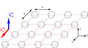
Figure 1: 2D square assembly of nano-spheres on a square super-lattice of parameter $a$ (same geometry as in Ref. [Déjardin et al., 2017]). The external DC field is applied along the $z$-axis, the AC field lies in the $xy$-plane. The assembly is monodisperse and textured with all anisotropy easy axes oriented in the $z$ direction.

In the present work, we consider the same system setup as in Ref. Déjardin et al., 2017, namely of oriented uniaxial anisotropy for all nanoparticles and a longitudinal DC magnetic field, in the intermediate–to-high damping regime, and in the high-anisotropy limit. In this case, the cubic contribution to the AC susceptibility is given by Eq. (37) of Ref. García-Palacios and Garanin, 2004, i.e.

$$\chi^{\left(3\right)}=\chi_{{\rm eq}}^{\left(3\right)}\frac{1-\frac{1}{2}i\eta}{\left(1+i\eta\right)\left(1+3i\eta\right)}$$ (3)

where

$$\chi_{{\rm eq},{\rm free}}^{\left(3\right)}=-\frac{1}{3}\frac{m^{4}}{\left(k_{B}T\right)^{3}}.$$

and $\eta=\omega\tau$, $\tau$ is the (longitudinal) Néel relaxation time, and $\chi_{{\rm eq}}^{\left(3\right)}$ is the cubic contribution to the equilibrium susceptibility. The high-energy barrier limit requires $\sigma=K_{{\rm eff}}V/k_{B}T\gg 1$, where $K_{{\rm eff}}$ is considered to be the largest energy scale in the present calculations and $k_{B}$ is the Boltzmann constant. This limit applies in the context of hyperthermia experiments (at temperature $T\simeq 318{\rm K}$). Indeed, for iron-cobalt nanoparticles of volume $V\sim 5.23\times 10^{-25}{\rm m^{3}}$ (i.e. spheres of radius $R=5\ {\rm nm}$), with an effective anisotropy constant $K_{{\rm eff}}\sim 4.5\times 10^{4}{\rm J.m^{-3}}$ and a density $\rho\simeq 8300\ {\rm kg.m^{-3}}$, we have $\sigma\simeq 5.4$.

Taking account of dipolar interactions (DI) together with uniaxial anisotropy and DC magnetic field ($\bm{H}_{{\rm ex}}=H_{{\rm DC}}\bm{e_{z}}$), the energy of a magnetic moment $\bm{m}_{i}$ within the assembly, reads (after multiplying by $-\beta\equiv-1/k_{B}T$)(Déjardin et al., 2017)

$$\mathcal{E}_{i}=x\,{\bf s}_{i}\cdot\bm{e_{z}}+\sigma\left(\mathbf{s}_{i}\cdot\bm{e_{z}}\right)^{2}+{\cal E}_{i}^{\mathrm{DI}},$$ (4)

where $x=\beta mH_{{\rm DC}}$ and ${\cal E}_{i}^{\mathrm{DI}}$ is the contribution from the long-range DI,

$${\cal E}_{i}^{\mathrm{DI}}=\xi\sum_{j<i}{\bf s}_{i}\cdot{\cal D}_{ij}\cdot{\bf s}_{j},$$ (5)

with the usual notation: ${\cal D}_{ij}=\left(3\bm{e}_{ij}\bm{e}_{ij}-1\right)/r_{ij}^{3}$, $\bm{r}_{ij}=\bm{r}_{i}-\bm{r}_{j}$, $r_{ij}=\left|\bm{r}_{ij}\right|,\bm{e}_{ij}=\bm{r}_{ij}/r_{ij}$. For convenience, we also use the dimensionless DI coefficient $\xi$

$$\xi=\left(\frac{\mu_{0}}{4\pi}\right)\left(\frac{m^{2}/a^{3}}{k_{B}T}\right).$$ (6)

In summary, the variable energy parameters of our calculations are $\xi$ and $x$, in addition to the AC field amplitude $H_{0}$ ; the frequency $\omega=2\pi f$ of the latter and the remaining parameters will be held constant. We will adopt a perturbative approach to derive analytical expressions for the SAR as a function of $\xi,x,H_{0}$ and use them to investigate the effect of $x,\xi$, as we vary $H_{0}$ in the wide range explored by experiments.

III AC Susceptibility

The AC susceptibility is a complex quantity that can be written as $\chi\left(x,\sigma,\xi,\omega\right)=\chi^{\prime}-i\chi^{\prime\prime}$. As usual, it can be expanded in terms of the amplitude $H_{0}$ of the AC field(Raikher and Stepanov, 1997)

$$\chi = \chi^{\left(1\right)}+3H_{0}^{2}\chi^{\left(3\right)}+\ldots\ .$$ (7)

$\chi^{\left(1\right)}$ is the linear contribution which, according to the model of Debye, reads

$$\chi^{\left(1\right)}=\chi_{\mathrm{eq}}^{\left(1\right)}\frac{1}{1+i\eta},$$ (8)

where $\chi_{\mathrm{eq}}^{\left(1\right)}$ is the equilibrium susceptibility. According to the Debye theory(Debye, 1929; Zwanzig, 1963) the only interaction of the molecule (here a nanoparticle) is with the external field. In the context of magnetic nanoparticles, this theory describes the absorption by a single mode of the electromagnetic energy brought in by the external field. In the case of weak inter-particle interactions, the dynamics of this mode is rather slow and characterized by the longitudinal relaxation time $\tau$, corresponding to the population inversion from the blocked state to the superparamagnetic state. The latter transition corresponds on average to the crossing by each nanoparticle’s magnetic moment of its energy barrier. As argued in Ref. Zwanzig, 1963, dipolar interactions introduce new relaxation times in higher-order perturbation theory and are associated with further losses at higher frequencies. However, in the hyperthermia context, the magnetic field frequency $\omega$ is relatively low (a few hundred kHz) and as such the Debye approximation with the first term in Eq. (8) is sufficient. On the other hand, the corrections due to (weak) dipolar interactions can be taken into account through the equilibrium susceptibility $\chi_{\mathrm{eq}}^{\left(1\right)}$, see Eqs. (11), (14) and (15) in Ref. Déjardin et al., 2017, within the limit of small DC field and linear equilibrium susceptibility. More precisely, we introduced $\chi_{{\rm eq,free}}$ the “free” contribution for a single particle and the interacting contribution $\chi_{{\rm eq,int}}$ to the equilibrium suceptibility, and therefore wrote

$$\chi_{\mathrm{eq}}^{\left(1\right)}=\chi_{{\rm eq,free}}^{\left(1\right)}+\tilde{\xi}\chi_{{\rm eq,int}}^{\left(1\right)},$$ (9)

where $\tilde{\xi}=\xi\mathcal{C}^{\left(0,0\right)}$, is the genuine coefficient that accounts for the DI intensity $\xi$ and the super-lattice through the lattice sum $\mathcal{C}^{\left(0,0\right)}$ which evaluates to $\mathcal{C}^{\left(0,0\right)}\simeq-9$ for the square sample shown in Fig. 1. All the details of the analytical expressions of these various quantities are available in Ref. Déjardin et al., 2017 and will not be reproduced here.

In the linear regime with respect to the AC magnetic field, i.e. restricting the expansion in Eq. (7) to the first term, the SAR was computed in Ref. Déjardin et al., 2017 as a function of the DC magnetic field and assembly concentration, see Fig. 6 therein. Now, we extend the expansion one step further and include the second term with the cubic susceptibility $\chi^{\left(3\right)}$ given by (3). Consequently, the general expression of the SAR in Eq. (2) can then be regarded as a double expansion: i) an expansion to second order in terms of the magnitude $H_{0}$ of the AC magnetic field (thus bringing the linear and cubic susceptibilities, i.e. $\chi^{\left(1\right)}$ and $\chi^{\left(3\right)}$), and ii) an expansion in the DI strength $\tilde{\xi}$ for the equilibrium susceptibilities ($\chi_{\mathrm{eq}}^{\left(1\right)}$ and $\chi_{\mathrm{eq}}^{\left(3\right)}$). So, in principle one should perform the latter expansion for both $\chi_{\mathrm{eq}}^{\left(1\right)}$ and $\chi_{\mathrm{eq}}^{\left(3\right)}$. However, writing $\chi_{{\rm eq}}^{\left(3\right)}=\chi_{{\rm eq,free}}^{\left(3\right)}+\tilde{\xi}\chi_{{\rm eq,int}}^{\left(3\right)}$, similarly to Eq. (9), leads to ($\Im$ stands for imaginary part)

$${\rm SAR} \simeq\frac{\mu_{0}\omega}{2\pi}H_{0}^{2}\Im\left[\chi_{{\rm free}}^{\left(1\right)}+\tilde{\xi}\chi_{{\rm int}}^{\left(1\right)}+3H_{0}^{2}\left(\chi_{{\rm free}}^{\left(3\right)}+\tilde{\xi}\chi_{{\rm int}}^{\left(3\right)}\right)\right]$$

$$={\rm SAR}^{\left(1\right)}+\frac{3\mu_{0}\omega}{2\pi}H_{0}^{4}\Im\left(\chi_{{\rm free}}^{\left(3\right)}+\tilde{\xi}\chi_{{\rm int}}^{\left(3\right)}\right)$$ (10)

where ${\rm SAR}^{\left(1\right)}$ is the SAR involving only the linear susceptibility studied in Ref. Déjardin et al., 2017.

However, we note that at low fields, as it is clearly seen in both the experimental(Bitoh et al., 1995, 1996) and theoretical (Raikher and Stepanov, 1997) results, the imaginary part of $H_{0}^{2}\chi_{{\rm free}}^{\left(3\right)}$ is at least one order of magnitude smaller than that of $\chi_{{\rm eq,free}}^{\left(1\right)}$ (in absolute value), and $\tilde{\xi}\chi_{{\rm int}}^{\left(3\right)}$ is even smaller. The calculation of the latter is rather involved and would require, for instance, the generalization of the work by Raihker and Stepanov(Raikher and Stepanov, 1997) for noninteracting particles in order to include dipolar interactions, or the extension of the work by Jönsson and García-Palacios to dynamic susceptibility. However, the aim of the present work is not to investigate concentrated samples, but to determine the general tendency implied by the effects of assemblies on SAR. For these reasons, we focus on low-values of $\xi$ and neglect higher-order corrections in $\tilde{\xi}\chi_{{\rm int}}^{\left(3\right)}$. In fact, we think that it is worth investigating the effect of the cubic AC susceptibility already through its “free” contribution $\chi_{{\rm free}}^{\left(3\right)}$, remembering that, at any rate, the whole approach assumes weak DI. In conclusion, we will compute the following correction to the SAR

$${\rm SAR}^{\left(3\right)}\simeq\frac{3\mu_{0}\omega}{2\pi}H_{0}^{4}\Im\left[\chi_{{\rm free}}^{\left(3\right)}\right]$$ (11)

where $\chi_{{\rm free}}^{\left(3\right)}$ is given by Eq. (3).

More explicitly, we obtain

$${\rm SAR}^{\left(3\right)} =\frac{3\mu_{0}m^{4}}{4\pi\left(k_{B}T\right)^{3}}H_{0}^{4}\frac{\left(3-\eta^{2}\right)\eta^{2}/\tau}{\left(\eta^{2}+1\right)\left(9\eta^{2}+1\right)}.$$ (12)

IV Results and discussion

The physical parameters used in the following are basically the same as those used in our earlier work(Déjardin et al., 2017) and have been recalled in Section II. The DC field is oriented along the anisotropy axis, i.e. perpendicular to the plane, with a normalized magnitude $h=x/2\sigma$.

We decided to focus our investigation on solid samples, with nanoparticles on the vertices of a square lattice. Other sample geometries could be investigated by computing the appropriate lattice sum $\mathcal{C}^{\left(0,0\right)}$, even non-periodic systems can be tackled by randomly depleting the initial sample. However, in such samples, the main effect would then be to effectively modulate the dipolar field by changing the value of $\tilde{\xi}$. The impact of the nonlinearities in these systems would remain the same since the correction in $\tilde{\xi}\chi_{{\rm int}}^{\left(3\right)}$ are of higher-order in comparison to the free contribution. On the other hand, as discussed earlier, the study of samples with solid matrices makes it possible to simplify the problem by avoiding extra degrees freedom and related loss sources (Brownian motion and field-induced stirring). This is necessary for a more precise and conclusive study of heating due to susceptibility losses, especially for small nanoparticles for which the latter dominate(Vallejo-Fernandez et al., 2013). In addition, this simplification helps investigate, in a somewhat pure form, nonlinear effects of magnetization processes induced by an increasing AC field.

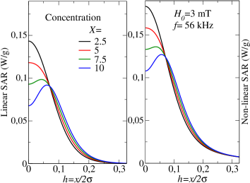
Figure 2: Left panel: linear SAR (${\rm SAR^{\left(1\right)}}$) as a function of the DC field for a 2D sample, for different concentrations $X$. Right panel: nonlinear SAR (${\rm SAR}={\rm SAR^{\left(1\right)}}+{\rm SAR^{\left(3\right)}}$). For both panels the AC field intensity is $H_{0}=3\ {\rm mT}$ and frequency $f=56\ {\rm kHz}$.

The first term of expression (10), i.e. ${\rm SAR^{\left(1\right)}}$, the linear susceptibility contribution, is plotted on the left panel of Fig. 2 against the DC field for different concentrations $X=10^{-21}/a^{3}$ , where the lattice parameter $a$ is expressed in meters, so an inter-particle separation of 46 nm corresponds to $X\sim 10$. The right panel of Fig. 2 displays the behavior of the SAR as expressed in Eq. (10) which includes the first nonlinear correction to the susceptibility given in Eq. (12). From a quantitative point of view, one can see that the SAR is slightly enhanced by the nonlinear correction. This is due to the fact that while ${\rm SAR^{\left(1\right)}}$ scales like $H_{0}^{2}$, ${\rm SAR^{\left(3\right)}}$ has a quartic behavior in terms of the AC field intensity. In the present case, with such a relatively low AC field intensity ($H_{0}=3\ {\rm mT}$), neither the quantitative nor the qualitative behavior is notably modified: at low DC field, for such a square sample, the SAR is reduced by the DI which compete with the anisoptropy and thus soften the whole magnetic system. This competition also leads to a non-monotonic behavior of the SAR as a function of $h$ and a crossing of the curves, as discussed in a previous work.(Déjardin et al., 2017) This result shows that the nonlinear correction to the SAR does not alter our conclusion that in some specific situations, the SAR may be optimized by applying an external DC field.

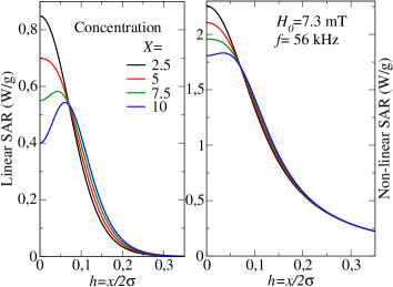
Figure 3: Same parameters as in Fig. 2, but for a higher AC field intensity $H_{0}=7.3{\rm\ mT}$.

The two different scaling laws, ${\rm SAR^{\left(1\right)}}\propto H_{0}^{2}$ and ${\rm SAR^{\left(3\right)}}\propto H_{0}^{4}$, suggest that one should be careful when using Eq. (10) to compute the SAR for higher AC fields. In Fig. 3 we plot ${\rm SAR^{\left(1\right)}}$ and ${\rm SAR}={\rm SAR^{\left(1\right)}}+{\rm SAR^{\left(3\right)}}$ for $H_{0}=7.3{\rm\ mT}$. By comparing the left panels of Figs. 2 and 3, which display ${\rm SAR^{\left(1\right)}}$ for the two different AC field amplitudes, 3 mT and 7.3 mT, we see that the curves are exactly the same but merely rescaled by a global factor $\left(7.3/3\right)^{2}$. This is in contrast with the respective right panels: upon including the cubic correction in the susceptibility, the simple scaling no longer applies. Indeed, a comparison of the left and right panels of Fig. 3 shows that while the qualitative behavior remains the same, the SAR is greatly enhanced by the correction ${\rm SAR^{\left(3\right)}}$. This hints at the fact that it might be necessary to consider even higher order terms [see Ref. F. Vernay and J.-L. Déjardin and H. Kachkachi, Efficiency of energy dissipation in nanomagnets: a theoretical study of ac susceptibility, 2020].

On the other hand, this addresses another issue regarding the critical product Brezovich, 1988 $H_{0}f\simeq 4.85\times 10^{8}\,{\rm A.m^{-1}.s^{-1}}$, considered as a physiological limit. From the physicist standpoint, this limit should be considered as an approximation of a more general condition. Indeed, the expansion of Eq. (10) can formally be rewritten as ${\rm SAR}\propto\left(H_{0}f\right)^{2}\left(1+\alpha H_{0}^{2}\right)$, which thus shows that the product $H_{0}f$ is only relevant at very low field intensities. Consequently, our results confirm the physiological argument when the quadratic regime dominates the SAR. To illustrate this, in Fig. 4 we plot the linear and nonlinear SAR as a function of $H_{0}$ for two different concentrations. In this log-log plot, the linear SAR exhibits, as expected, a linear behavior, while the nonlinear SAR shows a crossover between a quadratic (same slope as ${\rm SAR^{\left(1\right)}}$) and a quartic behavior for higher fields. The slope rapidly changes and hardens as $H_{0}$ increases, with a correction that becomes very large near $H_{0}=7{\rm\ mT}$, suggesting that higher order terms should become dominant. This particular value of $H_{0}$ can be understood upon inspecting the relative equilibrium susceptibilities at orders 1 and 3, since they roughly give the orders of magnitudes of $\chi^{\left(1\right)}$ and $\chi^{\left(3\right)}$, as can be seen in Eqs. (3) and (8). The remaining terms of these equations are related to the dynamics with the imaginary parts scaling as $\sim\eta$ in both cases. A rough estimate of the critical AC field value for which the ${\rm SAR}$ goes to a quartic behavior, may be inferred from the condition $H_{0}^{2}\left|\chi_{{\rm eq,free}}^{\left(3\right)}/\chi_{{\rm eq,free}}^{\left(1\right)}\right|\apprle 1$. This leads to $H_{0,c}\sim\frac{k_{B}T}{\mu_{0}m}$ which, for the present sample evaluates to $7.2{\rm\ mT}$ and thereby $H_{0,c}f\simeq 3.2\times 10^{8}{\rm A.m^{-1}.s^{-1}}$.

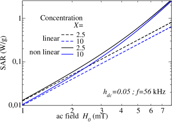
Figure 4: Log-Log plot of the linear and nonlinear SAR as a function of the AC field intensity for two different concentrations $X=2.5$ and 10, a fixed frequency and a finite DC field $h=0.05$.

For fields below $H_{0,c}$, a criterion based on the quantity $\left(H_{0}f\right)^{2}$ makes sense both from a physiological and a physical point of view. According to Eq. (2) the ${\rm SAR}$ is equal to $H_{0}^{2}f$ multiplied by a contribution from the imaginary part of the susceptibility $\chi^{\prime\prime}$. In terms of frequency, the latter scales with $f$ at all orders of the expansion and, in terms of the field intensity, the correction of order $\left(2n+1\right)$ scales with $H_{0}^{2n}$. Altogether, this implies that for fields below $H_{0,c}$ the expansion is dominated by the first order, and thus ${\rm SAR}\sim\mu_{0}\left(H_{0}f\right)^{2}$. This has been checked by investigating the ${\rm SAR}$ as a function of the frequency in Fig. 5. For $H_{0}=3{\rm\ mT}$, the linear and non linear SAR are qualitatively and quantitatively close and they both exhibit a $f^{2}$ behavior since both $\Im\left[\chi^{\left(1\right)}\right]$ and $\Im\left[\chi^{\left(3\right)}\right]$ are proportional to the frequency.

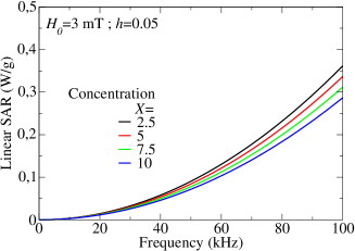
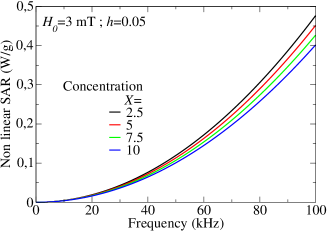
Figure 5: Linear and nonlinear SAR as a function of the AC field frequency for two different concentrations, for a fixed AC field intensity $H_{0}=3{\rm\ mT}$ and a finite DC field $h=0.05$.

V Conclusion

In the present investigation we have expressed the specific absorption rate (SAR) in terms of the out-of-phase of the dynamical susceptibility and have thereby provided analytical formulae that account for intrinsic and collective effects, as well as the first nonlinear correction to the AC susceptibility. In particular, the competition between the DC field and dipolar interactions which, according to our previous study, leads to a nonmonotonous behavior for the SAR, carries over, at least qualitatively, to the nonlinear regime for the AC field intensity. This implies that the DC field, even in the regime of higher AC field intensities, remains a key parameter for optimizing the SAR for such $2D$ arrays of nanomagnets.

Incidentally, we discussed applications to hyperthermia and the corresponding (physiological) upper limit on the product $H_{0}f$. We have seen that nonlinear contributions to the SAR bring an extra dependence on the AC field intensity and frequency. As a consequence, it is more relevant, from the physical point of view, and as long as the SAR is used for assessing the efficiency of magnetic hyperthemia, to consider instead the factor $\left(H_{0}f\right)^{2}$with which the SAR globally scales.

Data Availability

The data that support the findings of this study are available from the corresponding author upon reasonable request.

References

- Carrey, Mehdaoui, and Respaud (2011) J. Carrey, B. Mehdaoui, and M. Respaud, Journal of Applied Physics 109, 083921 (2011), 10.1063/1.3551582.
- Mehdaoui et al. (2011) B. Mehdaoui, A. Meffre, J. Carrey, S. Lachaize, L.-M. Lacroix, M. Gougeon, B. Chaudret, and M. Respaud, Advanced Functional Materials 21, 4573 (2011).
- Martinez-Boubeta et al. (2013) C. Martinez-Boubeta, K. Simeonidis, A. Makridis, M. Angelakeris, O. Iglesias, P. Guardia, A. Cabot, L. Yedra, S. Estradé, F. Peiró, et al., Scientific reports 3, 1652 (2013).
- Conde-Leboran et al. (2015) I. Conde-Leboran, D. Baldomir, C. Martinez-Boubeta, O. Chubykalo-Fesenko, M. d. P. Morales, G. Salas, D. Cabrera, J. Camarero, F. J. Teran, and D. Serantes, The Journal of Physical Chemistry C 119, 15698 (2015).
- Kostopoulou and Lappas (2015) A. Kostopoulou and A. Lappas, Nanotechnology Reviews 4, 595 (2015).
- Shah et al. (2015) R. R. Shah, T. P. Davis, A. L. Glover, D. E. Nikles, and C. S. Brazel, Journal of Magnetism and Magnetic Materials 387, 96 (2015).
- Brezovich (1988) I. Brezovich, Med. Phys. Monogr. 16, 82 (1988).
- Glover et al. (2013) A. L. Glover, J. B. Bennett, J. S. Pritchett, S. M. Nikles, D. E. Nikles, J. A. Nikles, and C. S. Brazel, IEEE Transactions on Magnetics 49, 231 (2013).
- Bordelon et al. (2011) D. E. Bordelon, C. Cornejo, C. Gruttner, F. Westphal, T. L. DeWeese, and R. Ivkov, Journal of Applied Physics 109, 124904 (2011), https://doi.org/10.1063/1.3597820 .
- Murase et al. (2011) K. Murase, J. Oonoki, H. Takata, R. Song, A. Angraini, P. Ausanai, and T. Matsushita, Radiological Physics and Technology 4, 194 (2011).
- Gonzales-Weimuller, Zeisberger, and Krishnan (2009) M. Gonzales-Weimuller, M. Zeisberger, and K. M. Krishnan, Journal of Magnetism and Magnetic Materials 321, 1947 (2009).
- Guardia et al. (2012) P. Guardia, R. Di Corato, L. Lartigue, C. Wilhelm, A. Espinosa, M. Garcia-Hernandez, F. Gazeau, L. Manna, and T. Pellegrino, ACS Nano 6, 3080 (2012).
- Lacroix et al. (2009) L.-M. Lacroix, R. B. Malaki, J. Carrey, S. Lachaize, M. Respaud, G. F. Goya, and B. Chaudret, Journal of Applied Physics 105, 023911 (2009).
- Mehdaoui et al. (2012) B. Mehdaoui, J. Carrey, M. Stadler, A. Cornejo, C. Nayral, F. Delpech, B. Chaudret, and M. Respaud, Appl. Phys. Lett. 100, 052403 (2012).
- L. D. Landau and E. M. Lifshitz (1960) L. D. Landau and E. M. Lifshitz, Electrodynamics of Continuous Media (Pergamon, London, 1960).
- Rosensweig (2002) R. Rosensweig, Journal of Magnetism and Magnetic Materials 252, 370 (2002), proceedings of the 9th International Conference on Magnetic Fluids, 23-27 Jul. 2001.
- Hergt et al. (2006) R. Hergt, S. Dutz, R. Müller, and M. Zeisberger, Journal of Physics Condensed Matter 18, 2919 (2006).
- Ahrentorp et al. (2010) F. Ahrentorp, A. P. Astalan, C. Jonasson, J. Blomgren, B. Qi, O. T. Mefford, M. Yan, J. Courtois, J.-F. Berret, J. Fresnais, O. Sandre, S. Dutz, R. Müller, and C. Johansson, AIP Conference Proceedings 1311, 213 (2010).
- Déjardin et al. (2017) J.-L. Déjardin, F. Vernay, M. Respaud, and H. Kachkachi, Journal of Applied Physics 121, 203903 (2017), https://doi.org/10.1063/1.4984013 .
- J.L. Garcia-Palacios (2007) J.L. Garcia-Palacios, “On the Statics and Dynamics of Magnetoanisotropic Nanoparticles,” in Advances in Chemical Physics, Vol. 112 (John Wiley & Sons, Inc., 2007) pp. 1–210.
- Vernay, Sabsabi, and Kachkachi (2014) F. Vernay, Z. Sabsabi, and H. Kachkachi, Phys. Rev. B 90, 094416 (2014).
- Bitoh et al. (1995) T. Bitoh, K. Ohba, M. Takamatsu, T. Shirane, and S. Chikazawa, Journal of the Physical Society of Japan 64, 1311 (1995), https://doi.org/10.1143/JPSJ.64.1311 .
- Bitoh et al. (1996) T. Bitoh, K. Ohba, M. Takamatsu, T. Shirane, and S. Chikazawa, Journal of Magnetism and Magnetic Materials 154, 59 (1996).
- Raikher and Stepanov (1997) Y. L. Raikher and V. I. Stepanov, Phys. Rev. B 55, 15005 (1997).
- Raikher and Stepanov (1999) Y. Raikher and V. Stepanov, Journal of Magnetism and Magnetic Materials 196-197, 88 (1999).
- P. Jönsson, T. Jonsson, J. L. Gacía-Palacios, P. Svedlindh (2000) P. Jönsson, T. Jonsson, J. L. Gacía-Palacios, P. Svedlindh, Journal of Magnetism and Magnetic Materials 222, 219 (2000).
- Raikher and Stepanov (2002) Y. L. Raikher and V. I. Stepanov, Phys. Rev. B 66, 214406 (2002).
- García-Palacios and Garanin (2004) J. L. García-Palacios and D. A. Garanin, Phys. Rev. B 70, 064415 (2004).
- Wang and Huang (2006) G. Wang and J. P. Huang, Chemical Physics Letters 421, 544 (2006).
- B. Ficko (2015) S. G. D. B. Ficko, P. Giacometti, Journal of Magnetism and Magnetic Materials 378, 267 (2015).
- Raikher and Stepanov (2008) Y. Raikher and V. Stepanov, Journal of Magnetism and Magnetic Materials 320, 2692 (2008).
- Vallejo-Fernandez et al. (2013) G. Vallejo-Fernandez, O. Whear, A. G. Roca, S. Hussain, J. Timmis, V. Patel, and K. O’Grady, Journal of Physics D: Applied Physics 46, 312001 (2013).
- Vallejo-Fernandez and O’Grady (2013) G. Vallejo-Fernandez and K. O’Grady, Applied Physics Letters 103, 142417 (2013), https://doi.org/10.1063/1.4824649 .
- Debye (1929) P. Debye, Polar molecules (Dover, 1929).
- Zwanzig (1963) R. Zwanzig, The Journal of Chemical Physics 38, 2766 (1963).
- F. Vernay and J.-L. Déjardin and H. Kachkachi, Efficiency of energy dissipation in nanomagnets: a theoretical study of ac susceptibility (2020) F. Vernay and J.-L. Déjardin and H. Kachkachi, Efficiency of energy dissipation in nanomagnets: a theoretical study of ac susceptibility, in Magnetic Nanoparticles in Human Health and Medicine, Vol. xxx, edited by M. Rai and C. Caizer (SPRINGER-VERLAG, 2020) p. xxx.