Learning the Redundancy-free Features for Generalized Zero-Shot Object Recognition

Abstract

Zero-shot object recognition or zero-shot learning aims to transfer the object recognition ability among the semantically related categories, such as fine-grained animal or bird species. However, the images of different fine-grained objects tend to merely exhibit subtle differences in appearance, which will severely deteriorate zero-shot object recognition. To reduce the superfluous information in the fine-grained objects, in this paper, we propose to learn the redundancy-free features for generalized zero-shot learning. We achieve our motivation by projecting the original visual features into a new (redundancy-free) feature space and then restricting the statistical dependence between these two feature spaces. Furthermore, we require the projected features to keep and even strengthen the category relationship in the redundancy-free feature space. In this way, we can remove the redundant information from the visual features without losing the discriminative information. We extensively evaluate the performance on four benchmark datasets. The results show that our redundancy-free feature based generalized zero-shot learning (RFF-GZSL) approach can achieve competitive results compared with the state-of-the-arts.

1 Introduction

Object recognition has progressed remarkably in recent years thanks to the deployments of deep Convolutional Neural Networks (CNNs) [24, 18]. However, existing CNN-based models, with tens to hundreds of millions of parameters, excel only when large amounts of labeled data are available for each object class, and generally struggle when labeled data are scarce. The data-hungry nature of deep models limits their ability to recognize rare object classes, such as fine-grained animal species. This is because collecting and annotating a large set of images of these classes is often labor-intensive and sometimes impossible (e.g., extinct species). Zero-Shot Learning (ZSL), also known as learning from side information, provides a promising approach to addressing this problem [26, 40]. Specifically, zero-shot learning aims to recognize the unseen classes, of which the labeled images are unavailable, when the labeled images only from some seen classes are provided [27, 54]. In ZSL, the seen classes are associated with the unseen classes in a semantic descriptor space, such as the semantic attribute or word vector space [2], which bridges the knowledge gap between the seen and unseen classes.

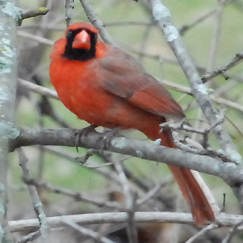
(a) Cardinal

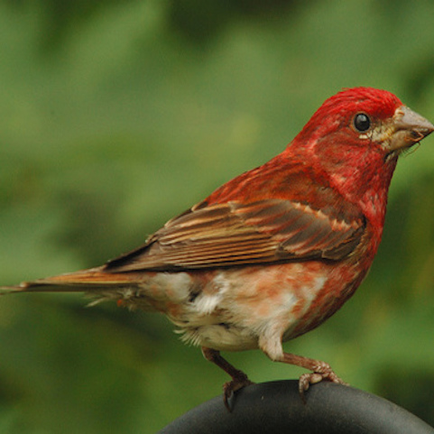
(b) Purple finch

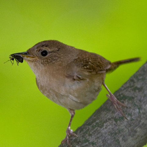
(c) House wren

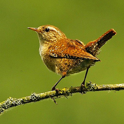
(d) Winter wren

Figure 1: Examples of four fine-grained bird species. The subtle difference in appearance or the common living environment of these examples challenges the zero-shot object recognition.

Although the conventional ZSL prevails in the early researches, the realistic but more challenging Generalized Zero-Shot Learning (GZSL) has drawn increasing attention recently. The conventional ZSL assumes all test images coming from the unseen classes only, whereas the test set in GZSL consists of data from both the seen and unseen classes. Semantic embedding is the most important approach in conventional ZSL, but generally performs poor in the new GZSL setting. The semantic embedding methods [13, 27, 2] learn to embed the visual features into the semantic descriptor space and then predict the labels of visual features by finding their nearest semantic descriptor. In GZSL, to mitigate the data imbalance between seen and unseen classes, a number of feature generation methods have been proposed [53, 25, 12, 48, 55]. The feature generation methods first learn a feature generator network conditioned on the class-level semantic descriptors. The feature generator can produce an arbitrary number of synthetic features and thus compensate for the lack of visual features for the unseen classes. In the end, the feature generation methods mix the real seen features and the fake unseen features to train a supervised model, e.g. a softmax classifier, as the final GZSL classifier.

Generalized zero-shot learning is usually evaluated on the fine-grained datasets, such as Caltech-UCSD Birds (CUB) [50], as the fine-grained categories are semantically related. The images of different fine-grained categories tend to be very similar in appearance and merely exhibit subtle differences, which will severely deteriorate the performance of the GZSL classification. A similar background, such as a common living environment, of fine-grained animal or bird species may also mislead the zero-shot object recognition on these datasets, as shown in Figure 1. In other words, the fine-grained images in GZSL contain superfluous content irrelevant to differentiating their categories. Intuitively, GZSL can benefit from removing the redundancy from the original visual features and preserving the most discriminative information that triggers a class label.

In this paper, we present a generalized zero-shot learning approach based on redundancy-free information. Specifically, we propose to map the original visual features into a new space, where we bound the dependence between the mapped features and the visual features to remove the redundancy from the visual features. In the meanwhile, we minimize the generalized ZSL classification error using the new redundancy-free features to keep the discriminative information in it. Our method is flexible in that it can be integrated with the two aforementioned frameworks, i.e. semantic embedding and feature generation, for GZSL. We evaluate our method on four widely used datasets. The results show that when integrating with the conventional semantic embedding framework, our model can surpass the other conventional ZSL comparators in the new GZSL setting; when integrating with the feature generation framework, to the best of our knowledge, our model can achieve the state-of-the-art on two datasets and competitive results on the other two datasets. This suggests that the redundancy-free features are effective for the GZSL task.

Our contributions are three-fold: (1) we propose a redundancy-free feature based GZSL method; (2) our method can integrate with the conventional semantic embedding and the latest feature generation frameworks; and (3) we evaluate our GZSL model on four benchmarks, and to the best of our knowledge, our method can achieve the state-of-the-art or competitive results on these benchmarks.

1.1 Related Work

Zero-shot object recognition or zero-shot learning relies on the class-level semantic descriptions or features, e.g. semantic attributes [11, 41, 2] and word vectors [34, 35], for model transferring from the seen classes to a disjoint set of unseen classes. Earlier ZSL research works focus on the conventional ZSL problem [38, 49, 13, 2, 58, 14, 22, 7, 52, 15, 9, 46, 23], in which the semantic embedding is the most important approach [13, 46, 7, 23]. Semantic embedding methods learn to embed the visual features into the semantic descriptor space, or vice versa [13, 1, 2, 23]. By doing so, the visual features and the semantic features will lie in a same space and the ZSL classification can be accomplished by searching the nearest semantic descriptor.

In the more challenging GZSL task, we have the labeled data only from seen classes during training, but need to recognize the images from both seen and unseen classes in the test phase. Thus, GZSL suffers from the extreme data imbalance problem. Semantic embedding methods fail to solve the data imbalance problem in GZSL. They tend to be highly overfitting the seen classes and thus harm the classification of unseen classes. The experiments in [54] showed that the performance of almost all conventional ZSL methods, including semantic embedding, drops significantly in the new GZSL scenario.

To compensate for the lack of training images of unseen classes in GZSL, recently, some feature generation methods have been proposed to tackle the GZSL problem [8, 53, 12, 25, 55, 19, 48]. Bucher et al. [8] proposed to generate features for unseen classes with four different generative models, including generative moment matching network (GMMN) [30], auxiliary classifier GANs (AC-GAN) [39], denoising auto-encoder [6] and adversarial auto-encoder (AAE) [33]. The f-CLSWGAN in [53] proposed to generate the unseen features conditioned on the class-level semantic descriptors. Some methods [12, 19] further constrained the feature generator network by introducing a reverse regressor network which can be used to define a cycle-consistent loss [59]. Verma et al. [25] built their feature synthesis framework upon Variational Autoencoder (VAE) [21]. Besides the feature generation methods, Chen et al. [10] proposed an adversarial visual-semantic embedding framework. Liu et al. [31] proposed a deep calibration network (DCN) that simultaneously calibrates the model confidence on seen classes and the model uncertainty on unseen classes.

As previously analyzed, the images of different fine-grained categories in GZSL differ slightly in appearance, which will challenge the GZSL classification. To mitigate this problem, we propose to reduce the redundant information in the visual features for GZSL. Our work is inspired by the information bottleneck method [3]. Concretely, we map the visual features into a new redundancy-free feature space and limit the information dependence between the mapped features and the original images features to an upper bound.

2 Preliminaries

In this section, we define the GZSL problem and then briefly revisit the semantic embedding and feature generation frameworks in GZSL.

Problem definition

In zero-shot learning, we are given a set of seen classes $\mathcal{Y}_{s}$ and a disjoint set of unseen classes $\mathcal{Y}_{u}$, where we have $\mathcal{Y}_{s}\cap\mathcal{Y}_{u}=\varnothing$. Suppose that there is a training dataset $\mathcal{D}^{tr}_{s}=\{(x_{i},a_{i},y_{i})\}$ consisting of labeled samples from the seen classes only, where $x_{i}\in X$ represents the visual feature, $a_{i}\in\mathcal{A}$ is the associated semantic descriptor (e.g. semantic attributes), and $y_{i}\in\mathcal{Y}_{s}$ denotes the seen class label. The semantic features of unseen classes are also available, but their visual features are missing. Zero-shot learning aims to learn a classifier being evaluated on a test dataset $\mathcal{D}^{te}=\{x_{k}\}$. In generalized ZSL, the test dataset $\mathcal{D}^{te}$ is composed of examples from both seen and unseen classes, i.e., GZSL is tested on $\mathcal{Y}_{s}\cup\mathcal{Y}_{u}$.

Semantic embedding

The conventional semantic embedding methods in ZSL learn an embedding function $E$ that maps a visual feature $x$ into the semantic descriptor space as $E(x)$. In this paper, we adopt a structured objective proposed in [2, 13] to learn the embedding function $E$. Such a structured objective requires the embedding of $x$ being closer to the semantic descriptor $a$ of its ground-truth class than the descriptors of other classes, according to the dot-product similarity in semantic descriptor space. This objective for learning $E$ is defined as below:

$$\min_{E}\mathbb{E}_{p(x,a)}[\max(0,\Delta-a^{\top}E(x)+(a^{\prime})^{\top}E(x))],$$ (1)

where $p(x,a)$ is the empirical data distribution of seen classes defined on $\mathcal{D}^{tr}_{s}$, $a^{\prime}\neq a$ is a randomly-selected semantic descriptor of other classes, and $\Delta>0$ is a margin to make $E$ more robust. Once the embedding function $E$ is optimized, we can use $E$ to embed the visual feature of a test image to the semantic descriptor space and infer its class label by finding the nearest semantic descriptor.

Feature generation

Semantic embedding methods prevail in the conventional ZSL but is unsuccessful in the more challenging generalized ZSL problem. Feature generation can address the data imbalance problem in GZSL and their effectiveness for GZSL has been evidenced recently [53, 25, 36, 19, 5]. We adopt a basic feature generation method, f-CLSWGAN, proposed in [53], although our approach based on redundancy-free features can certainly integrate with other more sophisticated feature generation methods. f-CLSWGAN learns a visual feature generator $G$, defined as a conditional generative model $\tilde{x}=G(a,\epsilon)$, conditioned on a semantic descriptor $a$ and a Gaussian noise $\epsilon\sim\mathcal{N}(\mathbf{0},\mathbf{I})$. In f-CLSWGAN, a discriminator $D$ is learned together with $G$ to discriminate a real pair $(x,a)$ from a synthetic pair $(\tilde{x},a)$, whereas the feature generator $G$ tries to fool the discriminator $D$ by producing indistinguishable synthetic features. As shown in [16], such an idea can be formulated as the following adversarial objective:

$$\min_{G}\max_{D}\mathbb{E}_{p(x,a)}[\log D(x,a)]+\mathbb{E}_{p_{G}(\tilde{x})}[\log(1-D(\tilde{x},a))],$$ (2)

where $p_{G}$ is the distribution of synthetic visual features. To make the generated visual features more discriminative, f-CLSWGAN further constrains the generator $G$ with a supervised classification loss:

$$\mathcal{L}_{CLS}(G)=-\mathbb{E}_{p_{G}(\tilde{x})}[\log q(y|\tilde{x})],$$ (3)

where $q(y|\tilde{x})$ is a classifier that is pre-trained on the seen training set $\mathcal{D}^{tr}_{s}$. $q(y|\tilde{x})$ gives the probability of $\tilde{x}$ being predicted as the label $y$ inherited from the conditional semantic descriptor $a$. The feature generator $G$ can synthesize an arbitrary number of labeled features for unseen classes. As a result, we can transform GZSL to a standard supervised learning problem.

3 Methodology

In this section, we present how to learn the redundancy-free information and then describe how it can be integrated with the semantic embedding and the feature generation frameworks, respectively, to tackle the GZSL problem.

3.1 Learning the Redundancy-free Information

We learn a mapping function $M$ to map the original visual features to a new feature space. Our goal is to remove the redundancy information contained in the original feature $x$ through $M$; $z=M(x)$ represents the redundancy-free information of $x$. Let $X$ be the original features and $Z$ be the redundancy-free features. We hope to perform the GZSL task using the redundancy-free features rather than the original redundancy features. To the end, we bound the statistical dependence between $Z$ and $X$ to enforce $Z$ to forget the redundancy information in $X$. In information theory, the dependence between two random variables is measured by mutual information (MI) $I(Z;X)$, defined as $I(Z;X)=H(Z)-H(Z|X)$, where $H(Z)$ is the marginal entropy of $Z$ and $H(Z|X)$ is the conditional entropy of $Z$ with respect to $X$. Note that we do not intend to minimize the mutual information $I(Z;X)$ but ask it to be lower than an upper bound, such that some information in $X$ can still be conveyed to $Z$. Otherwise, $I(Z;X)=0$ means $Z$ and $X$ are statistically independent.

Calculating the mutual information with high dimension is intractable. We follow the strategy proposed by Alemi et al. [3] to use a variational upper bound of MI as a surrogate:

$$I(Z;X)\leq\mathbb{E}_{p(x)}[D_{KL}[p_{M}(z|x)\|r(z)]],$$ (4)

where $D_{KL}()$ is the Kullback-Leibler (KL) divergence, $p_{M}(z|x)$ is the conditional distribution of redundancy-free features $z$ conditioned on the original visual features $x$. $r(z)$ is the variational approximation to the marginal distribution of $z$. The variational upper bound can be estimated using the reparameterization trick [21]. By restricting this variational upper bound, we can implicitly constrain the mutual information between $Z$ and $X$. In this way, the mapping function $M$ can be learned to extract the redundancy-free information from $x$.

Only removing the redundancy information from the original visual features cannot guarantee a satisfactory GZSL result. Next, we will discuss how to preserve the discriminative information concerning GZSL, in $z$.

3.2 Redundancy-free Semantic Embedding for GZSL

To exploit the redundancy-free information in the semantic embedding methods, we simply regard the semantic descriptor space as the new feature space and request the function $M$ to map the original visual features into the semantic descriptor space, analogously to the conventional semantic embedding method described above. Therefore, we just constrain the structured objective defined in Eq. 1 with the bounded variational mutual information as below:

$$\min_{M} \hskip 4.5pt\mathbb{E}_{p(x,a)}[\mathbb{E}_{p_{M}(z|x)}[\max(0,\Delta-a^{\top}z+(a^{\prime})^{\top}z)]]$$ (5)

s.t. $$\hskip 4.5pt\mathbb{E}_{p(x)}[D_{KL}[p_{M}(z|x)\|r(z)]]\leq b,$$

where $b$ is the upper bound we impose. We apply the strategy described in [44] to optimize an unconstrained form of Eq. 5 derived by the method of Lagrange multiplier.

Figure 2 shows the schematic overview of the redundancy-free semantic embedding method. Our method differs from the traditional semantic embedding methods in that we restrict the embedding $z=M(x)$ to preserve the information in the original feature $x$ to an upper bound. More specifically, in Eq. 5, the information constraint determines how much information in $x$ will be conveyed to $z$, and the classification term decides whether the left information is discriminative for GZSL or not.

Figure 2: The structure of the redundancy-free semantic embedding framework for GZSL. We learn a mapping function $M$ to project a visual feature to the semantic descriptor space. We bound the statistical dependence measured by the mutual information between the mapped features and the original visual features to enforce $M$ to extract the redundancy-free information from the visual features.

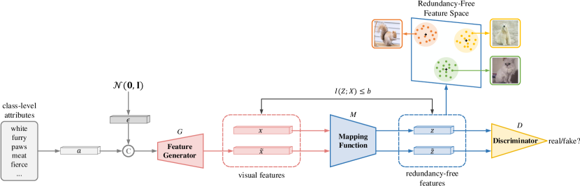
Figure 3: The structure of the redundancy-free feature generation framework for GZSL. We learn a feature generator $G$ that synthesizes the fake visual features for unseen classes using the class-level semantic descriptor $a$ (e.g. attributes) and a noise $\epsilon$. Furthermore, we learn a mapping function $M$ to map the real visual features of seen classes and the synthetic visual features of unseen classes into a new redundancy-free feature space. We remove the redundancy information from the visual features by restricting the mutual information between the original visual features and the redundancy-free features. Our redundancy-free features are discriminative for the GZSL task.

3.3 Redundancy-free Feature Generation for GZSL

Previous feature generation methods in GZSL trained a feature generator network to mimic the distribution of real visual features. To exploit the redundancy-free information in feature generation, we take one step further and learn a new mapping function $M$ to project the visual features, real and synthetic, to another feature space. For the seen classes in GZSL, we use the new mapping function $M$ to transform the original real visual features to the redundancy-free features: $z=M(x)$. For the unseen classes in GZSL, we indeed use a composite generator network $M\circ G$ to synthesize the fake and redundancy-free features: $\tilde{z}=(M\circ G)(a,\epsilon)=M(G(a,\epsilon))$. In this way, we can rewrite the adversarial objective of feature generation defined in Eq. 2 as follows:

$$V(D,M\circ G) =\mathbb{E}_{p(x)}[\mathbb{E}_{p_{M}(z|x)}[\log D(z)]]$$ (6)

$$\hskip 0.90005pt+\mathbb{E}_{p_{G}(\tilde{x})}[\mathbb{E}_{p_{M}(\tilde{z}|\tilde{x})}[\log(1-D(\tilde{z}))]],$$

where $p_{M}(\tilde{z}|\tilde{x})$ is the distribution of the synthesized redundancy-free features $\tilde{z}$ conditioned on the synthetic visual features $\tilde{x}$.

To ensure the generated features have a similar discriminative ability like the real feature, f-CLSWGAN further constrained the feature generator network $G$ with a pre-trained supervised classifier given in Eq. 3. Similarly, to ensure the redundancy-free features produced by $M$ are also discriminative, we use the training visual features of seen classes to constrain $M$ so that the category relationship of the seen training data can be well retained in the redundancy-free feature space. Concretely, we constrain the mapping function $M$ using the following loss objective:

$$\mathcal{L}_{r}(M,\mathbf{c})=\mathbb{E}_{p(x,y)}[\mathbb{E}_{p_{M}(z|x)}[\mathcal{L}_{c}(z,y,y^{\prime})]],$$ (7)

in which for each sample from seen classes, we compute the loss of its redundancy-free feature with the center loss proposed in [51] as below:

$$\mathcal{L}_{c}(z,y,y^{\prime})=\max(0,\Delta+\|z-\mathbf{c}_{y}\|^{2}_{2}-\|z-\mathbf{c}_{y^{\prime}}\|^{2}_{2}).$$ (8)

where $y$ is the class label of $x$ and $y^{\prime}$ is a randomly-selected class label other than $y$. In $\mathcal{L}_{r}(M,\mathbf{c})$, an array of centers in the redundancy-free feature space, one for each seen class, are optimized with $M$ together. The center loss can group the redundancy-free features of seen classes according to their labels such that the distributions of different classes can be easily separated. As such, we indeed strengthen the category relationships of seen class data in the new redundancy-free feature space.

We formulate our final learning objective for redundancy-free feature generation as follows:

$$\min_{G,M,\mathbf{c}}\max_{D} \hskip 2.70003ptV(D,M\circ G)+\lambda_{r}\mathcal{L}_{r}(M,\mathbf{c})+\lambda_{c}\mathcal{L}_{CLS}(G)$$ (9)

s.t. $$\hskip 2.70003pt\mathbb{E}_{p(x)}[D_{KL}[p_{M}(z|x)\|r(z)]]\leq b$$

$$\hskip 2.70003pt\mathbb{E}_{p_{G}(\tilde{x})}[D_{KL}[p_{M}(\tilde{z}|\tilde{x})\|r(\tilde{z})]]\leq b.$$

In Eq. 9, we learn the discriminator $D$ and the composite generator $M\circ G$ in an adversarial manner, to avoid the mismatching between the distribution of synthetic redundancy-free features and that of real redundancy-free features. We keep the classification loss $\mathcal{L}_{CLS}$ (Eq. 3) in the original visual feature space, to ensure the discriminative ability of the generated unseen visual features, which will be mapped to the new redundancy-free feature space later. The two information constraints bound the variational mutual information so that the redundancy information can be removed from the visual features. Last, $\mathcal{L}_{r}$ will encourage $M$ to produce the well-separated thus strongly discriminative redundancy-free features. Figure 3 shows the overall structure of the redundancy-free feature generation framework.

3.4 Classification

Semantic embedding

For a test data point $x\in\mathcal{D}^{te}$, we use $M$ to map it into the semantic descriptor space as $M(x)$. $x$ will be labeled as the class with the nearest semantic descriptor with respect to $x$:

$$y^{*}=\arg\max_{a\in\mathcal{A}_{s}\cup\mathcal{A}_{u}}a^{\top}M(x).$$ (10)

Feature Generation

We first map all training data of seen classes into the redundancy-free feature space as $z=M(x)$ for each $x\in D^{tr}_{s}$. We then synthesize a set of redundancy-free features for each unseen class $y\in\mathcal{Y}_{u}$ by performing $\tilde{z}=(M\circ G)(a_{y},\epsilon)$. Once we have the training data, real or fake for each seen or unseen class, we train a supervised classifier in the redundancy-free feature space as the final GZSL classifier. In this paper, we evaluate our method with softmax classifiers.

Table 1: Results of the state-of-the-arts. $U$ and $S$ are the Top-1 accuracies tested on unseen classes and seen classes, respectively, in GZSL. $H$ is the harmonic mean of $U$ and $S$. On each dataset, we synthesize different numbers of examples per unseen class: AWA (1800), CUB (400), SUN (400), and FLO (1200). ‡  and †  denote the feature generation methods or not, respectively. The best results and the second best results are respectively marked in bold and underlined.

	Method	AWA			CUB			SUN			FLO
		${U}$	${S}$	${H}$	${U}$	${S}$	${H}$	${U}$	${S}$	${H}$	${U}$	${S}$	${H}$
†	DCN [31]	25.5	84.2	39.1	28.4	60.7	38.7	25.5	37.0	30.2	-	-	-
	SP-AEN [10]	23.3	90.9	37.1	34.7	70.6	46.6	24.9	38.6	30.3	-	-	-
	AREN [56]	-	-	-	38.9	78.7	52.1	19.0	38.8	25.5	-	-	-
	Kai at el. [29]	62.7	77.0	69.1	47.4	47.6	47.5	36.3	42.8	39.3	-	-	-
	CRnet [57]	58.1	74.7	65.4	45.5	56.8	50.5	34.1	36.5	35.3	-	-	-
‡	SE-GZSL [25]	56.3	67.8	61.5	41.5	53.3	46.7	40.9	30.5	34.9	-	-	-
	f-CLSWGAN [53]	57.9	61.4	59.6	43.7	57.7	49.7	42.6	36.6	39.4	59.0	73.8	65.6
	cycle-CLSWGAN [12]	56.9	64.0	60.2	45.7	61.0	52.3	49.4	33.6	40.0	59.2	72.5	65.1
	CADA-VAE [48]	57.3	72.8	64.1	51.6	53.5	52.4	47.2	35.7	40.6	-	-	-
	SABR [43]	-	-	-	55.0	58.7	56.8	50.7	35.1	41.5	-	-	-
	f-VAEGAN [55]	-	-	-	48.4	60.1	53.6	45.1	38.0	41.3	56.8	74.9	64.6
	LisGAN [28]	52.6	76.3	62.3	46.5	57.9	51.6	42.9	37.8	40.2	57.7	83.8	68.3
	GMN [47]	61.1	71.3	65.8	56.1	54.3	55.2	53.2	33.0	40.7	-	-	-
	Our RFF-GZSL	59.8	75.1	66.5	52.6	56.6	54.6	45.7	38.6	41.9	65.2	78.2	71.1

4 Experiments

Datasets

We evaluate our method on four datasets for GZSL: (1) Animals with Attributes 1 (AWA) [26] consists of 50 classes of animals with 30,475 examples annotated with 85 attributes; (2) Caltech-UCSD Birds-200-2011 (CUB) [50] contains 11,788 examples of 200 fine-grained bird species annotated with 312 attributes; (3) SUN Attribute (SUN) [42] consists of 14,340 examples of 717 different scenes annotated with 102 attributes; (4) Oxford Flowers (FLO) [37] is composed of 8,189 examples of 102 different fine-grained flower classes annotated with 1,024 attributes [45]. We extract the 2,048-dimensional CNN features for images using ResNet-101 [18] as the visual features and the pre-defined attributes on each dataset are used as the semantic descriptors. Moreover, we adopt the Proposed Split (PS) [54] to divide the total classes into seen and unseen classes on each dataset.

Evaluation Protocols

The performances of our method are evaluated by per-class Top-1 accuracy. In GZSL, since the test set is composed of seen and unseen images, we will evaluate the Top-1 accuracies respectively on seen classes, denoted as $S$, and unseen classes, denoted as $U$. Their harmonic mean, defined as $H=(2\times S\times U)/(S+U)$ [54], evaluates the performance of GZSL.

Implementation Details

We implement our model with neural networks using PyTorch. The generator $G$ contains a 4096-unit hidden layer with LeakyReLU activation. The mapping function $M$ and discriminator $D$ is implemented with a fully-connected layer and ReLU activation. We use Adam solver [20] with $\beta_{1}=0.5,\beta_{2}=0.999$ and a batch size of 512. We empirically set the MI bound $b=0.1$, the dimension of redundancy-free feature space as 1,024 and $\lambda_{r}=0.1$; we cross-validate $\lambda_{c}$ in $[0.1,1]$. To make the training process more stable, we adopt Wasserstein GAN [4] and some improved strategies [17] in the feature generation framework.

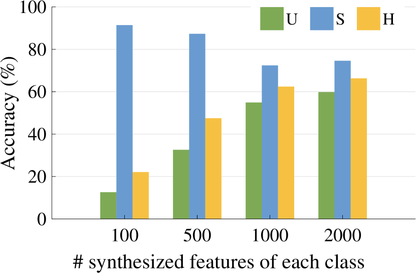
(a) AWA

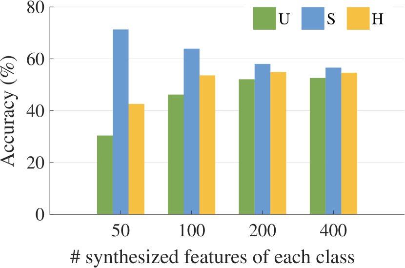
(b) CUB

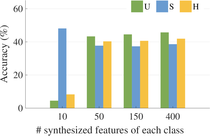
(c) SUN

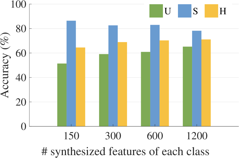
(d) FLO

Figure 4: The GZSL results of our RFF-GZSL with respect to different numbers of synthetic samples per unseen class.

Table 2: Results of comparison with traditional ZSL methods in the new GZSL scenario. $U$ and $S$ are the Top-1 accuracies tested on unseen classes and seen classes, respectively, in GZSL. $H$ is the harmonic mean of $U$ and $S$. The best results and the second best results are respectively marked in bold and underlined.

Method	AWA			CUB			SUN			FLO
	${U}$	${S}$	${H}$	${U}$	${S}$	${H}$	${U}$	${S}$	${H}$	${U}$	${S}$	${H}$
DAP [27]	0.0	88.7	0.0	1.7	67.9	3.3	4.2	25.1	7.2	-	-	-
IAP [27]	2.1	78.2	4.1	0.2	72.8	0.4	1.0	37.8	1.8	-	-	-
SJE [2]	11.3	74.6	19.6	23.5	59.2	33.6	14.7	30.5	19.8	13.9	47.6	21.5
LATEM [52]	7.3	71.7	13.3	15.2	57.3	24.0	14.7	28.8	19.5	6.6	47.6	11.5
DEVISE [13]	13.4	68.7	22.4	23.8	53.0	32.8	16.9	27.4	20.9	9.9	44.2	16.2
ALE [1]	16.8	76.1	27.5	23.7	62.8	34.4	21.8	33.1	26.3	13.3	61.6	21.9
ESZSL [46]	6.6	75.6	12.1	12.6	63.8	21.0	11.0	27.9	15.8	11.4	56.8	19.0
SYNC [9]	8.9	87.3	16.2	11.5	70.9	19.8	7.9	43.3	13.4	-	-	-
SAE [23]	1.8	77.1	3.5	7.8	54.0	13.6	8.8	18.0	11.8	-	-	-
Our RFF-GZSL	22.0	83.9	34.8	26.2	62.2	36.9	22.3	35.1	27.3	24.4	71.1	36.3

4.1 Comparison with the state-of-the-art

Table 1 shows the state-of-art results of GZSL, in which we select thirteen results published in recent two years for comparison. We organize the compared methods into two groups: (1) five non-feature generation methods and (2) eight feature generation based methods. We compare our redundancy-free feature generation results with these recent GZSL results.

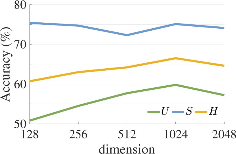
(a) AWA

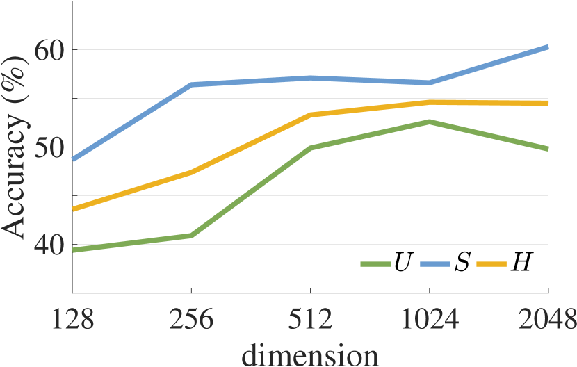
(b) CUB

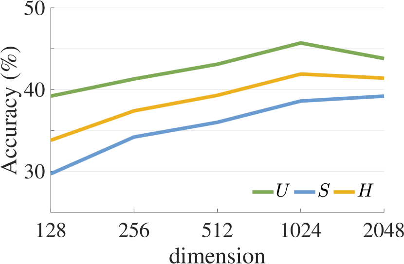
(c) SUN

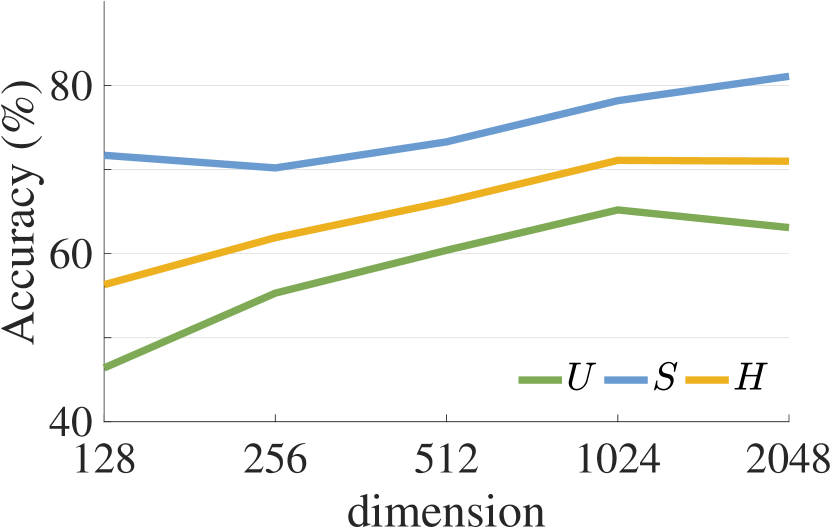
(d) FLO

Figure 5: The influence of the redundancy-free feature dimensions on GZSL results, evaluated by our RFF-GZSL.

We first compare our redundancy-free feature generation results with the other feature generation methods. Our RFF-GZSL is competitive compared with the feature generation methods. Specifically, according to the harmonic mean results, our RFF-GZSL can surpass the eight feature generation methods on AWA, SUN and FLO. On CUB, our RFF-GZSL is only lower than GMN [47] and SABR [43]. And on FLO, our method outperform the second best method by a large margin. Then, we compare our RFF-GZSL with the non-feature generation methods. Our method can achieve the best results evaluated on the unseen classes ($U$) and the harmonic mean ($H$) on CUB and SUN. And our method achieves the second best on $U$ and $S$ on AWA. The results demonstrates the effectiveness of our RFF-GZSL.

In Figure 4, we report our RFF-GZSL results under different numbers of synthesized samples per unseen class. When the amount of synthetic samples is small, the $U$ and $H$ results are low due to the data imbalance problem. As the number of synthetic features increases, the $U$ and $H$ results improve significantly, which means our redundancy-free feature generation method can deal with the data imbalance problem in GZSL.

We also evaluate our feature generation method, RFF-GZSL, with different dimensions of redundancy-free feature space, as shown in Figure 5. When the dimension is small, our performances on four datasets are low. As the dimension increases, the performances on these four datasets get better. With the dimension of the redundancy-free feature space equal to 1,024, we can already achieve the satisfactory GZSL results on the four datasets.

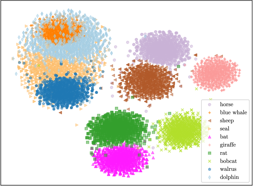
(a) f-CLSWGAN

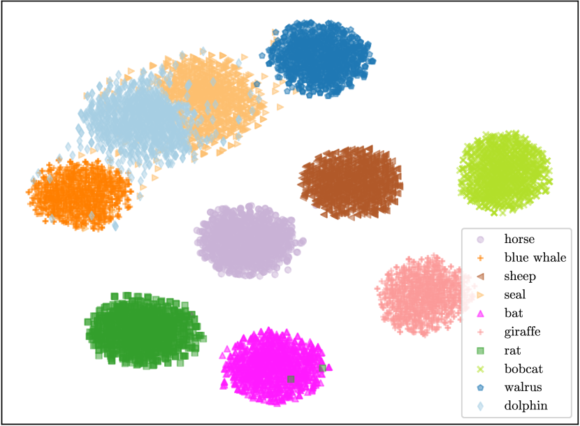
(b) Our RFF-GZSL

Figure 6: Visualization of the synthetic feature distributions of f-CLSWGAN [53] and our RFF-GZSL on AWA.

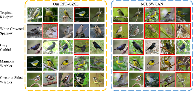
Figure 7: The results of image retrieval. Each row contains the Top-5 retrieved images of a specific class. The image with a red box means a wrong retrieval.

4.2 Comparison with traditional ZSL methods

In this section, we compare the redundancy-free semantic embedding model with several traditional ZSL methods in the new generalized ZSL scenario. Table 2 shows the compared results. It can be seen that the traditional ZSL methods usually perform poor in the GZSL setting. Especially, all traditional ZSL methods in Table 2 can achieve a high performance ($S$) on the seen classes, but perform poor ($U$) on the unseen classes, resulting in a low harmonic mean ($H$) for GZSL. Our redundancy-free semantic embedding model can enhance the performance of the traditional semantic embedding methods by reducing the redundancy information in the original visual features. Specifically, our method is built upon SJE [2]; compared with SJE [2], our redundancy-free semantic embedding method can improve the GZSL results significantly on AWA and FLO with almost 15% enhancement. Finally, our method can surpass all compared traditional ZSL methods on the new GZSL task.

4.3 Visualization Results

Feature visualization

We visualize the features used in the final GZSL classification with t-SNE [32]. We compare the visualization result of our redundancy-free feature generation with f-CLSWGAN [53] on AWA to investigate the structure of generated features. Concretely, for each unseen class on AWA, we use the learned composite feature generator in our method to synthesize 1,000 features in the redundancy-free feature space, while we apply f-CLSWGAN to synthesize 1,000 features in the original visual feature space. Since the dimension of the visual feature space is 2,048, for a fair comparison, we let our redundancy-free feature space have the same dimension. The results of f-CLSWGAN and ours are shown in Figure 6(a) and Figure 6(b), respectively. As shown in Figure 6(a), in the generated visual feature space of f-CLSWGAN, the feature distributions of four animal categories, i.e. blue whale, seal, walrus and dolphin, are highly overlapping. After reducing the redundancy information from the visual features, as shown in 6(b), these four and other unseen categories can be easily separated in our redundancy-free feature space.

Image Retrieval

We compare our RFF-GZSL with f-CLSWGAN [53] on the image retrieval task on CUB. Specifically, we use our RFF-GZSL to synthesize 10 features in the redundancy-free feature space for each unseen CUB class and then we apply the mean of these 10 features to query the top-5 images, which have been mapped in the same redundancy-free feature space. We do the same thing using f-CLSWGAN [53], but this time the synthetic features locating in the original visual feature space. Figure 7 shows the top-5 retrieval results of five bird example categories. The retrieval results of our method are more accurate than f-CLSWGAN, demonstrating that the learned redundancy-free features in our method are more discriminative than the original visual features.

5 Conclusion

In this work, we have proposed to learn the redundancy-free features for generalized zero-shot object recognition. We accomplish it by learning a mapping function to map the original visual features to a new redundancy-free feature space. We bound the statistical dependence between these two feature spaces to remove the redundant information from the visual features. Our method can integrate with existing GZSL frameworks. The performance of conventional semantic embedding methods has been promoted significantly using the redundancy-free features. Our redundancy-free feature generation model can achieve the state-of-the-art or competitive results on four benchmarks. Also, the visualization results, including the feature distribution and the image retrieval, further demonstrate the effectiveness of learning the redundancy-free features for GZSL.

References

- [1] Zeynep Akata, Florent Perronnin, Zaid Harchaoui, and Cordelia Schmid. Label-embedding for attribute-based classification. In CVPR, 2013.
- [2] Zeynep Akata, Scott Reed, Daniel Walter, Honglak Lee, and Bernt Schiele. Evaluation of output embeddings for fine-grained image classification. In CVPR, 2015.
- [3] Alexander A Alemi, Ian Fischer, Joshua V Dillon, and Kevin Murphy. Deep variational information bottleneck. arXiv preprint arXiv:1612.00410, 2016.
- [4] Martin Arjovsky, Soumith Chintala, and Léon Bottou. Wasserstein gan. arXiv preprint arXiv:1701.07875, 2017.
- [5] Yuval Atzmon and Gal Chechik. Adaptive confidence smoothing for generalized zero-shot learning. In CVPR, 2019.
- [6] Yoshua Bengio, Li Yao, Guillaume Alain, and Pascal Vincent. Generalized denoising auto-encoders as generative models. In NIPS, 2013.
- [7] Maxime Bucher, Stéphane Herbin, and Frédéric Jurie. Improving semantic embedding consistency by metric learning for zero-shot classiffication. In European Conference on Computer Vision, 2016.
- [8] Maxime Bucher, Stéphane Herbin, and Frédéric Jurie. Generating visual representations for zero-shot classification. In ICCV, 2017.
- [9] Soravit Changpinyo, Wei-Lun Chao, Boqing Gong, and Fei Sha. Synthesized classifiers for zero-shot learning. In CVPR, 2016.
- [10] Long Chen, Hanwang Zhang, Jun Xiao, Wei Liu, and Shih-Fu Chang. Zero-shot visual recognition using semantics-preserving adversarial embedding networks. In CVPR, 2018.
- [11] Ali Farhadi, Ian Endres, Derek Hoiem, and David Forsyth. Describing objects by their attributes. In CVPR, 2009.
- [12] Rafael Felix, Vijay BG Kumar, Ian Reid, and Gustavo Carneiro. Multi-modal cycle-consistent generalized zero-shot learning. In ECCV, 2018.
- [13] Andrea Frome, Greg S Corrado, Jon Shlens, Samy Bengio, Jeff Dean, Tomas Mikolov, et al. Devise: A deep visual-semantic embedding model. In NIPS, 2013.
- [14] Zhenyong Fu, Tao Xiang, Elyor Kodirov, and Shaogang Gong. Zero-shot object recognition by semantic manifold distance. In CVPR, 2015.
- [15] Zhenyong Fu, Tao Xiang, Elyor Kodirov, and Shaogang Gong. Zero-shot learning on semantic class prototype graph. TPAMI, 2017.
- [16] Ian Goodfellow, Jean Pouget-Abadie, Mehdi Mirza, Bing Xu, David Warde-Farley, Sherjil Ozair, Aaron Courville, and Yoshua Bengio. Generative adversarial nets. In NIPS, 2014.
- [17] Ishaan Gulrajani, Faruk Ahmed, Martin Arjovsky, Vincent Dumoulin, and Aaron C Courville. Improved training of wasserstein gans. In NIPS, 2017.
- [18] Kaiming He, Xiangyu Zhang, Shaoqing Ren, and Jian Sun. Deep residual learning for image recognition. In CVPR, 2016.
- [19] He Huang, Changhu Wang, Philip S Yu, and Chang-Dong Wang. Generative dual adversarial network for generalized zero-shot learning. In CVPR, 2019.
- [20] Diederik P Kingma and Jimmy Ba. Adam: A method for stochastic optimization. arXiv preprint arXiv:1412.6980, 2014.
- [21] Diederik P Kingma and Max Welling. Auto-encoding variational bayes. arXiv preprint arXiv:1312.6114, 2013.
- [22] Elyor Kodirov, Tao Xiang, Zhenyong Fu, and Shaogang Gong. Unsupervised domain adaptation for zero-shot learning. In ICCV, pages 2452--2460, 2015.
- [23] Elyor Kodirov, Tao Xiang, and Shaogang Gong. Semantic autoencoder for zero-shot learning. In CVPR, 2017.
- [24] Alex Krizhevsky, Ilya Sutskever, and Geoffrey E Hinton. Imagenet classification with deep convolutional neural networks. In NIPS, 2012.
- [25] Vinay Kumar Verma, Gundeep Arora, Ashish Mishra, and Piyush Rai. Generalized zero-shot learning via synthesized examples. In CVPR, 2018.
- [26] Christoph H Lampert, Hannes Nickisch, and Stefan Harmeling. Learning to detect unseen object classes by between-class attribute transfer. In CVPR, 2009.
- [27] Christoph H Lampert, Hannes Nickisch, and Stefan Harmeling. Attribute-based classification for zero-shot visual object categorization. TPAMI, 2014.
- [28] Jingjing Li, Mengmeng Jing, Ke Lu, Zhengming Ding, Lei Zhu, and Zi Huang. Leveraging the invariant side of generative zero-shot learning. In CVPR, 2019.
- [29] Kai Li, Martin Renqiang Min, and Yun Fu. Rethinking zero-shot learning: A conditional visual classification perspective. In ICCV, 2019.
- [30] Yujia Li, Kevin Swersky, and Rich Zemel. Generative moment matching networks. In ICML, 2015.
- [31] Shichen Liu, Mingsheng Long, Jianmin Wang, and Michael I Jordan. Generalized zero-shot learning with deep calibration network. In NeurIPS, 2018.
- [32] Laurens van der Maaten and Geoffrey Hinton. Visualizing data using t-sne. JMLR, 2008.
- [33] Alireza Makhzani, Jonathon Shlens, Navdeep Jaitly, Ian Goodfellow, and Brendan Frey. Adversarial autoencoders. arXiv preprint arXiv:1511.05644, 2015.
- [34] Tomas Mikolov, Kai Chen, Greg Corrado, and Jeffrey Dean. Efficient estimation of word representations in vector space. arXiv preprint arXiv:1301.3781, 2013.
- [35] Tomas Mikolov, Ilya Sutskever, Kai Chen, Greg S Corrado, and Jeff Dean. Distributed representations of words and phrases and their compositionality. In NIPS, 2013.
- [36] Ashish Mishra, Shiva Krishna Reddy, Anurag Mittal, and Hema A Murthy. A generative model for zero shot learning using conditional variational autoencoders. In CVPR, 2018.
- [37] Maria-Elena Nilsback and Andrew Zisserman. Automated flower classification over a large number of classes. In ICCVGI, 2008.
- [38] Mohammad Norouzi, Tomas Mikolov, Samy Bengio, Yoram Singer, Jonathon Shlens, Andrea Frome, Greg S Corrado, and Jeffrey Dean. Zero-shot learning by convex combination of semantic embeddings. arXiv preprint arXiv:1312.5650, 2013.
- [39] Augustus Odena, Christopher Olah, and Jonathon Shlens. Conditional image synthesis with auxiliary classifier gans. In ICML, 2017.
- [40] Mark Palatucci, Dean Pomerleau, Geoffrey E Hinton, and Tom M Mitchell. Zero-shot learning with semantic output codes. In NIPS, 2009.
- [41] Devi Parikh and Kristen Grauman. Relative attributes. In ICCV, 2011.
- [42] Genevieve Patterson and James Hays. Sun attribute database: Discovering, annotating, and recognizing scene attributes. In CVPR, 2012.
- [43] Akanksha Paul, Narayanan C Krishnan, and Prateek Munjal. Semantically aligned bias reducing zero shot learning. In CVPR, 2019.
- [44] Xue Bin Peng, Angjoo Kanazawa, Sam Toyer, Pieter Abbeel, and Sergey Levine. Variational discriminator bottleneck: Improving imitation learning, inverse RL, and GANs by constraining information flow. In ICLR, 2019.
- [45] Scott Reed, Zeynep Akata, Honglak Lee, and Bernt Schiele. Learning deep representations of fine-grained visual descriptions. In CVPR, 2016.
- [46] Bernardino Romera-Paredes and Philip Torr. An embarrassingly simple approach to zero-shot learning. In ICML, 2015.
- [47] Mert Bulent Sariyildiz and Ramazan Gokberk Cinbis. Gradient matching generative networks for zero-shot learning. In CVPR, 2019.
- [48] Edgar Schonfeld, Sayna Ebrahimi, Samarth Sinha, Trevor Darrell, and Zeynep Akata. Generalized zero-and few-shot learning via aligned variational autoencoders. In CVPR, 2019.
- [49] Richard Socher, Milind Ganjoo, Christopher D Manning, and Andrew Ng. Zero-shot learning through cross-modal transfer. In NIPS, 2013.
- [50] Catherine Wah, Steve Branson, Peter Welinder, Pietro Perona, and Serge Belongie. The caltech-ucsd birds-200-2011 dataset. 2011.
- [51] Yandong Wen, Kaipeng Zhang, Zhifeng Li, and Yu Qiao. A discriminative feature learning approach for deep face recognition. In ECCV, 2016.
- [52] Yongqin Xian, Zeynep Akata, Gaurav Sharma, Quynh Nguyen, Matthias Hein, and Bernt Schiele. Latent embeddings for zero-shot classification. In CVPR, 2016.
- [53] Yongqin Xian, Tobias Lorenz, Bernt Schiele, and Zeynep Akata. Feature generating networks for zero-shot learning. In CVPR, 2018.
- [54] Yongqin Xian, Bernt Schiele, and Zeynep Akata. Zero-shot learning-the good, the bad and the ugly. In CVPR, 2017.
- [55] Yongqin Xian, Saurabh Sharma, Bernt Schiele, and Zeynep Akata. f-vaegan-d2: A feature generating framework for any-shot learning. In CVPR, 2019.
- [56] Guo-Sen Xie, Li Liu, Xiaobo Jin, Fan Zhu, Zheng Zhang, Jie Qin, Yazhou Yao, and Ling Shao. Attentive region embedding network for zero-shot learning. In CVPR, 2019.
- [57] Fei Zhang and Guangming Shi. Co-representation network for generalized zero-shot learning. In ICML, 2019.
- [58] Ziming Zhang and Venkatesh Saligrama. Zero-shot learning via semantic similarity embedding. In CVPR, 2015.
- [59] Jun-Yan Zhu, Taesung Park, Phillip Isola, and Alexei A Efros. Unpaired image-to-image translation using cycle-consistent adversarial networks. In ICCV, 2017.