Improving the Performance of Deep Learning
for Wireless Localization

Abstract

Indoor localization systems are most commonly based on Received Signal Strength Indicator (RSSI) measurements of either WiFi or Bluetooth-Low-Energy (BLE) beacons. In such systems, the two most common techniques are trilateration and fingerprinting, with the latter providing higher accuracy. In the fingerprinting technique, Deep Learning (DL) algorithms are often used to predict the location of the receiver based on the RSSI measurements of multiple beacons received at the receiver.

In this paper, we address two practical issues with applying Deep Learning to wireless localization — transfer of solution from one wireless environment to another and small size of labelled data set. First, we apply automatic hyperparameter optimization to a deep neural network (DNN) system for indoor wireless localization, which makes the system easy to port to new wireless environments. Second, we show how to augment a typically small labelled data set using the unlabelled data set. We observed improved performance in DL by applying the two techniques. Additionally, all relevant code has been made freely available.

I Introduction

Systems like GPS have made outdoor localization very prevalent. However, in an indoor setting, GPS does not work and other approaches have to be taken to perform localization. Indoor localization has a lot of uses such as device and personnel tracking, targeted advertising, and broadcasting localized information.

One of the most common ways of performing indoor localization is to use the reception of wireless signals at any wireless receiver, such a laptop or mobile handset. In particular, the Received Signal Strength Indicator (RSSI) at any receiver has a correlation with the location of the source of the signal. The two most common ways of using RSSI measurements to predict the location of the receiver are trilateration (sometimes called triangulation) and fingerprinting. Trilateration [1] is the process of using the estimated distances from multiple sources to triangulate a most probable location of the receiver. The earliest works in localization have used this approach [2]. Obviously, the radio frequency propagation of the environment has a great impact on the accuracy of this method. For example, effects like multi-path can cause a lot of noise in the received signal.

Fingerprinting [3] on the other hand is somewhat more resilient to the idiosyncrasies of the environment because it relies on prior measurements being collected for multiple known locations in a specific environment – one fingerprint for each measured location, so to say. This takes care of any vagaries of the environment affecting the path loss propagation model. Of course any drastic change in the environment will make the measurements less relevant. Once the measurements are collected, the system then predicts the location of the receiver by comparing the RSSI measurements with the fingerprints for different locations and selecting the one with the most similar fingerprint as the most probable location of the receiver.

Due to the prevalence of IEEE 802.11-WiFi deployments, the initial fingerprinting based systems used the RSSI measurements of WiFi beacons. However, Bluetooth Low Energy (BLE) is fast becoming an alternate to WiFi access points since BLE transmitters consume much less energy compared to WiFi access points. This allows BLE transmitters to run on battery for months and even years and hence can be installed without any worry of access to power. Additionally, the BLE approach seems to be able to provide more fine grained localization than WiFi based solutions, as reported by Zhao et al. [4, 5, 6]. The reasons behind why BLE outperforms WiFi for localization is outside the scope of this paper.

I-A Issues with Deep Learning in Wireless Localization

There are several ML algorithms that are used in the fingerprinting approach. Some of these are $k$-nearest neighbors, support vector machines, probabilistic methods (e.g., Naive Bayes), and deep neural networks (DNN) – a good survey is presented by Liu et al. [1] and Bozkurt et al. [7]. However, using ML, specifically DNNs, for this has several issues and in this paper, we address the following two major issues.

First, each layout/floor map would need a different model or one may use the same model architecture and tune it for each layout. Even without any change in the layout, since wireless environment is dynamic due to multi-path effect, noise, etc., frequent tuning of the models is a necessity. Automatic tuning of the model gives us a quick, scalable way of tuning, thus improving models. A typical problem in using DNNs (used in any problem domain and not just RSSI fingerprinting) is that these neural networks usually have quite a few hyperparameters (knobs), such as learning rate, number of hidden nodes, and batch size, that have to be set before the training process. These knobs generally have a large impact on the metrics of the neural network, such as training time and accuracy and hence tuning these knobs is essential to improve the performance of the neural network. Consequently, figuring out the optimum values for these knobs (hyperparameters) is non-trivial. So, automatic hyperparameter tuning (HP-tuning) is important for finding a better model for any given layout. In this paper, we show how hyperparameter optimization can be applied to a DNN (that would otherwise have to be manually tuned) to perform RSSI fingerprint matching.

Second, a typical problem in data collection for wireless localization is that number of labelled data points is largely outnumbered by the number of unlabelled data points. Due to this lack of labelled data, the ML algorithms trained on the data are difficult to generalize, thus making the learning less transferable to other wireless environments. In this work, we present augmentation techniques for augmenting the unlabelled samples.

I-B Related Work

As mentioned in Section I, there have been several pieces of work in using ML in the area of fingerprint based indoor localization [1]. There has also been work on using principal component analysis (PCA) to reduce computation cost of ML-based WiFi indoor localization [8]. Here we explain some deep learning based work that are relevant to our work. Zhang et al. [9] addressed important issues with deep neural networks for both indoor and outdoor wireless localization. However, they did not analyze the use of HP-tuning or augmentation of the data set. To the best of our knowledge we could not find any prior work related to the application of hyperparameter tuning (HP-tuning) to DNNs for wireless localization. Similarly, there are augmentation techniques available for image related machine learning models [10] but we could not find anything related to augmentation of wireless RSSI samples.

One of the problems in working with existing DNN models for wireless localization is that the code for the models are often not publicly available making it difficult to analyze and extend the work. In this respect, Kaggle [11] is a widely used source of publicly available models making it easy to analyze the code, fix any issues, and contribute back extensions or corrections to the models; we chose this path to get a DNN from Kaggle[12]. We also introduced a CNN model of our own. We used these as the base code to perform HP-tuning.

I-C Our Contributions

This paper addresses the issue mentioned above and our main contributions can be summarized as follows:

• We present the design and analysis of applying HP-tuning to a deep neural network (DNN) system for indoor wireless localization.

• We introduce a convolutional neural network (CNN) model for wireless localization and apply HP-tuning to it as well.

• We present an augmentation technique to augment the labelled data sets with data points from the unlabelled data set.

• We have also made all relevant code public so that our work can be easily verified and extended.

The rest of this paper is arranged as follows. Section II gives an overview of hyperparameter optimization. We explain the data set used in this paper in Section III. In Section IV, we give an overview of our implementation setup used to run all our experiments. Section V explains the DNN and CNN models and the impact of applying HP-tuning to them. We present how the labelled data set can be augmented using data points from the unlabelled data set in Section VI. Finally, we conclude in Section VII.

II Background: Hyperparameter Optimization

In machine learning, a hyperparameter is a parameter that must be fixed before the actual training process. Consequently, hyper-parameters (e.g., learning rate, batch size, and number of hidden nodes) cannot be learnt during the learning process, unlike the value of parameters (e.g., weights) that are learned during the training process. Hyperparameters can impact both the quality of the model generated by the training process as well as the time and memory requirements of the algorithm [13]. Thus, hyperparameters have to be tuned to get the optimal setting for a given problem. This tuning can be done either manually or automatically. Manual tuning might suffice if the problem setup is not expected to change, at least not frequently. In case the problem setup is expected to change frequently, an automatic hyperparameter tuning (HP-tuning) mechanism is required to make the system practical.

There are several common algorithms that are used in automatic hyperparameter tuning. Some of the most common are:

• Grid search: Given a range of possible values for each of the hyperparameters, this exhaustive algorithm runs experiments with all hyperparameter values in the Cartesian product of the set of values for each individual hyperparameter. This technique works best when there are few hyperparameters ($<=3$).

• Random search: This improves upon the grid search method by searching the range of each hyperparameter randomly rather than exhaustively. This leads to faster search times and hence works better than grid search, especially when the number of hyperparameters is large.

• Bayesian optimization: In contrast to grid or random search, Bayesian optimization uses a probability model of the objective function and uses that to select the most promising hyperparameter values [14]. We use this search technique in this paper.

Figure 1: The experimental setup with 13 iBeacons in a $200ft.$ X $180ft.$ library [15, 16].

III Data Set

Our evaluation is based on a real world data set that is available at the Machine Learning Repository, made public by the University of California, Irvine [15]. This data set was first presented by Mohammadi et al. [16] and much of the description of the data set presented here has been taken from the original paper.

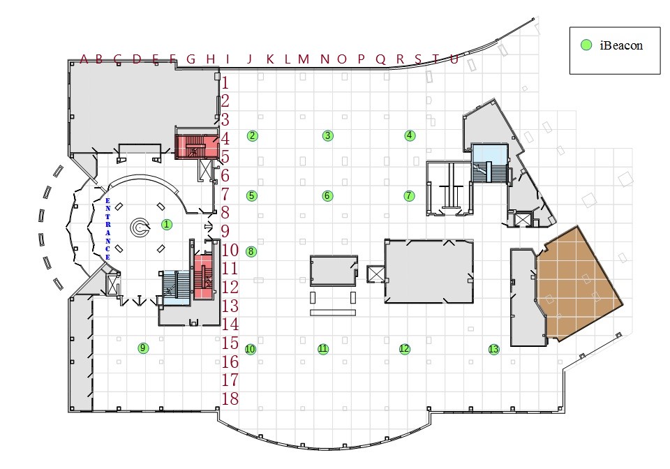
The data set is from a real-world deployment of 13 of Apple’s iBeacons, which use the Bluetooth Low Energy (BLE) standard of Bluetooth 4.0, in a campus library of dimension 200 ft. X 180 ft. These beacons are installed on the ceiling of the first floor of the Waldo Library in Western Michigan University, USA. On an average, each of the 13 iBeacons are at a distance of around 30-40 ft. from nearby iBeacons. The entire floor space was divided in 10 ft. X 10 ft. block and the RSSI measurements were taken at several locations, with each location being manually captured. Each location is usually covered by multiple beacons and all those measurements were captured. The entire labelled data set contains 1136 data points used for training and 284 data points for testing, which is a typical 80:20 split of the total 1420 labelled data points. In addition to the labelled samples, there are 5191 unlabelled samples as well. As mentioned in Section I, this is a typical problem in sample collection and we will address this issue in Section VI.

Setup/Parameter	Value
Hyperparameter Tuner	Katib
ML framework	Keras
Epochs	100
Batch Size	100
Activation Function	ReLU
Loss Function	Root mean squared error (rmse)
Optimizer	Adam, SGD
Number of parameters	DNN: 6102, CNN: 5438
Training data points	1136
Test data points	284

TABLE I: Training Setup and Parameters. A single forward and backward pass of the entire data set through the neural network is defined as an epoch. Since entire data set might be too large to train in one shot, the data set is divided into batch size chunks.

IV Implementation Details

This section describes the implementation details for the rest of the paper. We provisioned a Kubernetes [17] cluster, and deployed Katib (Appendix -A), the open source hyperparameter tuner, on Kubeflow (Appendix -B), the ML toolkit for Kubernetes. We implemented all the ML models in Keras [18]. We packaged each Keras model, which takes hyperparameters as input and emits loss metric as the output, into a Docker [19] image. These images are used in Katib user interface trial specification to trigger the trials. The range of hyperparameters is set accordingly for each optimizer in the user interface, e.g., for Adam optimizer, learning rate – [0.001, 0.002], beta1 – [0.88, 0.93]. The objective metric to be minimized is set to Euclidean/l2 loss, with a goal of 1.2, specified in the user interface. Also, we limited the maximum trials for each tuning experiment to 15 and chose the Bayesian optimization algorithm. All code relevant to this paper has been made public at https://github.com/CiscoAI/deep-learning-wireless-localization.

V DNN and CNN for Wireless Localization

As mentioned earlier, deep neural networks have been used since quite sometime to address wireless localization, especially using the fingerprinting technique.

V-A DNN

Figure 2: DNN Architecture. $[$Input layer: 13 nodes, 1 each for each iBeacon; Hidden layers: 3 layers, each with 50 nodes; Output layer: 2 nodes, representing (x,y) coordinates of predicted location; Activation function: ReLU$]$

(a) Adam Optimizer DNN.

(b) SGD Optmizer in DNN.

Figure 3: Hyperparameter optimization using Bayesian optimization applied to DNN. The arrows mark the optimal values.

Figure 4: The CNN architecture. $[$Input layer: [25, 25, 1] grayscale image; 2 Convolution layers: number of filters respectively [12, 12]; Filter sizes: [7, 7], [5, 5] with valid padding; 1 Dense layer: 24 nodes; Output layer: 2 representing $x$ and $y$ coordinates; Activation function: ReLU$]$

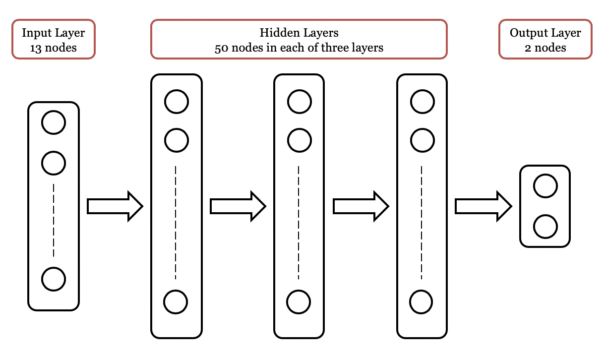
A deep neural network (DNN) is any neural network that has layers in addition to the input and output layers; these additional layers are known as hidden layers. The number of hidden layers can vary from a few (2–3) to thousands. For our study we used an existing DNN model [12], shown here in Figure 2. The DNN takes in each of the 13 RSSI measurements and tries to predict the $<$x,y$>$ coordinates of the location where the measurement was made. The data set described in Section III was used with a 80:20 (1136:284) train:test split. The training parameters are specified in Table I.

V-B DNN with Hyperparameter Optimization

Sl. No	Setup	default learning rate	tuned learning rate	default beta1	tuned beta1	default momentum	tuned momentum	loss metric with default	loss metric with tuned parameters
1.	DNN + Adam	0.001	0.00197	0.9	0.89177	—	—	2.32	2.2
2.	DNN + SGD	0.01	0.015	—	—	0.9	0.905	2.10	1.97
3.	CNN + Adam	0.001	0.00177	0.9	0.885	—	—	2.4	2.11
4.	CNN + SGD	0.01	0.01375	—	—	0.9	0.885	2.36	2.10

TABLE II: Hyperparameter values and loss metrics. Loss metrics are in units of grid length, i.e., 2.2 means 2.2 x 10ft = 22 ft.

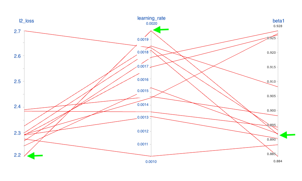
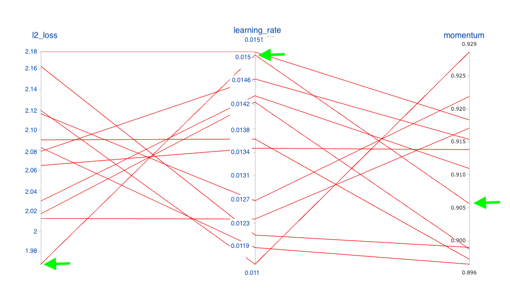
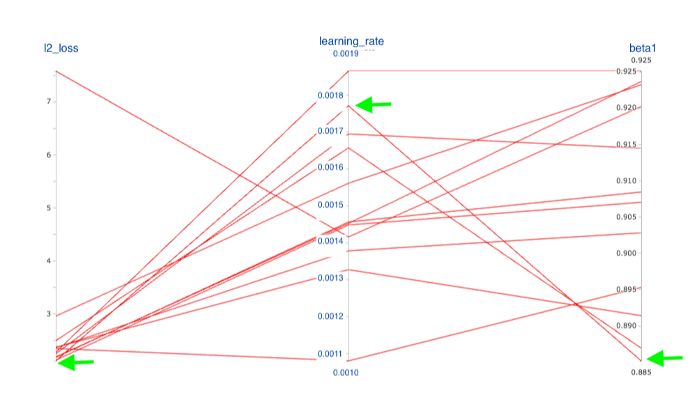
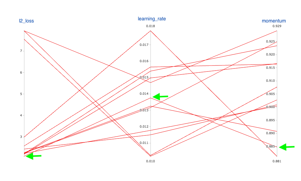
As explained earlier, the performance of a model is affected by the choice of the hyperparameters and figuring out the optimal value for of the hyperparameters is non-trivial. This issue is magnified if the underlying wireless environment changes. Consequently, we apply hyperparameter tuning (HP-tuning) to the DNN and check if it provides any advantage. The result of the experiment are shown in Figure 3. The HP-tuning was tried for both the Adam optimizer [20] and the Stochastic Gradient Descent (SGD) optimizer [21] and the results are shown respectively in Figure 3(a) and Figure 3(b). For the Adam optimizer, the hyperparameters are the learning rate, beta1, and beta2 and for the SGD the hyperparameters are learning rate and momentum. In order to make both graphs comparable, we just used beta1 and left out beta2. The figures show how the different values of the hyperparameters impact the metric, the l2 loss. From Figure 3 the following can be observed (as consolidated in Table II):

• The best combination for the Adam optimizer (Figure 3(a)) is a learning rate value of 0.002 and beta1 value of 0.893. This gives an l2 loss of 22 feet.

• The best combination for the SGD optimizer (Figure 3(b)) is an learning rate value of 0.015 and momentum value of 0.905. This gives and l2 loss of 19.7 feet.

• Even a small change in the value of learning rate can significantly impact the metric.

• The l2 loss varies from 22.0ft to 27.0ft for the Adam optimizer (Figure 3(a)) and from 19.6ft to 21.8ft for the SGD optimizer (Figure 3(b)). This means that the SGD optimizer is a better optimizer for this problem compared to the Adam optimizer.

Apart from learning rate, other hyperparameters such as batch size, number of layers, and layer sizes can also be tuned using the tuning framework, thus allowing an optimal search of the entire search space to find the best set of hyperparameters. However, we did not perform this exhaustive search for this paper.

V-C CNN

A DNN has a major disadvantage that the model is tied to the number of beacons – if there is a change in the number of beacons, the model has to be reconstructed since the same model might not work for scenarios with a large difference in the number of beacons. In order to handle this, a special type of DNN, called a Convolutional Neural Network (CNN) can be used. CNNs are neural networks that use convolutions, a special kind of linear operation, as opposed to the typical matrix multiplication, in at least one of the layers of the neural network. CNNs are most useful when the data being processed has a grid like topology such as, most commonly, image data, but also time series data [13].

(a) Adam Optimizer in CNN

(b) SGD Optmizer in CNN

Figure 5: Hyperparameter optimization using Bayesian optimization applied to CNN. The arrows mark the optimal values.

Figure 6: Comparison of CNN and DNN with and without hyperparameter (HP) optimization with the Adam optimizer. A steeper and higher curve is better.

We took a CNN model available on Kaggle [12] and made obvious changes to improve model performance. We changed the filter sizes, increased the number of feature maps, and replaced last CNN layer with a dense layer; Figure 4 shows the architecture. The epochs, batch size, loss function, train:test split, are the same as specified in Table I. In order to apply CNN to the problem of wireless localization, the data is converted into a gray scale image. Each of the data instance (i.e., a row of 13 iBeacons RSSI values corresponding to a specific location) is transformed into a gray scale image of size [25,25,1], corresponding to 25 X 25 grids in which the entire floor map (Figure 1) is divided into. Thus, there as many images as there are samples in the data set. The image is created via the following steps:

1. The image is initialized to a zeroed image of size [25, 25, 1], i.e., an image with just black pixels.

2. Each beacon’s sensor location coordinates (x,y,1) is assigned with a pixel value that is obtained by dividing the RSSI measurement by -200 (minimum RSSI value). This normalizes the pixel values to the [0,1] range.

As an example, suppose a receiver located at $<$10, 15$>$ measures an RSSI of $-20$ dBm for iBeacon $i$, which has a location of $<x_{i},y_{i}>$, then the value of coordinate $<x_{i},y_{i},1>$ is set to the normalized value of $-20/-200$ dBm. This sample image is then labelled with the $<x,y>$ coordinates of the receiver, $<$10, 15$>$. Such an image is generated for each location of the receiver thus making as many images as there are samples in the data set. The CNN is then trained such that given a gray scale image, the neural network predicts the corresponding $x$ and $y$ coordinates of the receiver.

(a) Overall distribution of 1420 samples.

(b) 188 under-represented ($<10$ samples) locations in the data set.

Figure 7: Distribution of labelled samples in the data set. The $z$-axis shows the number of samples for the corresponding grid (25 X 25) specified by the $x$ and $y$ axes.

Figure 8: Autoencoder architecture for data augmentation.

Figure 9: Location Prediction Error with Augmentation for a DNN model with Adam optimizer and default hyperparameters. The naive and standard autoencoder based augmentations improve the performance compared to the original data set. The hybrid approach shows the most improvement.

V-D CNN with Hyperparameter Optimization

Just like in the case of DNN, we apply HP-tuning using Bayesian optimization to the CNN and the results are shown in Figure 5. Overall the pattern looks similar to using hyperparameter optimization with DNN (Figure 3) but the main difference to note is that the range of the metric values (l2 loss) is much higher in the case of CNN than in the case of DNN, with both the Adam and the SGD optimizer. This means that hyperparameter search is more relevant with the use of CNN than DNN when applied to the wireless localization problem.

V-E CNN and DNN Comparison

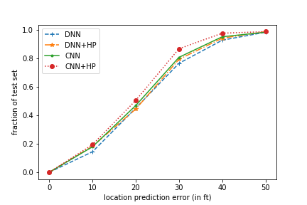
Figure 6 shows the comparison of the different models, all with Adam optimizer. The Y-axis shows the fraction of test samples that were predicted within a prediction error, shown in the X-axis. All the models perform very similar though there is noticeable difference between them. As expected the base DNN model performs the worst and DNN with HP-tuning does improve the performance marginally. This is expected from row 1 of Table II that shows that the tuned learning rate and beta1 are very close to their respective default values. As the number of beacons increases, we expect that HP-tuning for DNNs would yield further gains. The base CNN model shows performance very close to the DNN with HP-tuning but the CNN with HP-tuning does show a noticeable improvement.

The exact DNN or CNN model is not that relevant here. The most important thing that we want to convey is that hyperparameter tuning allows a quick and automatic search to find the best hyperparameters for any given model.

VI Dataset Augmentation

A basic problem with location samples is that compared to the total number of samples, only a small fraction are labelled. For example, as mentioned earlier in Section III, in the BLE data set [15], there are only 1420 labelled samples but a much larger 5191 unlabelled samples. In general, ML models perform better with larger training samples.

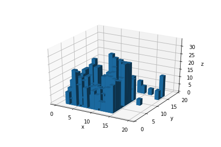
We started by analysing the distribution of samples with respect to the grid (Figure 1). As shown in Figure 7(a), different grids have different number of samples and the distribution is not uniform. This is expected since the library floor has pillars and furniture that makes several grid locations inaccessible. On top of it since the data collection is done by humans it is simply unrealistic to expect equal number of samples at each location. We need to augment these under-represented areas (Figure 7(b)) for better prediction in these areas.

VI-A Naive Approach

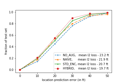
We first tried a naive approach to augment the data set. This approach does not use any unlabelled sample. In this approach, for a location with fewer samples ($<10$), as shown in Figure 7(b), new samples (with the same label, i.e., the same location) are generated using a uniform distribution between the minimum and maximum value of the RSSI for any given beacon. For example, if a location has two samples, one with RSSI values from beacons b1, b2, and b3, and the other from just b1 and b2, a new sample is generated with RSSI values for b1 and b2 as a random sample between the minimum and maximum RSSI values from the two respective samples; b3 is skipped since it is not present in both the samples and hence the minimum and maximum of the RSSI values for b3 are undefined. We use this to generate one additional sample for each of the 188 under-represented locations. With this approach we were able to generate another 188 labelled sample points thus giving a total of 1420 + 188 = 1608 labelled samples that we used for training and testing. The results with this augmented data set for a DNN with Adam optimizer and default hyperparameters are shown in Figure 9 and the naive approach shows a distinct advantage over the original data set; mean error reduces from 23.2 ft to 21.9 ft. However, as already mentioned, this approach does not utilize the unlabelled samples; we address that issue with the use of autoencoders.

VI-B Standard Autoencoder

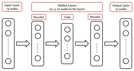
Autoencoders are a standard technique for augmenting data sets and we wanted to check whether it can be used for our data set. Goodfellow et al. [13] define an autoencoder as a neural network that is trained to attempt to copy its input to its output. As shown in Figure 8, it has an input layer and an output layer that is separated by one ore more hidden layers. The hidden layers constitute an encoder that encodes the input into a lower dimension code and a decoder that tries to reconstruct the original image from the code. A more detailed description of autoencoders is outside the scope of this paper.

The autoencoder is run for 20 epochs, with each epoch processing the entire set of 5191 unlabelled images. Thus the autoencoder learns the distribution of the unlabelled data set. Once this is done, we take one sample for each of the 188 under-represented locations and feed it to the autoencoder and use the output as an additional sample, with the same label as the input sample. Though 188 samples were fed, there were some samples generated that were showing RSSI values for beacons that the location had not seen in any of the existing samples. There were 30 such generated samples and these were discarded. This left us with 188 - 30 = 158 samples and the labelled data set was augmented to 1420 + 158 = 1578 samples. Figure 9 shows that the 20.7 ft mean error with this augmented data is slightly better than the 21.9 ft mean error with the naive approach.

The natural thing to do is to combine both the previous approaches into a hybrid approach. This gives an additional 188 + 158 samples, thus taking the overall count of labelled samples to 1420 + (188 + 158) = 1766. As expected, and as shown in Figure 9, this hybrid approach gives the best performance with a mean error of 19.7 ft. Overall, this amounts to around 15% reduction in the prediction error. In this work, we created just one additional sample for each under-represented location, if needed, more samples for these locations can be generated.

VII Conclusion

In this paper, we have presented two techniques for improving the performance of deep learning models for wireless localization. First, we analysed how hyperparameter optimization can be applied to DNN and CNN models to optimize their performance and to make them more relevant to wireless environments, which are naturally very dynamic. Second, we present two augmentation techniques to augment the labelled data set so that more data is made available for training the deep learning models, thus improving their performance. Finally, in the interest of open access and further research, we have made all code relevant to this paper public at https://github.com/CiscoAI/deep-learning-wireless-localization.

-A Katib: Hyperparameter Optimization Software

Figure 10: Katib System Architecture.

We used Katib [22] as the software for hyperparameter tuning. It is an open-source Kubernetes [17] native system for hyperparameter tuning. It is based on Google Vizier [23] and is able to support multiple ML frameworks such as Keras [18], TensorFlow [24] and PyTorch [25]; we used Keras in this paper. Since Katib is based on Kubernetes, it provides scalability, portability, and fault tolerance. It also has several hyperparameter tuning algorithms such as random search, grid search, hyperband, and Bayesian optimization. Additionally, the user can plugin any customized algorithm. Moreover, Katib is tightly integrated with Kubeflow [26], an open source ML toolkit for Kubernetes with great traction from the industry, making Katib (within Kubeflow) an ideal bet for long term relevance.

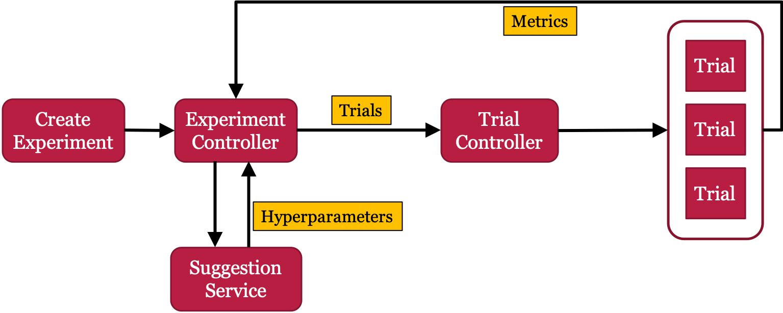
As shown in the schematic of Katib in Figure 10, an experiment is created and a handle to the experiment is sent to the Experiment Controller, which uses a Suggestion Service to get suggestions for hyperparameters. These hyperparameters along with the actual ML code form the trials, which are then run by a Trial Controller. The Trial Controller runs the trials on the underlying Kubernetes platform, collects the metrics of the run and feeds the metrics back to the Experiment Controller, which then continues the experiment with the next set of hyperparameter suggestions from the Suggestion Service. The Suggestion Service supports standard search methods and can also be fitted with custom search algorithms. Even though we use Katib in this paper, other hyperparameter optimization frameworks, such as Hyperopt [27], could be used as well.

-B Kubeflow: The Machine Learning toolkit for Kubernetes

Kubeflow [26] is an open-source project that makes the deployment of ML workflows on any Kubernetes installation simple, portable, and scalable. It supports running ML jobs written in frameworks such as TensorFlow [24] and PyTorch [25] and is extensible to any other framework. It is one of the most popular open-source project for managing ML workflows with contributors from a large number of companies. Even though Katib can be used independently we use Katib on top of Kubeflow since it eases the experimentation process.

References

- [1] H. Liu, H. Darabi, P. Banerjee, and J. Liu, “Survey of Wireless Indoor Positioning Techniques and Systems,” IEEE Transactions on Systems, Man, and Cybernetics, Part C (Applications and Reviews), vol. 37, no. 6, pp. 1067–1080, Nov 2007.
- [2] P. Bahl and V. N. Padmanabhan, “RADAR: An in-building RF-based user location and tracking system,” in Proceeding of IEEE INFOCOM, vol. 2, 02 2000, pp. 775 – 784.
- [3] A. Zhang, Y. Yuan, Q. Wu, S. Zhu, and J. Deng, “Wireless localization based on rssi fingerprint feature vector,” International Journal of Distributed Sensor Networks, vol. 11, no. 11, p. 528747, 2015. [Online]. Available: https://doi.org/10.1155/2015/528747
- [4] X. Zhao, Z. Xiao, A. Markham, N. Trigoni, and Y. Ren, “Does BTLE measure up against WiFi? A comparison of indoor location performance,” in European Wireless 2014; 20th European Wireless Conference, May 2014, pp. 1–6.
- [5] R. Faragher and R. Harle, “Location Fingerprinting With Bluetooth Low Energy Beacons,” IEEE Journal on Selected Areas in Communications, vol. 33, no. 11, pp. 2418–2428, Nov 2015.
- [6] P. Kriz, F. Maly, and K. Tomáš, “Improving indoor localization using bluetooth low energy beacons,” Mobile Information Systems, vol. 2016, pp. 1–11, 04 2016.
- [7] S. Bozkurt, G. Elibol, S. Gunal, and U. Yayan, “A comparative study on machine learning algorithms for indoor positioning,” in 2015 International Symposium on Innovations in Intelligent SysTems and Applications (INISTA), Sep. 2015, pp. 1–8.
- [8] A. H. Salamah, M. Tamazin, M. A. Sharkas, and M. Khedr, “An enhanced wifi indoor localization system based on machine learning,” in 2016 International Conference on Indoor Positioning and Indoor Navigation (IPIN), Oct 2016, pp. 1–8.
- [9] W. Zhang, K. Liu, W. Zhang, Y. Zhang, and J. Gu, “Deep neural networks for wireless localization in indoor and outdoor environments,” Neurocomput., vol. 194, no. C, pp. 279–287, Jun. 2016. [Online]. Available: https://doi.org/10.1016/j.neucom.2016.02.055
- [10] C. Shorten and T. M. Khoshgoftaar, “A survey on image data augmentation for deep learning,” Journal of Big Data, vol. 6, no. 1, p. 60, Jul 2019. [Online]. Available: https://doi.org/10.1186/s40537-019-0197-0
- [11] [Online]. Available: https://www.kaggle.com/
- [12] [Online]. Available: https://www.kaggle.com/ryches/better-indoor-localization-wip?scriptVersionId=10489664
- [13] I. Goodfellow, Y. Bengio, and A. Courville, Deep Learning. MIT Press, 2016, http://www.deeplearningbook.org.
- [14] J. Bergstra, D. Yamins, and D. D. Cox, “Making a science of model search: Hyperparameter optimization in hundreds of dimensions for vision architectures,” in Proceedings of the 30th International Conference on International Conference on Machine Learning - Volume 28, ser. ICML’13. JMLR.org, 2013, pp. I–115–I–123. [Online]. Available: http://dl.acm.org/citation.cfm?id=3042817.3042832
- [15] M. Mohammadi and A. Al-Fuqaha. (2018) BLE RSSI Dataset for Indoor localization and Navigation Data Set. Machine Learning Repository, University of California, Irvine. [Online]. Available: https://archive.ics.uci.edu/ml/datasets/BLE+RSSI+Dataset+for+Indoor+localization+and+Navigation#
- [16] M. Mohammadi, A. Al-Fuqaha, M. Guizani, and J. Oh, “Semisupervised Deep Reinforcement Learning in Support of IoT and Smart City Services,” IEEE Internet of Things Journal, vol. 5, no. 2, pp. 624–635, April 2018.
- [17] Kubernetes: Production-Grade Container Orchestration. [Online]. Available: https://kubernetes.io/
- [18] Keras: The Python Deep Learning library. [Online]. Available: https://keras.io/
- [19] Docker: Enterprise Container Platform. [Online]. Available: https://www.docker.com/
- [20] D. Kingma and J. Ba, “Adam: A method for stochastic optimization,” International Conference on Learning Representations, 12 2014.
- [21] [Online]. Available: https://en.wikipedia.org/wiki/Stochastic_gradient_descent
- [22] Katib in Kubeflow. [Online]. Available: https://github.com/kubeflow/katib
- [23] D. Golovin, B. Solnik, S. Moitra, G. Kochanski, J. Karro, and D. Sculley, “Google vizier: A service for black-box optimization,” in Proceedings of the 23rd ACM SIGKDD International Conference on Knowledge Discovery and Data Mining, ser. KDD ’17. New York, NY, USA: ACM, 2017, pp. 1487–1495. [Online]. Available: http://doi.acm.org/10.1145/3097983.3098043
- [24] TensorFlow: An open source machine learning framework for everyone. [Online]. Available: https://www.tensorflow.org/
- [25] PyTorch: A deep learning framework for fast, flexible experimentation. [Online]. Available: https://pytorch.org/
- [26] Kubeflow: The Machine Learning Toolkit for Kubernetes. [Online]. Available: https://github.com/kubeflow/kubeflow
- [27] Distributed Asynchronous Hyperparameter Optimization in Python. [Online]. Available: https://github.com/hyperopt/hyperopt