Calibrating Deep Neural Network Classifiers on Out-of-Distribution Datasets

Abstract

To increase the trustworthiness of deep neural network (DNN) classifiers, an accurate prediction confidence that represents the true likelihood of correctness is crucial. Towards this end, many post-hoc calibration methods have been proposed to leverage a lightweight model to map the target DNN’s output layer into a calibrated confidence. Nonetheless, on an out-of-distribution (OOD) dataset in practice, the target DNN can often mis-classify samples with a high confidence, creating significant challenges for the existing calibration methods to produce an accurate confidence. In this paper, we propose a new post-hoc confidence calibration method, called CCAC (Confidence Calibration with an Auxiliary Class), for DNN classifiers on OOD datasets. The key novelty of CCAC is an auxiliary class in the calibration model which separates mis-classified samples from correctly classified ones, thus effectively mitigating the target DNN’s being confidently wrong. We also propose a simplified version of CCAC to reduce free parameters and facilitate transfer to a new unseen dataset. Our experiments on different DNN models, datasets and applications show that CCAC can consistently outperform the prior post-hoc calibration methods.

1 Introduction

In recent years, classifiers based on deep neural networks (DNNs) have been increasingly applied to a wide variety of applications, including safety-critical applications [11, 19, 12] such as autonomous/assisted driving [3] and medical imaging [44, 5]. For trustworthiness, a quantitative confidence level should also be provided along with predicted labels of DNN classifiers, representing the actual likelihood of correctness of the corresponding classification result during inference [18, 26, 28, 46, 35]. Taking assisted driving as an example, a car may slow down and request human intervention in the event of a low-confidence prediction, ensuring a higher level of trustworthiness and safety.

Typically, for a DNN classifier with $K$ classes, the last layer contains $K$ neurons that correspond to a $K$-dimensional array of prediction probabilities (or a $K$-dimensional logit array, which can be converted into probabilities via softmax function), with the predicted class being the one that has the maximum prediction probability [16]. Straightforwardly, a prediction confidence can be directly obtained as the softmax probability for the predicted class [20]. Nonetheless, oftentimes, this naive un-calibrated confidence may not reveal the true prediction confidence, especially for modern complex DNN models. The mismatch between the softmax probability and the true prediction confidence can be attributed to over-fitting, batch normalization layers, among others [18].

Even worse, the actual target test dataset on which a DNN is applied in practice is often out-of-distribution (OOD) compared to the original dataset used to train the target DNN [46, 17, 20]. For example, in image classification, the actual images may be rotated and shifted, come from completely different domains with unseen labels, and/or even be modified by adversaries, which we broadly refer to as OOD samples in this paper. Importantly, recent studies have shown that the commonly-encountered OOD samples can cause a considerably large accuracy degradation and lead to over-confident predictions, thus presenting a significant challenge to the confidence of DNN prediction results and raising trust concerns [46]. While proactively detecting OOD samples to single them out may help prevent accuracy degradation [32, 35, 2, 6], not all OOD samples are mis-classified and hence a quantitative prediction confidence is still desired [46].

To obtain a prediction confidence that well represents the true likelihood of correctness, the target DNN model can be re-trained with a modified structure or training algorithm, such as Monte-Carlo dropout, SWAG, and deep ensembles [29, 13, 22], which are substitutes of otherwise computationally expensive Bayesian DNNs [24]. Nonetheless, re-trained DNNs may not guarantee an accurate prediction confidence on an actual test dataset with OOD samples, and it can be expensive or even impossible to re-train them each time the test data distribution changes. Alternatively, post-hoc confidence calibration [40, 18, 26] has been widely studied, which learns a lightweight model/network to map the target DNN’s output layer into a calibrated confidence score without re-training the DNN or modifying its architecture. Nonetheless, the calibrated confidence can be far off from the true likelihood of correct prediction for OOD samples in practical test datasets when the target DNN is often confidently wrong [46].

Our contribution. We study post-hoc confidence calibration for a DNN classifier when the actual test dataset can be possibly OOD (compared to the dataset used to train the target DNN). We propose a new post-hoc confidence calibration method, called CCAC (Confidence Calibration with an Auxiliary Class), which building on top of a lightweight (e.g., 2-layer) neural network, only needs the target DNN’s logit layer as input and maps it to a new calibrated softmax probability which can be used to indicate the prediction confidence. The key novelty of CCAC is the introduction of an auxiliary class which represents mis-classified samples and separates them from correctly classified ones in the actual test dataset, thus effectively mitigating the target DNN’s being confidently wrong (i.e., assigning a high confidence for mis-classified samples). To reduce the number of free parameters in CCAC, we propose a further simplified calibration model, called CCAC-S (CCAC-Simplified) as illustrated in Fig. 4(b), which uses a single temperature parameter to map the target DNN’s logit for correct classes in addition to leveraging a small neural network for the mis-classification class. More importantly, given a new unseen OOD test dataset in practice, we can transfer CCAC to the test dataset by using only a small number of newly labeled samples.

To evaluate the calibration performance, we conduct experiments for different DNNs on OOD datasets with both image and document classification applications (e.g., VGG16 on CIFAF-100 for image classification). The results show that our approach can consistently outperform recent post-hoc calibration methods in terms of the widely-used metrics of expected calibration error and Brier score, supporting the introduction of an auxiliary class to represent mis-classified samples to achieve a better confidence on OOD datasets.

2 Related Work

Confidence estimation. Most conventional DNN models do not provide accurate prediction uncertaintities/confidences [46]. While Bayesian DNN is an effective approach for uncertainty estimation, it requires significant modifications to the training procedure and suffers from a high computational cost for inference [24]. Consequently, novel DNN models and training algorithms, such as SWAG model [22], deep ensemble models [29] and Monte-Carlo dropout [13], have also been proposed to re-train DNNs as an approximate Bayesian approach. Nonetheless, these methods require a large training dataset and apply well each time the test data distribution changes. They are complementary to and can be applied in combination with post-hoc calibration methods (e.g., applying temperature scaling for each of the DNN models in an ensemble). Additionally, without model re-training, [45] proposes to re-sample weights in a DNN model as a Bayesian estimation, and [23] estimates prediction uncertainty using a trust score based on a ratio of the distance between a sample and its closest class to the distance between this sample and its predicted class. These methods also require the original training dataset and hence can only work well for in-distribution datasets.

Post-hoc confidence calibration. Without modifying an already-trained target DNN model, post-hoc confidence calibration can provide an accurate estimate of the prediction uncertainty by learning a mapping function from the model’s logit or probability output to a new probability that better represents the actual confidence. Typically, post-hoc calibration models, such as platter scaling [40], temperature scaling, vector scaling and matrix scaling [18], require a set of parameters that can be learnt via minimizing a certain loss function (e.g., negative log-likelihood or NLL) over a training/validation dataset. More recently, [26] proposes a sophisticated scaling method with Dirichlet functions and NLL loss for post-hoc calibration. Non-parametric calibration methods also exist, including binning methods [47] and isotonic regression method [48]. Moreover, some mixture methods are also proposed, including Bayesian binning [37] and scaling binning [28]. However, the existing post-hoc calibration methods are mainly developed for in-distribution datasets and, as empirically shown in a recent study [46], cannot calibrate the prediction confidence well for OOD datasets. Our proposed calibration method falls into post-hoc calibration but can provide a good calibration performance on an actual test dataset that typically includes OOD samples.

OOD/adversarial/misclassification detection. A simple baseline method using softmax probability (plus some hidden layers as an extension) for misclassification/OOD detection is considered in [20]. Following up, [32] detects OOD samples using temperature scaling and input perturbations, [30] studies OOD detection by learning a generative model based on hidden layers of a white-box DNN, [2] extracts features from inner layers for OOD detection in white-box DNNs, [6] trains a deep verifier (generative neural network) based on raw input data for OOD and misclassification detection, [35] proposes a prior network to better separate OOD/adversarial samples from in-distribution/benign samples, and [36] uses self-supervised learning to jointly detect OOD and train the target DNN model. Another related line of research is learning with rejection [9, 10, 14], where the classifier is trained along with a rejection score function such that the classifier can selectively provide predictions based on the corresponding rejection score. While these methods can single out OOD/adversarial samples (and sometimes mis-classified samples), they cannot provide a quantitative prediction confidence on OOD/adversarial samples, which may still be correctly classified by the target DNN.

3 Confidence Calibration With an Auxiliary Class

3.1 Problem Formulation

We consider a DNN classifier $\mathcal{F}_{\Theta}(\mathbf{x})$ with $K$ classes, where $\mathbf{x}$ is the input data with a true label $y$ and $\Theta$ represents the model parameters learned from labeled training samples in dataset $\mathcal{D}^{T}$. The model parameters $\Theta$ are not required nor modified by post-hoc confidence calibration methods [18].

The actual test data $(\mathbf{x},y)$ is drawn from a dataset $\mathcal{D}$, whose data distribution may differ from that of the dataset $\mathcal{D}^{T}$ used for training the target DNN. Given an input $\mathbf{x}$, the target DNN’s logit output is denoted by $\mathbf{z}\in\mathbb{R}^{K}$, where we suppress the dependence of $\mathbf{z}(\mathbf{x})$ on $\mathbf{x}$ for notational convenience. The corresponding output probability is $\mathbf{p}(\mathbf{z})=\sigma_{SM}(\mathbf{z})\in\mathbb{R}^{K}$, where $\sigma_{SM}$ is the softmax function. The predicted label $\hat{y}$ is decided as $\hat{y}=\arg\max_{k\in\{1,2...K\}}\{{p}_{k}(\mathbf{z})\}$. The classification is correct when $\hat{y}=y$ and wrong otherwise, with $\mathrm{Pr}(\hat{y}=y)=\max_{k\in\{1,2...K\}}\{{p}_{k}(\mathbf{z})\}$ being the (un-calibrated) classification confidence. Ideally, the confidence $\mathrm{Pr}(\hat{y}=y)$ should reflect the true probability of correct classification [18]. For example, given $R$ samples samples each with a prediction confidence of $q$, the correctly predicated samples should be $R\cdot q$. Nonetheless, the un-calibrated prediction confidence of a DNN classifier can differ significantly from the true confidence, especially on OOD datasets [46].

The goal of post-hoc confidence calibration is to map the logit $\mathbf{z}$ (or the softmax probability $\mathbf{p}(\mathbf{z})=\sigma_{SM}(\mathbf{z})$) of the target DNN into a calibrated confidence that better represents the true confidence.

3.2 Confidence Calibration

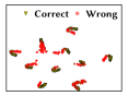
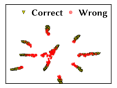
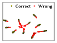
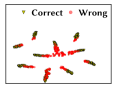
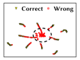
Figure 1: t-SNE of calibrated confidence for VGG16 on CIFAR-10 OOD dataset. (a) Un-calibrated. (b) Temperature scaling. (c) Scaling-binning. (d) Dirichlet calibration. (e) CCAC.

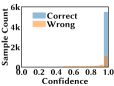
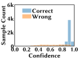
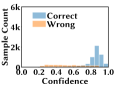
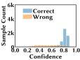
Figure 2: Histograms of prediction confidences for VGG16 on CIFAR-10 OOD dataset. (a) Un-calibrated. (b) Temperature scaling. (c) Scaling-binning. (d) Dirichlet calibration. (e) CCAC.

Before describing CCAC, we first review the confidences calibrated by some recent methods — temperature scaling [18], scaling-binning [28], and Dirichlet calibration [26] — whose details are further described in Section 4.1.1. Concretely, for presentation clarity, we randomly select 50 samples from each class and show in Fig. 1 the t-SNE visualization [34] of both un-calibrated and calibrated softmax probabilities on CIFAR-10 OOD dataset (whose details are available in our experiment results). We notice from Figs. 1–1 that while the softmax probabilities of different classes are well separated, wrong samples are still largely mixed together with correct samples for each class. This is not surprising, since mis-classified samples may not be corrected by confidence calibration alone (e.g., calibration using temperature scaling still preserves the original predicted label [18]). By contrast, due to the introduction of an auxiliary class in CCAC, we see from Fig. 1 that mis-classified samples tend to be more separated from correctly classified ones as a single cluster. This point is also reaffirmed in Fig. 2, where we show the histogram of calibrated confidences. It can be seen that many mis-classfied samples still have a high calibrated confidence by using the existing calibration methods, whereas they tend to have a much lower calibrated confidence by using CCAC.

Overview of CCAC. From the above analysis, we see that assigning a high confidence to mis-classified samples is a major cause for poor calibration on OOD datasets [46]. To avoid being confidently wrong, we cannot identify true labels for those mis-classified samples by only using calibration, since post-hoc calibration is not designed for this purpose. Instead, we propose CCAC (Confidence Calibration with an Auxiliary Class), which separates mis-classified samples from correctly classified ones, such that mis-classified samples can be assigned with a low confidence. To accomplish this, we add an auxiliary class to represent samples that are mis-classified by the target DNN, and train a model to map the logit $\mathbf{z}\in\mathbb{R}^{K}$ (produced by the target DNN) to a calibrated probability $\mu(\mathbf{z})\in\mathbb{R}^{K+1}$. Specifically, in CCAC, $\mu_{k}(\mathbf{z})$ and $\mu_{K+1}(\mathbf{z})$ represent the likelihoods of class $k$ (for $k=1,\cdots,K$) and mis-classification, respectively, with $\sum_{k=1}^{K+1}\mu_{k}(\mathbf{z})=1$. Then, by combining the calibrated probabilities for both the predicted label and mis-classification, we obtain the calibrated confidence. Our design of CCAC is also illustrated in Fig. 4.

Loss function for CCAC. Given the target DNN’s $K$-dimensional logit $\mathbf{z}$, our calibration model maps $\mathbf{z}$ to a $(K+1)$-dimensional calibrated softmax probability $\mu(\mathbf{z})$. In CCAC, we extend the original $K$-class label $y$ to a $(K+1)$-class label $w$, which includes the same set of $K$ original classes and an additional auxiliary class $K+1$ that represents samples mis-classified by the target DNN. Specifically, if a sample $(\mathbf{x},y)$ belonging to class $k$ is correctly classified by the target DNN, its label $w$ in CCAC is still class $k$ (i.e., $w=y$); otherwise, its label $w$ becomes “class $(K+1)$” (i.e., class of mis-classified samples). We use one-hot encoding $\mathbf{w}=[w_{1},\cdots,w_{K+1}]$ to represent the label in CCAC, i.e., $w_{k}=1$ if the sample belongs to class $k$ and $w_{k}=0$ otherwise, for $k=1,\cdots,K+1$. We consider the following cross-entropy loss:

$$\mathcal{L}=-\sum_{k=1}^{K+1}w_{k}\log\left({\mu}_{k}\right),$$ (1)

where $\mu_{k}$ is the calibrated softmax probability $\mu(\mathbf{z})$ for a sample belonging to class $k$ in CCAC.

In Eqn. (1), some correctly classified samples can also have a large probability $\mu_{K+1}$ of being considered as mis-classified. To prevent correctly classified samples from having a large $\mu_{K+1}$, we can modify the loss by adding a regularization term $-(1-w_{K+1})\log(1-{\mu}_{K+1})$ into the loss function. For a correctly classified sample, we have $w_{k}=1$ for its true class and meanwhile $w_{K+1}=0$. Thus, the added regularization $-(1-w_{K+1})\log(1-{\mu}_{K+1})$ is only effective for correctly classified samples and aims at pushing them away from class $K+1$ (i.e., reducing $\mu_{K+1}$). Additionally, we can add another weight for the auxiliary class $K+1$. Thus, we consider a modified loss function as follows:

$$\mathcal{L}=-\sum_{k=1}^{K}w_{k}\log\left({\mu}_{k}\right)-\lambda_{1}(1-w_{K+1})\log(1-{\mu}_{K+1})-\lambda_{2}w_{K+1}\log\left({\mu}_{K+1}\right),$$ (2)

where $\lambda_{1}\geq 0$ and $\lambda_{2}\geq 0$ are tunable hyperparameters.

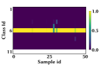
(a) Un-calibrated

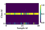
(b) Calibrated by CCAC

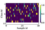
(c) Un-calibrated

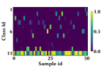
(d) Calibrated by CCAC

Figure 3: Softmax probabilities for VGG16 on CIFAR-10 OOD dataset. (a)(b) Results for 50 correctly classified samples in class 6. (c)(d) Results for 50 mis-classified samples.

Next, we highlight the importance of our introduced auxiliary class by showing in Fig. 3 the uncalibrated/calibrated probabilities for 50 correctly classified samples (belonging to one class) and 50 mis-classified samples. We see that after calibration by CCAC, the correctly classified samples can largely keep their high probabilities for the true class. On the other hand, CCAC can significantly reduce the probabilities of false classes for mis-classified samples, pushing mis-classified samples to have a high $\mu_{K+1}$ and effectively mitigating “confidently wrong”.

Calibrated confidence. If all samples mis-classified by the target DNN are perfectly identified and assigned with $\mu_{K+1}=1$, then we could directly use $\mu_{k}$ as the calibrated confidence. But, this is not practically possible. Here, without modifying the original prediction label, we propose to combine $\mu_{K+1}$ together with the calibrated softmax probability $\mu_{\hat{y}}$ for the label $\hat{y}\in\{1,\cdots,K\}$ predicted by the target DNN. Specifically, we consider two different types of geometric means for the calibrated confidence:

$$confidence=1-\sqrt{(1-\mu_{\hat{y}})\mu_{K+1}}\text{\;\;\;\; and \;\;\;\;}confidence=\sqrt{\mu_{\hat{y}}(1-\mu_{K+1})}.$$ (3)

The interpretation for $confidence=1-\sqrt{(1-\mu_{\hat{y}})\mu_{K+1}}$ is as follows: given a sample classified by the target DNN as class $\hat{y}$, $1-\mu_{\hat{y}}$ and $\mu_{K+1}$ can both represent the probability of mis-classification, $\sqrt{(1-\mu_{\hat{y}})\mu_{K+1}}$ is the geometric mean, and hence $1-\sqrt{(1-\mu_{\hat{y}})\mu_{K+1}}$ can be used as a calibrated confidence. The interpretation for $confidence=\sqrt{\mu_{\hat{y}}(1-\mu_{K+1})}$ is also similar.

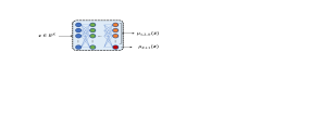
(a) CCAC

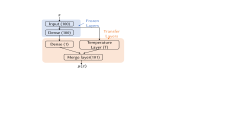
(b) CCAC-S

Figure 4: Overview of our confidence calibration models.

Training of CCAC. As shown in Fig. 4(a), we can use a neural network for minimizing the loss. Specifically, with labeled samples from the actual test dataset to which the target DNN is applied, we adopt standard training algorithms to construct the neural network. Suppose that CCAC uses $L$ fully connected layers each with $K$ nodes. Then, given $K$ put nodes and $K+1$ output nodes, CCAC needs to learn $\sim O(LK^{2})$ weight parameters. Additionally, we also use a small validation dataset for tuning hyperparameters and deciding which of two calibrated confidences in Eqn. (3) to use.

Simplified CCAC and transfer. When applying the target DNN to a new test dataset, labeling samples to learn $\sim O(LK^{2})$ weight parameters in CCAC may be too expensive. Thus, to reduce the number of labeled samples needed, we propose a simplified calibration model, called CCAC-S (CCAC-Simplified), which is illustrated in Fig. 4(b). Specifically, the logit input $\mathbf{z}$ is scaled using a temperature parameter $T$ for the first $K$ classes in CCAC-S, and the logit for the $(K+1)$-th class is obtained using a neural network. Then, the $K+1$ logits are merged together, based on which the calibrated softmax probability $\mu$ is derived. Note that for training both CCAC and CCAC-S, we assign “class $(K+1)$” to samples mis-classified by the target DNN, while keeping the labels of those correct samples unchanged.

Another advantage of CCAC-S is its easy transferability. Specifically, we can first train CCAC-S on a given labeled dataset. Then, when applying the target DNN to a new unseen dataset, we freeze all the parameters in CCAC-S, except for the temperature parameter $T$ (for the first $K$ classes) and the last fully connected layer in the neural network (for the $(K+1)$-th class). Suppose that the penultimate layer in the neural network has $K$ nodes. We only need to learn a total of $K+2$ weight parameters (temperature plus $K+1$ parameters for the last layer), which requires significantly fewer samples than learning weights for CCAC and CCAC-S from scratch. Thus, for a new unseen dataset, we only need to label a small set of samples from the target test dataset.

4 Experiments

We conduct experiments for different DNNs on various datasets with both image and document classification applications. The results show that our approach can consistently outperform recent post-hoc calibration methods in terms of the calibration performance.

4.1 Methodologies

We train both CCAC and CCAC-S in Tensorflow [1] with Keras layers [8]. All experiments are executed within Jupiter Notebook under the Anaconda environment.

4.1.1 Baseline Approaches

Our proposed method belongs to post-hoc confidence calibration. Thus, for fair comparison, we consider the following state-of-the-art post-hoc calibration approaches as baselines.

Max probability (MP): The prediction confidence by MP is not calibrated and directly calculated as $MP=\max_{k\in\{1,2...K\}}\{{p}_{k}\}$, where $p_{k}$ is the target DNN’s softmax probability for class $k$ [20].

Temperature scaling (TS): TS provides calibrates confidence by learning a single multiplicative factor $T$ (a.k.a. scaling temperature) on the target DNN’s logit output z [18]. The calibrated confidence ${p}_{T}$ can be presented as ${p}_{T}=\max\sigma_{SM}(\textbf{z}/T)$. We learn the temperature $T$ in TS by minimizing a negative log-likelihood (NLL) loss [18].

Scaling-binning (SB): The SB calibrator combines two popular post-hoc calibration methods: platter scaling and histogram binning [28]. Like in TS, we also use the same dataset utilized for training CCAC to train the calibration function for each bin in SB. Dirichlet calibration: The recently proposed Dirichlet calibration [26] extends Beta calibration [27] to $K$-class classifiers. Specifically, a calibration model is learned to map $K$-dimensional the un-calibrated softmax probability p into a well-calibrated confidence/probability ${\mu}(\textbf{p})$. The mapping function includes $K$ Dirichlet functions with $O(K^{2})$ parameters learnt by minimizing the NLL loss.

4.1.2 Evaluation Metrics

Confidence calibration metrics: We consider the commonly-used calibration metrics — expected calibration error (ECE) and Brier Score (BS) [26, 18]. Specifically, the test samples are firstly grouped into $M$ equal-width bins according to their (calibrated) confidence scores. Within the bin $B_{m},m\in\{1,2...M\}$, the average prediction accuracy $Acc(B_{m})$ and the average confidence $Conf(B_{m})$ can be empirically calculated as $Acc(B_{m})=\frac{1}{|B_{m}|}\sum_{i\in B_{m}}{\textbf{1}(\hat{y_{i}}=y_{i})}$ and $Conf(B_{m})=\frac{1}{|B_{m}|}\sum_{i\in B_{m}}{\hat{c_{i}}}$, respectively. Then, the ECE value can be calculated as the weighted-average of the absolute difference between $Acc(B_{m})$ and $Conf(B_{m})$, i.e., $ECE=\sum_{m1}^{M}\frac{|B_{m}|}{N}|Acc(B_{m})-Conf(B_{m})|$, where $N$ is the total number of test samples and $|B_{m}|$ represents the sample counts in bin $B_{m}$ [18]. In our experiments, we use $M=20$ bins for reliability diagrams and ECE calculation. The BS estimates the mean squared error between correctness of prediction and confidence score [4], and can be calculated as $BS(\mathcal{D})=\frac{1}{|\mathcal{D}|}\sum_{i\in\mathcal{D}}(\textbf{1}(\hat{y_{i}}=y_{i})-\hat{c_{i}})^{2}$, where $\hat{c_{i}}$ is the confidence for an input $\textbf{x}_{i}$, $\mathcal{D}$ represents the entire test dataset and $\textbf{1}(\hat{y_{i}}=y_{i})$ indicates if the classification for input $\textbf{x}_{i}$ is correct or not. For both ECE and BS metrics, the lower value, the better.

Misclassification detection metrics: While our main purpose is confidence calibration, a byproduct of our method is the better detection of mis-classified samples based on a threshold of the calibrated confidence. We consider AUROC (Area Under the Receiver Operating Characteristic) and AUPR (Area Under the Precision-Recall Curve) as metrics for mis-classification detection, since they are independent of the thresholds. A higher AUROC/AUPR implies a better distinguishability between correctly classified and mis-classified samples. In addition, we also use the precision at 90% recall (denoted as $\mathbf{p{.9}}$) as an evaluation metric, which represents the precision when we aim at detecting 90% of the mis-classified samples. Note that a mis-classified sample is treated as “positive” in mis-classification detection when calculating AUROC, AUPR and $\mathbf{p{.9}}$.

4.2 Results for Image Classification

We consider 10-class, 100-class and 1000-class image classifications.

4.2.1 10-class Image Classification with VGG16 DNN

Target DNN model. The target DNN model is a modified VGG16 for tiny images (CIFAR). The target model includes batch normalization layers and dropout layers to improve classification performance. It is trained in TensorFlow on CIFAR-10 training dataset (50k images). The pre-trained weights of target DNN model are downloaded from [15].

Datasets. We evaluate the calibration performance on four datasets generated from CIFAR-10 and CIFAR-100 [25], including two augmented datasets (D1 and D2), one out-of-distribution dataset (OOD) and one adversarial dataset (AD). We first randomly select 30k samples from CIFAR-10 training dataset and 10k samples from CIFAR-10 testing dataset, and then perform augmentation operations on the selected samples. For D1, the augment operations and parameters include rotation within $[-20,20]$ degrees, vertical/horizontal shift within $[-0.25,0.25]$, zoom with $0.4$, and horizontal flip. For D2, the augmentation parameters are: rotation within $[-40,40]$ degrees, vertical/horizontal shift within $[-0.4,0.4]$, zoom with $0.5$, and horizontal flip. The OOD dataset also includes 40k samples, with 12k OOD samples randomly selected from CIFAR-100 training dataset and 28k samples from CIFAR-10 training dataset. As for 12k OOD samples from CIFAR-100, the true labels are mapped to CIFAR-10’s class labels. Specifically, we consider OOD samples with label “pick-up truck” as “truck” in CIFAR-10 and OOD samples with label “automobile” as “bus” in CIFAF-10. The other OOD samples are treated with “NULL” label, indicating not belonging to any of the 10 classes in CIFAR-10. For the AD dataset, the 40k samples include 20k normal samples and 20k adversarial samples. The 20k normal samples contain 10k images from the CIFAR-10 training dataset and 10k images from the CIFAR-10 testing dataset, while the 20k adversarial samples are generated based on 20k randomly selected samples from the CIFAR-10 training dataset with DeepFool-Attack using foolbox package [41]. The inference accuracies on the four test datasets are 80% (D1), 62% (D2), 71% (OOD), and 47% (AD). Additionally, the 40k samples (in D1, D2, OOD or AD) are randomly split into a 30k dataset for training, a 2k validation dataset for hyperparameter tuning, and a 8k testing dataset for performance evaluation.

Baselines. For each dataset, the baselines of TS, SB, and Dirichlet calibration are trained on the respective 30k training dataset. For Dirichlet calibration, the regularization hyperparameters are tuned with a minimal ECE on the 2k validation dataset. The 30k training and 2k validation datasets are the same as those used for training CCAC and CCAC-S.

Our method. The neural network of CCAC is implemented with 2 hidden layers, including 50 hidden neurons in first hidden layer and 20 hidden nodes in the second layer. The input layer contains 10 nodes and the output layer contains 11 nodes (including 10 classes and one “mis-classification” class). CCAC is trained over 1000 epochs using the Adam optimizer (learning rate $10^{-3}$). The loss function hyperparameters ($\lambda_{1}$ and $\lambda_{2}$) and the confidence calculation method are selected with a minimal ECE on the validation dataset. For CCAC-S, the neural network is implemented with the same structure as CCAC, but the output layer contains only 1 node, representing the “mis-classification” class. The temperature scaling layer is implemented with a self-defined customer Keras layer with one learnable weight $T$. The training settings of CCAC-S are the same as those of CCAC. For the transferred model CCAC-T, we first pre-train CCAC-S on dataset D1. Then, when applied to another target dataset, a set of 320 samples are randomly selected from the respective 30k training dataset for model transfer. In addition, we select another 200 samples from the 2k validation dataset to tune corresponding hyperparameters and confidence calculation method in CCAC-T.

Table 1: VGG16 on CIFAR-10 D1

Method	AUROC	AUPR	p.9	ECE	BS
MP	0.865	0.566	0.419	13.9%	0.151
TS	0.870	0.586	0.421	4.6%	0.116
SB	0.872	0.589	0.429	2.9%	0.113
Dirichlet	0.870	0.586	0.422	4.5%	0.116
CCAC	0.907	0.715	0.489	1.4%	0.095
CCAC-S	0.906	0.696	0.493	1.9%	0.097
CCAC-T	-	-	-	-	-

Table 2: VGG16 on CIFAR-10 D2

Method	AUROC	AUPR	p.9	ECE	BS
MP	0.814	0.664	0.560	28.2%	0.280
TS	0.823	0.677	0.573	9.2%	0.174
SB	0.839	0.688	0.606	3.6%	0.158
Dirichlet	0.823	0.677	0.574	8.7%	0.173
CCAC	0.879	0.773	0.649	2.3%	0.137
CCAC-S	0.878	0.764	0.652	3.0%	0.138
CCAC-T	0.876	0.775	0.642	3.8%	0.140

Table 3: VGG16 on CIFAR-10 OOD

Method	AUROC	AUPR	p.9	ECE	BS
MP	0.923	0.816	0.640	24.3%	0.225
TS	0.927	0.833	0.650	14.4%	0.140
SB	0.921	0.834	0.604	11.8%	0.119
Dirichlet	0.923	0.816	0.640	15.9%	0.126
CCAC	0.940	0.870	0.674	2.0%	0.087
CCAC-S	0.934	0.861	0.645	2.0%	0.091
CCAC-T	0.894	0.802	0.512	3.1%	0.108

Table 4: VGG16 on CIFAR-10 AD

Method	AUROC	AUPR	p.9	ECE	BS
MP	0.923	0.889	0.839	48.9%	0.461
TS	0.913	0.885	0.825	34.1%	0.230
SB	0.890	0.876	0.770	20.5%	0.197
Dirichlet	0.685	0.657	0.625	8.8%	0.220
CCAC	0.935	0.926	0.856	3.5%	0.097
CCAC-S	0.934	0.925	0.860	3.3%	0.098
CCAC-T	0.872	0.864	0.749	3.8%	0.143

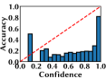
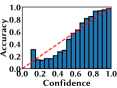
Figure 5: Reliability diagrams of prediction confidences for VGG16 on CIFAR-10 OOD dataset. (a) Un-calibrated. (b) Temperature scaling. (c) Scaling-binning. (d) Dirichlet calibration. (e) CCAC.

Results. The calibration results are presented in Table 2, 2, 4 , 4 for D1, D2, OOD and AD datasets, respectively. We highlight the best performance among all the calibration methods with bold font, including the highest AUROC/AUPR/p.9 for mis-classification detection and the lowest ECE/BS for confidence calibration. The results show that the proposed methods (CCAC, CCAC-S) outperform the baselines in terms of both mis-classification detection and confidence calibration, with more significant improvement on OOD and AD datasets. In addition, even though CCAC-T model is transferred to D2/OOD/AD datasets with fewer training samples than the baselines, it still offers a better calibration performance in terms of ECE and BS.

We further show the histograms of confidences for correct and wrong predictions in Fig. 2 on the OOD dataset. The corresponding reliability diagrams also are shown in Fig. 5 on the OOD dataset with different calibration methods. Without calibration, most confidences are high ($\sim 1.0$) for correct and wrong predictions, resulting in confidently wrong predictions and over-confident reliability diagrams. While reducing the confidence for mis-classified samples, the baseline calibration methods also tend to decrease the confidences of correct predictions. The reliability diagrams shows over-confidence for low confidences, and slight under-confidence for high confidences. Nevertheless, CCAC can provide better calibration performance by separating mis-classified samples from correctly sampled ones.

Table 5: ResNet-50 on CIFAR-10 D1

Method	AUROC	AUPR	p.9	ECE	BS
MP	0.834	0.576	0.430	16.8%	0.182
TS	0.833	0.575	0.427	4.4%	0.139
SB	0.843	0.585	0.438	4.7%	0.137
Dirichlet	0.833	0.575	0.427	4.3%	0.139
CCAC	0.853	0.605	0.457	2.3%	0.132
CCAC-S	0.853	0.604	0.458	1.4%	0.130
CCAC-T	-	-	-	-	-

Table 6: ResNet-50 on CIFAR-10 D2

Method	AUROC	AUPR	p.9	ECE	BS
MP	0.785	0.665	0.551	29.1%	0.292
TS	0.784	0.668	0.546	3.8%	0.186
SB	0.792	0.668	0.560	3.9%	0.183
Dirichlet	0.784	0.668	0.546	3.8%	0.186
CCAC	0.811	0.692	0.590	3.4%	0.037
CCAC-S	0.813	0.692	0.589	2.2%	0.172
CCAC-T	0.809	0.690	0.593	3.2%	0.174

Table 7: ResNet-50 on CIFAR-10 OOD

Method	AUROC	AUPR	p.9	ECE	BS
MP	0.883	0.761	0.548	25.0%	0.233
TS	0.879	0.752	0.535	9.0%	0.138
SB	0.886	0.779	0.545	7.4%	0.127
Dirichlet	0.875	0.746	0.529	7.6%	0.131
CCAC	0.913	0.832	0.615	1.8%	0.104
CCAC-S	0.890	0.785	0.552	1.6%	0.118
CCAC-T	0.874	0.761	0.520	1.9%	0.126

Table 8: ResNet-50 on CIFAR-10 AD

Method	AUROC	AUPR	p.9	ECE	BS
MP	0.730	0.604	0.421	27.8%	0.283
TS	0.724	0.603	0.412	6.4%	0.201
SB	0.752	0.616	0.452	4.9%	0.193
Dirichlet	0.724	0.603	0.412	6.5%	0.202
CCAC	0.780	0.654	0.481	2.5%	0.181
CCAC-S	0.783	0.663	0.479	2.0%	0.179
CCAC-T	0.732	0.581	0.433	4.5%	0.199

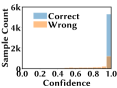
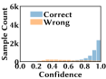
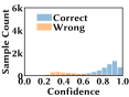
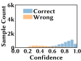
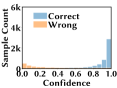
Figure 6: Histograms of prediction confidences for ResNet-50 on CIFAR-10 OOD dataset. (a) Un-calibrated. (b) Temperature scaling. (c) Scaling-binning. (d) Dirichlet calibration. (e) CCAC.

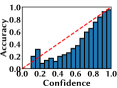
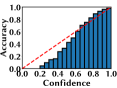
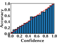
Figure 7: Reliability diagrams of prediction confidences for ResNet-50 on CIFAR-10 OOD dataset. (a) Un-calibrated. (b) Temperature scaling. (c) Scaling-binning. (d) Dirichlet calibration. (e) CCAC.

4.2.2 10-class Image Classification with ResNet-50 DNN

Target DNN model. The target DNN model is a modified ResNet-50 for tiny images (CIFAR). The target model includes batch normalization layers and dropout layers to improve classification performance. It is trained in PyTorch on CIFAR-10 training dataset (50k images). The pre-trained weights of target DNN model are downloaded from [7].

All the other settings, such as the datasets and architecture of the neural network in CCAC/CCAC-S, are the same as those for the 10-class VGG16 DNN described in Section 4.2.1. The inference accuracies on the four test datasets are 75% (D1), 59% (D2), 70% (OOD), and 63% (AD).

Results. The calibration results are presented in Table 6, 6, 8, 8 for D1, D2, OOD and AD datasets, respectively.

The results show that the proposed methods (CCAC, CCAC-S) outperform the baselines in terms of both mis-classification detection and confidence calibration, with significant improvement on OOD and AD datasets. We further show the histograms of confidences for correct and wrong predictions in Fig. 6 on the OOD dataset. The corresponding reliability diagrams also are shown in Fig. 7 on the OOD dataset with different calibration methods.

4.2.3 100-class Image Classification with VGG16 DNN

Target DNN model. The target DNN model is a modified VGG16 for tiny images (CIFAR). The target model includes batch normalization layers and dropout layers to improve classification performance. It is trained in Tensorflow on CIFAR-100 training dataset (50k images). The pre-trained weights of target DNN model is downloaded from [15].

Datasets. We evaluate the calibration performance on four datasets generated from CIFAR-100 and CIFAR-10 [25], including two augmented datasets (D1 and D2), one out-of-distribution dataset (OOD) and one adversarial dataset (AD). We first randomly select 30k samples from CIFAR-100 training dataset and 10k samples from CIFAR-100 testing dataset, and then perform augmentation operations on the selected samples. For D1, the augment operations and parameters include rotation within $[-20,20]$ degrees, vertical/horizontal shift within $[-0.25,0.25]$, zoom with $0.4$, and horizontal flip. For D2, the augmentation parameters are: rotation within $[-40,40]$ degrees, vertical/horizontal shift within $[-0.4,0.4]$, zoom with $0.5$, and horizontal flip. All augmentations are performed via ImageDataGenerator function in Tensorflow. The OOD dataset also includes 40k samples, with 12k OOD samples randomly selected from CIFAR-10 training dataset and 28k samples from CIFAR-100 training dataset. As for 12k OOD samples from CIFAF-10, the true labels are mapped to CIFAR-100’s class labels. Specifically, we consider OOD samples with label “truck” as “pick-up truck” in CIFAR-100, and OOD samples with label “bus” as “automobile” in CIFAR-100. The other OOD samples are considered with “NULL” labels, indicating not belonging to any of the 100 classes in CIFAR-100. For the AD dataset, the 40k samples include 20k normal samples and 20k adversarial samples. The 20k normal samples contain 10k images from the CIFAR-100 training dataset and 10k images from the CIFAR-100 testing dataset, while the 20k adversarial samples are generated based on 20k randomly selected samples from the CIFAR-100 training dataset with DeepFool-Attack using foolbox package [41]. The inference accuracies on the four test datasets are 65% (D1), 47% (D2), 77% (OOD), and 54% (AD). The 40k samples (in D1, D2, OOD or AD) are randomly split into a 30k dataset for training, a 2k validation dataset for hyperparameter tuning, and a 8k testing dataset for performance evaluation.

Baselines. For each dataset, the baselines of TS, SB, and Dirichlet calibration are trained on the respective 30k training dataset. For Dirichlet calibration, the regularization hyperparameters are tuned with a minimal ECE on the 2k validation dataset. The 30k training and 2k validation dataset are the same as those used for training CCAC and CCAC-S.

Our method. The neural network of CCAC is implemented with one hidden layers with 100 hidden nodes. The input layer contains 100 nodes and the output layer contains 101 nodes (including 100 classes and one “mis-classification” class). CCAC is trained over 1000 epochs using the Adam optimizer (learning rate $10^{-3}$). The loss function hyperparameters ($\lambda_{1}$ and $\lambda_{2}$) and the confidence calculation method are selected with a minimal ECE on the validation dataset. For CCAC, the neural network is implemented with the same structure as CCAC, but the output layer contains only 1 node, representing the “mis-classification” class. The temperature scaling layer is implemented with a self-defined customer Keras layer with one learnable weight $T$. The training settings of CCAC-S are the same as those of CCAC. For the transferred model CCAC-T, we first pre-train CCAC-S on dataset D1. Then, when applied to another target dataset, a set of 320 samples are randomly selected from the 30k training dataset for 30k training dataset . In addition, we select another 200 samples from the 2k validation dataset to tune corresponding hyperparameters and confidence calculation method in CCAC-T.

Results. The calibration results are presented in Table 10, 10, 12 , 12 for D1, D2, OOD and AD datasets, respectively. The results show that the proposed method (CCAC) outperforms the baselines in terms of mis-classification detection. For confidence calibration, the proposed methods provide the best calibrated confidence (lowest ECE) on D2, OOD and AD, with significant improvement on OOD and AD datasets. For D1, our proposed method achieves a well-calibrated confidence comparable to the best calibration. In addition, even though CCAC-T model is transferred to D2/OOD/AD datasets with fewer training samples than the baselines, it still offers a better calibration performance in terms of ECE. We further show the histograms of confidences for correct and wrong predictions in Fig. 8 on OOD dataset. The corresponding reliability diagrams also are shown in Fig. 9 on OOD dataset with different calibration methods.

Table 9: VGG16 on CIFAR-100 D1

Method	AUROC	AUPR	p.9	ECE	BS
MP	0.841	0.708	0.538	19.6%	0.206
TS	0.846	0.720	0.550	2.3%	0.151
SB	0.878	0.777	0.592	2.0%	0.135
Dirichlet	0.861	0.737	0.574	3.5%	0.144
CCAC	0.880	0.787	0.596	2.4%	0.134
CCAC-S	0.862	0.756	0.566	2.1%	0.136
CCAC-T	-	-	-	-	-

Table 10: VGG16 on CIFAR-100 D2

Method	AUROC	AUPR	p.9	ECE	BS
MP	0.800	0.790	0.683	31.8%	0.300
TS	0.813	0.805	0.690	2.5%	0.174
SB	0.852	0.848	0.734	2.7%	0.155
Dirichlet	0.840	0.829	0.724	4.4%	0.163
CCAC	0.865	0.867	0.741	1.6%	0.148
CCAC-S	0.851	0.851	0.726	1.7%	0.155
CCAC-T	0.846	0.841	0.725	2.4%	0.158

Table 11: VGG16 on CIFAR-100 OOD

Method	AUROC	AUPR	p.9	ECE	BS
MP	0.890	0.690	0.477	16.5%	0.161
TS	0.890	0.701	0.463	8.9%	0.122
SB	0.877	0.617	0.522	8.2%	0.128
Dirichlet	0.784	0.507	0.327	3.2%	0.145
CCAC	0.936	0.812	0.611	3.1%	0.087
CCAC-S	0.921	0.769	0.555	2.7%	0.094
CCAC-T	0.919	0.748	0.551	2.6%	0.095

Table 12: VGG16 on CIFAR-100 AD

Method	AUROC	AUPR	p.9	ECE	BS
MP	0.916	0.858	0.788	37.2%	0.333
TS	0.914	0.859	0.789	15.5%	0.146
SB	0.916	0.883	0.769	16.1%	0.158
Dirichlet	0.894	0.849	0.739	13.4%	0.153
CCAC	0.933	0.892	0.833	4.9%	0.100
CCAC-S	0.924	0.872	0.815	4.3%	0.106
CCAC-T	0.858	0.803	0.673	3.9%	0.153

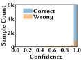
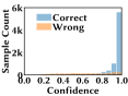
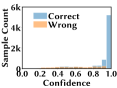
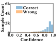
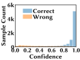
Figure 8: Histograms of prediction confidences for VGG16 on CIFAR-100 OOD dataset. (a) Un-calibrated. (b) Temperature scaling. (c) Scaling-binning. (d) Dirichlet calibration. (e) CCAC.

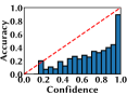
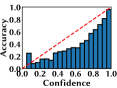
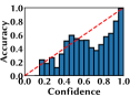
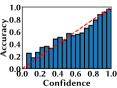
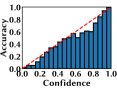
Figure 9: Reliability diagrams of prediction confidences for VGG16 on CIFAR-100 OOD dataset. (a) Un-calibrated. (b) Temperature scaling. (c) Scaling-binning. (d) Dirichlet calibration. (e) CCAC.

4.2.4 100-class Image Classification with ResNet-50 DNN

Target DNN model. The target DNN model is a modified ResNet-50 for tiny images (CIFAR). The target model includes batch normalization layers and dropout layers to improve classification performance. It is trained in PyTorch on CIFAR-100 training dataset (50k images). The pre-trained weights of target DNN model are downloaded from [7].

All the other settings, such as the datasets and architecture of the neural network in CCAC/CCAC-S, are the same as those for the 100-class VGG16 DNN described in Section 4.2.3. The inference accuracies on the four test datasets are 55% (D1), 38% (D2), 65% (OOD), and 37% (AD).

Results. The calibration results are presented in Table 14, 14, 16, 16 for D1, D2, OOD and AD datasets, respectively.

The results show that the proposed method (CCAC) outperform the baselines in terms of both mis-classification detection and confidence calibration on OOD and AD datasets. As for augmented datasets D1 and D2, our proposed methods can still achieve better mis-classification detection performance and the calibration performance is almost as good as the best calibration in terms of ECE. In addition, even though CCAC-T model is transferred to OOD/AD datasets with fewer training samples than the baselines, it still offers a good calibration performance in terms of ECE and BS.

We further show the histograms of confidences for correct and wrong predictions in Fig. 10 on the OOD dataset. The corresponding reliability diagrams also are shown in Fig. 11 on the OOD dataset with different calibration methods.

Table 13: ResNet-50 on CIFAR-100 D1

Method	AUROC	AUPR	p.9	ECE	BS
MP	0.824	0.767	0.623	23.1%	0.237
TS	0.831	0.776	0.628	1.6%	0.167
SB	0.833	0.774	0.638	2.1%	0.166
Dirichlet	0.732	0.645	0.549	6.7%	0.211
CCAC	0.836	0.762	0.643	3.3%	0.165
CCAC-S	0.821	0.752	0.621	2.4%	0.172
CCAC-T	-	-	-	-	-

Table 14: ResNet-50 on CIFAR-100 D2

Method	AUROC	AUPR	p.9	ECE	BS
MP	0.779	0.832	0.732	34.5%	0.315
TS	0.785	0.833	0.740	2.1%	0.176
SB	0.794	0.838	0.748	2.8%	0.174
Dirichlet	0.702	0.756	0.699	3.5%	0.204
CCAC	0.817	0.851	0.768	3.9%	0.163
CCAC-S	0.765	0.810	0.738	2.4%	0.179
CCAC-T	0.789	0.831	0.744	3.6%	0.173

Table 15: ResNet-50 on CIFAR-100 OOD

Method	AUROC	AUPR	p.9	ECE	BS
MP	0.922	0.851	0.695	17.8%	0.161
TS	0.929	0.862	0.721	6.1%	0.108
SB	0.903	0.788	0.689	3.8%	0.119
Dirichlet	0.776	0.563	0.507	4.6%	0.179
CCAC	0.939	0.894	0.726	1.5%	0.092
CCAC-S	0.902	0.784	0.665	2.9%	0.120
CCAC-T	0.926	0.854	0.707	3.2%	0.105

Table 16: ResNet-50 on CIFAR-100 AD

Method	AUROC	AUPR	p.9	ECE	BS
MP	0.738	0.824	0.698	42.1%	0.387
TS	0.743	0.830	0.699	8.8%	0.203
SB	0.766	0.831	0.721	9.3%	0.196
Dirichlet	0.700	0.768	0.700	8.0%	0.210
CCAC	0.790	0.842	0.756	5.5%	0.176
CCAC-S	0.786	0.857	0.732	5.1%	0.182
CCAC-T	0.756	0.819	0.717	6.9%	0.199

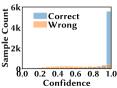
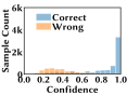
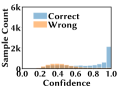
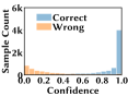
Figure 10: Histograms of prediction confidences for ResNet-50 on CIFAR-100 OOD dataset. (a) Un-calibrated. (b) Temperature scaling. (c) Scaling-binning. (d) Dirichlet calibration. (e) CCAC.

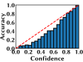
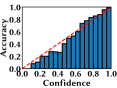
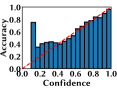
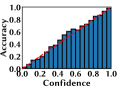
Figure 11: Reliability diagrams of prediction confidences for ResNet-50 on CIFAR-100 OOD dataset. (a) Un-calibrated. (b) Temperature scaling. (c) Scaling-binning. (d) Dirichlet calibration. (e) CCAC.

4.2.5 1000-class Image Classification with VGG16 DNN

Target DNN model. The target DNN model is the VGG16 for 1000-class image classification. The pre-trained weights of VGG16 model are directly downloaded from the Keras application package [8], which are trained on ImageNet 2012 training dataset [43].

Datasets. We evaluate the calibration performance on two datasets generated from ImageNet 2012 validation dataset [43], including augmented dataset D1 and one out-of-distribution dataset (OOD). We first randomly select 30k samples from ImageNet 2012 validation, and then perform augmentation operations on the selected samples via ImageDataGenerator in Tensorflow. For D1, the augment operations and parameters include rotation within $[-40,40]$ degrees, vertical/horizontal shift within $[-0.5,0.5]$, and horizontal flip. The OOD dataset includes 15k samples from ImageNet validation dataset and 15k samples from CIFAR-100 dataset serving as OOD samples. To fit for the input size of DNNs, the OOD samples from CIFAR-100 dataset are resized into $(224,224,3)$ using tf.image.resize with default parameters. The OOD samples are treated with “NULL” label, indicating not belonging to any of the 1000 classes. The inference accuracies on the two test datasets are 51% (D1) and 32% (OOD). Additionally, the 30k samples (in D1 or OOD ) are randomly split into a 10k dataset for training, a 2k validation dataset for hyperparameter tuning, and a 18k testing dataset for performance evaluation.

Table 17: VGG16 on ImageNet D1

Method	AUROC	AUPR	p.9	ECE	BS
MP	0.846	0.815	0.686	2.5%	0.160
TS	0.846	0.815	0.686	2.5%	0.160
CCAC-S	0.784	0.743	0.621	2.4%	0.189

Table 18: VGG16 on ImageNet OOD

Method	AUROC	AUPR	p.9	ECE	BS
MP	0.925	0.961	0.887	14.0%	0.124
TS	0.931	0.964	0.896	7.2%	0.102
CCAC-S	0.953	0.979	0.915	2.0%	0.083

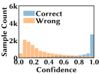
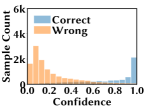
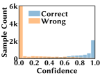
Figure 12: Histograms of prediction confidences for VGG16 on ImageNet OOD dataset. (a) Un-calibrated. (b) Temperature scaling. (c) CCAC-S.

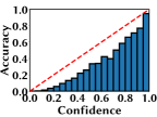
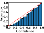
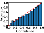
Figure 13: Reliability diagrams of prediction confidences for VGG16 on ImageNet OOD dataset. (a) Un-calibrated. (b) Temperature scaling. (c) CCAC-S.

Baselines. The ImageNet dataset contains 1000 classes, significantly increasing the trainable weights and training dataset size required in parametric calibration baselines of SB and Dirichlet. Thus, we only keep two baselines (MP and TS) for confidence calibration on ImageNet. For each dataset, the baseline TS is trained on the 10k training dataset. The 10k training dataset is the same as the one used for CCAC-S.

Our method. Given 1000 nodes in each layer, a fully-connected layer in CCAC contains more than $10^{6}$ weights for 1000-class image classification. Thus, due to limited size of D1 and OOD datasets, we only implement CCAC-S for 1000-class image classification. Specifically, the neural network of CCAC-S contains no hidden layers. The input layer contains 1000 nodes and the output layer contains 1001 nodes (including 1000 classes and one “mis-classification” class). CCAC-S is trained over 1000 epochs using the Adam optimizer (learning rate $10^{-4}$). The loss function hyperparameters ($\lambda_{1}$ and $\lambda_{2}$) and the confidence calculation method are selected with a minimal ECE on the validation dataset.

Results. The calibration results are presented in Table 18 and 18 for D1 and OOD datasets, respectively. The results show that the proposed method (CCAC-S) outperforms the baseline in terms of confidence calibration, with significant improvement on the OOD dataset. In addition, the CCAC-S offers a better mis-classification detection performance on the OOD dataset in terms of AUROC/AUPR/p.9. We further show the histograms of confidences for correct and wrong predictions in Fig. 12 on the OOD dataset. The corresponding reliability diagrams also are shown in Fig. 13 on the OOD dataset with different calibration methods.

4.2.6 1000-class Image Classification with ResNet-50 DNN

Table 19: ResNet-50 on ImageNet D1

Method	AUROC	AUPR	p.9	ECE	BS
MP	0.850	0.735	0.570	5.3%	0.154
TS	0.849	0.733	0.570	2.8%	0.152
CCAC-S	0.807	0.640	0.531	2.3%	0.171

Table 20: ResNet-50 on ImageNet OOD

Method	AUROC	AUPR	p.9	ECE	BS
MP	0.886	0.931	0.843	25.0%	0.201
TS	0.896	0.937	0.851	10.9%	0.134
CCAC-S	0.957	0.979	0.916	2.8%	0.081

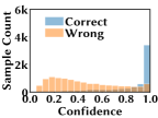
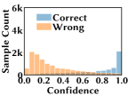
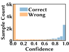
Figure 14: Histograms of prediction confidences for ResNet-50 on ImageNet OOD dataset. (a) Un-calibrated. (b) Temperature scaling. (c) CCAC-S.

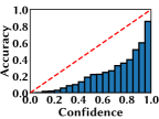
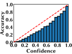
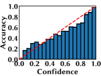
Figure 15: Reliability diagrams of prediction confidences for ResNet-50 on ImageNet OOD dataset. (a) Un-calibrated. (b) Temperature scaling. (c) CCAC-S.

Target DNN model. The target DNN model is ResNet-50 for 1000-class image classification. The pre-trained weights of target DNN model are directly downloaded from Keras application package [8], which are trained on ImageNet 2012 training dataset [43].

All the other settings, such as the datasets and architecture of the neural network in CCAC-S, are the same as those for the 1000-class VGG16 DNN described in Section 4.2.5. The inference accuracies on the two test datasets are 64% (D1) and 34% (OOD).

Results. The calibration results are presented in Table 20 and 20 for D1 and OOD datasets, respectively. The results show that the proposed method (CCAC-S) outperforms the baselines in terms of confidence calibration, with significant improvement on the OOD dataset. In addition, the CCAC-S offers a better mis-classification detection performance on OOD dataset in terms of AUROC/AUPR/p.9. We further show the histograms of confidences for correct and wrong predictions in Fig. 14 on the OOD dataset. The corresponding reliability diagrams also are shown in Fig. 15 on the OOD dataset with different calibration methods.

4.3 Results for Document Classification

We consider two document classification applications: Reuters 8-topic classification [31] and 20 Newsgroups classification [42].

4.3.1 8-topic Document Classification with DAN

Pre-processing. For the Reuters dataset, news articles are partitioned into 8 categories (R8 dataset). In our experiments, the raw documents are pre-processed with the same tokenizer and re-formatted into sequences each with 1000 words via pad_sequences, which are then used as inputs to the target DNN model.

Target DNN model. The target DNN model is a Deep Average Network (DAN), trained in TensorFlow on the R8 training dataset (5485 documents). The target DNN model includes 3 blocks with feed-forward layers, batch normalization layers, and dropout layers [21]. The DAN model is trained via Adam optimizer with a learning rate of $10^{-3}$ over 50 epochs.

Table 21: DAN on R8 D1

Method	AUROC	AUPR	p.9	ECE	BS
MP	0.885	0.484	0.236	5.3%	0.065
TS	0.884	0.470	0.238	2.9%	0.064
SB	0.938	0.691	0.410	3.2%	0.049
Dirichlet	0.816	0.338	0.150	2.8%	0.078
CCAC	0.954	0.729	0.437	1.9%	0.044
CCAC-S	0.947	0.722	0.452	2.2%	0.047
CCAC-T	-	-	-	-	-

Table 22: DAN on R8 OOD

Method	AUROC	AUPR	p.9	ECE	BS
MP	0.801	0.646	0.415	10.3%	0.171
TS	0.799	0.643	0.413	5.6%	0.180
SB	0.889	0.772	0.587	7.8%	0.129
Dirichlet	0.717	0.512	0.419	5.0%	0.192
CCAC	0.929	0.860	0.672	3.5%	0.099
CCAC-S	0.919	0.850	0.640	3.1%	0.102
CCAC-T	0.885	0.763	0.604	4.8%	0.126

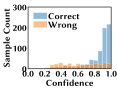
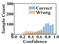
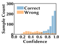
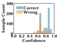
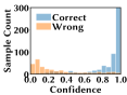
Figure 16: Histograms of prediction confidences for DAN on R8 OOD dataset. (a) Un-calibrated. (b) Temperature scaling. (c) Scaling-binning. (d) Dirichlet calibration. (e) CCAC.

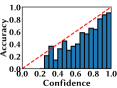
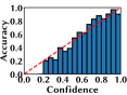
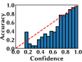
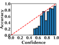
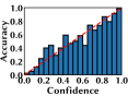
Figure 17: Reliability diagrams of prediction confidences for DAN on R8 OOD dataset. (a) Un-calibrated. (b) Temperature scaling. (c) Scaling-binning. (d) Dirichlet calibration. (e) CCAC.

Datasets. We evaluate the calibration performance on two datasets generated from the R8 dataset and Reuters-extension dataset (R52), including augmented dataset D1 and Out-of-Distribution dataset (OOD). The R52 dataset contains 1426 documents with different news topics. We first randomly select 2811 articles from R8 training dataset and 2189 articles from R8 testing dataset, and then perform augmentation operations on selected samples with the nlpaug package [33]. The augmentation operations include the OCR engine error (OcrAug) operation and the randomly typo (RandomAug) operation with substitute, swap and delete. The OOD dataset also includes 5k samples, with 1246 OOD samples from R52 dataset, 1385 samples from R8 training dataset, and 2189 samples from R8 testing datasest. As for the 1246 OOD samples from R52, the true labels are mapped to R8’s class labels. Specifically, we treat the OOD samples with label “income” and “jobs” as the “earn” category in R8, and the OOD samples with label “money-supply” as the “money-fx” category in R8. The other OOD samples from R52 are treated with the “NULL” label, indicating not belonging to any of the 8 categories in R8. The inference accuracies on two test datasets are 90% (D1) and 69% (OOD). Additionally, the 5k samples (D1 and OOD) are randomly split into a 3k dataset for training, a 0.5k validation dataset for hyperparameter tuning, and a 1.5k testing dataset for performance evaluation.

Baselines. For each dataset, the baselines of TS, SB, and Dirichlet calibration are trained on the respective 3k training dataset. For Dirichlet calibration, the regularization hyperparameters are tuned with a minimal ECE on the 0.5k validation dataset. The 3k training and 0.5k validation dataset are the same as those used for training CCAC and CCAC-S.

Our method. The neural network of CCAC is implemented with 2 hidden layers, including 10 neurons in each hidden layer. The input layer contains 8 nodes and the output layer contains 9 nodes (including 8 classes and one “mis-classification” class). CCAC is trained over 1500 epochs using the Adam optimizer (learning rate $0.002$). The loss function hyperparameters ($\lambda_{1}$ and $\lambda_{2}$) and the confidence calculation method are selected with a minimal ECE on the validation dataset. For CCAC-S, the neural network is implemented with one hidden layer, including 20 hidden nodes. The output layer of CCAC-S contains only one node, representing the “mis-classification” class. Also, the temperature scaling layer is implemented with a self-defined Keras layer with one learnable weight $T$. The CCAC-S is trained over 1500 epochs via Adam optimizer with a learning rate of $0.005$. For the transferred model CCAC-T, we first pre-train CCAC-S on dataset D1. Then, when applied to another target dataset, a set of 320 samples are randomly selected from the 3k training dataset for model transfer. In addition, we select another 200 samples from the 0.5k training dataset to tune the corresponding hyperparameters and confidence calculation method in CCAC-T.

Results. The calibration results are presented in Table 22, 22 for D1 and OOD datasets, respectively. Like for image classification applications, the results show that the proposed methods (CCAC and CCAC-S) outperform the baselines in terms of both mis-classification detection and confidence calibration, with more significant improvement on the OOD dataset. In addition, even though the CCAC-T model is transferred to the OOD dataset with fewer training samples than the baselines, it still offers a better calibration performance than baselines in terms of ECE and BS. We further show the histograms of confidences for correct and wrong predictions in Fig. 16 on the OOD dataset. The corresponding reliability diagrams also are shown in Fig. 17 on the OOD dataset with different calibration methods.

4.3.2 20-topic Document Classification with DAN

Pre-processing. The 20 Newsgroups dataset includes approximately 20k documents, which are partitioned into 20 different categories [42]. We use the 20 Newsgroups dataset provided by scikit-learn [38], including 11314 documents in the training dataset and 7532 documents in the testing dataset. In our experiment, we only use 18 categories from the 20 Newsgroups dataset, excluding category “comp.sys.mac.hardware” and category “rec.sport.hockey”. We denote the selected 18-category Newsgroups group dataset as NG18 and the remaining 2 categories as dataset NG2. The samples in NG2 will be treated as OOD samples for the target DNN model. The raw documents are pre-processed with tokenizer and re-formatted into sequences each with 1000 words via pad_sequences, which are then used inputs to the target DNN model.

Target DNN model. The target DNN model is a Deep Average Network (DAN), trained in TensorFlow on the NG18 training dataset with 18 categories (10136 documents). The target DNN model includes a pre-trained embedding layer downloaded from glove.6B [39], 3 convolution layers and 2 fully connected layers. The target DNN model is trained via Adam optimizer with a learning rate of $10^{-3}$ over 50 epochs.

Datasets. We evaluate the calibration performance on two datasets generated from the 20 Newsgroups Dataset and Reuters-8 datasets (R8), including augmented dataset D1 and Out-of-Distribution dataset (OOD). We first randomly select 3252 documents from the NG18 training dataset and 6748 documents from NG18 testing dataset, and then perform augmentation operations on the selected samples with nlpaug [33]. The augmentation operations include the OCR engine error (OcrAug) operation and the randomly typo (RandomAug) operation with substitute,swap and delete actions. The OOD dataset also includes 10k samples, with 2553 documents randomly selected from the NG18 training dataset, 1962 documents from NG2 dataset, and 5485 documents from R8 dataset. Here, both documents in NG2 and R8 are considered as OOD samples. As for the OOD samples, the true labels are mapped to NG18’s class labels. Specifically, we consider the OOD samples from NG2 with label “comp.sys.mac.hardware” as class “comp.sys.ibm.pc.hardware” and “rec.sport.hockey” as class “rec.sport.baseball” in NG18 dataset. The other OOD samples from R8 are treated with the “NULL” label, indicating not belonging to any of the categories in NG18. The inference accuracies on the two test datasets are 75% (D1) and 33% (OOD). Additionally, the 10k samples (D1 and OOD) are randomly split into a 6k dataset for CCAC training, a 1k validation dataset for hyperparameter tuning, and a 3k testing dataset for performance evaluation.

Our method. The neural network of CCAC is implemented with one hidden layer, including 20 hidden neurons. The input layer contains 18 nodes and the output layer contains 19 nodes (including 18 classes and one “mis-classification” class). CCAC is trained for 2000 epochs using the Adam optimizer (learning rate $10^{-4}$). The loss function hyperparameters ($\lambda_{1}$ and $\lambda_{2}$) and the confidence calculation method are selected with a minimal ECE on the validation dataset. For CCAC-S, the neural network is implemented with the same structure as CCAC, but the output layer contains only one node, representing the “mis-classification” class. The temperature scaling layer is implemented with a self-defined customer Keras layer with one learnable weight $T$. CCAC-S is trained over 1000 epochs using the Adam optimizer (learning rate $10^{-3}$). For the transferred model CCAC-T, we first pre-train CCAC-S on dataset D1. Then, when applied to OOD dataset, a set of 320 samples is randomly selected from the 6k training dataset for model transfer. In addition, we select another 200 samples from the 1k validation dataset to tune the corresponding hyperparameters and confidence calculation method in CCAC-T.

Table 23: DAN on 20 Newsgroups D1

Method	AUROC	AUPR	p.9	ECE	BS
MP	0.826	0.580	0.403	17.4%	0.183
TS	0.828	0.585	0.402	4.7%	0.139
SB	0.825	0.578	0.398	4.3%	0.140
Dirichlet	0.839	0.615	0.408	4.7%	0.136
CCAC	0.865	0.642	0.455	2.4%	0.125
CCAC-S	0.849	0.606	0.446	2.8%	0.133
CCAC-T	-	-	-	-	-

Table 24: DAN on 20 Newsgroups OOD

Method	AUROC	AUPR	p.9	ECE	BS
MP	0.828	0.900	0.798	40.7%	0.349
TS	0.855	0.917	0.815	7.5%	0.150
SB	0.850	0.892	0.834	7.1%	0.140
Dirichlet	0.704	0.833	0.695	8.6%	0.206
CCAC	0.861	0.894	0.875	3.9%	0.116
CCAC-S	0.910	0.933	0.906	3.0%	0.096
CCAC-T	0.865	0.895	0.873	4.7%	0.118

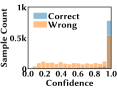
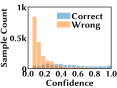
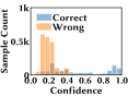
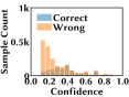
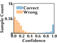
Figure 18: Histograms of prediction confidences for DAN on 20 Newsgroups OOD dataset. (a) Un-calibrated. (b) Temperature scaling. (c) Scaling-binning. (d) Dirichlet calibration. (e) CCAC.

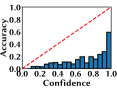
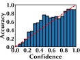
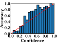
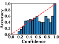
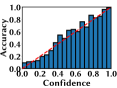
Figure 19: Reliability diagrams of prediction confidences for DAN on 20 Newsgroups OOD dataset. (a) Un-calibrated. (b) Temperature scaling. (c) Scaling-binning. (d) Dirichlet calibration. (e) CCAC.

Results. The calibration results are presented in Tables 24 and 24 for D1 and AD datasets, respectively. The results show that the proposed methods (CCAC, CCAC-S) outperform the baselines in terms of both mis-classification detection and confidence calibration, with more significant improvement on the OOD dataset. In addition, even though CCAC-T model is transferred to OOD dataset with fewer training samples than the baselines, it still offers a better calibration performance in terms of ECE and BS. We further show the histograms of confidences for correct and wrong predictions in Fig. 18 on OOD dataset. The corresponding reliability diagrams also are shown in Fig. 19 on the OOD dataset with different calibration methods.

5 Conclusion

In this paper, we propose a new post-hoc confidence calibration method, called CCAC, for DNN classifiers on OOD datasets. Building on top of a lightweight neural network, CCAC only needs the target DNN’s logit layer as input and maps it to a new calibrated confidence. The key novelty of CCAC is an auxiliary class in the calibration model to separate mis-classified samples from correctly classified ones, thus effectively mitigating the target DNN’s being confidently wrong. We also propose a simplified version of CCAC to reduce free parameters and facilitate transfer to a new unseen dataset. Our experiments on different DNN models, datasets and applications show that CCAC can consistently outperform the prior post-hoc calibration methods.

References

- [1] Martín Abadi, Ashish Agarwal, Paul Barham, Eugene Brevdo, Zhifeng Chen, Craig Citro, Greg S Corrado, Andy Davis, Jeffrey Dean, and Matthieu Devin. Tensorflow: Large-scale machine learning on heterogeneous distributed systems. arXiv preprint arXiv:1603.04467, 2016.
- [2] Vahdat Abdelzad, Krzysztof Czarnecki, Rick Salay, Taylor Denounden, Sachin Vernekar, and Buu Phan. Detecting out-of-distribution inputs in deep neural networks using an early-layer output. arXiv preprint arXiv:1910.10307, 2019.
- [3] Mohammed Al-Qizwini, Iman Barjasteh, Hothaifa Al-Qassab, and Hayder Radha. Deep learning algorithm for autonomous driving using googlenet. In IVS, 2017.
- [4] Glenn W Brier. Verification of forecasts expressed in terms of probability. Monthly weather review, 1950.
- [5] Rich Caruana, Yin Lou, Johannes Gehrke, Paul Koch, Marc Sturm, and Noemie Elhadad. Intelligible models for healthcare: Predicting pneumonia risk and hospital 30-day readmission. In KDD, 2015.
- [6] Tong Che, Xiaofeng Liu, Site Li, Yubin Ge, Ruixiang Zhang, Caiming Xiong, and Yoshua Bengio. Deep verifier networks: Verification of deep discriminative models with deep generative models. In ICML, 2020.
- [7] Chenyaofo. Pretrained models on CIFAR10/100 in pytorch. https://github.com/chenyaofo/CIFAR-pretrained-models, 2018.
- [8] François Chollet. Keras. https://keras.io, 2015.
- [9] Corinna Cortes, Giulia DeSalvo, and Mehryar Mohri. Boosting with abstention. In NIPS. 2016.
- [10] Corinna Cortes, Giulia DeSalvo, and Mehryar Mohri. Learning with rejection. In Algorithmic Learning Theory, 2016.
- [11] Jia Deng, Wei Dong, Richard Socher, Li-Jia Li, Kai Li, and Li Fei-Fei. Imagenet: A large-scale hierarchical image database. In CVPR, 2009.
- [12] Li Deng and Yang Liu. Deep Learning in Natural Language Processing. Springer, 2018.
- [13] Yarin Gal and Zoubin Ghahramani. Dropout as a bayesian approximation: Representing model uncertainty in deep learning. In ICML, 2016.
- [14] Yonatan Geifman and Ran El-Yaniv. Selective classification for deep neural networks. In NIPS. 2017.
- [15] Geifmany. VGG16 models for CIFAR-10 and CIFAR-100. https://github.com/geifmany/cifar-vgg, 2018.
- [16] Ian Goodfellow, Yoshua Bengio, and Aaron Courville. Deep Learning. MIT Press, 2016. http://www.deeplearningbook.org.
- [17] Ian J Goodfellow, Jonathon Shlens, and Christian Szegedy. Explaining and harnessing adversarial examples. 2015.
- [18] Chuan Guo, Geoff Pleiss, Yu Sun, and Kilian Q Weinberger. On calibration of modern neural networks. In ICML, 2017.
- [19] Awni Hannun, Carl Case, Jared Casper, Bryan Catanzaro, Greg Diamos, Erich Elsen, Ryan Prenger, Sanjeev Satheesh, Shubho Sengupta, and Adam Coates. Deep speech: Scaling up end-to-end speech recognition. arXiv preprint arXiv:1412.5567, 2014.
- [20] Dan Hendrycks and Kevin Gimpel. A baseline for detecting misclassified and out-of-distribution examples in neural networks. In ICLR, 2017.
- [21] Mohit Iyyer, Varun Manjunatha, Jordan Boyd-Graber, and Hal Daumé III. Deep unordered composition rivals syntactic methods for text classification. In AACL-IJCNLP, 2015.
- [22] Pavel Izmailov, Dmitrii Podoprikhin, Timur Garipov, Dmitry Vetrov, and Andrew Gordon Wilson. Averaging weights leads to wider optima and better generalization. In UAI, 2018.
- [23] Heinrich Jiang, Been Kim, Melody Guan, and Maya Gupta. To trust or not to trust a classifier. In NIPS, 2018.
- [24] Alex Kendall and Yarin Gal. What uncertainties do we need in bayesian deep learning for computer vision? In NIPS. 2017.
- [25] Alex Krizhevsky. Learning multiple layers of features from tiny images. 2009.
- [26] Meelis Kull, Miquel Perello Nieto, Markus Kängsepp, Telmo Silva Filho, Hao Song, and Peter Flach. Beyond temperature scaling: Obtaining well-calibrated multi-class probabilities with dirichlet calibration. In NIPS, 2019.
- [27] Meelis Kull, Telmo M Silva Filho, and Peter Flach. Beyond sigmoids: How to obtain well-calibrated probabilities from binary classifiers with beta calibration. Electronic Journal of Statistics, 2017.
- [28] Ananya Kumar, Percy S Liang, and Tengyu Ma. Verified uncertainty calibration. In NIPS, 2019.
- [29] Balaji Lakshminarayanan, Alexander Pritzel, and Charles Blundell. Simple and scalable predictive uncertainty estimation using deep ensembles. In NIPS, 2017.
- [30] Kimin Lee, Kibok Lee, Honglak Lee, and Jinwoo Shin. A simple unified framework for detecting out-of-distribution samples and adversarial attacks. In NIPS, 2018.
- [31] David Lewis. Reuters-21578 text categorization collection data set. https://archive.ics.uci.edu/ml/datasets/Reuters-21578+Text+Categorization+Collection.
- [32] Shiyu Liang, Yixuan Li, and Rayadurgam Srikant. Enhancing the reliability of out-of-distribution image detection in neural networks. In ICLR, 2018.
- [33] Edward Ma. NLP augmentation. https://github.com/makcedward/nlpaug, 2019.
- [34] Laurens van der Maaten and Geoffrey Hinton. Visualizing data using t-sne. Journal of Machine Learning Research, 2008.
- [35] Andrey Malinin and Mark Gales. Predictive uncertainty estimation via prior networks. In NIPS, 2018.
- [36] Sina Mohseni, Mandar Pitale, JBS Yadawa, and Zhangyang Wang. A baseline for detecting misclassified and out-of-distribution examples in neural networks. In AAAI, 2020.
- [37] Mahdi Pakdaman Naeini, Gregory Cooper, and Milos Hauskrecht. Obtaining well calibrated probabilities using bayesian binning. In AAAI, 2015.
- [38] F. Pedregosa, G. Varoquaux, A. Gramfort, V. Michel, B. Thirion, O. Grisel, M. Blondel, P. Prettenhofer, R. Weiss, V. Dubourg, J. Vanderplas, A. Passos, D. Cournapeau, M. Brucher, M. Perrot, and E. Duchesnay. Scikit-learn: Machine learning in Python. Journal of Machine Learning Research, 2011.
- [39] Jeffrey Pennington, Richard Socher, and Christopher D Manning. Glove: Global vectors for word representation. In EMNLP, 2014.
- [40] JC Platt. Probabilities for sv machines, advances in large margin classifiers, 1999.
- [41] Jonas Rauber, Wieland Brendel, and Matthias Bethge. Foolbox: A python toolbox to benchmark the robustness of machine learning models. In ICML, 2017.
- [42] Jason Rennie and Ken Lang. 20 Newsgroups Dataset. http://qwone.com/~jason/20Newsgroups.
- [43] Olga Russakovsky, Jia Deng, Hao Su, Jonathan Krause, Sanjeev Satheesh, Sean Ma, Zhiheng Huang, Andrej Karpathy, Aditya Khosla, Michael Bernstein, Alexander C. Berg, and Li Fei-Fei. ImageNet Large Scale Visual Recognition Challenge. International Journal of Computer Vision, 2015.
- [44] Jörg Sander, Bob D de Vos, Jelmer M Wolterink, and Ivana Išgum. Towards increased trustworthiness of deep learning segmentation methods on cardiac mri. In Medical Imaging 2019: Image Processing, 2019.
- [45] Peter Schulam and Suchi Saria. Can you trust this prediction? auditing pointwise reliability after learning. In AISTATS, 2019.
- [46] Jasper Snoek, Yaniv Ovadia, Emily Fertig, Ren, et al. Can you trust your model’s uncertainty? Evaluating predictive uncertainty under dataset shift. In NeurIPS, 2019.
- [47] Bianca Zadrozny and Charles Elkan. Obtaining calibrated probability estimates from decision trees and naive bayesian classifiers. In ICML, 2001.
- [48] Bianca Zadrozny and Charles Elkan. Transforming classifier scores into accurate multiclass probability estimates. In KDD, 2002.