A two-level shifted Laplace Preconditioner for Helmholtz Problems: Field-of-values analysis and wavenumber-independent convergence

Abstract

One of the main tools for solving linear systems arising from the discretization of the Helmholtz equation is the shifted Laplace preconditioner, which results from the discretization of a perturbed Helmholtz problem $-\Delta u-(k^{2}+i\varepsilon)u=f$ where $0\neq\varepsilon\in\mathbb{R}$ is an absorption parameter. In this work we revisit the idea of combining the shifted Laplace preconditioner with two-level deflation and apply it to Helmholtz problems discretized with linear finite elements. We use the convergence theory of GMRES based on the field of values to prove that GMRES applied to the two-level preconditioned system with a shift parameter $\varepsilon\sim k^{2}$ converges in a number of iterations independent of the wavenumber $k$, provided that the coarse mesh size $H$ satisfies a condition of the form $Hk^{2}\leq C$ for some constant $C$ depending on the domain but independent of the wavenumber $k$. This behaviour is sharply different to the standalone shifted Laplacian, for which wavenumber-independent GMRES convergence has been established only under the condition that $\varepsilon\sim k$ by [M.J. Gander, I.G. Graham and E.A. Spence, Numer. Math., 131 (2015), 567-614]. Finally, we present numerical evidence that wavenumber-independent convergence of GMRES also holds for pollution-free meshes, where the coarse mesh size satisfies $Hk^{3/2}\leq C$, and inexact coarse grid solves.

1 Introduction

In this work we study the solution of linear systems of equations arising from the discretization of the Helmholtz equation. We concentrate here on the interior Helmholtz problem with impedance boundary conditions, which for a domain $\Omega\subset\mathbb{R}^{d}$ with boundary $\Gamma$, $k\in\mathbb{R}$, $f_{1}\in L^{2}(\Omega)$ and $f_{2}\in L^{2}(\Gamma)$ is defined as:

(1) $$\left\{\begin{array}[]{rc}-\Delta u-k^{2}u&=f_{1}\,\,\text{ in $\Omega$,}\\ \partial_{n}u-iku&=f_{2}\,\,\text{ in $\Gamma$}.\end{array}\right.$$

The solution of these systems of equations is one of the main computational bottlenecks for solving inverse problems in various applications, e.g., in exploration geophysics and medical imaging. The standard variational formulation of (1) and its corresponding Galerkin discretization with P1 finite elements on a simplicial mesh $T_{h}$ of the domain $\Omega$ leads to a linear system

(2) $$\mathbf{A}\mathbf{u}=\mathbf{f},$$

where $\mathbf{A}\in\mathbb{C}^{N_{h}\times N_{h}}$, and $\mathbf{u},\mathbf{f}\in\mathbb{C}^{N_{h}\times N_{h}}$. Due to the oscillatory character of the solutions, in order to obtain an accurate approximation the number of gridpoints in one dimension should be at least proportional to $k$, leading to linear systems of size $N_{h}\sim k^{d}$ where $d$ is the spatial dimension. However, the Galerkin solutions are affected by the pollution effect [1, 33] and this rule is not sufficient to mantain accuracy when using discretizations with low-order finite elements for large wavenumbers. In this case the number of points in one-dimension should be chosen proportional to $k^{3/2}$ leading to very large linear systems of size $N_{h}\sim k^{3d/2}$. Moreover, the matrix $\mathbf{A}$ is non-Hermitian and indefinite, making the efficient solution of (2) with standard iterative techniques a huge challenge; for a survey see [18].

The development of fast solvers for the Helmholtz equation has been an active research area over the last decades. Notable works include the wave-ray method [4, 40], methods based on domain decomposition, and sweeping-type preconditioners [10, 11, 53] , see, e.g., the survey papers [12, 18, 22] for more references.

A very fruitful idea introduced in the landmark paper [16] is to precondition (2) with the discretization of a Helmholtz problem with absorption (or shifted Laplace problem) of the form

(3) $$\left\{\begin{array}[]{rc}-\Delta u-(k^{2}+i\varepsilon)u&=f_{1}\,\,\text{ in $\Omega$,}\\ \partial_{n}u-iku&=f_{2}\,\,\text{ in $\Gamma$},\end{array}\right.$$

where $\varepsilon$ is a real positive parameter. After discretization of (3) one obtains a linear system with coefficient matrix $\mathbf{A}_{\varepsilon}$. The complex shift $i\varepsilon$ in (3) reduces the oscillations in the solutions and allows the preconditioner $\mathbf{A}_{\varepsilon}$ to be inverted with fast methods, e.g. multigrid or domain decomposition. This preconditioner is known as the complex shifted Laplacian (CSL) or shifted Laplace preconditioner, and is a building block for several state-of-the-art solvers for the Helmholtz equation, see, e.g., the book [37] for a recent overview of extensions and industrial applications of Helmholtz solvers based on the shifted Laplacian. The resulting preconditioned system

$$\mathbf{A}\mathbf{A}_{\varepsilon}^{-1}\mathbf{g}=\mathbf{f},\,\,\mathbf{u}=\mathbf{A}_{\varepsilon}^{-1}\mathbf{g}$$

can be solved more efficiently than the original system with Krylov subspace methods for non-Hermitian systems. Here we only consider the solution of the linear system with the GMRES method. In practice, the preconditioner is inverted approximately with a fast method; denoting this approximation by $\mathbf{D}_{\varepsilon}^{-1}\approx\mathbf{A}_{\varepsilon}^{-1}$, the linear system to be analyzed is

(4) $$\mathbf{A}\mathbf{D}_{\varepsilon}^{-1}\mathbf{g}=\mathbf{f},\,\,\mathbf{u}=\mathbf{D}_{\varepsilon}^{-1}\mathbf{g}.$$

Naturally there is a tradeoff in the choice of the shift $\varepsilon$, since a small shift leads to faster convergence of the Krylov solver but only a large enough shift will allow the (approximate) inversion of $\mathbf{A}_{\varepsilon}$ with fast methods. To date, the most rigorous analysis on how to choose the shift has appeared in [21], and the series of papers [7, 25, 26]. The authors of [21] propose to separate the analysis of the shifted Laplacian in two questions:

1. Assuming that $\mathbf{A}_{\varepsilon}$ is inverted exactly, determine conditions on $\varepsilon$ for $\mathbf{A}_{\varepsilon}$ to be a good preconditioner for $\mathbf{A}$.

2. Determine conditions on $\varepsilon$ for $\mathbf{D}_{\varepsilon}^{-1}$ to be a good approximation for $\mathbf{A}_{\varepsilon}^{-1}$, in particular when using multigrid or domain decomposition methods.

More rigorously, one can use the identity

$$\mathbf{I}-\mathbf{A}\mathbf{D}_{\varepsilon}^{-1}=\mathbf{I}-\mathbf{A}_{\varepsilon}\mathbf{D}_{\varepsilon}^{-1}+\mathbf{A}_{\varepsilon}\mathbf{D}_{\varepsilon}^{-1}(\mathbf{I}-\mathbf{A}\mathbf{A}_{\varepsilon}^{-1}),$$

to show that if both $\|\mathbf{I}-\mathbf{A}_{\varepsilon}\mathbf{D}_{\varepsilon}^{-1}\|$ and $\|\mathbf{I}-\mathbf{A}\mathbf{A}_{\varepsilon}^{-1}\|$ are small (i.e., the quantitative version of statements (a) and (b)) then GMRES applied to (4), is expected to converge fast.

Some of the early works on the shifted Laplacian [52, 16, 15] focused on answering question (a) using the GMRES residual bounds based on the spectrum of the matrix. In these papers the choice $\varepsilon=\beta k^{2}$ with $\beta\in[0.5,1]$ was recommended, based on an analysis of the spectrum of the preconditioned (continuous) Helmholtz operator with Dirichlet boundary conditions in 1D in [12] and the spectrum of more general preconditioned discrete Helmholtz operators in [52]. Likewise, a combination of questions (a) and (b) was investigated in [8] using Local Fourier Analysis, leading to an expression for the near-optimal value (for guaranteed multigrid V-cycle convergence and a near-optimal minimum number of GMRES iterations) depending on the wavenumber and gridsize. For more references on how to choose the shift in the CSL preconditioner see [21, Section 1.1].

The analysis of GMRES convergence based on the distribution of the eigenvalues of the preconditioned matrix rests on the assumption that the condition number of the matrix of eigenvectors of the preconditioned matrix is small. However, this factor is hard to estimate and for some problems it can be so large that the bound may not be informative at all. Moreover, it is known that the convergence of GMRES applied to a non-normal linear system cannot be predicted only by the spectrum of the matrix [27, 38]. The authors of [21] use instead the convergence theory of GMRES based on the field of values (which we summarize in section 3.) to study question (a) above. Their main result shows that under some natural assumptions on the geometry of the domain the condition $\varepsilon\lesssim k$ (i.e., $\varepsilon\leq Ck$ with a small enough constant $C$) is sufficient for the field of values of $\mathbf{A}\mathbf{A}_{\varepsilon}^{-1}$ to be bounded away from the origin as $k\to\infty$, and therefore under this condition the number of iterations of GMRES applied to the preconditioned system remains constant as $k$ is increased.

Question (b) has been studied in [7] for general 2D and 3D problems in the context of the multigrid method. There it is shown that choosing a shift $\varepsilon\sim k^{2}$ is a necessary and sufficient condition for the convergence of multigrid with a fixed number of (weighted Jacobi) smoothing steps applied to a linear system with coefficient matrix $\mathbf{A}_{\varepsilon}$. Regarding domain decomposition methods and question (b), the work [25] investigates the requirements for an additive Schwarz preconditioner $\mathbf{D}_{\varepsilon}^{-1}\approx\mathbf{A}_{\varepsilon}^{-1}$ (with Dirichlet transmission conditions between subdomains and coarse grid correction) to be effective as a preconditioner for a problem with coefficient matrix $\mathbf{A}_{\varepsilon}$, i.e., to obtain fast convergence of GMRES applied to a linear system with coefficient matrix $\mathbf{A}_{\varepsilon}\mathbf{D}_{\varepsilon}^{-1}$. There it is concluded that a sufficient condition is $\varepsilon\lesssim k^{2}$. The more recent paper [26] introduces an additive Schwarz method with local impedance boundary conditions as transmission conditions between subdomains and shows that it is possible to obtain wavenumber independent convergence also under the condition $\varepsilon\sim k^{1+\beta}$ for $\beta$ arbitrarily small. Together, these recent results imply that there exists a rigorously quantified gap between the condition for having a good preconditioner (which requires a small shift $\varepsilon\lesssim k$) and the requirement for being able to (approximately) invert $\mathbf{A}_{\varepsilon}$ (for which $\varepsilon\sim k^{2}$ or at least $\varepsilon\sim k^{1+\beta}$ with $\beta>0$ arbitrarily small is necesary), thus motivating the need for more advanced preconditioning techniques.

In this paper we revisit the combination of the shifted Laplacian with two-level deflation, which was introduced in [48, 47] based on previous work in [14], see also [24] for an analysis of the method proposed in [14]. We extend the simplified variant of two-level deflation from [48, 47] to Helmholtz problems discretized with finite elements, and we contribute to the line of analysis proposed in [21] by studying the analogous of question (a) for the two-level shifted Laplacian combined with deflation. We use the framework for the analysis of two-level preconditioners from [29].

The method that we use combines the shifted Laplacian with a projection-based preconditioner which removes the components of $\mathbf{A}\mathbf{A}_{\varepsilon}^{-1}$ that cause the slow convergence of a Krylov subspace method applied to the linear sytem. Algebraically this idea can be motivated as follows. Let $\mathbf{Q}\in\mathbb{C}^{n\times n}$ be a projection operator, i.e., a matrix such that $\mathbf{Q}^{2}=\mathbf{Q}$. If ${\mathcal{R}}(\mathbf{Q})$ is the range of $\mathbf{Q}$ and ${\mathcal{N}}(\mathbf{Q})$ its nullspace, the direct sum decomposition $\mathbb{C}^{n}={\mathcal{R}}(\mathbf{Q})\oplus{\mathcal{N}}(\mathbf{Q})$ holds and $\mathbf{A}^{-1}$ can be split as

$$\mathbf{A}^{-1}=\mathbf{A}^{-1}(\mathbf{I}-\mathbf{Q})+\mathbf{A}^{-1}\mathbf{Q},$$

note that $(\mathbf{I}-\mathbf{Q})$ is also a projection. Therefore, a sensible approximation for the inverse of $\mathbf{A}$ is

(5) $$\mathbf{B}=\mathbf{A}_{\varepsilon}^{-1}(\mathbf{I}-\mathbf{Q})+\mathbf{A}^{-1}\mathbf{Q}.$$

The crucial point is that the projection can be chosen so that the term $\mathbf{A}^{-1}\mathbf{Q}$ on the right can be computed cheaply by solving a smaller linear system. If $m<n$ and $\mathcal{U}$ is an subspace of $\mathbb{C}^{n}$ spanned by the columns of a full rank matrix $\mathbf{U}\in\mathbb{C}^{n\times m}$ such that $\mathbf{U}^{\ast}\mathbf{A}\mathbf{U}$ is nonsingular (where the superscript $*$ denotes the conjugate transpose), the projection $\mathbf{Q}$ with ${\mathcal{R}}(\mathbf{Q})=\mathbf{A}\mathcal{U}$ and ${\mathcal{N}}(\mathbf{Q})=\mathcal{U}^{\perp}$ (the orthogonal complement of $\mathcal{U}$ in the Euclidean inner product) has the form

$$\mathbf{Q}=\mathbf{A}\mathbf{U}(\mathbf{U}^{*}\mathbf{A}\mathbf{U})^{-1}\mathbf{U}^{*},$$

which gives

(6) $$\mathbf{B}=\mathbf{A}_{\varepsilon}^{-1}(\mathbf{I}-\mathbf{A}\mathbf{U}(\mathbf{U}^{*}\mathbf{A}\mathbf{U})^{-1}\mathbf{U}^{*})+\mathbf{U}(\mathbf{U}^{*}\mathbf{A}\mathbf{U})^{-1}\mathbf{U}^{*}$$

and the term $\mathbf{U}(\mathbf{U}^{*}\mathbf{A}\mathbf{U})^{-1}\mathbf{U}^{*}$ can be computed by inverting a smaller system with coefficient matrix $\mathbf{U}^{*}\mathbf{A}\mathbf{U}$. It follows easily using this projection representation that if $\mathbf{B}$ is used as a preconditioner for $\mathbf{A}$ then $\mathbf{A}\mathbf{B}$ equals the identity when restricted to the subspace $\mathcal{U}$, so the spectrum of the preconditioned matrix $\mathbf{A}\mathbf{B}$ contains one as an eigenvalue with multiplicity (at least) $m=\mathrm{dim}(\mathcal{U})$. Moreover, if the subspace $\mathcal{U}$ contains the solution $\mathbf{u}$ we have $\mathbf{f}=\mathbf{A}\mathbf{u}\in\mathbf{A}\mathcal{U}$, and GMRES applied to the preconditioned linear system $\mathbf{A}\mathbf{B}\mathbf{u}=\mathbf{f}$ with a zero initial guess will converge in one step. Projection-based preconditioners of the form (6) are related to classical deflation methods in which a projection operator is used to remove near-singular eigenspaces responsible for slowing down the convergence of a Krylov subspace iteration, the main difference being that in classical deflation the resulting deflated linear system is singular, i.e., the eigenvalues are shifted to zero, not to one. For more on the connection between two-level methods, projections and deflation see [23].

An important class of methods that lead to preconditioners of the form (6) are two-level (or two-grid) methods, which are the basis of the multigrid method [51]. In [48, 47], the authors consider a finite difference discretization of the problem on a grid $G_{h}$ and a coarse grid $G_{H}\subset G_{h}$, and choose the subspace $\mathcal{U}$ as the span of the columns of (the matrix representation of) the two-grid prolongation operator $\mathbf{P}$. Here we analyze an extension of this preconditioner to the finite element setting, where the mesh $T_{h}$ is coarsened by choosing a mesh $T_{H}$ such that the elements in $T_{H}$ are unions of elements of $T_{h}$. If $\mathcal{V}_{h},\mathcal{V}_{H}$ are spaces of P1 finite elements to $T_{h}$ and $T_{H}$ respectively, we then have $\mathcal{V}_{H}\subset\mathcal{V}_{h}$ and the prolongation operator is defined trivially by this inclusion. The resulting preconditioner is (see section 4. for more details)

$$\mathbf{B}_{\varepsilon}=\mathbf{A}_{\varepsilon}^{-1}(\mathbf{I}-\mathbf{A}\mathbf{P}\mathbf{A}_{H}^{-1}\mathbf{P}^{*})+\mathbf{P}\mathbf{A}_{H}^{-1}\mathbf{P}^{*},$$

leading to the preconditioned system

$$\mathbf{A}\mathbf{B}_{\varepsilon}\mathbf{g}=\mathbf{f}.$$

The main result in our paper is Theorem 3.1, where we prove that it is possible to close the gap between the requirements for $\varepsilon$, i.e., we show that wavenumber-independent GMRES convergence can be obtained with the two-level shifted Laplacian even in the case of a large shift $\varepsilon\sim k^{2}$, provided that the coarse grid size satisfies a condition of the form $Hk^{2}<C$ for some constant $C>0$ depending only on the domain $\Omega$ (but independent of the wavenumber $k$). Note that in this theorem we are assuming that the shifted Laplacian and the coarse grid system are inverted exactly.

This result also confirms what has been previously observed in the spectral analysis of a 1D model problem in [48, 37] where it has been shown (using Fourier analysis on a one-dimensional Helmholtz problem with Dirichlet boundary conditions) that when the shifted Laplacian is combined with two-level deflation with a complex shift $\varepsilon=\beta k^{2}$ it is possible to increase $\beta$ without greatly affecting the spectrum of the preconditioned matrix.

We prove Theorem 3.1 for weighted GMRES in the inner product induced by the inverse of the domain mass matrix, and show that this norm is a natural norm to measure the residuals of the preconditioned system since it corresponds to the dual $L^{2}$ norm when $\mathbb{C}^{N_{h}}$ is identified with the space of coordinates of $\mathcal{V}_{h}^{\prime}$ (Proposition 2.4, (c)). Fortunately, for a sequence of quasi-uniform meshes one can use a scaling argument and norm equivalences to show that the result also holds for GMRES in the Euclidean inner product (Corollary 3.19, part (a)).

This paper is organized as follows: In section 2. we review some basic results on the variational formulation of Helmholtz problems, focusing on the conditions for existence and uniqueness of solutions to these problems and their stability. In sections 3. and 4. we introduce the finite element formulation of the Helmholtz and shifted Laplace problems and the convergence theory of GMRES based on the field of values. In section 5. the two-grid preconditioner is introduced and we prove our main result. Finally, in section 6. we present some numerical experiments to illustrate our results.

2 Preliminaries: A recap of the variational formulation and finite element approximation of Helmholtz problems

In this section we review some basic results on the variational formulation of Helmholtz problems, focusing on the conditions for existence and uniqueness of solutions to these problems and their stability. In the second part we discuss the finite element approximation of Helmholtz problems with the Galerkin method. We refer the reader to [49] for a very good introduction to the variational formulation of Helmholtz problems. To simplify the notation, we will write $a\lesssim b$ to denote that there exists a constant $C$ such that $a\leq Cb$ independent of the parameters on which $a$ and $b$ may depend. Moreover, we write $a\sim b$ when $a\lesssim b$ and $b\lesssim a$.

Given a complex inner product space $\mathcal{V}$ we denote its sesquilinear inner product by $(\cdot,\cdot)_{\mathcal{V}}$. The antidual space (of continuous conjugate-linear functionals from $\mathcal{V}$ to $\mathbb{C}$) is denoted by $\mathcal{V}^{{}^{\prime}}$. The duality pairing $\langle\cdot,\cdot\rangle_{\mathcal{V}^{\prime}\times\mathcal{V}}:\mathcal{V}^{\prime}\times\mathcal{V}\to\mathbb{C}$ is defined for $f\in\mathcal{V}^{\prime}$, $v\in\mathcal{V}$ as

$$\langle f,v\rangle_{\mathcal{V}^{\prime}\times\mathcal{V}}=f(v).$$

The dual norm in the space $\mathcal{V}^{{}^{\prime}}$ is defined by

$$\|f\|_{\mathcal{V}^{{}^{\prime}}}=\sup_{0\neq v\in\mathcal{V}}\frac{|\langle f,v\rangle_{\mathcal{V}^{\prime}\times\mathcal{V}}|}{\|v\|_{\mathcal{V}}}.$$

We will drop the subscripts $\mathcal{V}^{\prime},\mathcal{V}$ when this introduces no ambiguities, and write only $\langle\cdot,\cdot\rangle$ and $\|\cdot\|$. Let $\Omega\subset\mathbb{R}^{d}$ be a convex polyhedron in $\mathbb{R}^{d}$ (where $d=1,2,3$) with boundary $\Gamma$. Recall that the Sobolev space $L^{2}(\Omega)$ of square integrable functions is equipped with the inner product

$$(u,v)_{L^{2}(\Omega)}=\left(\int_{\Omega}u\overline{v}\right)^{1/2}.$$

The higher order Sobolev spaces $H^{m}(\Omega)$ consist of functions $u\in L^{2}(\Omega)$ that have weak derivatives $\partial^{\alpha}u$ in $L^{2}(\Omega)$ for all multi-indices $\alpha$ with $|\alpha|\leq m$. The standard inner product in $H^{m}(\Omega)$ is given by

$$(u,v)_{m}=\sum_{|\alpha|\leq m}(\partial^{\alpha}u,\partial^{\alpha}v)_{L^{2}(\Omega)},$$

and the induced norm is denoted by $\|\cdot\|_{m,\Omega}$. In the space $H^{m}(\Omega)$ we also introduce the seminorm

$$|u|_{m}=\sum_{|\alpha|=m}\|\partial^{\alpha}u\|_{L^{2}(\Omega)}.$$

The variational formulation of the Helmholtz problem requires the use of a special $k$-weighted inner product in the space $H^{1}(\Omega)$. Given $k\in\mathbb{R}$, we define the Helmholtz energy inner product on $H^{1}(\Omega)$ by

$$(u,v)_{k,1,\Omega}=(\nabla u,\nabla v)_{L^{2}(\Omega)}+k^{2}(u,v)_{L^{2}(\Omega)},$$

for any $u,v\in H^{1}(\Omega)$. The induced norm will be denoted by $\|\cdot\|_{1,k,\Omega}$. After multiplying each side of (1) with a test function $v\in H^{1}(\Omega)$, integrating by parts and substituting the boundary condition, the problem can be restated in the variational form

(7) $$\text{Find $u\in H^{1}(\Omega)$ such that }\,a(u,v)=\langle f,v\rangle\text{ for all }v\in H^{1}(\Omega),$$

where the sesquilinear form $a:H^{1}(\Omega)\times H^{1}(\Omega)\to\mathbb{C}$ and the antilinear functional $f:L^{2}(\Omega)\to\mathbb{C}$ are given by

(8) $$a(u,v) =\int_{\Omega}\nabla u\overline{\nabla v}-k^{2}\int_{\Omega}u\overline{v}-ik\int_{\Gamma}u\overline{v},$$

(9) $$\langle f,v\rangle =\int_{\Omega}f_{1}\overline{v}+\int_{\Gamma}f_{2}\overline{v}.$$

The following lemma summarizes some properties of the sesquilinear form of the Helmholtz problem.

Lemma 2.1.

Let $a$ be the sesquilinear form (8) of the Helmholtz problem. The following properties hold:

• [43, Lemma 8.1.6], [49, p.118] The form $a$ is continuous with continuity constant $C_{c}$ independent of $k$, i.e., there exists $C_{c}$ such that for all $u,v\in H^{1}(\Omega),k\in\mathbb{R}$:

  $$|a(u,v)|\leq C_{c}\|u\|_{1,k,\Omega}\|v\|_{1,k,\Omega}$$

• The form $a$ satisfies the Gårding inequality (as an equality)

  (10) $$\|u\|_{1,k,\Omega}^{2}=\Re a(u,u)+2k^{2}\|u\|_{L^{2}(\Omega)}^{2}.$$

It can be shown [49, Lemma 6.17] that associated to the sesquilinear form $a$ there exists a bounded operator $\mathcal{A}:H^{1}(\Omega)\to H^{1}(\Omega)^{\prime}$ such that

(11) $$a(u,v)=\langle\mathcal{A}u,v\rangle,$$

using the operator $\mathcal{A}$, the variational problem can be rewritten as

(12) $$\text{Find $u\in H^{1}(\Omega)$ such that }\mathcal{A}u=f.$$

The next theorem gives a stability estimate for the Helmholtz problem. For the definition of the norm $\|\cdot\|_{1/2,\Gamma}$ see [28, Section 6.2.4]

Theorem 2.2.

Let $\Omega\subset\mathbb{R}^{d}$ be a bounded convex domain with boundary $\Gamma$, where $d=2,3$. Given $k_{0}>0$, there exists a constant $C$ (depending only on $\Omega$) such that for any $g\in L^{2}(\Omega),h\in L^{2}(\Gamma)$ and $k>k_{0}$ the solution of the Helmholtz problem satisfies

(13) $$\|u\|_{1,k,\Omega} \leq C(\|f_{1}\|_{L^{2}(\Omega)}+\|f_{2}\|_{L^{2}(\Gamma)}).$$

Moreover, if $u\in H^{2}(\Omega)$:

(14) $$|u|_{H^{2}(\Omega)}\leq C[(1+k)(\|f_{1}\|_{L^{2}(\Omega)}+\|f_{2}\|_{L^{2}(\Gamma)})+\|f_{2}\|_{1/2,\Gamma}].$$

Proof 2.3.

See [43, Prop. 8.1.4] for the case $d=2$ and [31, Prop. 3.4, 3.6] for the case $d=3$.

2.1 Finite element approximation of Helmholtz problems

In this section we recall the Galerkin formulation of the Helmholtz problem. Let $\{T_{h}\}_{h>0}$ be a family of conforming simplicial meshes of $\Omega$, where $h=\max_{K\in T_{h}}\mathrm{diam}(K)$ denotes the mesh diameter. We assume that the family $\{T_{h}\}_{h>0}$ is shape-regular, i.e.,

$$\sup_{h>0}\max_{K\in T_{h}}\frac{\mathrm{diam}(K)}{\rho(K)}\leq C<\infty.$$

We let $\mathcal{V}_{h}$ be the space of P1 finite elements subordinate to $T_{h}$ spanned by the standard nodal basis $\Phi_{h}=(\phi_{1},\ldots,\phi_{N_{h}})$. To simplify the notation, in what follows we omit the subscripts and denote the $L^{2}$ inner product by $(\cdot,\cdot)$ and the corresponding norm by $\|\cdot\|$. Every element $u=\sum_{i=1}^{N_{h}}u_{i}\phi_{i}\in\mathcal{V}_{h}$ can be represented by the vector of coordinates $\mathbf{u}=(u_{1},\ldots,u_{N_{h}})\in\mathbb{C}^{N_{h}}$, we write this correspondence as

$$u=\Phi_{h}\mathbf{u}.$$

Associated to $\Phi_{h}$ there exists a canonical basis of antilinear functionals $\Phi^{{}^{\prime}}_{h}=(\phi_{1}^{{}^{\prime}},\ldots,\phi_{N_{h}}^{{}^{\prime}})$ for the space $\mathcal{V}_{h}^{{}^{\prime}}$, that satisfies

$$\langle\phi_{i}^{{}^{\prime}},\phi_{j}\rangle=\phi_{i}^{{}^{\prime}}(\phi_{j})=\delta_{ij},\,\text{for }\,i,j,=1,\ldots,N_{h},$$

We write $f=\Phi_{h}^{\prime}\mathbf{f}$ for the coordinate correspondence between $\mathbb{C}^{N_{h}}$ and $\mathcal{V}_{h}^{\prime}$. In this notation, we have

$$\mathbf{u}=(\langle\phi_{1}^{{}^{\prime}},u\rangle,\ldots,\langle\phi_{N_{h}}^{{}^{\prime}},u\rangle)^{*},$$

here ^∗ denotes the conjugate transpose. Recall that if $\mathbf{D}\in\mathbb{C}^{N\times N}$ is a Hermitian positive definite (HPD) matrix, the inner product $(\cdot,\cdot)_{\mathbf{D}}$ induced by $\mathbf{D}$ on $\mathbb{C}^{N}$ is defined as

$$(\mathbf{x},\mathbf{y})_{\mathbf{D}}=\mathbf{y}^{*}\mathbf{D}\mathbf{x},$$

the corresponding inner product on $\mathbb{C}^{n}$ will be denoted by $\|\cdot\|_{\mathbf{D}}$.

When $\mathbb{C}^{N_{h}}$ is identified with the coordinate space of $\mathcal{V}_{h}$ via $\Phi_{h}$, the domain mass matrix $\mathbf{M}\in\mathbb{C}^{N_{h}\times\mathbf{N}_{h}}$ defined as

(15) $$\mathbf{M}_{ij}=(\phi_{j},\phi_{i})_{L^{2}(\Omega)},\,\,1\leq i,j\leq N_{h}.$$

induces a norm in $\mathbb{C}^{N_{h}}$ corresponding to the $L^{2}$ norm in the space $\mathcal{V}_{h}$. This implies that for all $\mathbf{u},\mathbf{v}\in\mathbb{C}^{N_{h}}$ and $u=\Phi_{h}\mathbf{u},v=\Phi_{h}\mathbf{v}\in\mathcal{V}_{h}$:

$$(\mathbf{u},\mathbf{v})_{\mathbf{M}} =(u,v)_{L^{2}(\Omega)}.$$

The Riesz representation theorem implies that for every $f\in\mathcal{V}_{h}^{\prime}$ there exists a unique $u_{f}\in\mathcal{V}_{h}$ such that

$$\int_{\Omega}u_{f}\overline{v}=\langle f,v\rangle,$$

for all $v\in\mathcal{V}_{h}$. The mapping $\tau:\mathcal{V}_{h}^{\prime}\to\mathcal{V}_{h}$ defined by $\tau(f)=u_{f}$ is called the Riesz map (with respect to the $L^{2}$ inner product). The corresponding representation in $\mathbb{C}^{N_{h}}$ of the duality pairing $\langle\cdot,\cdot\rangle$, the $L^{2}$ Riesz map and the dual norm is explained in the next proposition, for completeness we include the proof from chapter 6 of [42].

Proposition 2.4.

The following statements hold:

1. The duality pairing $\langle\cdot,\cdot\rangle:\mathcal{V}_{h}^{{}^{\prime}}\times\mathcal{V}_{h}\to\mathbb{C}$ is represented by the Euclidean product in $\mathbb{C}^{N_{h}}$, that is, for $\mathbf{f},\mathbf{u}\in\mathbb{C}^{N_{h}}$, $u=\Phi_{h}\mathbf{u}$ and $f=\Phi^{{}^{\prime}}_{h}\mathbf{f}$:

   $$\langle f,u\rangle=\mathbf{u}^{*}\mathbf{f}.$$

2. The matrix representation of the $L^{2}$ Riesz map $\tau:\mathcal{V}_{h}^{\prime}\to\mathcal{V}_{h}$ is

   the inverse of the mass matrix $\mathbf{M}$:

   (16) $$\mathbf{M}^{-1}=\Phi_{h}\circ\tau\circ\Phi^{\prime}\in\mathbb{C}^{N_{h}\times N_{h}}.$$

3. The norm in $\mathbb{C}^{N_{h}}$ corresponding to the dual norm in $\mathcal{V}_{h}^{\prime}$ is the norm induced by the inverse of the mass matrix $\mathbf{M}^{-1}$ from (16), that is, for $\mathbf{f}\in\mathbb{C}^{N_{h}}$ and $f=\phi^{{}^{\prime}}\mathbf{f}$ we have:

   $$\|\mathbf{f}\|_{\mathbf{M}^{-1}}=\sup_{\mathbf{u}\in\mathbb{C}^{N_{h}}}\frac{|\mathbf{u}^{*}\mathbf{f}|}{\|\mathbf{u}\|_{\mathbf{M}}}=\sup_{u\in\mathcal{V}_{h}}\frac{|\langle f,u\rangle|}{\|u\|}.$$

Proof 2.5.

For part (a), let $\mathbf{u}=(u_{1},\ldots,\mathbf{u}_{N_{h}})$ and $\mathbf{f}=(f_{1},\ldots,\mathbf{f}_{N_{h}})$. We have

$$\langle f,u\rangle =\langle\sum_{i=1}^{N_{h}}f_{i}\phi_{i}^{\prime},\sum_{j=1}^{N_{h}}u_{j}\phi_{j}\rangle$$

$$=\sum_{i,j=1}^{N_{h}}f_{i}\overline{u}_{j}\langle\phi_{i}^{\prime},\phi_{j}\rangle=\sum_{i=1}^{N_{h}}f_{i}\overline{u}_{i}=\mathbf{u}^{*}\mathbf{f}.$$

For part (b), suppose that $\mathbf{M}_{\tau}\in\mathbb{C}^{N_{h}\times N_{h}}$ is the matrix representation of the Riesz map $\tau:\mathcal{V}_{h}^{\prime}\to\mathcal{V}_{h}$. With part (a) we obtain

$$\mathbf{u}^{*}\mathbf{f}=\langle f,u\rangle =(\tau f,u)=(\mathbf{M}_{\tau}\mathbf{f},\mathbf{u})_{\mathbf{M}}=\mathbf{u}^{*}\mathbf{M}\mathbf{M}_{\tau}\mathbf{f},\text{ for all }\mathbf{f},\mathbf{u}\in\mathbb{C}^{N_{h}},$$

which implies $\mathbf{M}\mathbf{M}_{\tau}=\mathbf{I}$, so $\mathbf{M}_{\tau}=\mathbf{M}^{-1}$. For part (c), given $\mathbf{f}\in\mathbb{C}^{N_{h}}$ the Cauchy-Schwarz inequality in the inner product induced by $\mathbf{M}^{-1}$ implies that for every $\mathbf{g}\in\mathbb{C}^{N_{h}}$:

$$|(\mathbf{f},\mathbf{g})_{\mathbf{M}^{-1}}|\leq\|\mathbf{f}\|_{\mathbf{M}^{-1}}\|\mathbf{g}\|_{\mathbf{M}^{-1}},$$

with equality when $\mathbf{g}$ is a scalar multiple of $\mathbf{f}$. Therefore,

$$\|\mathbf{f}\|_{\mathbf{M}^{-1}}=\frac{|(\mathbf{f},\mathbf{f})_{\mathbf{M}^{-1}}|}{\|\mathbf{f}\|_{\mathbf{M}^{-1}}} =\sup_{\mathbf{g}\in\mathbb{C}^{N_{h}}}\frac{|(\mathbf{f},\mathbf{g})_{\mathbf{M}^{-1}}|}{\|\mathbf{g}\|_{\mathbf{M}^{-1}}}$$

$$=\sup_{\mathbf{g}\in\mathbb{C}^{N_{h}}}\frac{|(\mathbf{M}^{-1}\mathbf{g})^{*}\mathbf{f}|}{\|\mathbf{g}\|_{\mathbf{M}^{-1}}}$$

$$=\sup_{\mathbf{u}\in\mathbb{C}^{N_{h}}}\frac{|(\mathbf{M}^{-1}\mathbf{M}\mathbf{u})^{*}\mathbf{f}|}{\|\mathbf{M}\mathbf{u}\|_{\mathbf{M}^{-1}}}$$

$$=\sup_{\mathbf{u}\in\mathbb{C}^{N_{h}}}\frac{|\mathbf{u}^{*}\mathbf{f}|}{\|\mathbf{u}\|_{\mathbf{M}}}=\sup_{u\in\mathcal{V}_{h}}\frac{|\langle f,u\rangle|}{\|u\|}.$$

The Galerkin problem in $\mathcal{V}_{h}$ takes the form

(17) $$\text{Find $u\in\mathcal{V}_{h}$ such that }\,a(u,v)=f(v)\text{ for all }v\in\mathcal{V}_{h}.$$

Using the operator $\mathcal{A}_{h}:\mathcal{V}_{h}\to\mathcal{V}_{h}^{\prime}$ defined as in (11) we see that the Galerkin problem is equivalent to finding a solution $u\in\mathcal{V}_{h}$ to the functional equation

$$\mathcal{A}_{h}u=f|_{\mathcal{V}_{h}},$$

where the right hand side is the restriction of $f$ to $\mathcal{V}_{h}$. If $u=\Phi\mathbf{u}$ and $f=\Phi^{\prime}\mathbf{f}$, we obtain the linear-algebraic formulation of the Galerkin problem

(18) $$\mathbf{A}\mathbf{u}=\mathbf{f},$$

where the matrix $\mathbf{A}\in\mathbb{C}^{N_{h}\times N_{h}}$ and the vector $\mathbf{f}\in\mathbb{C}^{N_{h}}$ are given by

$$\mathbf{A}_{ij} =a(\phi_{j},\phi_{i}),\,\,\,1\leq i,j\leq N_{h}.$$

$$\mathbf{f} =(\langle f,\phi_{1}\rangle,\ldots,\langle f,\phi_{N_{h}}\rangle)^{T}.$$

In the case of Helmholtz problems with the sesquilinear form $a$ given by (8), the matrix $\mathbf{A}$ from the linear system has the form

$$\mathbf{A}=\mathbf{S}-k^{2}\mathbf{M}-ik\mathbf{N},$$

where $\mathbf{M}$ is the mass matrix (15), and $\mathbf{S},\mathbf{N}$ are defined by

$$\mathbf{S}_{ij} =(\nabla\phi_{j},\nabla\phi_{i}),\,\,\,\mathbf{N}_{ij}=(\phi_{j},\phi_{i})_{L^{2}(\partial\Omega)},\,\,\,1\leq i,j\leq N_{h}.$$

To finish this section, we discuss the approximability properties of the space $\mathcal{V}_{h}$. We assume that $\mathcal{V}_{h}$ is a space of piecewise linear Lagrange finite elements on a simplicial mesh (triangular or tetrahedral, in 2D or 3D respectively). Under this assumption, the Scott-Zhang interpolation operator $\Pi_{SZ}:H^{1}(\Omega)\to\mathcal{V}_{h}$ is well defined (see [17, Section 1.6.2]). Using the norm equivalence

$$\|u\|_{1,k,\Omega}\sim k\|u\|_{L^{2}(\Omega)}+\|\nabla u\|_{L^{2}(\Omega)}$$

and standard interpolation estimates (see [17, Lemma 1.130]) it can be shown that the Scott-Zhang interpolation operator $\Pi_{SZ}$ has the property that for all $w\in H^{2}(\Omega)$:

(19) $$\|w-\Pi_{SZ}w\|_{1,k,\Omega}\lesssim h\|w\|_{H^{2}(\Omega)}+hk\|w\|_{H^{1}(\Omega)}$$

and for $w\in H^{1}(\Omega)$

(20) $$\|w-\Pi_{SZ}w\|_{1,k,\Omega}\lesssim(1+hk)\|w\|_{H^{1}(\Omega)}.$$

2.2 The shifted Laplace preconditioner and GMRES

Given $\varepsilon>0$, we consider the Helmholtz problem with absorption (or “shifted Laplace” problem)

(21) $$\left\{\begin{array}[]{rc}-\Delta u-(k^{2}+i\varepsilon)u&=f_{1}\,\,\text{ in $\Omega$,}\\ \partial_{n}u-iku&=f_{2}\,\,\text{ in $\Gamma$}.\end{array}\right.$$

with corresponding variational formulation

(22) $$\text{Find $u\in H^{1}(\Omega)$ such that }\,a_{\varepsilon}(u,v)=\langle f,v\rangle\text{ for all }v\in H^{1}(\Omega),$$

with the sesquilinear form $a_{\varepsilon}$ and the antilinear functional $f$ given by

(23) $$a_{\varepsilon}(u,v) =\int_{\Omega}\nabla u\overline{\nabla v}-(k^{2}+i\varepsilon)\int_{\Omega}u\overline{v}-ik\int_{\Gamma}u\overline{v}$$

(24) $$\langle f,v\rangle =\int_{\Omega}f_{1}\overline{v}+\int_{\Gamma}f_{2}\overline{v}.$$

The next theorem summarizes the properties of the sesquilinear form $a_{\varepsilon}$.

Lemma 2.6.

[21, Lemma 3.1] Let $a_{\varepsilon}$ be the sesquilinear form of the shifted Laplace problem . The following properties hold:

• The form $a_{\varepsilon}$ is continuous, that is, if $0<\varepsilon\lesssim k^{2}$ then given $k_{0}>0$ there exists a constant $C_{c}$ independent of $k,\varepsilon$ such that for all $k>k_{0}$, and $u,v\in H^{1}(\Omega)$

  $$|a_{\varepsilon}(u,v)|\leq C_{c}\|u\|_{1,k,\Omega}\|v\|_{1,k,\Omega}.$$

• The form $a_{\varepsilon}$ is coercive, that is, if $0<\varepsilon\lesssim k^{2}$ there exists a constant $\alpha>0$ independent of $k,\varepsilon$ such that for all $k>0$ and $u\in H^{1}(\Omega)$

  $$|a_{\varepsilon}(u,u)|\geq\alpha\frac{\varepsilon}{k^{2}}\|u\|_{1,k,\Omega}^{2}.$$

The matrix $\mathbf{A}_{\varepsilon}$ corresponding to the discrete shifted Laplace problem has the form

$$\mathbf{A}_{\varepsilon}=\mathbf{S}-(k^{2}+i\varepsilon)\mathbf{M}-ik\mathbf{N}=\mathbf{A}-i\varepsilon\mathbf{M}.$$

We will use in our analysis a bound for the GMRES residuals based on the field of values. Recall that given a Hermitian positive definite (HPD) matrix $\mathbf{D}\in\mathbb{C}^{N\times N}$ and an arbitrary $\mathbf{C}\in\mathbb{C}^{N\times N}$, the field of values of $\mathbf{C}$ in the inner product induced by $\mathbf{D}$ is the set

$$\mathcal{F}_{\mathbf{D}}(\mathbf{C})=\left\{\frac{(\mathbf{C}\mathbf{x},\mathbf{x})_{\mathbf{D}}}{(\mathbf{x},\mathbf{x})_{\mathbf{D}}}:\mathbf{x}\in\mathbb{C}^{N},\mathbf{x}\neq\mathbf{0}\right\}.$$

Note that the spectrum of $\mathbf{C}$ is contained in $\mathcal{F}_{\mathbf{D}}(\mathbf{C})$ for any HPD matrix $\mathbf{D}$. The Toeplitz-Hausdorff theorem states that the field of values is a convex, compact set [32], hence the following quantity is well defined:

$$\nu_{\mathbf{D}}(\mathbf{C})=\min_{z\in\mathcal{F}_{\mathbf{D}}(\mathbf{C})}|z|.$$

The next theorem by Elman [9] shows that quantities related to the field of values can be used to bound the residuals of a minimum residual method in an arbitrary inner product.

Theorem 2.7.

Let $\mathbf{r}_{0}$ be the initial residual of the GMRES method applied to the linear system

$$\mathbf{C}\mathbf{u}=\mathbf{f}$$

in the inner product induced by $\mathbf{D}$. The $n$-th residual $\mathbf{r}_{n}$ satisfies:

(25) $$\frac{\|\mathbf{r}_{n}\|_{\mathbf{D}}}{\|\mathbf{r}_{0}\|_{\mathbf{D}}}\leq\left(1-\frac{\nu_{\mathbf{D}}(\mathbf{C})^{2}}{\|\mathbf{C}\|_{\mathbf{D}}^{2}}\right)^{n/2},$$

The proof of the GMRES bound based on the field of values relies on the fact that the residual minimization problem solved by a GMRES iteration in step $j$ can be restricted from the $j$-dimensional Krylov subspace to a one-dimensional subspace, so in general one cannot expect the bound (25) to be sharp in the intermediate steps of an iteration. Nevertheless, for (preconditioned) linear systems that result from finite element discretizations of PDEs, one can estimate the quantities $\nu_{\mathbf{D}}(\mathbf{C})$ and $\|\mathbf{C}\|$ using properties of the continuous problem and the finite element discretization, and in this way obtain rigorous proofs of parameter-independent GMRES convergence, see, e.g., [2, 41, 50, 21, 29, 30]. Other convergence bounds for GMRES based on the field of values are surveyed in [39].

We close this section by recalling the main result in [21] restricted to the kind of problems and domains that we are considering here (i.e., the interior impedance problem on convex polyhedral domains discretized with P1 finite elements). We remark that the analysis in [21] includes also the exterior scattering problem and more general domains (star-shaped domains).

Theorem 2.8 (Theorem 1.5 in [21]).

Let $\Omega$ be a convex polyhedron and suppose that the matrices $\mathbf{A}$ and $\mathbf{A}_{\varepsilon}$ result from the discretization of the Helmholtz and shifted Laplace problems 1 and 21 with P1 finite elements on a quasi-uniform sequence of meshes $\{T_{h}\}_{h\geq 0}$. Let $\varepsilon\lesssim k^{2}$, and $k_{0},C>0$. Then, there exist constants $C_{1},C_{2}$ (independent of $h,k,\varepsilon$ but depending on $k_{0},C$) such that, for $k>k_{0}$ with $hk^{2}\geq C$,

$$\|\mathbf{I}-\mathbf{A}\mathbf{A}_{\varepsilon}^{-1}\| \leq C_{1}\frac{\varepsilon}{k}$$

$$\|\mathbf{I}-\mathbf{A}_{\varepsilon}^{-1}\mathbf{A}\| \leq C_{2}\frac{\varepsilon}{k},$$

and the GMRES method applied to the linear systems

$$\mathbf{A}_{\varepsilon}^{-1}\mathbf{A}\mathbf{u}=\mathbf{A}_{\varepsilon}^{-1}\mathbf{f},\,\,\,\mathbf{A}\mathbf{A}_{\varepsilon}^{-1}\mathbf{f}=\mathbf{g},$$

converges in a number of iterations independent of $k$.

3 A two-level preconditioner for the Helmholtz equation based on the shifted Laplacian

In order to introduce the two-level preconditioner for the Helmholtz problem, we first review the basics of the multigrid method for finite element problems, following the presentation in [3]. Let $\mathcal{V}_{H}\subset\mathcal{V}_{h}$ be a subspace of finite element functions of dimension $N_{H}$, corresponding to a coarse grid $T_{H}\subset T_{h}$. We denote by $\Phi_{H}$ and $\Phi_{H}^{\prime}$ the coordinate mappings for $\mathcal{V}_{H}$ and $\mathcal{V}_{H}^{\prime}$. Since $\mathcal{V}_{H}\subset\mathcal{V}_{h}$ and $\mathcal{V}_{h}^{\prime}\subset\mathcal{V}_{H}^{\prime},$ the prolongation and restriction operators $P:\mathcal{V}_{H}\to\mathcal{V}_{h}$ and $R:\mathcal{V}_{h}^{\prime}\to\mathcal{V}_{H}^{\prime}$ can be defined trivially, that is, $Pv=v$ for $v\in\mathcal{V}_{H}$ and $Rf=f|_{\mathcal{V}_{H}}$ for $v\in\mathcal{V}_{h}^{\prime}$. Moreover, the coordinate mappings satisfy

$$\mathbb{C}^{N_{H}}\overset{\Phi_{H}}{\longrightarrow}\mathcal{V}_{H}\subset\mathcal{V}_{h}\overset{\Phi_{h}^{-1}}{\longrightarrow}\mathbb{C}^{N_{h}},\text{ and }\,\,\mathbb{C}^{N_{h}}\overset{\Phi_{h}^{\prime}}{\longrightarrow}\mathcal{V}_{h}^{\prime}\subset\mathcal{V}_{H}^{\prime}\overset{\Phi_{H}^{{}^{\prime}-1}}{\longrightarrow}\mathbb{C}^{N_{h}},$$

and this gives the matrix form of the prolongation and restriction operators:

$$\mathbf{P}=\Phi_{h}^{-1}\circ\Phi_{H}\in\mathbb{C}^{N_{h}\times N_{H}}\,\text{ and }\,\mathbf{R}=(\Phi_{H}^{\prime})^{-1}\circ\Phi_{h}^{\prime}\in\mathbb{C}^{N_{H}\times{N_{h}}}.$$

For $v_{H}\in\mathcal{V}_{H}$ and $f\in\mathcal{V}_{h}^{\prime}$ we have

(26) $$\langle f,Pv_{H}\rangle=\langle f,v_{H}\rangle=\langle Rf,v_{H}\rangle,$$

combining this relation and part (a) of Proposition 2.4 we conclude that the matrix form of the restriction operator is the Hermitian transpose of the prolongation: $\mathbf{R}=\mathbf{P}^{*}$. The Galerkin coarse grid matrix is defined as

$$\mathbf{A}_{H}=\mathbf{R}\mathbf{A}\mathbf{P}=\mathbf{P}^{*}\mathbf{A}\mathbf{P}\in\mathbb{C}^{N_{H}\times N_{H}}.$$

Using the definition of the prolongation and restriction operators, it can be shown that $\mathbf{A}_{H}$ corresponds to the Galerkin operator in the coarse space $\mathcal{V}_{H}$ (Lemma 9.1 in [7]). The two-grid preconditioner $\mathbf{B}_{\varepsilon}$ that we will study has the matrix form

$$\mathbf{B}_{\varepsilon}=\mathbf{A}_{\varepsilon}^{-1}(\mathbf{I}-\mathbf{A}\mathbf{P}\mathbf{A}_{H}^{-1}\mathbf{P}^{*})+\mathbf{P}\mathbf{A}_{H}^{-1}\mathbf{P}^{*}.$$

where $\mathbf{A}_{\varepsilon}$ is the discrete shifted Laplacian in the space $\mathcal{V}_{h}$. Note that it is not immediate that the preconditioner is non-singular, but this is in fact the case since it has been shown in [23] that a two-level preconditioner of the form is non-singular if and only if the matrix $\mathbf{P}^{*}\mathbf{A}_{\varepsilon}\mathbf{P}$ is non-singular, and this holds because of the coercivity of $a_{\varepsilon}(\cdot,\cdot)$. We can now state our main result.

Theorem 3.1.

There exists a constant $C>0$ depending only on the domain $\Omega$ such that if the coarse grid size $H$ satisfies $Hk^{2}<C$ the GMRES method in the inner product induced by the inverse mass matrix $\mathbf{M}^{-1}$ (16) applied to the preconditioned system

(27) $$\mathbf{A}\mathbf{B}_{\varepsilon}\mathbf{g}=\mathbf{f},$$

converges in a number of iterations independent of the wavenumber $k$.

Outline of the proof of Theorem 3.1: To prove Theorem 3.1 we will show that for a sufficiently small $H$ the field of values $\mathcal{F}_{\mathbf{M}^{-1}}(\mathbf{A}\mathbf{B}_{\varepsilon})$ is contained in a circle centered at $1$ with radius independent of the wavenumber $k$. The norm induced by $\mathbf{M}^{-1}$ is a natural norm to measure the residuals of the preconditioned system since it corresponds to the dual $L^{2}$ norm when $\mathbb{C}^{N_{h}}$ is identified with the space of coordinates of $\mathcal{V}_{h}^{\prime}$ (see Proposition 2.4, (c)). Recalling that $\mathbf{M}^{-1}$ is the matrix representation of the $L^{2}$ Riesz map (Proposition 2.4, (b)), we let $\mathbf{\hat{u}}=\mathbf{M}^{-1}\mathbf{g}$, $\hat{\mathbf{A}}_{\varepsilon}=\mathbf{A}\mathbf{B}_{\varepsilon}\mathbf{M}$, and write the preconditioned system

$$\mathbf{A}\mathbf{B}_{\varepsilon}\mathbf{g}=\mathbf{f},$$

as the equivalent system

(28) $$\hat{\mathbf{A}}_{\varepsilon}\hat{\mathbf{u}}=\mathbf{f}.$$

The latter linear system encodes a functional equation

$$\mathcal{\hat{A}}_{\varepsilon}\hat{u}=f,$$

where $\hat{u}\in\mathcal{V}_{h}$ and $f\in\mathcal{V}_{h}^{\prime}$. This form allows us to formulate the preconditioned problem as a variational problem in $\mathcal{V}_{h}$. The proof of Theorem 3.1 is divided in several parts:

1. First, we show in proposition 3.2 that the linear system of equations (28) corresponds to the formulation of a variational problem in the space $\mathcal{V}_{h}$ for a certain sesquilinear form $\hat{a}_{\varepsilon}(\cdot,\cdot)$.

2. Next, we prove in Lemma 3.4 that the form $\hat{a}_{\varepsilon}$ and the field of values $\mathcal{F}_{\mathbf{M}^{-1}}(\mathbf{A}\mathbf{B}_{\varepsilon})$ are related by

   (29) $$\mathcal{F}_{\mathbf{M}^{-1}}(\mathbf{A}\mathbf{B}_{\varepsilon})=\left\{\frac{\hat{a}_{\varepsilon}(u,u)}{(u,u)}:u\in\mathcal{V}_{h}\setminus\{0\}\right\}.$$

3. In Lemma 3.8 we establish some properties of the sesquilinear form $\hat{a}_{\varepsilon}$. In particular, we show that there exists an operator $J:\mathcal{V}_{h}\to\mathcal{V}_{h}$ such that

   $$\frac{\hat{a}_{\varepsilon}(u,u)}{(u,u)}=1+i\varepsilon\frac{(Ju,u)}{(u,u)},$$

   for all $u\in\mathcal{V}_{h}$, thus reducing the analysis of the field of values (29) to that of the field of values of the operator $J$ in the $L^{2}$ inner product.

4. Lemmas 3.10 and 3.12 show that the form $a(\cdot,\cdot)$ is coercive when restricted to a subspace of $\mathcal{V}_{h}$. Here we use a variation of a duality argument due to Schatz [46], who used it to prove existence and quasioptimality of the Galerkin solution of a variational problem with a sesquilinear form that satisfies a Gårding inequality. This argument has appeared in several forms in the literature of finite element analysis of Helmholtz problems (see, e.g., [45], [19] and the references therein), and has been used before also in the analysis of two-grid methods for indefinite problems (see [30, 5]).

5. Finally, we use the coercivity result for $a(\cdot,\cdot)$ in Lemma 3.14 and the coercivity of $a_{\varepsilon}(\cdot,\cdot)$ in Lemma 3.16 to give estimates that can be combined to bound the norm of $\varepsilon J$ independently of the wavenumber, under the restriction that $Hk^{2}\leq C$ for a constant $C$ independent of $k$.

To proceed with the first step we formulate the preconditioned problem as a variational problem in $\mathcal{V}_{h}$ using the strategy from [30], outlined in the next two propositions.

Proposition 3.2.

Let $a$ be the sesquilinear form from the Helmholtz problem defined in (8), let $\tau:\mathcal{V}_{h}^{\prime}\to\leavevmode\nobreak\ \mathcal{V}_{h}$ the $L^{2}$-Riesz map, and $P:\mathcal{V}_{H}\to\mathcal{V}_{h}$,  $R:\mathcal{V}_{h}^{\prime}\to\mathcal{V}_{H}^{\prime}$ be the prolongation and restriction operators respectively. The following statements hold:

1. Let $Q:\mathcal{V}_{h}\to\mathcal{V}_{H}$ be the solution operator to the problem: For $u\in\mathcal{V}_{h}$ find $Qu\in\mathcal{V}_{H}$ such that

   (30) $$a(Qu,v)=\langle R\tau^{-1}u,v\rangle\text{ for all $v\in\mathcal{V}_{H}$},$$

   then, the matrix form of the operator $Q:\mathcal{V}_{h}\to\mathcal{V}_{h}$ is

   (31) $$\mathbf{Q}=\mathbf{P}\mathbf{A}_{H}^{-1}\mathbf{P}^{*}\mathbf{M}\in\mathbb{C}^{N_{h}\times N_{h}}$$

2. Let $N:\mathcal{V}_{h}\to\mathcal{V}_{H}$ be the solution operator to the adjoint-type problem: For $u\in\mathcal{V}_{h}$ find $Nu\in\mathcal{V}_{H}$ such that

   (32) $$a(v,Nu)=a(v,u)\text{ for all $v\in\mathcal{V}_{H}$,}$$

   then, the matrix form of the operator $N:\mathcal{V}_{h}\to\mathcal{V}_{h}$ is

   $$\mathbf{N}=\mathbf{P}\mathbf{A}_{H}^{-*}\mathbf{P}^{*}\mathbf{A}^{*}.$$

3. Let $J:\mathcal{V}_{h}\to\mathcal{V}_{h}$ be the solution operator to the problem: For $u\in\mathcal{V}_{h}$ find $Ju\in\mathcal{V}_{h}$ such that for all $v\in\mathcal{V}_{h}$

   (33) $$a_{\varepsilon}(Ju,v)=\langle\tau^{-1}u,(I-N)v\rangle,$$

   then, the matrix form of the operator $J$ is

   $$\mathbf{J}=\mathbf{A}_{\varepsilon}^{-1}(\mathbf{I}-\mathbf{N}^{*})\mathbf{M}=\mathbf{A}_{\varepsilon}^{-1}(\mathbf{I}-\mathbf{A}\mathbf{P}\mathbf{A}_{H}^{-1}\mathbf{P}^{*})\mathbf{M}.$$

Proof 3.3.

To prove (a), let $u\in\mathcal{V}_{h}$, $\mathbf{u}=\Phi_{h}^{-1}u\in\mathbb{C}^{N_{h}}$ and $\mathbf{w}=\Phi_{H}^{-1}Qu\in\mathbb{C}^{N_{H}}$, recalling that $\mathbf{M}$ is the matrix representation of the inverse Riesz map $\tau^{-1}$ we have that the condition (30) is equivalent to

$$\mathbf{v}^{*}\mathbf{A}_{H}\mathbf{w}=\mathbf{v}^{*}\mathbf{P}^{*}\mathbf{M}\mathbf{u}\text{ for all }\mathbf{v}\in\mathbb{C}^{N_{H}},$$

this gives $\mathbf{w}=\mathbf{A}_{H}^{-1}\mathbf{P}\mathbf{M}\mathbf{u}$ and $\mathbf{Q}\mathbf{u}=\mathbf{P}\mathbf{w}=\mathbf{P}\mathbf{A}_{H}^{-1}\mathbf{P}\mathbf{M}\mathbf{u}$.

To show (b), let $u\in\mathcal{V}_{h}$, $\mathbf{u}=\Phi_{h}^{-1}u\in\mathbb{C}^{N_{h}}$ and $\tilde{\mathbf{w}}=\Phi_{H}^{-1}Nu\in\mathbb{C}^{N_{H}}$. Then condition (32) is equivalent to

$$\tilde{\mathbf{w}}^{*}\mathbf{A}_{H}\mathbf{v}=\mathbf{u}^{*}\mathbf{A}\mathbf{P}\mathbf{v}\text{ for all }\mathbf{v}\in\mathbb{C}^{N_{H}},$$

Therefore $\mathbf{A}_{H}^{*}\tilde{\mathbf{w}}=\mathbf{P}^{*}\mathbf{A}^{*}\tilde{\mathbf{u}}$, so $\tilde{\mathbf{w}}=\mathbf{A}_{H}^{-*}\mathbf{P}^{*}\mathbf{A}^{*}\mathbf{u}$ and $\mathbf{N}\mathbf{u}=\mathbf{P}\tilde{\mathbf{w}}=\mathbf{P}\mathbf{A}_{H}^{-*}\mathbf{P}^{*}\mathbf{A}^{*}\mathbf{u}$.

To prove (c), let $u\in\mathcal{V}_{h}$, $\mathbf{u}=\Phi_{h}^{-1}u\in\mathbb{C}^{N_{h}}$ and $\mathbf{J}\mathbf{u}=\Phi_{h}^{-1}Ju\in\mathbb{C}^{N_{h}}$. Using the results of parts (a) and (b), we see that (33) is equivalent to

$$\mathbf{v}^{*}\mathbf{A}_{\varepsilon}\mathbf{J}\mathbf{u}=((\mathbf{I}-\mathbf{N}^{*})\mathbf{v})^{*}\mathbf{M}\mathbf{u}=\mathbf{v}^{*}(\mathbf{I}-\mathbf{N}^{*})\mathbf{M}\mathbf{u}\text{ for all }\mathbf{v}\in\mathbb{C}^{N_{h}},$$

hence $\mathbf{J}\mathbf{u}=\mathbf{A}_{\varepsilon}^{-1}(\mathbf{I}-\mathbf{N}^{*})\mathbf{M}\mathbf{u}=\mathbf{A}_{\varepsilon}^{-1}(\mathbf{I}-\mathbf{A}\mathbf{P}\mathbf{A}_{H}^{-1}\mathbf{P}^{*})\mathbf{M}\mathbf{u}$.

Lemma 3.4.

Let $\mathbf{A},\mathbf{B}_{\varepsilon},\mathbf{M}$ be the discrete Helmholtz operator, the two-grid preconditioner and the mass matrix in $\mathcal{V}_{h}$ respectively, and define $\hat{\mathbf{A}}_{\varepsilon}=\mathbf{A}\mathbf{B}_{\varepsilon}\mathbf{M}$. The following properties hold:

1. If $\hat{a}_{\varepsilon}:\mathcal{V}_{h}\times\mathcal{V}_{h}\to\mathbb{C}$ is defined as

   (34) $$\hat{a}_{\varepsilon}(u,v)=a((J+Q)u,v),$$

   then, for $\mathbf{u},\mathbf{v}\in\mathbb{C}^{N_{h}}$ and $u=\Phi_{h}\mathbf{u},v=\Phi_{h}\mathbf{v}\in\mathcal{V}_{h}$:

   $$\mathbf{u}^{*}\hat{\mathbf{A}}_{\varepsilon}\mathbf{v}=\hat{a}_{\varepsilon}(u,v).$$

2. Given $f\in\mathcal{V}_{h}^{\prime}$, consider the problem:

   (35) $$\text{Find $u\in\mathcal{V}_{h}$ such that }\hat{a}(u,v)=\langle f,v\rangle\text{ for all }v\in\mathcal{V}_{h}.$$

   Then, the preconditioned system $\hat{\mathbf{A}}_{\varepsilon}\mathbf{u}=\mathbf{f}$ is the linear algebraic formulation of (35).

Proof 3.5.

Part (a) follows from the definition of $\hat{\mathbf{A}}_{\varepsilon}$ and the matrix representations of $J$ and $Q$ given in the previous proposition. Part (b) is a straightforward consequence of (a).

Lemma 3.6.

Let $\mathbf{A}\in\mathbb{C}^{N_{h}}$ be the discrete Helmholtz operator of the Galerkin problem in $\mathcal{V}_{h}$, $\mathbf{M}\in\mathbb{C}^{N_{h}}$ the mass matrix for the finite element space $\mathcal{V}_{h}$ and $\mathbf{A}_{\varepsilon}\in\mathbb{C}^{N_{h}}$ the discrete shifted Laplacian. Let $\mathbf{B}_{\varepsilon}$ be the two-grid preconditioner defined by

$$\mathbf{B}_{\varepsilon}=\mathbf{A}_{\varepsilon}^{-1}(\mathbf{I}-\mathbf{A}\mathbf{P}\mathbf{A}_{H}^{-1}\mathbf{P}^{*})+\mathbf{P}\mathbf{A}_{H}^{-1}\mathbf{P}^{*},$$

and $\hat{a}_{\varepsilon}$ the sesquilinear form defined in Proposition 3.6 (a). Then, the field of values of $\mathbf{A}\mathbf{B}_{\varepsilon}$ in the inner product induced by $\mathbf{M}^{-1}$ is

(36) $$\mathcal{F}_{\mathbf{M}^{-1}}(\mathbf{AB}_{\varepsilon}) =\left\{\frac{\hat{a}_{\varepsilon}(u,u)}{(u,u)}:0\neq u\in\mathcal{V}_{h}\right\}.$$

Proof 3.7.

Let $z=\frac{(\mathbf{A}\mathbf{B}_{\varepsilon}\mathbf{g},\mathbf{g})_{\mathbf{M}^{-1}}}{\|\mathbf{g}\|_{\mathbf{M}^{-1}}^{2}}\in\mathcal{F}_{\mathbf{M}^{-1}}(\mathbf{A}\mathbf{B}_{\varepsilon})$, $\mathbf{u}=\mathbf{M}^{-1}\mathbf{g}$ and $u=\Phi_{h}\mathbf{u}.$ Then,

$$z=\frac{(\mathbf{A}\mathbf{B}_{\varepsilon}\mathbf{g},\mathbf{g})_{\mathbf{M}^{-1}}}{\|\mathbf{g}\|_{\mathbf{M}^{-1}}^{2}} =\frac{\mathbf{g}^{*}\mathbf{M}^{-1}\mathbf{A}\mathbf{B}_{\varepsilon}\mathbf{g}}{\|\mathbf{g}\|_{\mathbf{M}^{-1}}^{2}}$$

$$=\frac{(\mathbf{M}^{-1}\mathbf{g})^{*}\mathbf{A}\mathbf{B}_{\varepsilon}\mathbf{g}}{\|\mathbf{g}\|_{\mathbf{M}^{-1}}^{2}}$$

$$=\frac{\mathbf{u}^{*}\mathbf{A}\mathbf{B}_{\varepsilon}\mathbf{M}\mathbf{u}}{\|\mathbf{M}\mathbf{u}\|_{\mathbf{M}^{-1}}^{2}}=\frac{\mathbf{u}^{*}\mathbf{A}\mathbf{B}_{\varepsilon}\mathbf{M}\mathbf{u}}{(\mathbf{M}\mathbf{u})^{*}\mathbf{M}^{-1}\mathbf{M}\mathbf{u}}=\frac{\mathbf{u}^{*}\hat{\mathbf{A}}_{\varepsilon}\mathbf{u}}{\mathbf{u}^{*}\mathbf{M}\mathbf{u}}=\frac{\hat{a}_{\varepsilon}(u,u)}{(u,u)},$$

where in the last step we used part (a) of Lemma 3.4. Since the correspondence

$$\mathbf{g}\mapsto\mathbf{u}=\mathbf{M}^{-1}\mathbf{g}\mapsto u=\Phi\mathbf{u}$$

is a bijection between $\mathbb{C}^{N_{h}}\setminus\{\mathbf{0}\}$ and $\mathcal{V}_{h}\setminus\{0\}$, the equality of sets (36) follows.

Proposition 3.8 (Properties of $\hat{a}_{\varepsilon},Q,N$).

Let $\hat{a}_{\varepsilon}:\mathcal{V}_{h}\times\mathcal{V}_{h}\to\mathbb{C}$ be the sesquilinear form defined in Lemma 3.6, $\tau:\mathcal{V}_{h}^{\prime}\to\mathcal{V}_{h}$ the $L^{2}$ Riesz map and $Q,N,J$ the operators introduced in Proposition 3.2.

1. For all $u\in\mathcal{V}_{h}$

   $$a(Qu,u)=\langle\tau^{-1}u,Nu\rangle.$$

2. For all $u\in\mathcal{V}_{h}$, $v\in\mathcal{V}_{H}$

   $$a(v,(I-N)u)=0.$$

3. For all $u\in\mathcal{V}_{h}$

   (37) $$\hat{a}_{\varepsilon}(u,u)=(u,u)+i\varepsilon(Ju,u).$$

Proof 3.9.

We begin with part (a). From the definition of $Q$ and $N$ we have, for all $u\in\mathcal{V}_{h}$, and $w,v\in\mathcal{V}_{H}$:

(38) $$a(v,u) =a(v,Nu),$$

(39) $$a(Qu,w) =\langle R\tau^{-1}u,w\rangle.$$

Substituting $v=Qu$ in (38) we obtain for $u\in\mathcal{V}_{h}$

$$a(Qu,u)=a(Qu,Nu),$$

and setting $w=Nu$ in (39) gives for $u\in\mathcal{V}_{h}$

$$a(Qu,Nu)=\langle R\tau^{-1}u,Nu\rangle=\langle\tau^{-1}u,Nu\rangle.$$

therefore $a(Qu,u)=\langle\tau^{-1}u,Nu\rangle$ holds for all $u\in\mathcal{V}_{h}$. The statement (b) is a consequence of the definition of the operator $N$. To prove (c), recall that $a(u,v)=a_{\varepsilon}(u,v)+i\varepsilon(u,v)$, then using the definition of $Q,J$ and part (a) we get

$$\hat{a}_{\varepsilon}(u,u)=a((J+Q),u) =a(Ju,u)+a(Qu,u)$$

$$=a_{\varepsilon}(Ju,u)+i\varepsilon(Ju,u)+a(Qu,u)$$

$$=\langle\tau^{-1}u,(I-N)u\rangle+i\varepsilon(Ju,u)+\langle\tau^{-1}u,Nu\rangle$$

$$=\langle\tau^{-1}u,u\rangle+i\varepsilon(Ju,u)$$

$$=(u,u)+i\varepsilon(Ju,u).$$

The following two lemmas show that the sesquilinear form $a$ is coercive when restricted to the range of the operator $N$.

Lemma 3.10 (Bound on $L^{2}$ norm of $I-N$).

For every $u\in\mathcal{V}_{h}$

(40) $$\|(I-N)u\|_{L^{2}(\Omega)}\lesssim Hk\|(I-N)u\|_{1,k,\Omega}.$$

Proof 3.11.

We use a duality argument. Let $v=(I-N)u$ and $\phi$ the solution to the problem: Find $\phi\in H^{1}(\Omega)$ such that

$$a(\phi,w)=(v,w)\text{ for all $w\in H^{1}(\Omega)$}.$$

If $\Pi_{SZ}:H^{1}(\Omega)\to\mathcal{V}_{H}$ is the Scott-Zhang interpolation operator, for $w=v$ we have

$$\|(I-N)u\|^{2}_{L^{2}(\Omega)}=|(v,w)| =|a(\phi,(I-N)u)|$$

$$=|a(\phi-\Pi_{SZ}\phi,(I-N)u)|\,\,\,\text{ (Lemma \ref{thm:properties}, part (b))}$$

$$\lesssim\|\phi-\Pi_{SZ}\phi\|_{1,k,\Omega}\|(I-N)u\|_{1,k,\Omega}\,\text{(continuity of $a$)}.$$

Since $(I-N)u\in H^{1}(\Omega)$ and $\Omega$ is a convex polygon we have $\phi\in H^{2}(\Omega)$ (Theorem 2, section 6.3.1 in [20]), and using the interpolation estimate (19) and the stability estimates for the Helmholtz problem (Theorem 2.2) gives

$$\|\phi-\Pi_{SZ}\phi\|_{1,k,\Omega} \leq H\|\phi\|_{H^{2}(\Omega)}+Hk\|\phi\|_{H^{1}(\Omega)}$$

$$=H(|\phi|_{H^{2}(\Omega)}+\|\phi\|_{H^{1}(\Omega)})+Hk\|\phi\|_{H^{1}(\Omega)}$$

$$\lesssim H(k\|(I-N)u\|_{L^{2}(\Omega)}+\|(I-N)u\|_{L^{2}(\Omega)})+Hk\|(I-N)u\|_{L^{2}(\Omega)}$$

$$\lesssim Hk\|(I-N)u\|_{L^{2}(\Omega)}.$$

Combining these estimates we obtain

$$\|(I-N)u\|_{L^{2}(\Omega)}^{2}\lesssim Hk\|(I-N)u\|_{L^{2}(\Omega)}\|(I-N)u\|_{1,k,\Omega},$$

and dividing both sides of the inequality by $\|(I-N)u\|_{L^{2}(\Omega)}$ yields (40).

In the next lemma we show that if the coarse grid is sufficiently fine, the bilinear form $a$ is coercive when restricted to the range of the operator $I-N$.

Lemma 3.12.

There exist constants $C,\alpha$ independent of $h,H,k$ such that if $Hk^{2}<C$

$$\alpha\|(I-N)u\|^{2}_{1,k,\Omega}\leq\Re{a((I-N)u,(I-N)u)}.$$

Proof 3.13.

The sesquilinear form $a$ satisfies the Gårding inequality

$$\Re{a}((I-N)u,(I-N)u)=\|(I-N)u\|^{2}_{1,k,\Omega}-2k^{2}\|(I-N)u\|_{L^{2}(\Omega)}^{2}.$$

Combining this with Lemma 3.10 gives

$$\|(I-N)u\|^{2}_{1,k,\Omega}-2k^{2}\|(I-N)u\|_{L^{2}(\Omega)} \geq\|(I-N)u\|_{1,k,\Omega}^{2}-|\tilde{C}H^{2}k^{4}\|(I-N)u\|_{1,k,\Omega}^{2}$$

$$=(1-\tilde{C}H^{2}k^{4})\|(I-N)u\|_{1,k,\Omega}^{2}$$

where the constant $\tilde{C}$ comes from the estimate in Lemma 3.10. Let $\alpha\in(0,1)$ and define $C=[(1-\alpha)\tilde{C}^{-1}]^{1/2}>0$. It is easy to see that if $Hk^{2}<C$ we have $(1-\tilde{C}H^{2}K^{4})>\alpha$, therefore we have

$$\alpha\|(I-N)u\|^{2}_{1,k,\Omega}\leq\Re{a((I-N)u,(I-N)u)}.$$

Lemma 3.14 (Using coercivity to bound $\|(I-N)Ju\|_{1,k,\Omega}$).

Suppose that $H$ satisfies the requirements of the previous lemma. Then, for all $u\in\mathcal{V}_{h}$

(41) $$\|(I-N)u\|_{1,k,\Omega}\lesssim(1+Hk)\|u\|_{1,k,\Omega}$$

Proof 3.15.

Let $H$ be such that $Hk^{2}$ is sufficiently small, i.e. $Hk^{2}<C$ where $C$ is the constant from the previous lemma. For $u\in\mathcal{V}_{h}$, let $\Pi_{SZ}u$ be the Scott-Zhang interpolant of $u$ in $\mathcal{V}_{H}$. Combining Lemma 3.12, the orthogonality condition in part (b) of Lemma 3.8 and the continuity of $a$ we have

$$\|(I-N)u\|^{2}_{1,k} \lesssim\Re{a((I-N)u,(I-N)u)}\,\,\text{ (Lemma \ref{thm:coerc})}$$

$$=\Re a(u-\Pi_{C}u,(I-N)u)\,\,\text{(Lemma \ref{thm:properties}, (b))}$$

$$\lesssim\|u-\Pi_{C}u\|_{1,k}\|(I-N)u\|_{1,k}\,\,\text{(by continuity of $a$).}$$

With the estimate (20) for the Scott-Zhang interpolation operator, we obtain

$$\|u-\Pi_{SZ}u\|_{1,k,\Omega} \lesssim(1+Hk)\|u\|_{H^{1}(\Omega)}$$

$$\leq(1+Hk)\|u\|_{1,k,\Omega}.$$

Therefore,

$$\|(I-N)u\|^{2}_{1,k,\Omega} \lesssim\|u-\Pi_{C}u\|_{1,k,\Omega}\|(I-N)u\|_{1,k,\Omega}$$

$$\lesssim(1+Hk)\|u\|_{1,k,\Omega}\|(I-N)u\|_{1,k,\Omega}.$$

Dividing both sides by $\|(I-N)u\|_{1,k,\Omega}$ gives (41).

Lemma 3.16 (Bound on $L^{2}$ norm of $J$).

For all $u\in\mathcal{V}_{h}$ we have

(42) $$\|Ju\|_{L^{2}(\Omega)}\lesssim\frac{Hk^{2}}{\varepsilon}\|u\|_{L^{2}(\Omega)}.$$

Proof 3.17.

We estimate as follows:

$$\|Ju\|_{1,k,\Omega}^{2} \leq\alpha^{-1}\frac{k^{2}}{\varepsilon}|a_{\varepsilon}(Ju,Ju)|\,\,\text{ (by coercivity of $a_{\varepsilon}$)}$$

$$=\alpha^{-1}\frac{k^{2}}{\varepsilon}|\langle\tau^{-1}u,(I-N)Ju\rangle|\,\,\text{ (by definition of $J$)}$$

$$=\alpha^{-1}\frac{k^{2}}{\varepsilon}|(u,(I-N)Ju)_{L^{2}(\Omega)}|\,\,\text{ (by definition of $\tau$)}$$

$$\leq\alpha^{-1}\frac{k^{2}}{\varepsilon}\|u\|_{L^{2}(\Omega)}\|(I-N)Ju\|_{L^{2}(\Omega)}\,\,\,\text{ (by the Cauchy-Schwarz ineq.)}$$

$$\lesssim\frac{Hk^{3}}{\varepsilon}\|u\|_{L^{2}(\Omega)}\|(I-N)Ju\|_{1,k,\Omega}\,\,\,\text{(by Lemma \ref{thm:L2bound})}$$

$$\lesssim\frac{Hk^{3}}{\varepsilon}(1+Hk)\|u\|_{L^{2}(\Omega)}\|Ju\|_{1,k}\,\,\,\text{(by Lemma \ref{thm:lemmaJ2})},$$

dividing each side of the inequality by $\|Ju\|_{1,k}$ we obtain

$$\|Ju\|_{1,k,\Omega}\lesssim\frac{Hk^{3}}{\varepsilon}(1+Hk)\|u\|_{L^{2}(\Omega)}$$

and, since $Hk\lesssim 1$,

$$\|Ju\|_{L^{2}(\Omega)}\leq k^{-1}\|Ju\|_{1,k,\Omega}\lesssim\frac{Hk^{2}}{\varepsilon}\|u\|_{L^{2}(\Omega)}.$$

We can now prove our main result.

Proof 3.18 (Proof of Theorem 3.1).

Combining Lemma 3.6 and part (c) of Proposition 3.8, we have that the field of values of the preconditioned matrix $\mathbf{A}\mathbf{B}_{\varepsilon}$ in the inner product induced by $\mathbf{M}^{-1}$ is the set

(43) $$\mathcal{F}_{\mathbf{M}^{-1}}(\mathbf{A}\mathbf{B}_{\varepsilon})=\left\{1+i\varepsilon\frac{(Ju,u)}{(u,u)}:u\in\mathcal{V}_{h}\setminus\{0\}\right\}.$$

By Lemma 3.16, if $\varepsilon\lesssim k^{2}$ and $Hk^{2}$ is sufficiently small we have

$$\varepsilon\|Ju\|\lesssim Hk^{2}\|u\|,$$

therefore, under this restriction on $H$, we have

$$\varepsilon\frac{|(Ju,u)|}{(u,u)}\leq\varepsilon\frac{\|Ju\|\|u\|}{\|u\|^{2}}\lesssim Hk^{2},$$

so choosing $Hk^{2}$ sufficiently small the field of values $\mathcal{F}_{\mathbf{M}^{-1}}(\mathbf{A}\mathbf{B}_{\varepsilon})$ lies inside a circle centered at $1$ that does not contain the origin, with radius independent of the wavenumber $k$. Therefore, under this restriction on the coarse grid size, the distance of the field of values to the origin $\nu_{\mathbf{M}^{-1}}(\mathbf{A}\mathbf{B}_{\varepsilon})$ is independent of $k$. Moreover, the inequality (see Chapter 1 of [32])

$$\|\mathbf{A}\mathbf{B}_{\varepsilon}\|_{\mathbf{M}^{-1}}\leq 2\max_{z\in\mathcal{F}_{\mathbf{M}^{-1}}(\mathbf{A}\mathbf{B}_{\varepsilon})}|z|,$$

implies that the norm $\|\mathbf{A}\mathbf{B}_{\varepsilon}\|_{\mathbf{M}^{-1}}$ is bounded independently of $k$ as well. Therefore, the quantity

$$\frac{\nu_{\mathbf{M}^{-1}}(\mathbf{A}\mathbf{B}_{\varepsilon})}{\|\mathbf{A}\mathbf{B}_{\varepsilon}\|_{\mathbf{M}^{-1}}}$$

is bounded away from zero independently of $k$. Using the residual bound (25) we conclude that, for $Hk^{2}$ sufficiently small, if the GMRES method in the inner product induced by $\mathbf{M}^{-1}$ is applied to the linear system

$$\mathbf{A}\mathbf{B}_{\varepsilon}\mathbf{g}=\mathbf{f},$$

the number of iterations required to obtain a reduction of the relative residual by a fixed tolerance is bounded by a constant, independent of the wavenumber $k$.

In the next corollary we show that Theorem 3.1 also holds for the Euclidean inner product in the case of quasi-uniform meshes.

Corollary 3.19.

Suppose, in addition to the hypothesis of Theorem 3.1, that the sequence of meshes $\{T_{h}\}_{h>0}$ is quasi-uniform. Then, there exists a constant $C>0$ depending only on the domain $\Omega$ such that if the coarse grid size $H$ satisfies $Hk^{2}\leq C$ the GMRES method in the Euclidean inner product applied to the preconditioned system

$$\mathbf{A}\mathbf{B}_{\varepsilon}\mathbf{g}=\mathbf{f},$$

converges in a number of iterations independent of the wavenumber $k$.

Proof 3.20.

Recall that for a sequence of quasi-uniform meshes the following norm equivalence holds:

$$\|\mathbf{v}\|_{\mathbf{M}}\sim h^{d/2}\|\mathbf{v}\|_{\mathbf{I}},$$

for all $\mathbf{v}\in\mathbb{C}^{N_{h}}$ and $h>0$, with the hidden constants independent of $h$ [3].

Using this fact and the characterization of the norm $\|\cdot\|_{\mathbf{M}^{-1}}$ as the dual norm of $\|\cdot\|_{\mathbf{M}}$ (Theorem 2.4, part (c)), it can be shown that

$$\|\mathbf{f}\|_{\mathbf{M}^{-1}}\sim h^{-d/2}\|\mathbf{f}\|_{\mathbf{I}},$$

for all $\mathbf{f}\in\mathbb{C}^{N_{h}}$ and $h>0$, with the hidden constants independent of $h$. A straightforward computation shows that

$$\mathbf{A}\mathbf{B}_{\varepsilon}=\mathbf{I}+i\varepsilon\hat{\mathbf{J}},$$

where $\hat{\mathbf{J}}=\mathbf{M}\mathbf{A}_{\varepsilon}^{-1}(\mathbf{I}-\mathbf{A}\mathbf{P}\mathbf{A}_{H}^{-1}\mathbf{P}^{*})$, therefore, the field of values of $\mathbf{\mathbf{A}\mathbf{B}_{\varepsilon}}$ in the Euclidean inner product equals

(44) $$\mathcal{F}_{\mathbf{I}}(\mathbf{A}\mathbf{B}_{\varepsilon})=\left\{1+i\varepsilon\frac{(\hat{\mathbf{J}}\mathbf{f},\mathbf{f})_{\mathbf{I}}}{(\mathbf{f},\mathbf{f})_{\mathbf{I}}}:\mathbf{0}\neq\mathbf{f}\in\mathbb{C}^{N_{h}}\right\}.$$

Using the norm equivalence between $\|\cdot\|_{\mathbf{I}}$ and $\|\cdot\|_{\mathbf{M}^{-1}}$ from above we have

(45) $$\|\hat{\mathbf{J}}\|_{\mathbf{I}}\sim\|\hat{\mathbf{J}}\|_{\mathbf{M}^{-1}},$$

and combining part (c) of Proposition 3.2 with part (b) of Proposition 2.4, we have that the matrix $\hat{\mathbf{J}}$ is the representation of the operator $\hat{J}=\tau^{-1}J\tau$ and it follows from Theorem 5.9 that

(46) $$\|\hat{\mathbf{J}}\|_{\mathbf{M}^{-1}}=\sup_{\mathbf{f}\in\mathbb{C}^{N_{h}}}\frac{\|\hat{\mathbf{J}}\mathbf{f}\|_{\mathbf{M}^{-1}}}{\|\mathbf{f}\|_{\mathbf{M}^{-1}}}=\sup_{\mathbf{u}\in\mathbb{C}^{N_{h}}}\frac{\|\mathbf{J}\mathbf{u}\|_{\mathbf{M}}}{\|\mathbf{u}\|_{\mathbf{M}}}=\sup_{u\in\mathcal{V}_{h}}\frac{\|Ju\|_{L^{2}(\Omega)}}{\|u\|_{L^{2}(\Omega)}}\lesssim\frac{Hk^{2}}{\varepsilon}.$$

Therefore, for all $\mathbf{0}\neq\mathbf{f}\in\mathbb{C}^{N_{h}}$ we have

$$\varepsilon\frac{|(\hat{\mathbf{J}}\mathbf{f},\mathbf{f})_{\mathbf{I}}|}{|(\mathbf{f},\mathbf{f})_{\mathbf{I}}|}\leq\varepsilon\frac{\|\hat{\mathbf{J}}\mathbf{f}\|_{\mathbf{I}}\|\mathbf{f}\|_{\mathbf{I}}}{\|\mathbf{f}\|_{\mathbf{I}}^{2}}\leq\varepsilon\frac{\|\hat{\mathbf{J}}\|_{\mathbf{I}}\|\mathbf{f}\|_{\mathbf{I}}^{2}}{\|\mathbf{f}\|_{\mathbf{I}}^{2}}\lesssim Hk^{2},$$

where we have used the Cauchy-Schwarz inequality in the first step and (45) together with (46) in the last step. Using (44), we conclude that choosing $Hk^{2}$ sufficiently small the field of values $\mathcal{F}_{\mathbf{I}}(\mathbf{A}\mathbf{B}_{\varepsilon})$ lies inside a circle centered at $1$ that does not contain the origin, with radius independent of the wavenumber $k$. The rest of the proof is similar to the last part of the proof of Theorem 5.9.

4 Numerical Experiments

In this section we present the results of some numerical experiments that illustrate our theoretical results. The experiments were performed using MATLAB 2017b on a Macbook Pro with a 2,4 GHz Intel Core i5 processor. For the discretization with finite elements we have used the package $i$FEM [6].

Experiment 1

In our first experiment we study the Helmholtz problem (1) on the domain $\Omega=(0,1)$. Although this problem leads to linear systems that are small and do not need to be solved with iterative methods, we use them here for illustrative purposes since for higher dimensional problems and large values of $k$ the computation of the field of values is very expensive. According to our theory, we choose for the discretization the number of interior gridpoints for the coarse mesh equal to $\lceil\frac{k^{2}}{2}\rceil$ which leads to a coarse problem of size $N_{H}=\lceil\frac{k^{2}}{2}\rceil+2$ and a fine problem of size $N_{h}=2N_{H}-1$. We plot the field of values of the matrices $\mathbf{A}\mathbf{A}_{\varepsilon}^{-1}$ and $\mathbf{A}\mathbf{B}_{\varepsilon}$ using the method of Johnson [35], for increasing wavenumbers $k$ and various choices of $\varepsilon$. The main point of this experiment is to show that for increasing wavenumbers $k$ and a shift $\varepsilon\sim k^{2}$ the set $\mathcal{F}_{\mathbf{I}}(\mathbf{A}\mathbf{B}_{\varepsilon})$ remains bounded away from the origin, as predicted by the theory, in contrast to $\mathcal{F}_{\mathbf{I}}(\mathbf{A}\mathbf{A}_{\varepsilon}^{-1})$, which moves closer to the origin as $k$ is increased. The results of this experiment are shown in Figures 1 and 2. Note that in this case the field of values $\mathcal{F}_{\mathbf{I}}(\mathbf{A}\mathbf{B}_{\varepsilon})$ is practically equal to a single point.

We repeat this computation choosing a number of interior gridpoints for the coarse mesh equal to $\lceil\frac{k^{3/2}}{2}\rceil$, which leads to a coarse problem of size $N_{H}=\lceil\frac{k^{3/2}}{2}\rceil+2$ and a fine problem of size $N_{h}=2N_{H}-1$. The results of this experiment are shown in Figures 3 and 4. We see that that under a less restrictive condition on the meshsize the field of values of $\mathbf{A}\mathbf{B}_{\varepsilon}$ remains bounded away from zero as $k$ is increased. This is not predicted by our theory, but can be explained from the fact that it has been shown in [34] that the condition $N_{h}\sim k^{3/2}$ is sufficient to the obtain a ’pollution-free’ solution to the Helmholtz problem with the Galerkin method in 1-D. However, this has not been proved in higher dimensions.

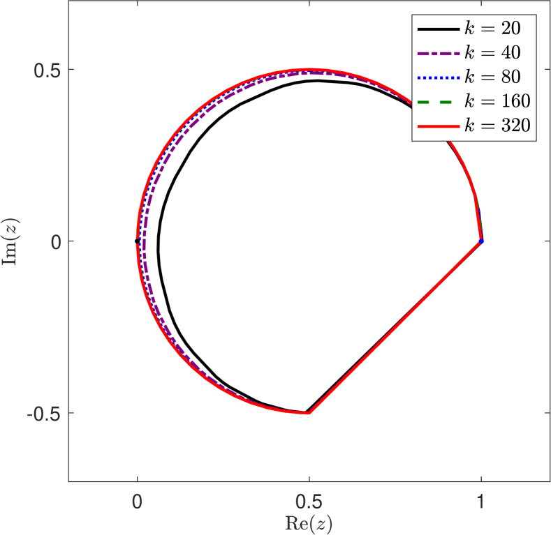
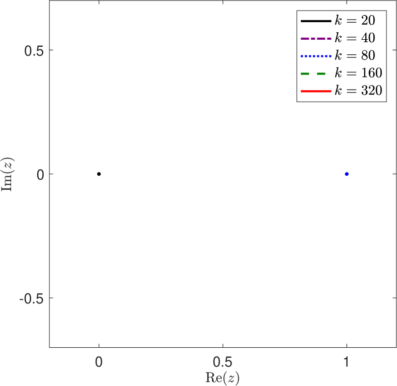
Figure 1: Field of values of $\mathbf{A}\mathbf{A}_{\varepsilon}^{-1}$ (left) and $\mathbf{A}\mathbf{B}_{\varepsilon}$ (right) for a 1D Helmholtz problem and various values of $k$, with $\varepsilon=k^{2}$ and $N_{H}\sim k^{2}$.

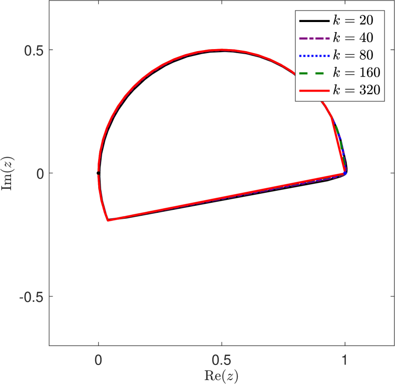
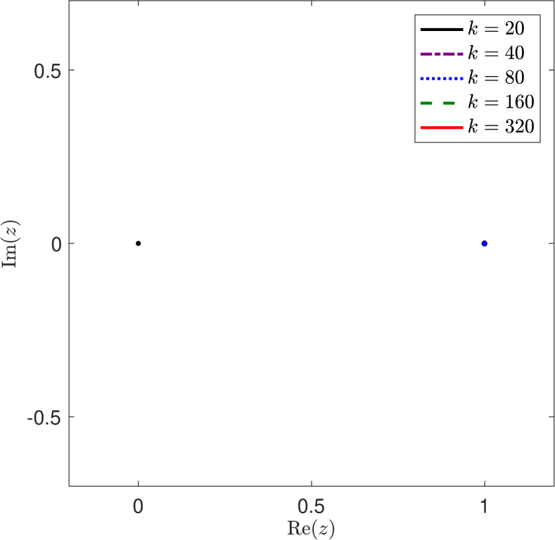
Figure 2: Field of values of $\mathbf{A}\mathbf{A}_{\varepsilon}^{-1}$ (left) and $\mathbf{A}\mathbf{B}_{\varepsilon}$ (right) for a 1D Helmholtz problem and various values of $k$, with $\varepsilon=5k^{2}$ and $N_{H}\sim k^{2}$.

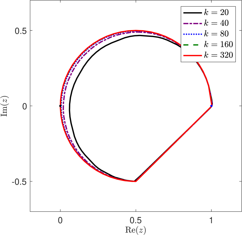
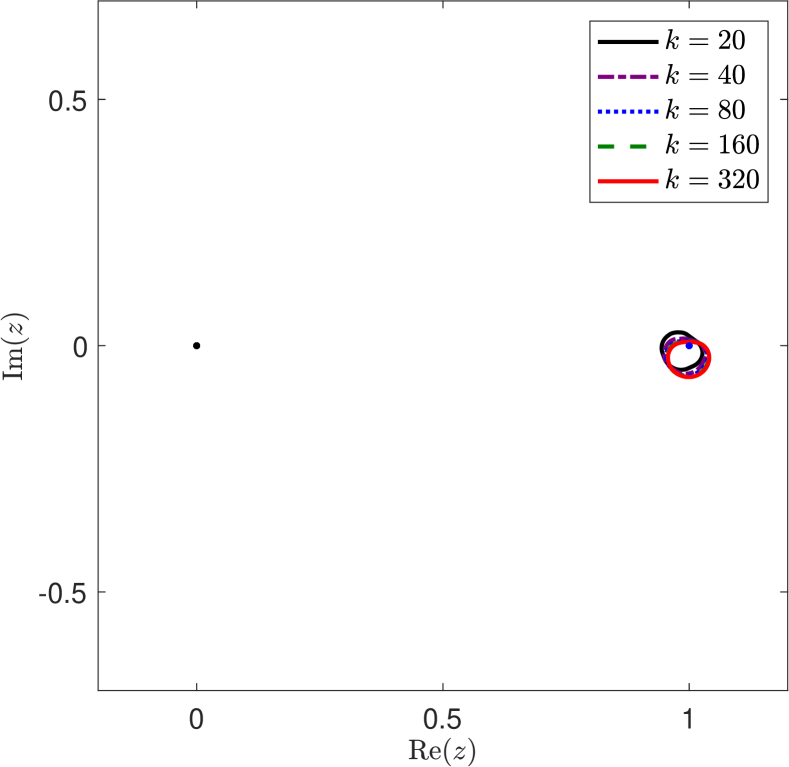
Figure 3: Field of values of $\mathbf{A}\mathbf{A}_{\varepsilon}^{-1}$ (left) and $\mathbf{A}\mathbf{B}_{\varepsilon}$ (right) for a 1D Helmholtz problem and various values of $k$, with $\varepsilon=k^{2}$ and $N_{H}\sim k^{3/2}$.

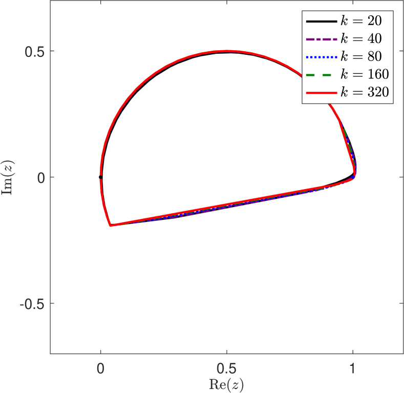
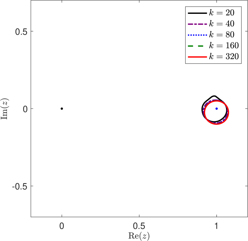
Figure 4: Field of values of $\mathbf{A}\mathbf{A}_{\varepsilon}^{-1}$ (left) and $\mathbf{A}\mathbf{B}_{\varepsilon}$ (right) for a 1D Helmholtz problem and various values of $k$, with $\varepsilon=5k^{2}$ and $N_{H}\sim k^{3/2}$.

Experiment 2

For our next experiment, we use GMRES to solve the interior impedance problem (1) on the unit square $(0,1)^{2}$, discretized with a uniform triangular grid. The right hand side is the constant vector of ones, and the initial guess the zero vector. We compare the complex shifted Laplace (CSL) preconditioner and the two-level preconditioner (TL) for various values of the shift $\varepsilon$ and distinct coarsening levels. The CSL preconditioner is inverted with one multigrid F(1,1) cycle with $\omega$-Jacobi smoothing on all levels, where $\omega=0.6$. The grid is chosen as follows: starting with a coarse grid with $3$ points in each direction, we refine the grid uniformly until we obtain a number of points (in one dimension) larger than $\lceil\alpha k^{3/2}\rceil$ where $\alpha=0.6$. The two-level preconditioner is tested using three different coarse grids. If $h$ is the fine meshsize in one dimension, the coarse meshsizes for the three different methods TL-1, TL-2 and TL-3 are $H=2h,4h,8h$ respectively. Since the coarse grid matrices are still large, we use an incomplete LU factorization with drop tolerance of $10^{-6}$ to simulate the exact solve of the coarse grid systems. The results are shown in table 1. Although the meshsize scales with $k^{-3/2}$ (not with $k^{-2}$, as required by the theory), the number of iterations remains constant when the coarse meshes of meshsize $2h$ and $4h$ are used. For the coarse meshsize $8h$ the number of iterations increases linearly, although at a much slower rate than the number of iterations of GMRES preconditioned by the standalone shifted Laplacian. This experiment shows that the theoretical results are not sharp and that wave-number independent convergence can be obtained also with pollution-free meshes where the mesh size scales with $k^{-3/2}$. Note that increasing the shift $\varepsilon$ leads to an increase in the number of iterations with the standalone CSL preconditioner, and for the wavenumbers $k=80$ and $k=100$ with the shift $\varepsilon=5k^{2}$ the GMRES method fails to reach the stopping criterion after 200 iterations. In contrast, the number of iterations remains bounded for the two-level preconditioner even for larger $\varepsilon$.

	$\varepsilon=k^{2}$				$\varepsilon=2k^{2}$				$\varepsilon=5k^{2}$
$k$	CSL	TL-1	TL-2	TL-3	CSL	TL-1	TL-2	TL-3	CSL	TL-1	TL-2	TL-3
$10$	14	7	8	10	19	7	9	12	29	7	11	17
$20$	26	7	10	16	38	7	11	20	65	7	13	29
$40$	45	6	9	17	79	6	9	19	146	6	9	22
$80$	78	7	12	36	149	7	12	42	-	7	12	46
$100$	99	6	9	21	184	6	9	22	-	6	9	23

Table 1: Experiment 2. Number of GMRES iterations for the Helmholtz linear system preconditioned by the CSL and the two-level method (TL) for various values of the shift $\varepsilon$ and different levels of coarsening.

Experiment 3

In our next experiment, we solve again the interior impedance problem (1) on the unit square $(0,1)^{2}$ with the same discretization, initial guess and right hand side as in our previous experiment, but this time we use a multilevel extension of the preconditioner, i.e., a multilevel Krylov method [13, 47]. This setting is not included in our theory but is more practically relevant since in realistic applications a two-grid preconditioner can be two expensive to apply. The multilevel preconditioner is implemented within a flexible GMRES (FGMRES) iteration [44], and every inexact coarse-grid solve (with a fixed small number of iterations) is performed by another FGMRES iteration, continuing (recursively) through all the grids until the coarsest grid is reached. For more details on the implementation of multilevel Krylov methods we refer the reader to [13, 36].

To set up a multilevel Krylov method requires fixing a number of iterations for the intermediate levels. We denote by MK$(l$,$m$,$n$) a method with $l,m,n$ iterations in the second, third and fourth level grid respectively, and one iteration in the remaining coarser grid levels. In this experiment we compare the CSL with the multilevel Krylov methods MK(8,4,2) and MK(6,4,2). The results are shown in Table 2. Similarly as in the two-level case, the multilevel preconditioner outperforms the CSL and requires a constant number of iterations to reach the desired tolerance, even though the intermediate coarse solves are done only inexactly with a small number of iterations. Note also that decreasing the number of iterations in the second level only increases the number of outer iterations by one or two, and the computation times of the two methods MK(8,4,2) and MK(6,4,2) are very similar.

	$\varepsilon=k^{2}$						$\varepsilon=2k^{2}$
	CSL		MK(8,4,2)		MK(6,4,2)		CSL		MK(8,4,2)		MK(6,4,2)
$k$	Iter	Time	Iter	Time	Iter	Time	Iter	Time	Iter	Time	Iter	Time
20	26	0.42	7	0.77	7	0.54	38	0.54	7	0.70	7	0.48
40	45	3.18	6	3.54	6	2.39	79	6.79	6	2.83	6	2.14
80	78	31.78	7	8.85	7	6.75	149	93.73	7	9.19	7	7.09
120	130	377.22	7	32.812	8	30.14	-	-	7	33.28	8	30.02
160	142	8121.02	6	124.87	8	129.24	-	-	7	150.37	8	127.34

Table 2: Experiment 3. Number of GMRES iterations and computation time (in seconds) for the Helmholtz linear system preconditioned by the CSL and the multilevel Krylov method (MK).

Experiment 4

In our final experiment we solve the impedance problem on the square $\Omega=(0,1)^{2}$ with a space-dependent wavenumber. This problem is adapted from [15]. The space-dependent wavenumber is given by

$$k(x,y)=\begin{cases}(4/3)k_{\text{ref}}&\text{if }0\leq y<0.2x+0.2\\ k_{\text{ref}}&\text{if }0.2x+0.2\leq y<-0.2x+0.8\\ 2k_{\text{ref}}&\text{if }-0.2x+0.8\leq y<1\end{cases}$$

where $k_{\text{ref}}>0$ is a reference wavenumber. This function is depicted in Figure 5. As the reference wavenumber $k_{ref}$ is varied, we choose the number of points for a uniform triangular mesh similarly as in the previous problems, with the number of points in one direction proportional to $\lceil\alpha k_{ref}^{3/2}\rceil$ with $\alpha=1.1$. The larger value of $\alpha$ is chosen to take into account the fact that the maximum wavenumber over the domain is $2k_{ref}$. Similarly to the previous experiments, the CSL preconditioner is compared here with the multilevel Krylov methods MK(8,4,2) and MK(6,4,2). The results are shown in Table 3. Similarly to the previous experiments, the number of iterations of the CSL preconditioner grows linearly with the wavenumber, and the number of iterations with either of the multilevel Krylov methods remains constant and the computation times are greatly reduced.

Figure 5: Space-dependent wavenumber in model problem 4.

	$\varepsilon=k^{2}$						$\varepsilon=2k^{2}$
	CSL		MK(8,4,2)		MK(6,4,2)		CSL		MK(8,4,2)		MK(6,4,2)
$k_{ref}$	Iter	Time	Iter	Time	Iter	Time	Iter	Time	Iter	Time	Iter	Time
20	33	1.23	6	2.02	6	0.96	52	1.44	6	1.17	6	0.87
40	60	24.16	6	8.01	6	6.22	105	59.96	6	7.68	6	5.97
60	81	132.98	5	23.42	6	22.63	153	424.3	5	25.53	6	21.7
80	106	239.8	6	31.24	7	34.10	194	649.99	6	28.01	7	25.27
100	126	7614.88	6	137.77	6	93.90	-	-	6	139.88	7	105.456

Table 3: Experiment 4. Number of GMRES iterations and computation time (in seconds) for the Helmholtz linear system with space-dependent wavenumber preconditioned by the CSL and the multilevel Krylov method (MK).

5 Conclusions

In this paper we have presented a two-level shifted Laplace preconditioner for Helmholtz problems discretised with finite elements. We used the convergence theory of GMRES based on the field of values to rigorously establish that GMRES will converge in a number of iterations independent of the wavenumber if a condition of the form $HK^{2}\leq C$ holds, for a constant $C$ independent of the wavenumber $k$ but possibly dependent on the size of the complex shift $\varepsilon$. We have also shown in numerical experiments that wavenumber independent convergence can also be obtained under the weaker condition $HK^{3/2}\leq C$, using a multilevel extension of the preconditioner (a multilevel Krylov method with inexact coarse grid solves), and for a test problem with heterogeneous wavenumber.

References

- [1] I. M. Babuška and S. A. Sauter, Is the Pollution Effect of the FEM Avoidable for the Helmholtz Equation Considering High Wave Numbers?, SIAM Rev., 42 (2000), pp. 451–484.
- [2] M. Benzi and M. A. Olshanskii, Field-of-Values Convergence Analysis of Augmented Lagrangian Preconditioners for the Linearized Navier–Stokes Problem, SIAM J. Numer. Anal., 49 (2011), pp. 770–788.
- [3] D. Braess, Finite Elements, Theory, Fast Solvers, and Applications in Solid Mechanics, Cambridge University Press, Apr. 2007.
- [4] A. Brandt and I. Livshits, Wave-ray multigrid method for standing wave equations, ETNA, 6 (1997), pp. 162–181 (electronic).
- [5] X. C. Cai and O. B. Widlund, Domain Decomposition Algorithms for Indefinite Elliptic Problems., SISC, 13 (1992), pp. 243–258.
- [6] L. Chen, FEM: an innovative finite element methods package in MATLAB, tech. report, University of California at Irvine, 2009.
- [7] P.-H. Cocquet and M. J. Gander, How Large a Shift is Needed in the Shifted Helmholtz Preconditioner for its Effective Inversion by Multigrid?, SIAM J. Sci. Comput., 39 (2017), pp. A438–A478.
- [8] S. Cools and W. Vanroose, Local Fourier analysis of the complex shifted Laplacian preconditioner for Helmholtz problems, Numer. Linear Algebra Appl. (NLAA), 20 (2013), pp. 575–597.
- [9] H. H. Elman, Iterative Methods for Large, Sparse, Nonsymmetric Systems of Linear Equations, PhD thesis, Yale University, 1982.
- [10] B. Engquist and L. Ying, Sweeping preconditioner for the Helmholtz equation: Hierarchical matrix representation, Communications on Pure and Applied Mathematics, 64 (2011), pp. 697–735.
- [11] , Sweeping Preconditioner for the Helmholtz Equation: Moving Perfectly Matched Layers, 9 (2011), pp. 686–710.
- [12] Y. A. Erlangga, Advances in iterative methods and preconditioners for the Helmholtz equation, Arch Computat Methods Eng, 15 (2007), pp. 37–66.
- [13] Y. A. Erlangga and R. Nabben, Multilevel Projection-Based Nested Krylov Iteration for Boundary Value Problems, SIAM J. Sci. Comput., 30 (2008), pp. 1572–1595.
- [14] , On a multilevel Krylov method for the Helmholtz equation preconditioned by shifted Laplacian, ETNA, (2008).
- [15] Y. A. Erlangga, C. Vuik, and C. W. Oosterlee, On a class of preconditioners for solving the Helmholtz equation, Applied Numerical Mathematics, 50 (2004), pp. 409–425.
- [16] , A novel multigrid-based preconditioner for heterogeneous Helmholtz problems, SIAM J. Sci. Comput., 27 (2006), pp. 1471–1492.
- [17] A. Ern and J.-L. Guermond, Theory and Practice of Finite Elements, vol. 159 of Applied Mathematical Sciences, Springer Science & Business Media, New York, NY, Mar. 2013.
- [18] O. G. Ernst and M. J. Gander, Why it is difficult to solve Helmholtz problems with classical iterative methods, in Numerical Analysis of Multiscale Problems, I. G. Graham, T. Y. Hou, O. Lakkis, and R. Scheichl, eds., Springer Science & Business Media, Berlin, Heidelberg, Jan. 2012.
- [19] S. Esterhazy and J. M. Melenk, On stability of discretizations of the Helmholtz equation (extended version), arXiv, (2011), pp. arXiv:1105.2112–324.
- [20] L. C. Evans, Partial Differential Equations, American Mathematical Soc., 2010.
- [21] M. J. Gander, I. G. Graham, and E. A. Spence, Applying GMRES to the Helmholtz equation with shifted Laplacian preconditioning: what is the largest shift for which wavenumber-independent convergence is guaranteed?, Numer. Math., 131 (2015), pp. 567–614.
- [22] M. J. Gander and H. Zhang, A Class of Iterative Solvers for the Helmholtz Equation: Factorizations, Sweeping Preconditioners, Source Transfer, Single Layer Potentials, Polarized Traces, and Optimized Schwarz Methods, SIAM Rev., 61 (2019), pp. 3–76.
- [23] L. García Ramos, R. Kehl, and R. Nabben, Projections, Deflation, and Multigrid for Nonsymmetric Matrices, SIAM J. Matrix Anal. & Appl., 41 (2020), pp. 83–105.
- [24] L. García Ramos and R. Nabben, On the Spectrum of Deflated Matrices with Applications to the Deflated Shifted Laplace Preconditioner for the Helmholtz Equation, SIAM J. Matrix Anal. & Appl., 39 (2018), pp. 262–286.
- [25] I. G. Graham, E. A. Spence, and E. Vainikko, Domain decomposition preconditioning for high-frequency Helmholtz problems with absorption, Math. Comp., 86 (2017), pp. 2089–2127.
- [26] I. G. Graham, E. A. Spence, and J. Zou, Domain Decomposition with local impedance conditions for the Helmholtz equation, arXiv, (2018).
- [27] A. Greenbaum, V. Pták, and Z. Strakoš, Any Nonincreasing Convergence Curve is Possible for GMRES, SIAM. J. Matrix Anal. & Appl., 17 (1996), pp. 465–469.
- [28] W. Hackbusch, Elliptic Differential Equations, vol. 18 of Springer Series in Computational Mathematics, Springer Berlin Heidelberg, Berlin, Heidelberg, 1992.
- [29] A. Hannukainen, Field of values analysis of preconditioners for the Helmholtz equation in lossy media, arXiv, (2011).
- [30] , Field of values analysis of a two-level preconditioner for the Helmholtz equation, SIAM J. Numer. Anal., 51 (2013), pp. 1567–1584.
- [31] U. Hetmaniuk, Stability estimates for a class of Helmholtz problems, Commun. Math. Sci., 5 (2007), pp. 665–678.
- [32] R. A. Horn and C. Johnson, Topics in Matrix Analysis, Cambridge University Press, June 1994.
- [33] F. Ihlenburg, Finite Element Analysis of Acoustic Scattering, vol. 132 of Applied Mathematical Sciences, Springer Science & Business Media, New York, 1998.
- [34] F. Ihlenburg and I. M. Babuška, Finite element solution of the Helmholtz equation with high wave number Part I: The h-version of the FEM, Computers & Mathematics with Applications, 30 (1995), pp. 9–37.
- [35] C. Johnson, Numerical Determination of the Field of Values of a General Complex Matrix, SIAM J. Numer. Anal., 15 (1978), pp. 595–602.
- [36] R. Kehl, R. Nabben, and D. B. Szyld, Adaptive Multilevel Krylov Methods, ETNA, 51 (2019), pp. 512–528.
- [37] D. Lahaye, J. M. Tang, and C. Vuik, Modern Solvers for Helmholtz Problems, Birkhäuser, Mar. 2017.
- [38] J. Liesen and Z. Strakoš, Krylov Subspace Methods, Principles and Analysis, Oxford University Press, Oct. 2012.
- [39] J. Liesen and P. Tichý, The field of values bounds on ideal GMRES, arXiv, (2018).
- [40] I. Livshits and A. Brandt, Accuracy properties of the wave-ray multigrid algorithm for Helmholtz equations, SIAM J. Sci. Comput., 28 (2006), pp. 1228–1251.
- [41] D. Loghin and A. J. Wathen, Analysis of Preconditioners for Saddle-Point Problems, SIAM J. Sci. Comput., 25 (2004), pp. 2029–2049.
- [42] J. Málek and Z. Strakoš, Preconditioning and the Conjugate Gradient Method in the Context of Solving PDEs, SIAM, Philadelphia, PA, Dec. 2014.
- [43] J. M. Melenk, On Generalized Finite Element Methods, PhD thesis, University of Maryland, 1995.
- [44] Y. Saad, A flexible inner-outer preconditioned GMRES algorithm, SIAM J. Sci. Comput., 14 (1993), pp. 461–469.
- [45] S. A. Sauter, A refined finite element convergence theory for highly indefinite Helmholtz problems, Computing, (2006).
- [46] A. H. Schatz, An observation concerning Ritz-Galerkin methods with indefinite bilinear forms, Math. Comp., 28 (1974), pp. 959–962.
- [47] A. H. Sheikh, D. Lahaye, L. García Ramos, R. Nabben, and C. Vuik, Accelerating the shifted Laplace preconditioner for the Helmholtz equation by multilevel deflation, Journal of Computational Physics, 322 (2016), pp. 473–490.
- [48] A. H. Sheikh, D. Lahaye, and C. Vuik, On the convergence of shifted Laplace preconditioner combined with multilevel deflation, Numer. Linear Algebra Appl. (NLAA), 20 (2013), pp. 645–662.
- [49] E. A. Spence, Overview of Variational Formulations for Linear Elliptic PDEs, in Unified Transform for Boundary Value Problems, Society for Industrial and Applied Mathematics, Philadelphia, PA, Jan. 2015, pp. 93–159.
- [50] G. Starke, Field-of-values analysis of preconditioned iterative methods for nonsymmetric elliptic problems, Numer. Math., 78 (1997), pp. 103–117.
- [51] U. Trottenberg, C. W. Oosterlee, and A. Schüller, Multigrid, Academic Press, 2001.
- [52] M. B. van Gijzen, Y. A. Erlangga, and C. Vuik, Spectral analysis of the discrete Helmholtz operator preconditioned with a shifted Laplacian, SIAM J. Sci. Comput., 29 (2007), pp. 1942–1958.
- [53] L. A. Zepeda-Núñez and L. Demanet, The method of polarized traces for the 2D Helmholtz equation, (2015), pp. 1–54.