Sound Algorithms in Imperfect Information Games

Abstract

Search has played a fundamental role in computer game research since the very beginning. And while online search has been commonly used in perfect information games such as Chess and Go, online search methods for imperfect information games have only been introduced relatively recently. This paper addresses the question of what is a sound online algorithm in an imperfect information setting of two-player zero-sum games. We argue that the fixed-strategy definitions of exploitability and $\epsilon$-Nash equilibria are ill-suited to measure an online algorithm’s worst-case performance. We thus formalize $\epsilon$-soundness, a concept that connects the worst-case performance of an online algorithm to the performance of an $\epsilon$-Nash equilibrium. As $\epsilon$-soundness can be difficult to compute in general, we introduce a consistency framework — a hierarchy that connects an online algorithm’s behavior to a Nash equilibrium. These multiple levels of consistency describe in what sense an online algorithm plays “just like a fixed Nash equilibrium”. These notions further illustrate the difference between perfect and imperfect information settings, as the same consistency guarantees have different worst-case online performance in perfect and imperfect information games. The definitions of soundness and the consistency hierarchy finally provide appropriate tools to analyze online algorithms in repeated imperfect information games. We thus inspect some of the previous online algorithms in a new light, bringing new insights into their worst-case performance guarantees.

1 Introduction

From the very dawn of computer game research, search was a fundamental component of many algorithms. Turing’s chess algorithm from $1950$ was able to think two moves ahead (Copeland 2004), and Shannon’s work on chess from $1950$ includes an extensive section on how an evaluation function can be used within search (Shannon 1950). Samuel’s checkers algorithm from $1959$ already combines search and learning of a value function, approximated through a self-play method and bootstrapping (Samuel 1959). The combination of search and learning has been a crucial component in the remarkable milestones where computers outperformed their human counterparts in challenging games: DeepBlue in Chess (Campbell, Hoane Jr, and Hsu 2002), AlphaGo in Go (Silver et al. 2017), DeepStack and Libratus in Poker (Moravcik et al. 2017; Brown and Sandholm 2018).

Online methods for approximating Nash equilibria in sequential imperfect information games appeared only in the last few years (Lisý, Lanctot, and Bowling 2015; Brown and Sandholm 2017; Moravcik et al. 2017; Brown and Sandholm 2018, 2019; Brown et al. 2020). We thus investigate what it takes for an online algorithm to be sound in imperfect information settings. While it has been known that search with imperfect information is more challenging than with perfect information (Frank and Basin 1998; Lisý, Lanctot, and Bowling 2015), the problem is more complex than previously thought. Online algorithms “live” in a fundamentally different setting, and they need to be evaluated appropriately.

Previously, a common approach to evaluate online algorithms was to compute a corresponding offline strategy by “querying” the online algorithm at each state (“tabularization” of the strategy) (Lisý, Lanctot, and Bowling 2015; Šustr, Kovařík, and Lisý 2019). One would then report the exploitability of the resulting offline strategy. We show that this is not generally possible and that naive tabularization can also lead to incorrect conclusions about the online algorithm’s worst-case performance. As a consequence we show that some algorithms previously considered to be sound are not.

We first give a simple example of how an online algorithm can lose to an adversary in a repeated game setting. Previously, such an algorithm would be considered optimal based on a naive tabularization. We build on top of this example to introduce a framework for properly evaluating an online algorithm’s performance. Within this framework, we introduce the definition of a sound and $\epsilon$-sound algorithm. Like the exploitability of a strategy in the offline setting, the soundness of an algorithm is a measure of its performance against a worst-case adversary. Importantly, this notion collapses to the previous notion of exploitability when the algorithm follows a fixed strategy profile.

We then introduce a consistency framework, a hierarchy that formally states in what sense an online algorithm plays “consistently” with an $\epsilon$-equilibrium. The hierarchy allows stating multiple bounds on the algorithm’s soundness, based on the $\epsilon$-equilibrium and consistency type. The stronger the consistency is in our hierarchy, the stronger are the bounds. This further illustrates the discrepancy of search in perfect and imperfect information settings, as these bounds sometimes differ for perfect and imperfect information games.

The definitions of soundness and the consistency hierarchy finally provide appropriate tools to analyze online algorithms in imperfect information games. We thus inspect some of the previous online algorithms in a new light, bringing new insights into their worst-case performance guarantees. Namely, we focus on the Online Outcome Sampling (OOS) (Lisý, Lanctot, and Bowling 2015) algorithm. Consider the following statement from the OOS publication: “We show that OOS is consistent, i.e., it is guaranteed to converge to an equilibrium strategy as search time increases. To the best of our knowledge, this is not the case for any existing online game playing algorithm…’ The problem is that OOS provides only the weakest of the introduced consistencies — local consistency. As the local consistency gives no guarantee for imperfect information games (in contrast to perfect information games), OOS (and potentially other locally consistent algorithms) can be highly exploited by an adversary. The experimental section then confirms this issue for OOS in two small imperfect information games.

2 Background

We present our results using the recent formalism of factored-observations stochastic games (Kovařík et al. 2019). The entirety of the paper trivially applies to the extensive form formalism (Osborne and Rubinstein 1994) as well (as we are only relying on the notion of states and rewards). We believe this choice of formalism makes it easier to incorporate our definitions in the future online algorithms, as sound search in imperfect information critically relies on the notion of common/public information (Burch, Johanson, and Bowling 2014; Seitz et al. 2019). Indeed, all the recently introduced online algorithms in imperfect information games rely on these notions (Moravcik et al. 2017; Brown and Sandholm 2018; Šustr, Kovařík, and Lisý 2019).

Definition 1.

A factored-observations stochastic game is a tuple

$$\mathcal{G}=\langle\mathcal{N},\mathcal{W},w^{o},\mathcal{A},\mathcal{T},\mathcal{R},\mathcal{O}\rangle,$$

where:

• $\mathcal{N}=\{1,\,2\}$ is a player set. We use symbol $n$ for a player and ${\textnormal{-}n}$ for its opponent.

• $\mathcal{W}$ is a set of world states and $w^{0}\in\mathcal{W}$ is a designated initial world state.

• $\mathcal{A}=\mathcal{A}_{1}\times\mathcal{A}_{2}$ is a space of joint actions. The subsets $\mathcal{A}_{n}(w)\subset\mathcal{A}_{n}$ and $\mathcal{A}(w)=\mathcal{A}_{1}(w)\times\mathcal{A}_{2}(w)\subset\mathcal{A}$ specify the (joint) actions legal at $w\in\mathcal{W}$. For $a\in\mathcal{A}$, we write $a=(a_{1},a_{2})$. $\mathcal{A}_{n}(w)$ for $n\in\mathcal{N}$ are either all non-empty or all empty. A world state with no legal actions is terminal.

• After taking a (legal) joint action $a$ at $w$, the transition function $\mathcal{T}$ determines the next world state $w^{\prime}$, drawn from the probability distribution $\mathcal{T}(w,a)\in\Delta(\mathcal{W})$.

• $\mathcal{R}=(\mathcal{R}_{1},\mathcal{R}_{2})$, and $\mathcal{R}_{n}(w,a)$ is the reward player $n$ receives when a joint action $a$ is taken at $w$.

• $\mathcal{O}=(\mathcal{O}_{\textnormal{priv(1)}},\mathcal{O}_{\textnormal{priv(2)}},\mathcal{O}_{\textnormal{pub}})$ is the observation function, where $\mathcal{O}_{(\cdot)}:\mathcal{W}\times\mathcal{A}\times\mathcal{W}\to\mathbb{O}_{(\cdot)}$ specifies the private observation that player $n$ receives, resp. the public observation that every player receives, upon transitioning from world state $w$ to $w^{\prime}$ via some joint action $a$.

A legal world history (or trajectory) is a finite sequence $h=(w^{0},a^{0},w^{1},a^{1},\,\dots\,,w^{t})$, where $w^{k}\in\mathcal{W}$, $a^{k}\in\mathcal{A}(w^{k})$, and $w^{k+1}\in\mathcal{W}$ is in the support of $\mathcal{T}(w^{k},a^{k})$. We denote the set of all legal histories by $\mathcal{H}$, and the set of all sub-sequences of $h$ that are legal histories as $\mathcal{H}(h)\subseteq\mathcal{H}$.

Since the last world state in each $h\in\mathcal{H}$ is uniquely defined, the notation for $\mathcal{W}$ can be overloaded to work with $\mathcal{H}$ (e.g., $\mathcal{A}(h):=\mathcal{A}(\textnormal{the last $w$ in $h$})$, $h$ being terminal, …). We use $\mathcal{Z}$ to denote the set of all terminal histories, i.e. histories where the last world state is terminal.

The cumulative reward of $n$ at $h$ is $\sum_{k=0}^{t-1}r^{k}_{n}:=\sum_{k=0}^{t-1}\mathcal{R}_{n}(w^{k},a^{k})$. When $h$ is a terminal history, cumulative rewards can also be called utilities, and denoted as $u_{n}(z)$. We assume games are zero-sum, so $u_{n}(z)=-u_{\textnormal{-}n}(z)\;\forall z\in\mathcal{Z}$. The maximum difference of utilities is $\Delta=\left|\max_{z\in\mathcal{Z}}u_{1}(z)-\min_{z\in\mathcal{Z}}u_{1}(z)\right|$

Player $n$’s information state or private history at $h=(w^{0},a^{0},w^{1},a^{1},\,\dots\,,w^{t})$ is the action-observation sequence $s_{n}(h):=(O^{0}_{n},a^{0}_{n},O^{1}_{n},a^{1}_{n},\,\dots\,,O^{t}_{n})$, where $O^{k}_{n}=\mathcal{O}_{n}(w^{k-1},a^{k-1},w^{k})$ and $O^{0}_{n}$ is some initial observation. The space $\mathcal{S}_{n}$ of all such sequences can be viewed as the private tree of $n$.

A strategy profile is a pair $\sigma=(\sigma_{1},\sigma_{2})$, where each (behavioral) strategy $\sigma_{n}:s_{n}\in\mathcal{S}_{n}\mapsto\sigma_{n}(s_{n})\in\Delta(\mathcal{A}_{n}(s_{n}))$ specifies the probability distribution from which player $n$ draws their next action (conditional on having information $s_{n}$). We denote the set of all strategies of player $n$ as $\Sigma_{n}$ and the set of all strategy profiles as $\Sigma$.

The reach probability of a history $h\in\mathcal{H}$ under $\sigma$ is defined as $\pi^{\sigma}(h)=\pi^{\sigma}_{1}(h)\,\pi^{\sigma}_{2}(h)\,\pi^{\sigma}_{c}(h),$ where each $\pi^{\sigma}_{n}(h)$ is a product of probabilities of the actions taken by player $n$ between the root and $h$, and $\pi^{\sigma}_{c}(h)$ is the product of stochastic transitions. The expected utility for player $n$ of a strategy profile $\sigma$ is $u_{n}(\sigma)=\sum_{z\in\mathcal{Z}}\pi^{\sigma}(z)u_{n}(z)$.

We define a best response of player $n$ to the other player’s strategies $\sigma_{{\textnormal{-}n}}$ as a strategy ${\mathpzc{br}}(\sigma_{{\textnormal{-}n}})\in\operatorname*{arg\,max}_{\sigma_{n}^{\prime}\in\Sigma_{n}}u_{n}(\sigma_{n}^{\prime},\sigma_{{\textnormal{-}n}})$ and best response value ${\mathpzc{brv}}(\sigma_{{\textnormal{-}n}})=\max_{\sigma_{n}^{\prime}\in\Sigma_{n}}u_{n}(\sigma_{n}^{\prime},\,\sigma_{{\textnormal{-}n}})$. The profile $\sigma$ is an $\epsilon$-Nash equilibrium if $\left(\forall\,n\in\mathcal{N}\right)\ :\ u_{n}(\sigma)\geq\max_{\sigma_{n}^{\prime}\in\Sigma_{n}}u_{n}(\sigma_{n}^{\prime},\sigma_{\textnormal{-}n})-\epsilon$, and we denote the set of all $\epsilon$-equilibrium strategies of player $n$ as $\mathcal{NE}^{\epsilon}_{n}$. The strategy exploitability is $\mathpzc{expl}\!_{n}(\sigma_{n}):=\big{[}u_{n}(\sigma^{*})-\min_{\sigma^{\prime}_{\textnormal{-}n}\in\Sigma_{\textnormal{-}n}}u_{n}(\sigma_{n},\sigma^{\prime}_{\textnormal{-}n})\big{]}$ where $\sigma^{*}$ is an equilibrium strategy. The game value $u^{*}=u_{1}(\sigma^{*})$ is the utility player 1 can achieve under a Nash equilibrium strategy profile.

3 Online Algorithm

The environment we are concerned with is that of a repeated game, consisting of a sequence of individual matches. As a match progresses, the algorithm produces a strategy for a visited information state on-line: that is, once it actually observes the state. This common framework of repeated games is particularly suitable for analysis of online algorithms, as the online algorithm can be conditioned on the past experience (e.g. by trying to adapt to the opponent or by re-using parts of the previous computation). We are then interested in the accumulated reward of the agent during the span of the repeated game. Of particular interest will be the expected reward against a worst-case adversary.

Coordinated Matching Pennies

We now introduce a small imperfect information game that will be used throughout the article – “Coordinated Matching Pennies” (CMP). It is a variation on the well-known Matching Pennies game (Osborne and Rubinstein 1994), where players choose either Heads or Tails and receive a utility of $\pm 1$ if their actions (mis)match. For CMP, we additionally introduce a publicly observable chance event just after the first player acts. See Figure 1 for details.

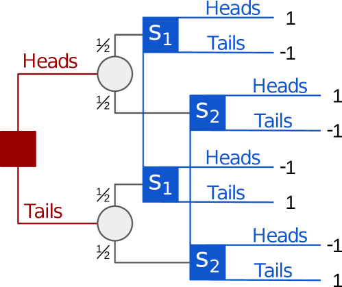
Figure 1: Coordinated Matching Pennies. After the first player acts, chance randomly chooses whether the second player will be playing in the information state $s_{1}$ or $s_{2}$. The first player receives utility of $1$ if players’ actions match and $-1$ if they mismatch.

Let $p$ and $q$ denote the probability of playing Heads in information states $s_{1}$ and $s_{2}$ respectively. An equilibrium strategy for the second player (Blue) is then any strategy where the average of $p$ and $q$ is $\frac{1}{2}$. He thus has to coordinate the actions between his two information states, while the first player has a unique uniform equilibrium strategy. Similar equilibrium coordination happens also in Kuhn Poker (Kuhn 1950).

Naive Tabularization

We now show that if one naively tries to convert an online algorithm into a fixed strategy, the resulting exploitability is not always representative of the worst-case performance of the online algorithm. Consider the following algorithm PlayCache for the repeated game of CMP. PlayCache keeps an internal state, a cache – a mapping of information state to probability distribution over the actions, and it gradually fills the cache during the game.

Concretely, PlayCache plays for the second player as follows:

• Initialize algorithm’s state $\bm{\theta}_{0}$ to an empty cache.

• Given an information state $s$ visited during a game, there are three possible cases: i) The cache is empty: play Heads and store $\{s,\text{Heads}\}$ into the cache. ii) The cache is non-empty and contains $s$: play the cached strategy for $s$. iii) The cache is non-empty and does not contain $s$: play Tails and store $\{s,\text{Tails}\}$.

Consider what happens if one tries to naively tabularize the PlayCache by querying the algorithm for all the information states. If we query the algorithm for states $s_{1},\ s_{2}$, we get the resulting offline strategy $s_{1}:\text{Heads},\ s_{2}:\text{Tails}$. Querying the algorithm for states in reverse order, i.e. $s_{2},\ s_{1}$ results in $s_{1}:\text{Tails},\ s_{2}:\text{Heads}$. And while both of these offline strategies have zero exploitability, one can still exploit the algorithm during the repeated game. This follows from the fact that the very first time the PlayCache gets to act, it always plays Heads. The first player can thus simply play Heads during the first match and is guaranteed to win the match. As we will show later, PlayCache falls within a class of algorithms that can be exploited, but where the average reward is guaranteed to converge to the game value as we repeatedly keep playing the game.

Where did this discrepancy between the exploitability of the tabularized strategy and the exploitability of the online algorithm come from? It is simply because the tabularized strategy does not properly describe the game dynamics of PlayCache. In fact, there is no fixed strategy that does so! We will now formalize an appropriate framework to describe the rewards and dynamics of online algorithms, which will allow us to define notions for the expected reward and the worst-case performance in the online setting.

Online Settings

The repeated game $p$ consists of a finite sequence of $k$ individual matches $m=(z_{1},\,z_{2},\,\ldots,\,z_{k})$, where each match $z_{i}\in\mathcal{Z}$ is a sequence of world states and actions $z_{i}=(w_{i}^{0},\,a_{i}^{0},\,w_{i}^{1},\,a_{i}^{1}\,\ldots,\,a_{i}^{l_{i}-1},w_{i}^{l_{i}})$, ending in a terminal world state $w_{i}^{l_{i}}$. For each visited world state in the match, there is a corresponding information state, i.e. a player’s private perspective of the game (for perfect information games, the notion of information state and world state collapse as the player gets to observe the world perfectly). An online algorithm $\Omega$ then simply maps an information state observed during a match to a strategy, while possibly using its internal algorithm state (Def. 2).

Given two players that use algorithms $\Omega_{1},\Omega_{2}$, we use $P^{k}_{\Omega_{1},\Omega_{2}}$ to denote the distribution over all the possible repeated games $m$ of length $k$ when these two players face each other. The average reward of $m$ is $\mathcal{R}_{n}(m)=1/k\sum_{i=1}^{k}u_{n}(z_{i})$ and we denote $\operatorname{\mathbb{E}}_{m\sim P^{k}_{\Omega_{1},\Omega_{2}}}[\mathcal{R}_{n}(m)]$ to be the expected average reward when the players play $k$ matches. From now on, if player $n$ is not specified, we assume without loss of generality it is player $1$. The proofs of the theorems can be found in the Appendix.

Definition 2.

Online algorithm $\Omega$ is a function $\mathcal{S}_{n}\times\Theta\mapsto\Delta(\mathcal{A}_{n}(s_{n}))\times\Theta$, that maps an information state $s_{n}\in\mathcal{S}_{n}$ to the strategy $\sigma_{n}(s_{n})\in\Delta(\mathcal{A}_{n}(s_{n}))$, while possibly making use of algorithm’s state $\bm{\theta}\in\Theta$ and updating it. We denote the algorithm’s initial state as $\bm{\theta}_{0}$. A special case of an online algorithm is a stateless algorithm, where the output of the function is independent of the algorithm’s state (thus independent of the previous matches). If the output depends on the algorithm’s state, we say the algorithm is stateful.

As the game progresses, the online algorithm produces strategies for the visited information states and updates its algorithm state. This allows it to potentially output different strategies for the same information state visited in different matches. We thus use $\Omega^{m}(s_{n})$ to denote the resulting strategy in the information state $s_{n}$ after the algorithm has already played the matches $m={z_{1},\,\ldots,\,z_{k}}$. Note that players can not visit the same information state twice in a single match.

Remark 3.

If we need to encode a stochastic algorithm, we can do it formally as taking the initial state to be a realization of a random variable. The initial state should be extended to encode how the algorithm should act (seemingly) randomly in any possible game-play situation beforehand.

Soundness of Online Algorithm

We are now ready to formalize the desirable properties of an online algorithm in our settings. Exploitability, resp. $\epsilon$-equilibrium considers the expected utility of a fixed strategy against a worst-case adversary in a single match. We thus define a similar concept for the settings of an online algorithm in a repeated game: $(k,\epsilon)$-soundness. Intuitively, an online algorithm is $(k,\epsilon)$-sound if and only if it is guaranteed the same reward as if it followed a fixed $\epsilon$-equilibrium after $k$ matches.

Definition 4.

For an $(k,\epsilon)$-sound online algorithm $\Omega$, the expected average reward against any opponent is at least as good as if it followed an $\epsilon$-Nash equilibrium fixed strategy $\sigma$ for any number of matches $k^{\prime}$:

$$\forall k^{\prime}\geq k\ \forall\Omega_{2}\,:\,\operatorname{\mathbb{E}}_{m\sim P^{k^{\prime}}_{\Omega,\Omega_{2}}}\left[\mathcal{R}(m)\right]\geq\operatorname{\mathbb{E}}_{m\sim P^{k^{\prime}}_{\sigma,\Omega_{2}}}\left[\mathcal{R}(m)\right].$$ (1)

If algorithm $\Omega$ is $(k,\epsilon)$-sound for $\forall k\geq 1$, we say the algorithm is $\epsilon$-sound.

Note that this definition guarantees that an online algorithm that simply follows a fixed $\epsilon$-equilibrium is $\epsilon$-sound. And while the online algorithm can certainly play as a fixed strategy, online algorithms are far from limited to doing so, e.g. PlayCache from Section 3. PlayCache is $1$-sound ($\epsilon=1$) as this algorithm is highly exploitable in the first match. Additionally, an online algorithm may be sound ($\epsilon=0$), but there might not be any offline equilibrium that produces the same distribution of matches.

Response Game

To compute the expected reward $\operatorname{\mathbb{E}}_{m\sim P^{k^{\prime}}_{\Omega,\Omega_{2}}}\left[\mathcal{R}(m)\right]$ as in Def. (4), we construct a repeated game (Osborne and Rubinstein 1994) in the FOSG formalism, where we replace the decisions of the online algorithm with stochastic (chance) transitions. As we allow the online algorithm to be stateful and thus produce strategies depending on the game trajectory, the response game must also reflect this possibility. The resulting game $\mathcal{G}^{k}_{\Omega}$ is thus exponential in size as it reflects all possible trajectories of $k$ matches. We call this single-player game a $k$-step response game.

The $k$-step response game allows us to compute the best response value of a worst-case adversary in $k$-match game-play. We will use overloaded notation ${\mathpzc{brv}}(\mathcal{G}^{k}_{\Omega})$ to denote this value.

Theorem 5.

If $\forall k^{\prime}\geq k\quad{\mathpzc{brv}}(\mathcal{G}^{k^{\prime}}_{\Omega})\leq k^{\prime}\epsilon$, then algorithm $\Omega$ is $(k,\epsilon)$-sound.

Proof.

If we used a fixed $\epsilon$-equilibrium strategy $\sigma$ in each match (repetition) of a response game $\mathcal{G}_{\sigma}^{k^{\prime}}$, then the ${\mathpzc{brv}}(\mathcal{G}_{\sigma}^{k^{\prime}})=k^{\prime}\epsilon$ because adversary can gain at most $\epsilon$ in each match. Since $\epsilon$-sound algorithm should play at least as well as some offline $\epsilon$-equilibrium, it must have ${\mathpzc{brv}}(\mathcal{G}_{\Omega}^{k})\leq{k}\epsilon\ \forall k\geq 1$. For a $(k,\epsilon)$-sound algorithm we add the condition of $\forall k^{\prime}\geq k$. ∎

Tabularized Strategy

When an online algorithm produces the same strategy for an information state regardless of the previous matches, there is no need for the $k$-response game. Fixed strategy notion sufficiently describes the behavior of the online algorithm and thus the exploitability of the fixed strategy matches the soundness. To compute this fixed strategy, one simply queries the online algorithm for all the information states in the game.

4 Relating $(k,\epsilon)$-Soundness and $\epsilon$-Nash

Unfortunately, our notion of $(k,\epsilon)$-soundness is often infeasible to reason about, as it requires checking that the algorithm does not make strategy errors for $\forall k^{\prime}\geq k$. In this section, we introduce the concept of consistency that allows one to formally state that the online algorithm plays “consistently” with an $\epsilon$-equilibrium. Our consistency notion allows us to directly bound the $(k,\epsilon)$-soundness of an online algorithm. We introduce three hierarchical levels of consistency, with varying restrictions and corresponding bounds. Notice that they differ mainly in the order of quantifiers.

Local Consistency

Local consistency simply guarantees that every time we query the online algorithm, there is an $\epsilon$-equilibrium that has the same local behavioral strategy $\sigma(s)$ for the queried state $s$.

Definition 6.

Algorithm $\Omega$ is locally consistent with $\epsilon$-equilibria if

$${\color[rgb]{0.0,0.0,0.0}\forall k\ \forall m=(z_{1},\,z_{2},\,\ldots,\,z_{k})}\ \ {\color[rgb]{0.0,0.0,0.0}\forall h\in\mathcal{H}(z_{k})}\ \ {\color[rgb]{0.0,0.0,0.0}\exists\sigma\in\mathcal{NE}^{\epsilon}_{n}}$$

$$\text{holds that}\ \ \Omega^{(z_{1},\,\ldots,\,z_{k-1})}(s(h))=\sigma(s(h)).$$

While this suggests that the algorithm plays like some equilibrium, it is not so, and the resulting strategy can be highly exploitable. This is because one cannot combine local behavioral strategies from different $\epsilon$-equilibria and hope to preserve their exploitability. In another perspective, as soon as one starts to condition the selection of the strategy on private information, it risks computing strategies that can be exploited in a repeated game. This is a motivation behind introducing $(k,\epsilon)$-soundness, as it allows us to analyze algorithms that use such conditioning.

Consider the CMP game with two strategies $\sigma^{1}=\{(s_{1},p=1),(s_{2},q=0)\}$ and $\sigma^{2}=\{(s_{1},p=0.5),(s_{2},q=0.5)\}$. While both strategies are equilibria, if one plays in the states $s_{1}$ and $s_{2}$ based on the first and second equilibrium respectively, it corresponds to an exploitable strategy $\{(s_{1},p=1),(s_{2},q=0.5)\}$.

Theorem 7.

An algorithm that is locally consistent with $\epsilon$-equilibria might not be $(k,\epsilon)$-sound.

Note that this can happen even in perfect information games. in Appendix A). Interestingly, local consistency is sufficient if the algorithm is consistent with a subgame perfect equilibrium.

Theorem 8.

In perfect information games, an algorithm that is locally consistent with a subgame perfect equilibrium is sound.

A particularly interesting example of an algorithm that is only locally consistent is Online Outcome Sampling (Lisý, Lanctot, and Bowling 2015) (OOS). See Section 6 for detailed discussion and experimental evaluation, where we show that this algorithm can produce highly exploitable strategies in imperfect information games.

Global Consistency

Local consistency guarantees consistency only for individual states. The problem we have then seen is that the combination of these local strategies might produce highly exploitable overall strategy. A natural extension is then to guarantee consistency with some equilibria for all the states in combination: a global consistency.

Definition 9.

Algorithm $\Omega$ is globally consistent with $\epsilon$-equilibria if

$${\color[rgb]{0.0,0.0,0.0}\forall k\ \forall m=(z_{1},\,z_{2},\,\ldots,\,z_{k})}\ \ {\color[rgb]{0.0,0.0,0.0}\exists\sigma\in\mathcal{NE}^{\epsilon}_{n}}\ \ {\color[rgb]{0.0,0.0,0.0}\forall h\in\mathcal{H}(z_{i})}$$

$$\text{holds that}\ \ \Omega^{(z_{1},\,\ldots,\,z_{i-1})}(s(h))=\sigma(s(h))\ \text{ for }\ \forall i\in\{1,\,\dots,\,k\}.$$

However:

Theorem 10.

An algorithm that is globally consistent with $\epsilon$-equilibria might not be $\epsilon$-sound.

Proof.

A counter-example: The PlayCache algorithm is globally consistent, but it is not sound ($\epsilon=0$), as we have seen that it is exploitable during the first match ($k=1$). ∎

But what if the algorithm keeps on playing the repeated game? While the global consistency with equilibria does not guarantee soundness, it guarantees that the expected average reward converges to the game value in the limit.

Theorem 11.

For an algorithm $\Omega$ that is globally consistent with $\epsilon$-equilibria,

$$\forall k\ \forall\Omega_{2}\,:\,\operatorname{\mathbb{E}}_{m\sim P^{k}_{\Omega,\Omega_{2}}}[\mathcal{R}(m)]\geq u^{*}-\epsilon-\frac{\bigl{|}\mathcal{S}_{1}\bigr{|}\Delta}{k}.$$ (2)

Corollary 12.

An algorithm $\Omega$ that is globally consistent with $\epsilon$-equilibria is $(k,\epsilon)$-sound as $k\rightarrow\infty$.

Strong Global Consistency

The problem with global consistency is that it guarantees the existence of consistent equilibrium for any game-play after the game-play is generated. Strong global consistency additionally guarantees that the game-play itself is generated consistently with an equilibrium; and as in global consistency, the partial strategies for this game-play also correspond to an $\epsilon$-equilibrium. In other words, the online algorithm simply exactly follows a predefined equilibrium.

Definition 13.

Online algorithm $\Omega$ is strongly globally consistent with $\epsilon$-equilibrium if

$${\color[rgb]{0.0,0.0,0.0}\exists\sigma\in\mathcal{NE}^{\epsilon}_{n}}\ \ {\color[rgb]{0.0,0.0,0.0}\forall k\ \forall m=(z_{1},\,z_{2},\,\ldots,\,z_{k})}\ \ {\color[rgb]{0.0,0.0,0.0}\forall h\in\mathcal{H}(z_{k})}$$

$$\text{holds that}\ \ \Omega^{(z_{1},\,\ldots,\,z_{k-1})}(s(h))=\sigma(s(h)).$$

Strong global consistency guarantees that the algorithm can be tabularized, and the exploitability of the tabularized strategy matches $\epsilon$-soundness of the online algorithm.

Theorem 14.

Online algorithm $\Omega$ that is strongly globally consistent with $\epsilon$-equilibrium is $\epsilon$-sound.

Canonical examples of strongly globally consistent online algorithms are DeepStack/Libratus. In general, an algorithm that uses a notion of safe (continual) resolving is strongly globally consistent as it essentially re-solves some $\epsilon$-equilibrium (albeit an unknown one) that it follows. Another, more recent example is ReBeL (Brown et al. 2020), as it essentially imitates CFR-D iterations in conjunction with a neural network.

Proving Strong Global Consistency

While we are not aware of an algorithm that is only globally consistent (besides the toy PlayCache), reasoning about global consistency can be beneficial for showing the strong global consistency. Doing so just based on its definition might not be straightforward. However, proving global consistency can be easier. If applicable, we can then use the following theorem to extend the proof to the strong global consistency.

Theorem 15.

If a globally consistent algorithm is stateless then it is also strongly globally consistent.

Proof.

The definition of a stateless algorithm implies that for an information state $s$ the algorithm always produces the same behavioral strategy $\sigma(s)$ as the algorithm is deterministic (all stochasticity is encoded within the algorithm state $\bm{\theta}$, see Remark 3).

This means that whatever $\epsilon$-equilibria the algorithm is globally consistent with is independent of the current game-play or match number. This allows us to swap the quantifiers from

$${\color[rgb]{0.0,0.0,0.0}\forall k\ \forall m=(z_{1},\,z_{2},\,\ldots,\,z_{k})}\ {\color[rgb]{0.0,0.0,0.0}\exists\sigma\in\mathcal{NE}^{\epsilon}_{n}}\ {\color[rgb]{0.0,0.0,0.0}\forall i\in\{1,\,\dots,\,k\}\ \forall h\in\mathcal{H}(z_{i})}\ :$$

$$\Omega^{(z_{1},\,\ldots,\,z_{i-1})}(s(h))=\sigma(s(h))$$

to

$${\color[rgb]{0.0,0.0,0.0}\exists\sigma\in\mathcal{NE}^{\epsilon}_{n}}\ {\color[rgb]{0.0,0.0,0.0}\forall k\ \forall m=(z_{1},\,z_{2},\,\ldots,\,z_{k})}\ {\color[rgb]{0.0,0.0,0.0}\forall i\in\{1,\,\dots,\,k\}\ \forall h\in\mathcal{H}(z_{i})}\ :$$

$$\Omega^{(z_{1},\,\ldots,\,z_{i-1})}(s(h))=\sigma(s(h)).$$

Using the same argument we can treat the different matches $z_{i}$ as an iteration over $k$, leading us to strong global consistency

$${\color[rgb]{0.0,0.0,0.0}\exists\sigma\in\mathcal{NE}^{\epsilon}_{n}}\ {\color[rgb]{0.0,0.0,0.0}\forall k\ \forall m=(z_{1},\,z_{2},\,\ldots,\,z_{k})}\ {\color[rgb]{0.0,0.0,0.0}\forall h\in\mathcal{H}(z_{k})}\ :$$

$$\Omega^{(z_{1},\,\ldots,\,z_{k-1})}(s(h))=\sigma(s(h)).$$

∎

5 Relating $(k,\epsilon)$-Soundness and Regret

Regret is an online learning concept that has triggered design of a family of powerful learning algorithms. Indeed, many algorithms that approximate Nash equilibria use regret minimization (Zinkevich et al. 2008). There is a well-known connection between regret and the Nash equilibrium solution concept. In a zero-sum game at time $k$, if both players’ overall regret $R_{k}$ is less than $k\epsilon$, the average strategy profile is a $2\epsilon$-equilibrium (Zinkevich et al. 2008). The use of $k$ in $(k,\epsilon)$-soundness allows us to relate it with regret, and show how it is different from the consistency hierarchy.

Corollary 16.

Any regret minimizer with a regret bound of $R_{k}$ is $(k,\frac{R_{k}}{2k})$-sound.

6 Experiments

A particularly interesting example of an algorithm that is only locally consistent is Online Outcome Sampling (OOS) (Lisý, Lanctot, and Bowling 2015). We use it to demonstrate the theoretical ideas in this paper with empirical experiments. We show that local consistency does in fact fail to result in $\epsilon$-soundness in the online setting. The problem we demonstrate is also not specific to OOS, but in general to any adaptation of an offline algorithm to the online setting where the algorithm attempts to improve its strategy during online play.

At high level, OOS runs the offline MCCFR algorithm in the full game (while also gradually building the tree), parameterized to increase the sampling probability of the current information state. The algorithm then plays based on the resulting strategy for that particular state. The problem is that these individual MCCFR runs can converge to different $\epsilon$-equilibria as the MCCFR is parameterized differently in each information state. In other words, the OOS algorithm exactly suffers from the fact that it is only locally consistent.

We use two games in our experiments: Coordinated Matching Pennies from Section 3 and Kuhn Poker (Kuhn 1950). We present the Coordinated Matching Pennies results here. See Appendix D for the complete experimental details and a similar experiment for Kuhn Poker.

Within a single match of Coordinated Matching Pennies, the second player will act either in $s_{1}$ or $s_{2}$. OOS will therefore bias MCCFR samples to whichever information state that actually occurs in the match. These two situations are distinct and result in two different strategies for the whole game (including the non-visited state), similarly to the example in Section 4. To emulate what OOS does, we parametrize MCCFR runs to bias samples into $s_{1}$ and $s_{2}$ respectively, and initialize the regrets in $s_{1},s_{2}$ so that the MCCFR is likely to produce diverse sets of strategies. As MCCFR is stochastic, we average the strategies over $3\cdot 10^{4}$ random seeds.

In Figure 2 we plot exploitability for the average strategies, and unbiased MCCFR for reference. The two biased variants of MCCFR actually converge at a similar rate to unbiased MCCFR, confirming that OOS is locally consistent: it quickly converges to an $\epsilon$-equilibria for $s_{1}$ and $s_{2}$ individually. However, the tabularized strategy — the strategy OOS follows online — is many orders of magnitude more exploitable even with hundreds of thousands of online iterations. The problem is that adapting its strategy online at $s_{1}$ and $s_{2}$ causes it to not be globally consistent with any $\epsilon$-equilibria.

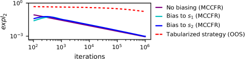
Figure 2: While individual MCCFR strategies have low exploitability of $\sim 10^{-3}$, the tabularized OOS strategy has high exploitability of $0.17$ even after $10^{6}$ iterations.

7 Related literature

There are several known pathologies that occur in imperfect information games that are not present in the perfect information case. The pathologies that happen in the offline setting also present a problem in the online setting. In (Frank and Basin 1998) the authors identified two problems: strategy-fusion and non-locality.

These two problems can easily arise for algorithms designed to solve only perfect-information games, such as minimax or reinforcement learning algorithms, and lead to computation of exploitable strategies. The proposed local consistency is similar in its spirit to non-locality, as composition of partial strategies (that correspond to parts of distinct equilibria) produced by an online algorithm may not be an overall equilibrium strategy. However local consistency identifies sub-optimal play also across repeated games.

In (Moravcik et al. 2017; Brown and Sandholm 2018), they use some form of continual re-solving, which is strongly globally consistent. This guarantees soundness of the algorithms. Continual resolving uses value functions defined over public belief spaces (Brown et al. 2020) to compute consistent strategies. Indeed, the minimal amount of information needed to properly define value functions are ranges (beliefs) over common knowledge public states (Seitz et al. 2019).

The notion of sufficient plan-time statistics studied in (Oliehoek13IJCAI) is very closely related to the public beliefs. The paper suggests the structure of the value function for games where the hidden information becomes public after a certain number of moves.

We are not aware of algorithms in the literature that are only globally consistent. This may lead to interesting future work: the algorithm may try to reduce its sub-optimal play of the first matches, while possibly not using all of the required player’s ranges.

Tabularization has been used in (Šustr, Kovařík, and Lisý 2019) to compute an offline strategy and its exploitability. In (Lisý, Lanctot, and Bowling 2015) they consider computing this tabularization (they refer to it as “brute-force” approach), but it is a very expensive procedure. Instead they use an “aggregate method”, which “stitches” strategy from a small number of matches and defines the strategy as uniform in non-visited information states. They do not state whether such approximation of tabularization is indeed correct.

8 Conclusion

We introduced the game of Coordinated Matching Pennies (CMP). This game illustrates the consistency issues that can arise for online algorithms in imperfect information games. We observed that exploitability is not an appropriate measure of an algorithm’s performance in online settings. This motivated us to introduce a formal framework for studying online algorithms and allowed us to define $\epsilon$-soundness. Just like $\epsilon$-exploitability, it measures the performance against the worst-case adversary. Soundness generalizes exploitability to repeated sequential games and it collapses to it when an online algorithm follows a fixed strategy. We then introduced a hierarchical consistency framework that formalizes in what sense an online algorithm can be consistent with a fixed strategy. Namely, we introduced three levels of consistency: i) local, ii) global and iii) strongly global. These connect an online algorithm’s behavior to that of a fixed strategy with increasingly tight bounds on the average expected utility against a worst-case adversary. We also stated various bounds on soundness based on the exploitability of a consistent fixed strategy. Interestingly, the implications are different in some cases for perfect and imperfect information games.

Within this framework, we saw that local consistency in imperfect information games does not guarantee correct evaluation of worst-case performance by computing exploitability. Based on this result, we argued that OOS, previously considered sound, can be exploited. This illustrates that these subtle problems with online algorithms can easily be missed and lead to wrong conclusions about their performance. Our experimental section included experiments in CMP and Kuhn Poker and showed a large discrepancy between OOS’s actual performance and the bound previously thought to hold.

Acknowledgments

Computational resources were supplied by the project ”e-Infrastruktura CZ” (e-INFRA LM2018140) provided within the program Projects of Large Research, Development and Innovations Infrastructures. This work was supported by Czech science foundation grant no. 18-27483Y. We’d like to thank the anonymous reviewers for their valuable feedback on a prior version of this paper.

Appendix A Consistency Examples

Example 17.

An online algorithm may be sound ($\epsilon=0$), but there might not be any offline equilibrium that produces the same distribution of matches.

Suppose we have a game where each player acts once, chooses from actions $\{A,B,C\}$ and receives zero utility (i.e. a normal-form game with 3x3 zero payoff matrix). All strategies are equilibria. If we play $k=3$ matches and the players play pure strategies $A$, $B$ and $C$ in each match, we get a distribution of matches $m=(z_{1},z_{2},z_{3})$ that cannot be achieved with fixed offline equilibrium. In this case, the distribution is $((w^{0},(A,A)),(w^{0},(B,B)),(w^{0},(C,C)))$ with probability one, and all other terminal histories with probability zero.

Example 18.

An algorithm that is locally consistent with equilibria can be exploited in a perfect information game.

Suppose we have a single player game as in figure on the right. Both blue $L,Y$ and red $R,X$ pure strategies are equilibria. However, if the top node is locally consistent with the blue strategy, and the bottom node with the red strategy, the resulting strategy the algorithm actually plays is $L,X$, which is sub-optimal.

Appendix B Tabularization

We can consider two ways how the online setting can be realized, with respect to how players’ state changes between $k$ matches in the repeated game: i) no-memory, where the players take turns in a match, and their memory is reset when each match is over (players are allowed to retain memory within the individual matches), or ii) with-memory, where the players are allowed to retain memory between the matches.

As exploitability of tabularized strategy is guaranteed to reflect $\epsilon$-soundness only for strongly globally consistent algorithms, we assume their use only. The with-memory case then collapses to the no-memory case: strongly globally consistent algorithm simply plays as some predefined (offline) equilibrium. The following text then simply defines how to compute the offline equilibrium by querying the algorithm in all states.

Definition 19 (Partial strategy).

For a terminal history

$$z=(w^{0}\!\!,\,a^{0},\,w^{1}\!\!,\,a^{1},\,\ldots,\,w^{l}\!\!,\,a^{l},\,w^{l+1})$$

player $n$ has a corresponding sequence of information states

$$s=(s^{0}\!\!,\,s^{1}\!\!,\,\ldots,\,s^{l},\,s^{l+1}).$$

We say a partial strategy $\sigma^{\Omega,\!\bm{\theta}_{0}}_{n}(z)$ for player $n$ who uses search $\Omega$ and starts with state $\bm{\theta}_{0}$, is an expected behavioral strategy defined only for the visited information states:

$$\sigma^{\Omega,\!\bm{\theta}_{0}}_{n}(z)=\{(s^{t},\,\mu_{t})\mid(\mu_{t},\bm{\theta}_{t+1})=\operatorname{\mathbb{E}}_{\bm{\theta}_{t}}\left[\Omega(s^{t},\bm{\theta}_{t})|s^{t}\right]\>\forall\,t\in\{0,\dots,l\}\}.$$

Note that when we compute the strategy $\mu_{t}$ from $\operatorname{\mathbb{E}}_{\bm{\theta}_{t}}\left[\Omega(s^{t},\bm{\theta}_{t})|s^{t}\right]$, we must compute it as a weighted average to respect the structure of the private tree. The weights are reach probabilities of the information state $s^{t}$: cumulative product of the player’s strategy over the sequence of information states $s^{0},\ldots s^{t-1}$, leading to target information state $s^{t}$. See (Zinkevich et al. 2008, Eq. 4) for more details.

Definition 20.

A composition of partial strategies for terminals $\mathcal{Z}$ is a tabularized strategy

$$\sigma^{\Omega,\!\bm{\theta}_{0}}_{n}(\mathcal{Z})=\bigcup_{z_{i}\in\mathcal{Z}}\sigma^{\Omega,\!\bm{\theta}_{0}}_{n}(z_{i}).$$

Appendix C Proofs of Theorems

See 8

Proof.

In perfect information games the notions of an information state and a history blend together, as there is a one-to-one correspondence between them. Expected utility of a history is the same for all subgame perfect equilibria. It corresponds to the best achievable value against worst-case adversary, given that the history occurred. This property implies that the worst-case expected utility of a history remains optimal, if the player plays only actions that are in the support of any subgame perfect equilibrium in the consequent states. A formal proof can be constructed by induction on the maximal distance from a terminal history.

Notice that this exactly happens if the player plays according to an algorithm locally consistent with subgame perfect equilibria. The expected worst-case utility for any history will be optimal, and the worst-case expected utility of a match will correspond to the worst-case expected utility of the history at the beginning of the game. Therefore the worst-case expected utility of each match is also optimal and the algorithm is sound. ∎

We will now prepare the ground to prove Thm. 11.

When an algorithm that is globally consistent with an $\epsilon$-equilibrium is queried in some information states in a match in the repeated game, it will always keep playing the same behavioral strategy in these situations in subsequent matches. We call this as “filling in” strategy. Once the algorithm fills the strategy in all player’s information states, we are guaranteed to get match reward of $u^{\epsilon}=u^{*}-\epsilon$ on average against a worst-case adversary.

Informally speaking, the bound in Thm. 11 can be easily seen to be true for a game like Coordinated Matching Pennies, or some generalization which will have a larger number of information states that need to be coordinated (think of “Coordinated Rock-Paper-Scissors”). At every match, we can incur a loss of at most $\Delta$ when reaching an unfilled history. This is a rather pessimistic lower bound on the value, but it lets us ignore the algorithm state: we are either playing at filled information states, or achieving the worst possible value. The problematic part is making sure the bound holds also when we (repeatedly) visit previously filled information states. For each of the possible future subgames, there are two cases. In both cases, the number of $\Delta$-sized losses in utility plus the number of unfilled information states does not increase, so we can use induction on the length of the game to prove the claim. Along branches where the opponent had an opportunity to exploit the algorithm by playing into an unfilled information state, the algorithm loses at most $\Delta$ utility compared to the equilibrium, but must fill in at least one information state to do so. Along branches where the agent played through filled information states, the algorithm is playing identically to the equilibrium strategy and thus achieves the same value.

To prove Thm. 11 we will need to establish a Lemma 21, a bound of difference of utilities a player can gain if he plays according to a partially filled $\epsilon$-equilibrium strategy compared to $u^{\epsilon}$ within an arbitrary match. The idea of the proof for Thm. 11 is then to bound this difference for any number of non-visited information states and any number of remaining matches within the response game using induction.

An online algorithm can fill in the strategy only into information states found on the trajectory to a terminal history, as it will be queried only in these situations. So after playing through a match $z=(w^{0}\!\!,\,a^{0},\,w^{1}\!\!,\,a^{1},\,\ldots,\,w^{l}\!\!,\,a^{l},\,w^{l+1})$, the algorithm’s response at $s_{n}(w^{i})$ will be fixed as $\sigma(s_{n}(w^{i}))$ for all visited worlds $w^{i}$ on the trajectory $z$.

To talk about possible filled strategies within a single match, we will partition $\mathcal{Z}$ into two non-empty sets of terminal histories $\mathcal{Z}_{\bullet}$ (pronounced “filled”) and $\mathcal{Z}_{\circ}$ (pronounced “empty” or “unfilled”). The partition has a special property of “being possible to realize in online setting”: all information states on the trajectory to terminals $\mathcal{Z}_{\bullet}$ are filled, and all terminals that can be reached just through these filled information states are also in $\mathcal{Z}_{\bullet}$ (we are not taking into consideration the opponent’s information states, i.e. we operate only on the online player’s private tree).

Lemma 21.

For a probability of reaching a filled terminal $P({\bullet})=\sum_{z_{\bullet}\in\mathcal{Z}_{\bullet}}\pi^{\sigma}(z_{\bullet})$, an expected received utility for filled terminals $u({\bullet})=\frac{\sum_{z_{\bullet}\in\mathcal{Z}_{\bullet}}\pi^{\sigma}(z_{\bullet})u_{1}(z_{\bullet})}{\sum_{z_{\bullet}\in\mathcal{Z}_{\bullet}}\pi^{\sigma}(z_{\bullet})}$ and an utility of playing outside of filled histories $u({\times})$, it holds that

$$P({\bullet})(u({\bullet})-u^{\epsilon})\geq-(1-P({\bullet}))(u({\times})-u^{\epsilon}+\Delta),$$ (3)

assuming $0<P({\bullet})<1$.

Proof.

For any strategy profile $\sigma=(\sigma_{1}^{\epsilon},\sigma_{2})$ with an $\epsilon$-equilibrium strategy $\sigma_{1}^{\epsilon}$ and arbitrary opponent strategy $\sigma_{2}$ it holds that

$$\sum_{z_{\bullet}\in\mathcal{Z}_{\bullet}}\pi^{\sigma}(z_{\bullet})u_{1}(z_{\bullet})+\sum_{z_{\circ}\in\mathcal{Z}_{\circ}}\pi^{\sigma}(z_{\circ})u_{1}(z_{\circ})\geq u^{\epsilon}.$$ (4)

The terms can be simplified and rewritten as factorization of product of probabilities and (weighted) utilities as

$$P({\bullet})u({\bullet})=\underbrace{\sum_{z_{\bullet}\in\mathcal{Z}_{\bullet}}\pi^{\sigma}(z_{\bullet})}_{P({\bullet})}\cdot\underbrace{\frac{\sum_{z_{\bullet}\in\mathcal{Z}_{\bullet}}\pi^{\sigma}(z_{\bullet})u_{1}(z_{\bullet})}{\sum\limits_{z_{\bullet}\in\mathcal{Z}_{\bullet}}\pi^{\sigma}(z_{\bullet})}}_{u({\bullet})},$$

and similarly for the “${\circ}$” partition. It also holds that $P({\bullet})+P({\circ})=1$, as the probability of reaching a terminal history within a match is equal to one.

We can restate (4) as

$$P({\bullet})(u({\bullet})-u^{\epsilon})+(1-P({\bullet})(u({\circ})-u^{\epsilon})\geq 0.$$ (5)

Suppose that for the partition “${\circ}$” we didn’t use an equilibrium strategy for player 1, but arbitrary strategy profile $\sigma^{\prime}$ satisfying $P^{\sigma}({\bullet})+P^{\sigma^{\prime}}({\circ})=1$. We will denote its utility

$$u({\times})=\frac{\sum_{z_{\circ}\in\mathcal{Z}_{\circ}}\pi^{\sigma^{\prime}}(z_{\circ})u_{1}(z_{\circ})}{\sum_{z_{\circ}\in\mathcal{Z}_{\circ}}\pi^{\sigma^{\prime}}(z_{\circ})}.$$ (6)

The value of any two strategies cannot differ by more than the maximum difference of utilities in the game:

$$u({\circ})\leq u({\times})+\Delta.$$ (7)

Putting (7) back to (5), we get the lemma that lower bounds the difference of filled partition and $u^{\epsilon}$ for an arbitrary match:

$$P({\bullet})(u({\bullet})-u^{\epsilon})\geq-(1-P({\bullet}))(u({\times})-u^{\epsilon}+\Delta).$$ (8)

∎

See 11

Proof.

Let us rewrite the theorem slightly:

$$\forall k\ \forall\Omega_{2}\,:\,k\operatorname{\mathbb{E}}_{m\sim P^{k}_{\Omega,\Omega_{2}}}[\mathcal{R}(m)]-ku^{\epsilon}\geq-\bigl{|}\mathcal{S}_{1}\bigr{|}\Delta.$$

Since $\mathcal{R}(m)$ is average reward, multiplying by $k$ we get cumulative utilities in the game-play $m=(z_{1},z_{2},\,\dots,\,z_{k})$:

$$\forall k\ \forall\Omega_{2}\,:\,\operatorname{\mathbb{E}}_{m\sim P^{k}_{\Omega,\Omega_{2}}}\left[\sum_{i=1}^{k}u_{1}(z_{i})\right]-ku^{\epsilon}\geq-\bigl{|}\mathcal{S}_{1}\bigr{|}\Delta.$$ (9)

So on the left side of the inequality we have a difference of cumulative (expected) utilities and of cumulative $u^{\epsilon}$. We use cumulative values because we are now in the setting of a $k$-repeated game.

Let $v$ be the number of non-visited information states of player 1 (resp. the number of unfilled information states) in a match, i.e. $0\leq v\leq|\mathcal{S}_{1}|$, and let $l$ be the number of next matches (including the current one), i.e. $1\leq l\leq k$. We will use $a_{v,l}$ to denote the difference between expected cumulative rewards and cumulative $u^{\epsilon}$ from the current match (inclusively) until the end of the game, if we are playing against worst-case adversary. The left side of (9) corresponds to a value equal or greater than $a_{|\mathcal{S}_{1}|,k}$, so we need to prove that $a_{|\mathcal{S}_{1}|,k}\geq-\bigl{|}\mathcal{S}_{1}\bigr{|}\Delta$. It is sufficient to consider only the worst-case adversary, as the bound on $a_{v,l}$ will hold for any other opponent as well.

We will prove the theorem by induction on $a_{v,l}$ using $v$ and $l$ simultaneously. Let us characterize the base case. If we have visited all information states ($v=0$), we filled $\epsilon$-equilibrium strategy everywhere. So at each visit of such a match we receive a reward of $u^{\epsilon}$, and the difference between expected cumulative rewards and cumulative $u^{\epsilon}$ is zero:

$$a_{0,l}=0\quad\forall l.$$ (10)

The induction hypothesis is

$$a_{x,y}\geq-x\Delta\quad\forall x\leq v\ \forall y<l.$$ (11)

There are two possibilities of what can happen in a match. We either “hit” the filled information states, receive some (expected) reward $u(v,l)$ and possibly continue into next match where we receive $a_{v,l-1}$ (if the current match is not the last one, i.e. $l>1$). Or we “miss” the filled information states, meaning we visit arbitrary number of new information states previously not visited. This will also change $v$ to be smaller for all subsequent matches.

We state this with an abuse of notation as

$$a_{v,l} =P(v,l)(u(v,l)-u^{\epsilon}+a_{v,l-1})$$ (12)

$$+P(v-1,l)(u(v-1,l)-u^{\epsilon}+a_{v-1,l-1})$$

$$+P(v-2,l)(u(v-2,l)-u^{\epsilon}+a_{v-2,l-1})$$

$$+\ \dots$$

$$+P(v-v,l)(u(v-v,l)-u^{\epsilon}+a_{v-v,l-1}),$$

where the terms $P(v-i,l)$ and $u(v-i,l)$ are defined similarly to how we defined them for $P({\bullet})$ and $u({\bullet})$. They correspond to the probability and utilities received when we visit $i$ new (previously unfilled) information states with $l$ remaining matches (including current one). It holds that $P(v,l)+P(v-1,l)+P(v-2,l)+\dots+P(v-v,l)=1$ as the probability of reaching a terminal history within a match is equal to one.

By using the induction hypothesis (11) on terms $a_{x,l-1}\ \forall x<v$ we get a lower bound $a_{x,l-1}\geq-x\Delta$ on all of $x$. By comparing these bounds we can deduce that $a_{v-1,l-1}$ lower bounds all of $a_{x,l-1}$ with

$$a_{v-1,l-1}\geq-(v-1)\Delta.$$ (13)

Using this bound in (12) we get

$$a_{v,l}\geq P(v,l)(u(v,l)-u^{\epsilon}+a_{v,l-1})$$ (14)

$$+P(v-1,l)(u(v-1,l)-u^{\epsilon}-(v-1)\Delta)$$

$$+P(v-2,l)(u(v-2,l)-u^{\epsilon}-(v-1)\Delta)$$

$$+\ \dots$$

$$+P(v-v,l)(u(v-v,l)-u^{\epsilon}-(v-1)\Delta).$$

We can factor it out as

$$a_{v,l}\geq P(v,l)(u(v,l)-u^{\epsilon}+a_{v,l-1})$$ (15)

$$+(1-P(v,l))(-(v-1)\Delta-u^{\epsilon})$$

$$+P(v-1,l)u(v-1,l)+P(v-2,l)u(v-2,l)$$

$$+\dots\ +P(v-v,l)u(v-v,l).$$

We replace the utilities $u(v-1),u(v-2),\ \dots,\ u(v-v)$ by $u({\times})$ from (6):

$$a_{v,l}\geq P(v,l)(u(v,l)-u^{\epsilon}+a_{v,l-1})$$ (16)

$$+(1-P(v,l))(u({\times})-u^{\epsilon}-(v-1)\Delta).$$ (17)

By using the induction hypothesis (11) we get

$$a_{v,l}\geq P(v,l)(u(v,l)-u^{\epsilon}-v\Delta)$$ (18)

$$+(1-P(v,l))(u({\times})-u^{\epsilon}-(v-1)\Delta).$$ (19)

Expanding the terms

$$a_{v,l}\geq P(v,l)(-v\Delta)$$ (20)

$$+(1-P(v,l))(-(v-1)\Delta)$$

$$+P(v,l)(u(v,l)-u^{\epsilon})$$

$$+(1-P(v,l))(u({\times})-u^{\epsilon})$$

and using Lemma 21 with ${\bullet}=v,l$ we have

$$a_{v,l}\geq P(v,l)(-v\Delta)+(1-P(v,l))(-(v-1)\Delta)$$ (21)

$$-(1-P(v,l))(u({\times})-u^{\epsilon}+\Delta)$$

$$+(1-P(v,l))(u({\times})-u^{\epsilon}).$$

Simplifying, we get a bound on $a_{v,l}$:

$$a_{v,l}\geq-v\Delta.$$ (22)

Note that this bound holds also if $P(v,l)=1$ or $P(v,l)=0$:

• $P(v,l)=0$: Then (18) becomes

  $$a_{v,l}\geq u({\times})-u^{\epsilon}-(v-1)\Delta.$$

  Using the same argument as in (7),

  $$a_{v,l}\geq-\Delta-(v-1)\Delta=-v\Delta.$$

• $P(v,l)=1$: We use (5), which becomes $u(v,l)-u^{\epsilon}\geq 0$. Then (18) becomes

  $$a_{v,l}\geq u(v,l)-u^{\epsilon}-v\Delta\geq-v\Delta.$$

Since at the beginning of the game-play there are $|\mathcal{S}_{1}|$ unfilled information states, we arrive at the original theorem

$$a_{|\mathcal{S}_{1}|,k} \geq-|\mathcal{S}_{1}|\Delta.$$

∎

Appendix D Experiment details

As OOS runs MCCFR samples biased to particular information states, individual MCCFR runs can converge to different $\epsilon$-equilibria, as the MCCFR is parametrized differently in each information state. Additionally OOS runs in an online setting, where the algorithm is given a time budget for computing the strategy, and it may make different numbers of samples in each targeted information state.

We emulate this experimentally by slightly modifying initial regrets to produce distinct convergence trajectories. We show it is possible to highly exploit the online algorithm: in fact, it is possible to exploit the algorithm more than the worst of any individual biased strategies it produces, not just the expected strategies. This modification is sound: the initial regrets will “vanish” over longer sampling and the strategies will converge to an equilibrium in the limit. This is justified by the MCCFR regret bound (Lanctot et al. 2009, Theorem 5).

We use two games: Coordinated Matching Pennies (CMP) from Section 3 and Kuhn Poker (Kuhn 1950). We use the no-memory online setting. Nash equilibria in both games are parametrized with a single parameter $\alpha\in\langle 0,1\rangle$ for one player, while the opponent has only a single unique equilibrium. In both games, equilibria require the strategies to be appropriately balanced, an effect of non-locality problem (Frank and Basin 1998) present only in imperfect information games. When we compose the final strategy from partial online strategies, this balance can be lost, resulting in high exploitability of the composed strategy.

We modify the initial regrets with following procedure:

• Choose a distinct value of $\alpha$, one for each of the player’s top-most information states in the game. Compute an equilibrium strategy according to $\alpha$.

• Directly copy the behavioral strategy into regret accumulators, and multiply them by a constant $\mu$.

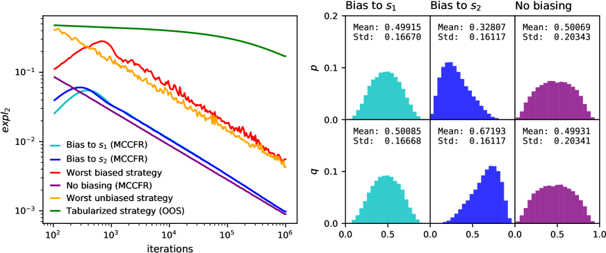
Figure 3: Coordinated Matching Pennies. Left: While individual MCCFR strategies have low exploitability of $\sim 10^{-3}$, the tabularized OOS strategy has high exploitability of $0.17$ after $10^{6}$ iterations. Right: Normalized histograms of probabilities of playing Heads in $s_{1}$ - $p$ and $s_{2}$ - $q$ after $10^{6}$ iterations. The histograms within columns are correlated, as they approximately satisfy equilibrium condition $p+q=1$. Tabularized strategy, combination of $(p,s_{1})$ and $(q,s_{2})$ violates this constraint, resulting in high exploitability.

This simple procedure effectively kick-starts the algorithm to produce distinct trajectories based on $\alpha$.

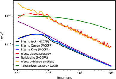
Figure 4: Kuhn Poker

In Figure 3 and in Figure 4 , we show that individual biased strategies converge to Nash equilibria, but the tabularized strategy has higher exploitability even than the worst individual strategy. In CMP, we bias the second player to play in information state $s_{1}$ ($\alpha=0.5$) or $s_{2}$ ($\alpha=1$) information states. In Poker, we bias the first player to play Jack ($\alpha=0$), Queen ($\alpha=1/2$) or King ($\alpha=1$) card. For both experiments, exploration was set to 0.6, biasing to 0.1, and $\mu=500$, a small regret that can be accumulated after less than 500 samples. Within our online framework, the state $\bm{\theta}$ consists of regrets and average strategy accumulators for all information states, and from the state of the pseudo-random number generator, which has distinct initial seeds for each match. The expected strategies are estimated as an average over $3\cdot 10^{4}$ seeds. We plot the worst strategy from these individual biased strategies over all the seeds for all iterations. We plot also MCCFR strategy for reference, to see the influence of biasing and regret initialization.

References

- Brown et al. (2020) Brown, N.; Bakhtin, A.; Lerer, A.; and Gong, Q. 2020. Combining Deep Reinforcement Learning and Search for Imperfect-Information Games. arXiv preprint arXiv:2007.13544 .
- Brown and Sandholm (2017) Brown, N.; and Sandholm, T. 2017. Safe and nested subgame solving for imperfect-information games. In Advances in Neural Information Processing Systems, 689–699.
- Brown and Sandholm (2018) Brown, N.; and Sandholm, T. 2018. Superhuman AI for heads-up no-limit poker: Libratus beats top professionals. Science 359(6374): 418–424.
- Brown and Sandholm (2019) Brown, N.; and Sandholm, T. 2019. Superhuman AI for multiplayer poker. Science 365(6456): 885–890.
- Burch, Johanson, and Bowling (2014) Burch, N.; Johanson, M.; and Bowling, M. 2014. Solving imperfect information games using decomposition. In AAAI, 602–608.
- Campbell, Hoane Jr, and Hsu (2002) Campbell, M.; Hoane Jr, A. J.; and Hsu, F.-h. 2002. Deep blue. Artificial intelligence 134(1-2): 57–83.
- Copeland (2004) Copeland, B. J. 2004. The essential Turing. Clarendon Press.
- Frank and Basin (1998) Frank, I.; and Basin, D. 1998. Search in games with incomplete information: A case study using bridge card play. Artificial Intelligence 100(1-2): 87–123.
- Hoehn et al. (2005) Hoehn, B.; Southey, F.; Holte, R. C.; and Bulitko, V. 2005. Effective short-term opponent exploitation in simplified poker. In AAAI, volume 5, 783–788.
- Kovařík et al. (2019) Kovařík, V.; Schmid, M.; Burch, N.; Bowling, M.; and Lisý, V. 2019. Rethinking formal models of partially observable multiagent decision making. arXiv preprint arXiv:1906.11110 .
- Kuhn (1950) Kuhn, H. W. 1950. A simplified two-person poker. Contributions to the Theory of Games 1: 97–103.
- Lanctot et al. (2009) Lanctot, M.; Waugh, K.; Zinkevich, M.; and Bowling, M. 2009. Monte Carlo sampling for regret minimization in extensive games. In Advances in neural information processing systems, 1078–1086.
- Lisý, Lanctot, and Bowling (2015) Lisý, V.; Lanctot, M.; and Bowling, M. 2015. Online Monte Carlo counterfactual regret minimization for search in imperfect information games. In Proceedings of the 2015 International Conference on Autonomous Agents and Multiagent Systems, 27–36. International Foundation for Autonomous Agents and Multiagent Systems.
- Moravcik et al. (2017) Moravcik, M.; Schmid, M.; Burch, N.; Lisý, V.; Morrill, D.; Bard, N.; Davis, T.; Waugh, K.; Johanson, M.; and Bowling, M. 2017. Deepstack: Expert-level artificial intelligence in heads-up no-limit poker. Science 356(6337): 508–513.
- Osborne and Rubinstein (1994) Osborne, M. J.; and Rubinstein, A. 1994. A course in game theory. MIT press.
- Samuel (1959) Samuel, A. L. 1959. Some studies in machine learning using the game of checkers. IBM Journal of research and development 3(3): 210–229.
- Seitz et al. (2019) Seitz, D.; Kovarík, V.; Lisỳ, V.; Rudolf, J.; Sun, S.; and Ha, K. 2019. Value Functions for Depth-Limited Solving in Imperfect-Information Games beyond Poker. arXiv preprint arXiv:1906.06412 .
- Shannon (1950) Shannon, C. E. 1950. XXII. Programming a computer for playing chess. The London, Edinburgh, and Dublin Philosophical Magazine and Journal of Science 41(314): 256–275.
- Silver et al. (2017) Silver, D.; Schrittwieser, J.; Simonyan, K.; Antonoglou, I.; Huang, A.; Guez, A.; Hubert, T.; Baker, L.; Lai, M.; Bolton, A.; et al. 2017. Mastering the game of go without human knowledge. Nature 550(7676): 354–359.
- Šustr, Kovařík, and Lisý (2019) Šustr, M.; Kovařík, V.; and Lisý, V. 2019. Monte Carlo continual resolving for online strategy computation in imperfect information games. In Proceedings of the 18th International Conference on Autonomous Agents and MultiAgent Systems, 224–232. International Foundation for Autonomous Agents and Multiagent Systems.
- Zinkevich et al. (2008) Zinkevich, M.; Johanson, M.; Bowling, M.; and Piccione, C. 2008. Regret minimization in games with incomplete information. In Advances in neural information processing systems, 1729–1736.