Conway’s drum quilts

Abstract

A ‘transplantable pair’ is a pair of glueing diagrams that can be used to create pairs of plane domains that are isospectral for the Laplace operator. We present a host of transplantable pairs worked out by John Conway using his theory of quilts.

1 Introduction

A ‘transplantable pair’ is a pair of glueing diagrams that can be used to create pairs of plane domains or other spaces that are isospectral for the Laplace operator. The pair is metonymically ‘transplantable’ because isospectrality of the glued spaces can be proven using Peter Buser’s transplantation method, as explained by Buser, Conway, et al. [1] and Conway [3].

John Conway produced a host of transplantable pairs by applying his theory of quilts to small projective groups. I helped by watching admiringly. In this paper I have reproduced his catalog of pairs. The sizes of these pairs are 7, 11, 13, 15, and 21. In [1] we presented the sixteen pairs of sizes 7, 13, and 15, which are treelike and thus give planar isospectral domains. We also presented one of the size 21 pairs, here labeled pair $21(7)$, which yields the ‘homophonic’ domains shown in Figure 1. Conway [4, p. 249] dubbed these domains ‘peacocks rampant and couchant’.

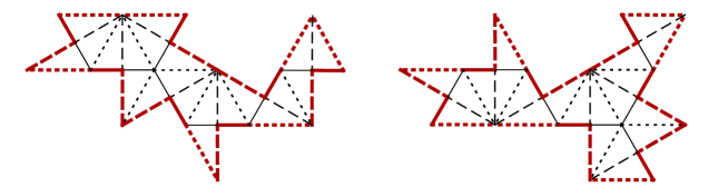
Figure 1: Peacocks rampant and couchant

A transplantable pair can be thought of as arising from a pair of finite permutation actions of the free group on generators $a,b,c$. These actions are equivalent as linear representations but (if the pair is to be of any use) not as permutation representations. In the examples at hand, each representing permutation is an involution, so these representations factor through the quotient $F=\langle a,b,c:a^{2}=b^{2}=c^{2}=1\rangle$, the free product of three copies of the group of order $2$.

From any transplantable pair we can get other pairs through the process of braiding, which amounts to precomposing the permutation representations with automorphisms of $F$, called $L$ and $R$:

$$L:(a,b,c)\mapsto(aba^{-1},a,c);$$

$$R:(a,b,c)\mapsto(a,c,cbc^{-1}).$$

Left-braiding a permutation representation $\rho$ can be viewed as first conjugating $\rho(b)$ by $\rho(a)$, i.e. applying the permutation $\rho(a)$ to each index in the cycle representation of $\rho(b)$, and then switching $\rho(a)$ with the new $\rho(b)$. Right-braiding is the same, only with $c$ taking over the role of $a$.

Pairs of permutations that are equivalent in this way belong to the same quilt. We identify pairs that differ only by permuting $a,b,c$, or by reversing the pair. A quilt has extra structure which we are ignoring here: See Conway and Hsu [5]. This structure makes it easier to understand and enumerate the pairs. But the computer has no trouble churning out all the pairs belonging to the same quilt.

So despite the title and what you might reasonably expect, the only place you will find quilts here is in Appendix A, which reproduces Conway’s original quilt calculations.

First we will present the glueing diagrams, and then the corresponding hyperbolic orbifolds.

2 Transplantation diagrams

In the diagrams that follow, the points being permuted are represented by triangles. The permutations corresponding to $a,b,c$ are represented by lines of three styles: dotted, dashed, and solid. Black lines separate pairs of points that are interchanged by the permutation, while red lines (which are also made thicker) indicate fixed points. Red lines in the interior of the diagram separate points that are each fixed, rather than interchanged. Sometimes black lines occur on the boundary of the diagram, which means that the boundary must be glued up. The computer has taken care to lay out the diagrams so that there is at most one pair of thin boundary lines of each type (dotted, dashed, or solid), so that even without the usual glueing arrows there is no ambiguity of how the boundary is to be glued up.

To refer to these pairs, we will write $7(1)$ for the first pair of quilt 7, $13a(5)$ for the fifth pair of quilt $13a$, etc. This numbering is canonical, given the starting triple $(a,b,c)$, because the quilt has been explored by a ‘left-first search’. More canonical, but more cumbersome, are the Conway symbols of the simplest hyperbolic orbifolds that can be obtained from the pair: See Section 3.

For historical reasons, the four quilts of size 11 are called $11f,11g,11h,11i$. The missing quilts (whose diagrams actually have size 12) are to be found in raw form in Appendix A.

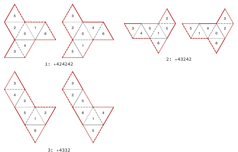
Figure 2: Quilt 7

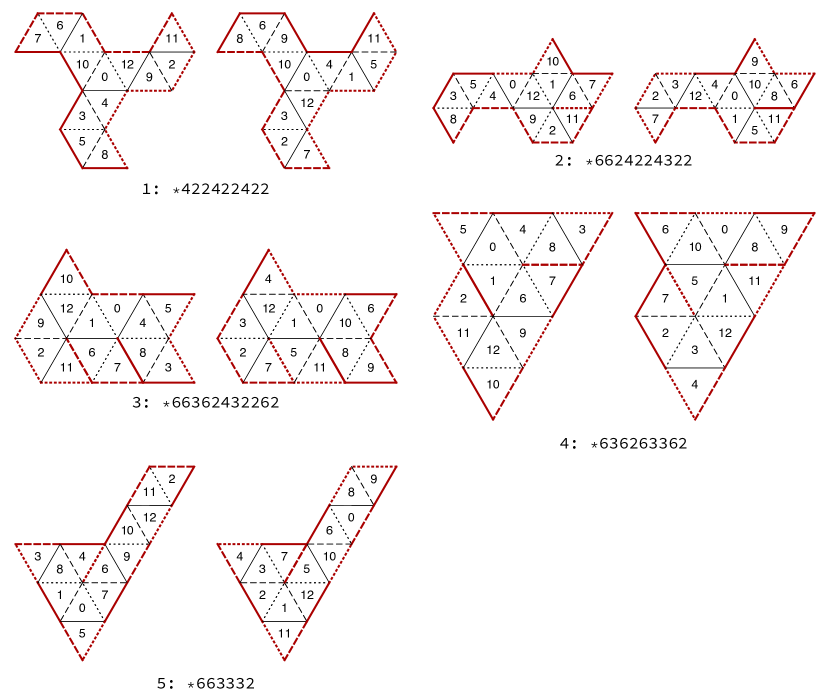
Figure 3: Quilt 13a

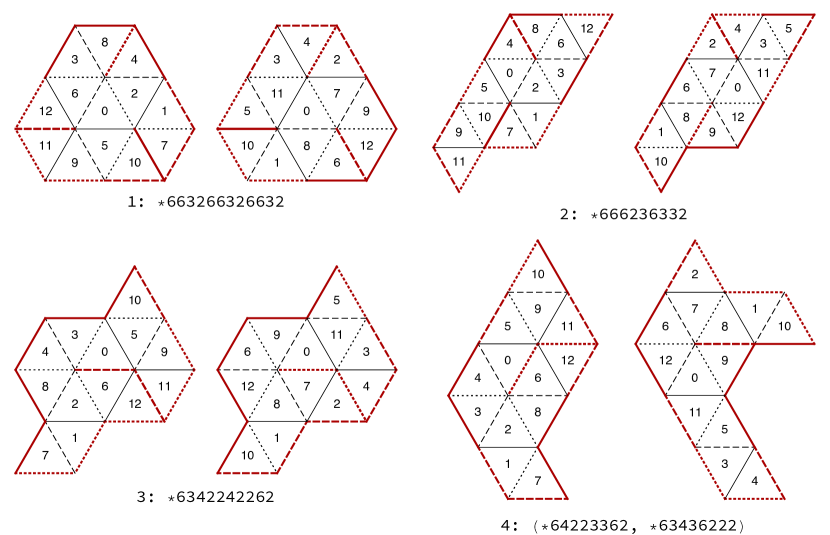
Figure 4: Quilt 13b

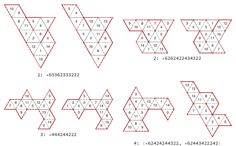
Figure 5: Quilt 15

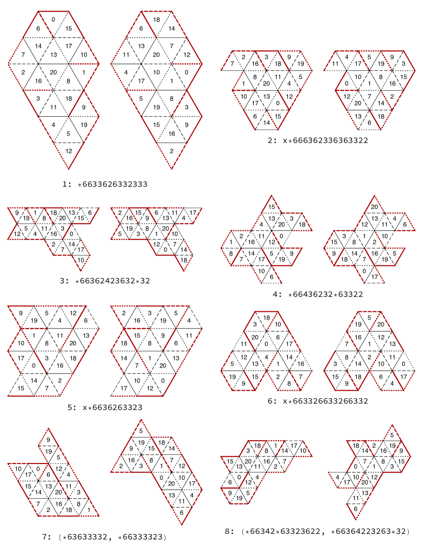
Figure 6: Quilt 21

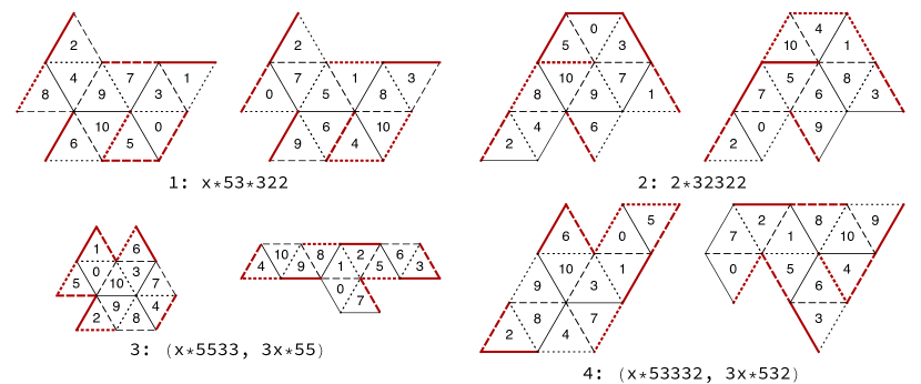
Figure 7: Quilt 11f

Figure 8: Quilt 11g

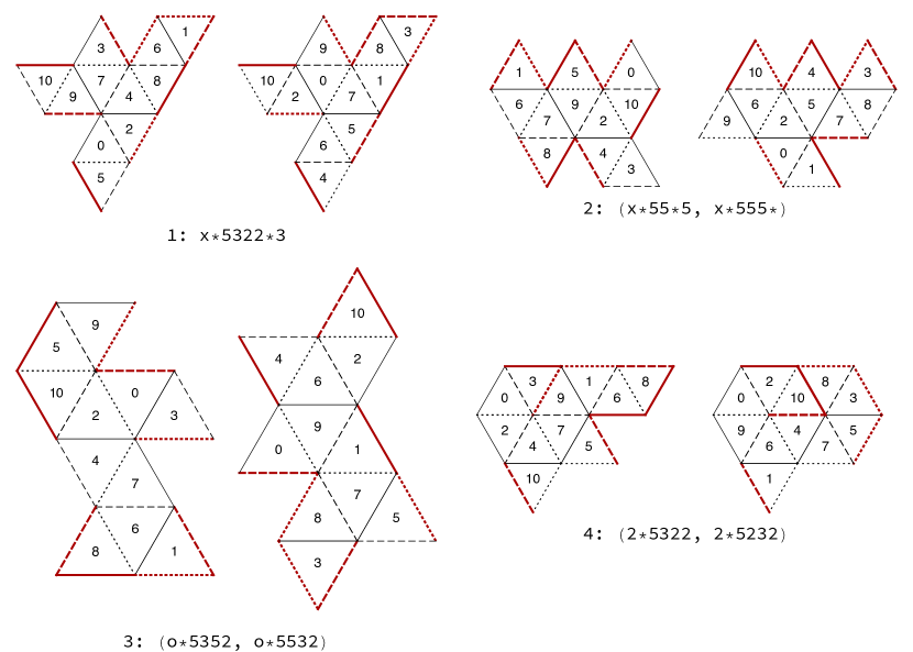
Figure 9: Quilt 11h

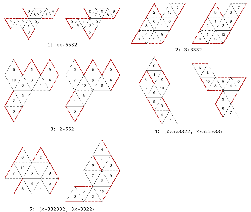
Figure 10: Quilt 11i

3 Hyperbolic orbifolds

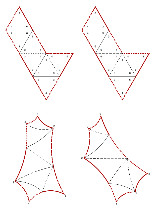
Figure 11: Isospectral hyperbolic hexagons arising from diagram $7(3)$.

Here are the hyperbolic orbifolds corresponding to these transplantable pairs. These are the simplest hyperbolic orbifolds that can be produced using the glueing data. To get them, for the basic triangle we prescribe angles just small enough to make each interior cone point have cone angle evenly dividing $\tau$, and each boundary corner have angle evenly dividing $\tau/2$. When the members of the pair differ only by permuting the labels $a,b,c$, the resulting orbifolds are isometric: To get non-isometric pairs we will need to destroy this symmetry by taking one or more of the triangles smaller. Thus, for example, from the pair $7(3)$ we get the isospectral hexagons shown in Figure 11. This is presumably the simplest pair of isospectral hyperbolic 2-orbifolds.

Each figure gives Conway’s notation (see Conway [2]) for the associated orbifolds.

Note. The pairs show here are isospectral as hyperbolic 2-orbifolds. We can demote an orbifold to a manifold with boundary, and we will still have isospectrality if we impose Neumann boundary conditions. Dirichlet boundary conditions also work, provided that the manifold with boundary is orientable. This will be the case when the diagrams are treelike, or more generally, when all cycles have even length. If there are cycles of odd length, when we put Dirichlet boundary conditions we must also use twisted functions, i.e. sections of a non-trivial bundle, which change sign when you travel around an orientation-reversing path.

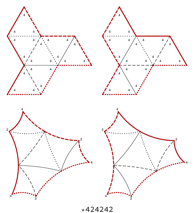
Figure 12: Pair 7(1)

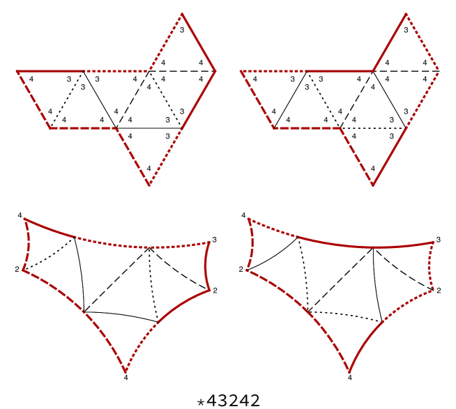
Figure 13: Pair 7(2)

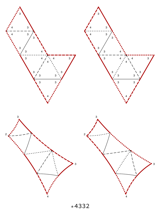
Figure 14: Pair 7(3)

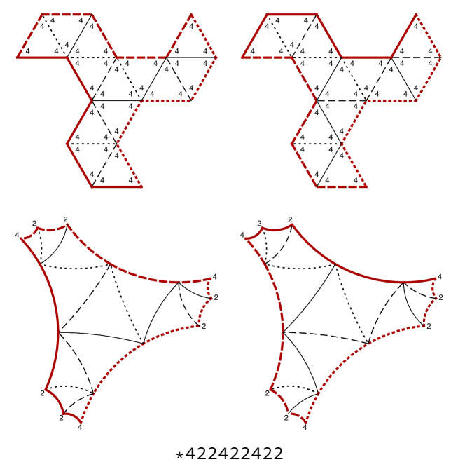
Figure 15: Pair 13a(1)

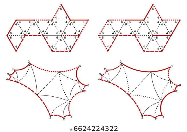
Figure 16: Pair 13a(2)

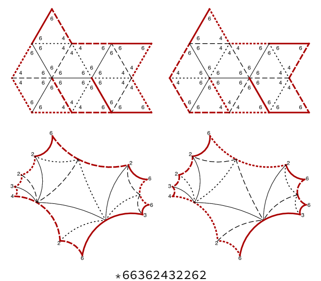
Figure 17: Pair 13a(3)

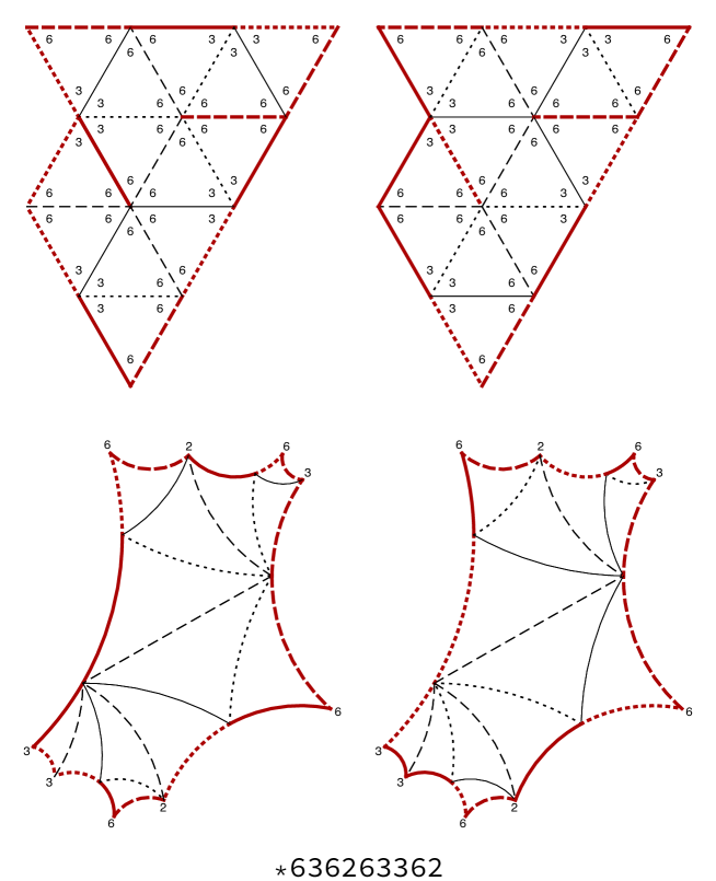
Figure 18: Pair 13a(4)

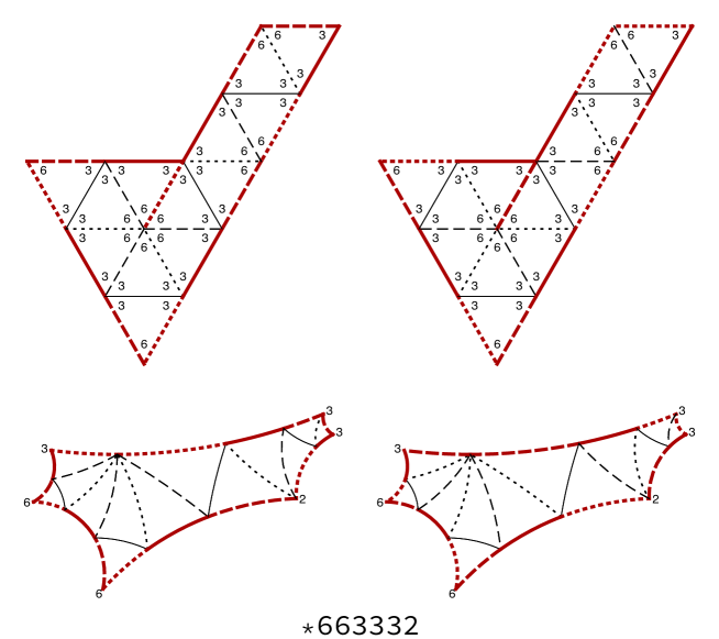
Figure 19: Pair 13a(5)

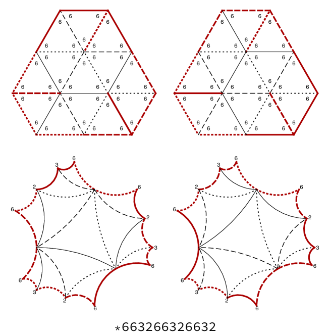
Figure 20: Pair 13b(1)

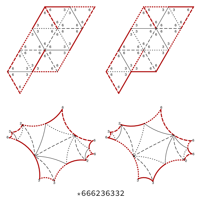
Figure 21: Pair 13b(2)

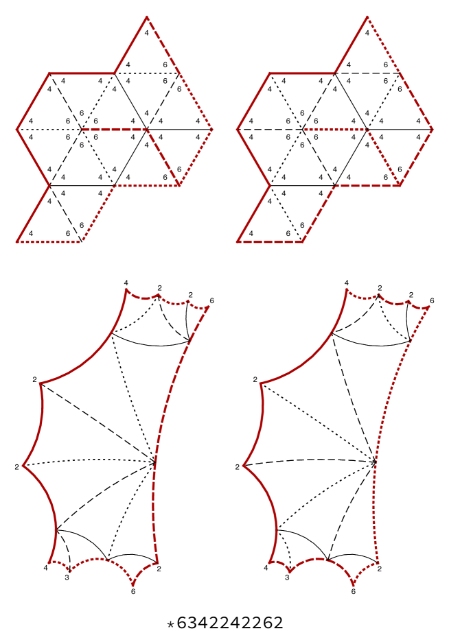
Figure 22: Pair 13b(3)

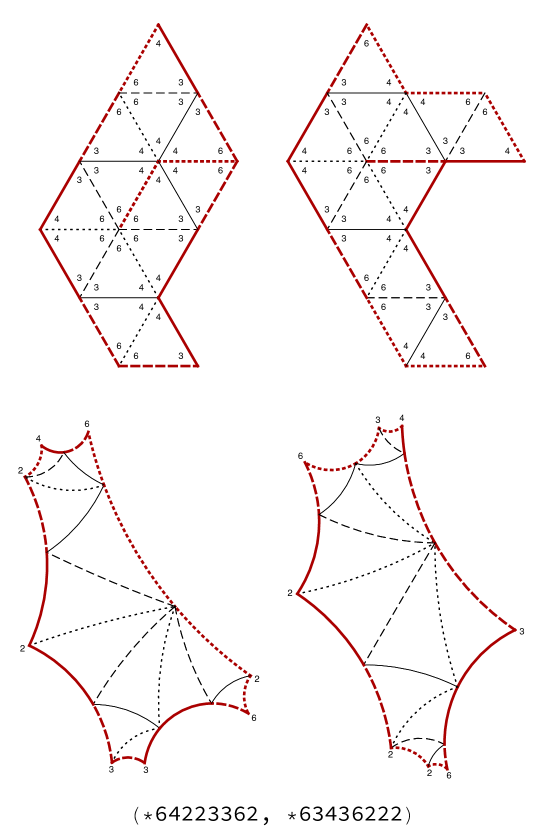
Figure 23: Pair 13b(4)

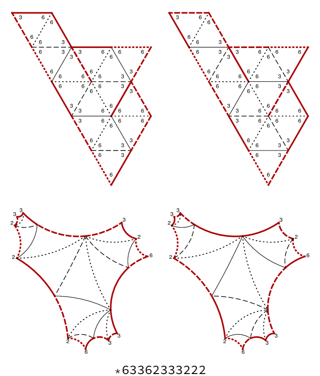
Figure 24: Pair 15(1)

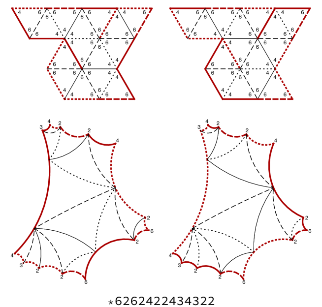
Figure 25: Pair 15(2)

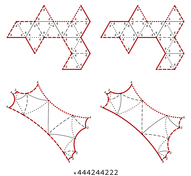
Figure 26: Pair 15(3)

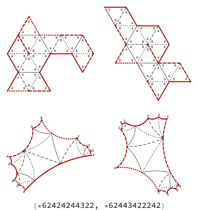
Figure 27: Pair 15(4)

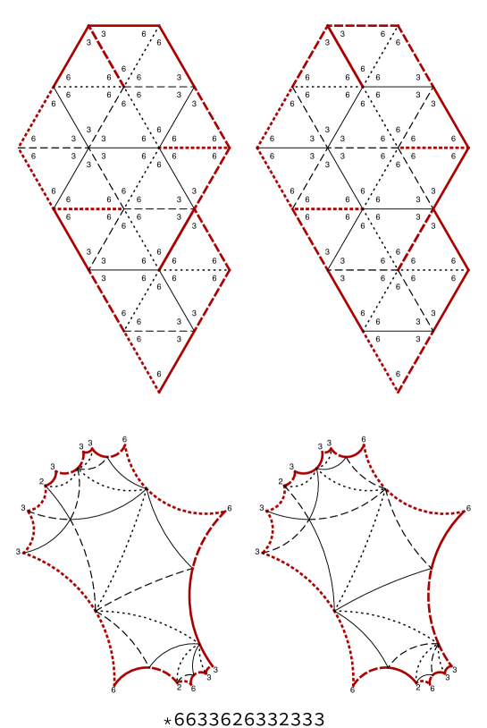
Figure 28: Pair 21(1)

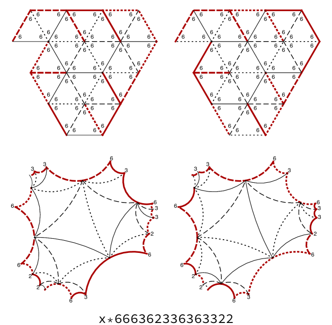
Figure 29: Pair 21(2)

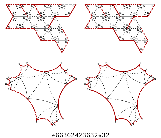
Figure 30: Pair 21(3)

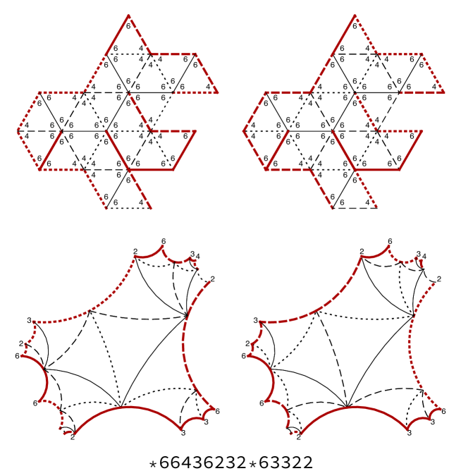
Figure 31: Pair 21(4)

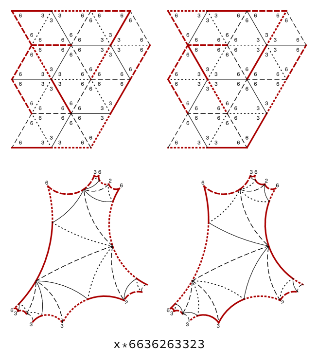
Figure 32: Pair 21(5)

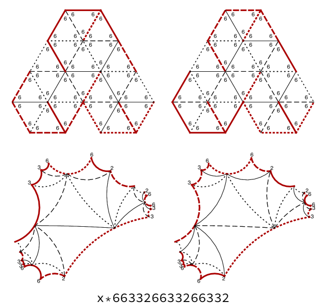
Figure 33: Pair 21(6)

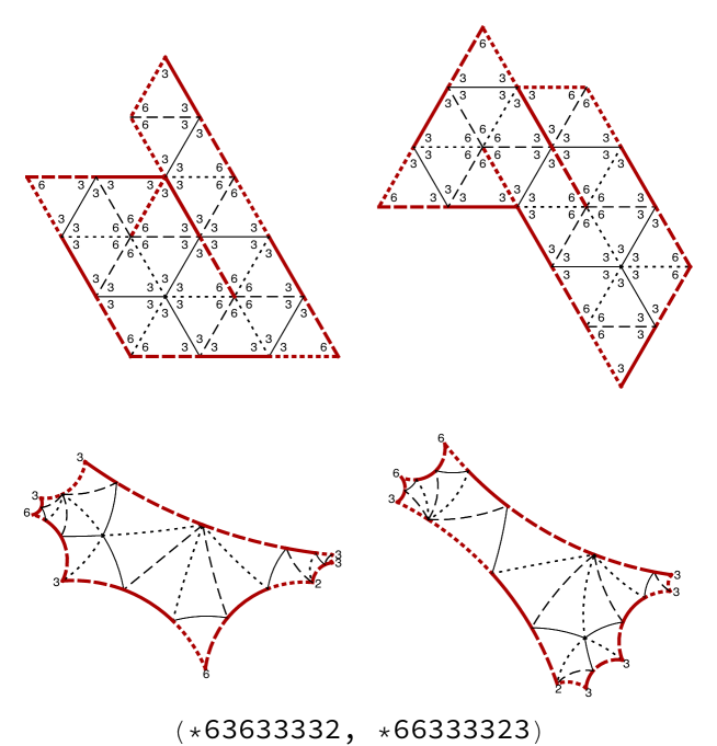
Figure 34: Pair 21(7)

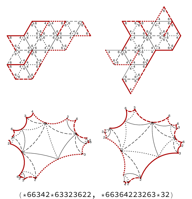
Figure 35: Pair 21(8)

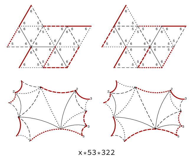
Figure 36: Pair 11f(1)

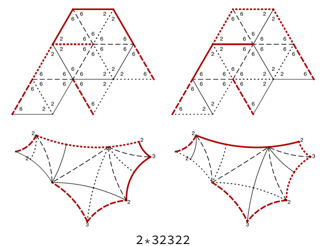
Figure 37: Pair 11f(2)

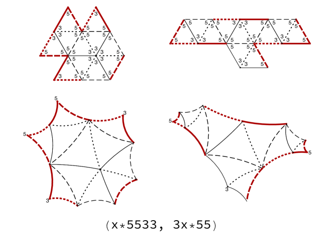
Figure 38: Pair 11f(3)

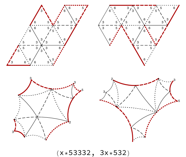
Figure 39: Pair 11f(4)

Figure 40: Pair 11g(1)

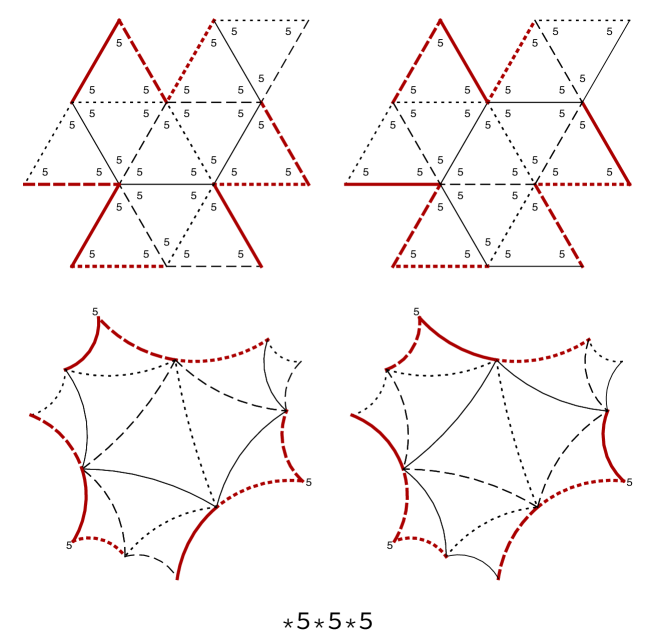
Figure 41: Pair 11g(2)

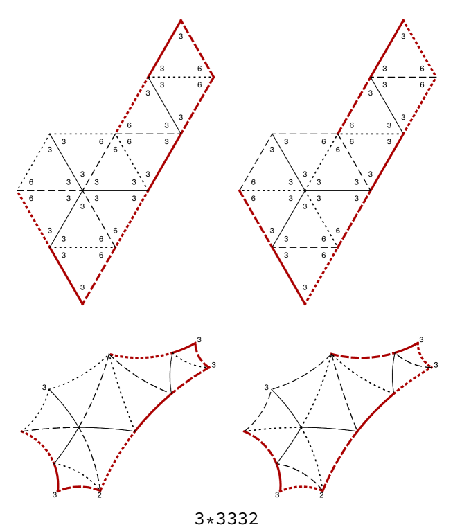
Figure 42: Pair 11g(3)

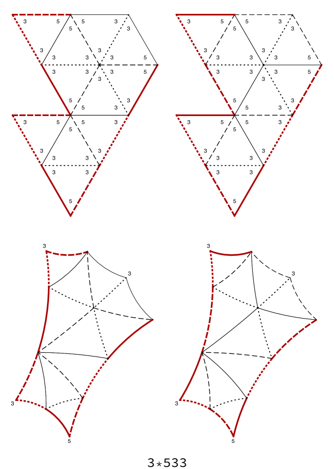
Figure 43: Pair 11g(4)

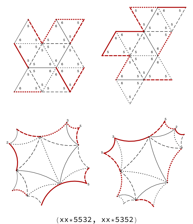
Figure 44: Pair 11g(5)

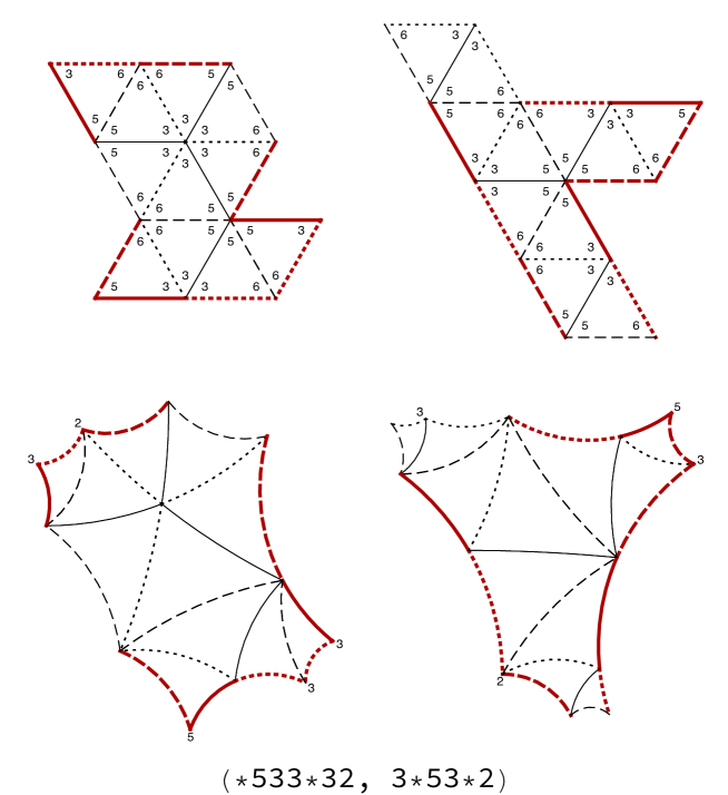
Figure 45: Pair 11g(6)

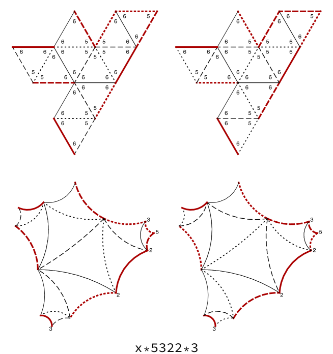
Figure 46: Pair 11h(1)

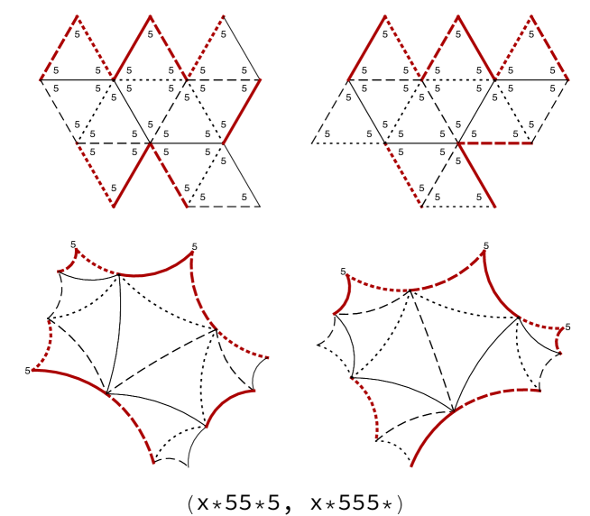
Figure 47: Pair 11h(2)

Figure 48: Pair 11h(3)

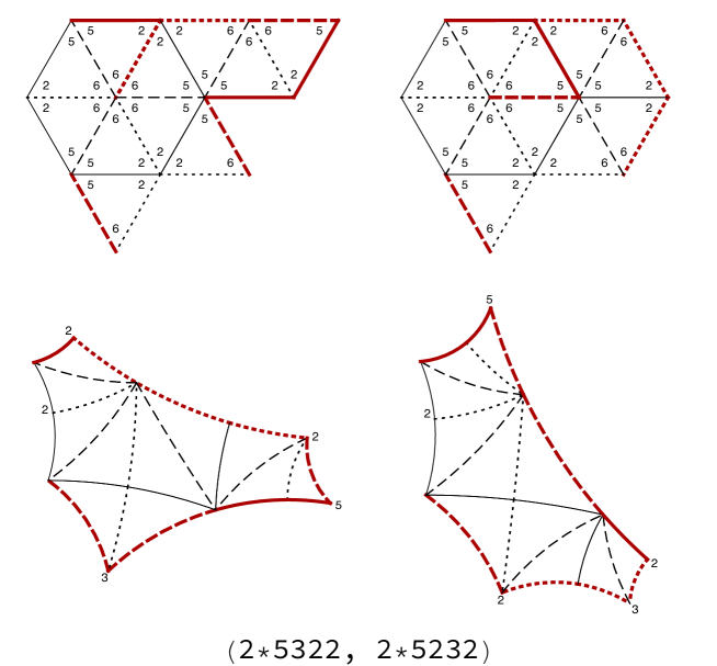
Figure 49: Pair 11h(4)

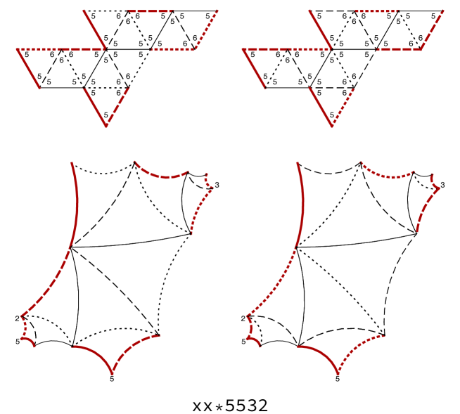
Figure 50: Pair 11i(1)

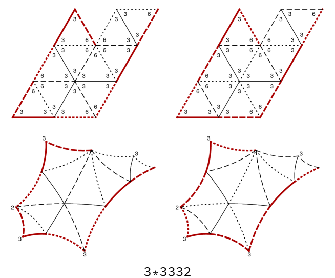
Figure 51: Pair 11i(2)

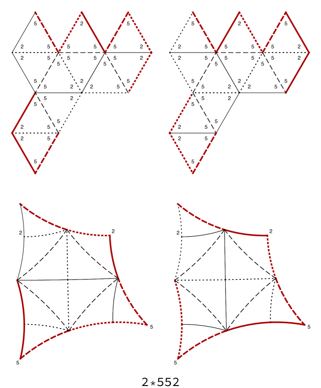
Figure 52: Pair 11i(3)

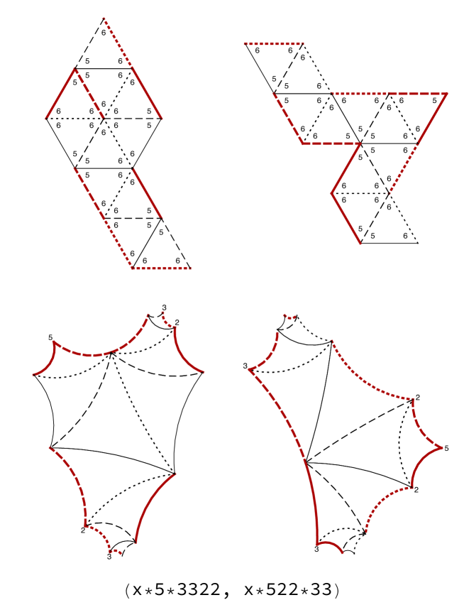
Figure 53: Pair 11i(4)

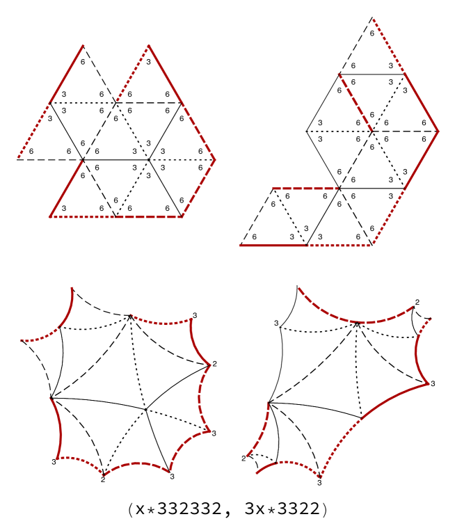
Figure 54: Pair 11i(5)

Appendix A The master at work

Here, in the hand of the master, are quilts, along with associated diagrams for isospectral pairs (including peacocks rampant and couchant in the hand of the pupil).

The 21-octagon map on $\times^{9}$. Octagons are indexed by $\mbox{\small line}_{\mbox{\tiny point on line}}$.

References

- [1] Peter Buser, John Conway, Peter Doyle, and Klaus-Dieter Semmler. Some planar isospectral domains. Internat. Math. Res. Notices, 9, 1994, arXiv:1005.1839v1 [math.DG]. http://arxiv.org/abs/1005.1839v1.
- [2] J. H. Conway. The orbifold notation for surface groups. In Groups, combinatorics & geometry (Durham, 1990), volume 165 of London Math. Soc. Lecture Note Ser., pages 438–447. Cambridge, 1992.
- [3] John H. Conway. The sensual (quadratic) form, volume 26 of Carus Mathematical Monographs. Mathematical Association of America, 1997. With the assistance of Francis Y. C. Fung.
- [4] John. H. Conway, Heidi Burgiel, and Chaim Goodman-Strauss. The Symmetries of Things. Taylor and Francis, 2008.
- [5] John H. Conway and Tim Hsu. Quilts and -systems. J. Algebra, 174(3):856–908, 1995.