Fundamental bound for time measurements and minimum uncertainty clocks

Abstract

We present a simple argument leading to a fundamental minimum uncertainty in the determination of times. It only relies in the uncertainty principle and time dilation in a gravitational field. It implies any attempt to measure times will have a fundamental level of uncertainty. Implications are briefly outlined.

The issue of if the fundamental theories of physics impose limitations on the accuracy of how we can determine physical quantities has been analyzed by several authors over the years. Salecker and Wigner SaWi considered an idealized clock consisting of two mirrors with light bouncing between them and concluded that the minimum uncertainty of such a clock was proportional to the square root of the ratio of the time to be measured and the mass of the clock. Such argument is based exclusively on quantum mechanics. Several authors several have combined that argument with ingredients coming from gravity and reached the conclusion that the clock’s precision has a bound proportional to fractional power of the time to be measured. In particular the fact that one cannot concentrate arbitrarily large quantities of energy in a finite region, as a black hole forms. The constructions require the introduction of several elements, like specific models for clocks or assumptions about the extent of regions of strong gravitational fields. A separate argument by Ng and Lloyd nglloyd uses the Margolus–Levitin theorem and reaches similar conclusions. Here we would like to present a streamlined argument that only relies on the uncertainty principle and the time dilation in gravitational fields and basic error propagation theory to put bounds on the precision of a clock.

The existence of fundamental limitations in the measurements of physical quantities can have profound conceptual implications. For instance, ordinary formulations of quantum mechanics treat time as a classical variable, which implicitly implies that it can be measured with arbitrary precision. Other variables are certainly not treated this way. The limitations in time measurement may lead to a loss of unitarity in the formulation, as variables measured by real clocks cannot track the ideal classical time assumed in the formulation of the Schrödinger equation pedagogical . In fact, limitations on the measurements of space and time have led us to propose a new interpretation of quantum mechanics, the Montevideo Interpretation review .

We here consider a microscopic quantum system playing the role of a clock and a macroscopic observer that interacts with the clock interchanging signals. We start by considering the time-energy uncertainty relation,

$$\Delta E\Delta t_{c}>\hbar.$$ (1)

where $\Delta t_{c}$ is of the order of the period of oscillation of the system being considered. The clock does not necessarily have to be associated to a periodic motion. Busch et al. busch have proposed extensions that allow to consider time as an observable even in the case of non periodic clocks. No matter what type of system we consider, the Helstrom–Holevo bound helstrom sets limits to the measurement of the evolution time of any quantum state. The uncertainty in any estimation of the evolution time of the state through the measurement of an arbitrary observable satisfies the time energy condition.

We now consider the relationship between the time measured by the clock locally, $t_{c}$, and an observer at an infinite distance from it, $t$. The gravitational time dilation was first described by Albert Einstein in 1907 as a consequence of special relativity in accelerated frames of reference. In general relativity, it is considered to be a difference in the passage of proper time at different positions as described by a the metric tensor of space-time. The relevance of this effect in the determination of fundamental limitations to time measurements was emphasized by Frenkel frenkel . It is given by,

$$t=\frac{t_{c}}{\sqrt{1-\frac{r_{S}}{r}}},$$ (2)

with $r_{S}$ the Schwarzschild radius of the clock in question, $r_{s}=2GE/c^{4}$ with $E$ the energy of the clock and $r$ its radius. We will assume that an observer cannot be arbitrarily close to the clock. For a standard atomic clock this effect may seem negligible but for an optimal clock it would be important as we shall see. The best clocks we can consider are quantum systems that are microscopic. In such a case an observer will not be able to get close to the clock, and its distance, for all practical purposes can be taken to be infinite (at least compared to the microscopic value of $r$).

As an example, take an atomic clock based on the transition of an electron between energy levels in an atom. We construct an electromagnetic source at the frequency that maximizes the probability that an electron transition between levels. This is a frequency standard. The source emits photons that interact with the atom and make the electron transition. We repeat this for many atoms and check how many are excited. This allows to maximize the transition probability. In reality the photon, after being emitted, falls in the gravitational field of the atom, allowing to use (2) to compute the red shift of the photon’s frequency. There is an uncertainty in the frequency of the emitted photon. This uncertainty will suffer the correction due to time dilation described above. Nowadays, the best clocks we have taken as reference are based on low energy atomic transitions. It would be desirable to have transitions of higher frequency, but stability presents an experimental challenge. We are neglecting other possible quantum gravitational effects since we are considering processes that always occur in clocks larger than their Schwarzschild radius, and we will encode the fluctuations of the metric in the uncertainties of the Schwarzschild radius.

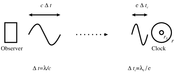
Figure 1: A schematic description of the setup

We would like to establish the uncertainty in the observed period of oscillation. Using the standard technique for the propagation of errors of a measurement, taking differentials of the above expression, we have that,

$$\left(\Delta t\right)^{2}=\frac{1}{4}\frac{t_{c}^{2}\left(\Delta r_{S}\right)^{2}}{\left(1-\frac{r_{S}}{r}\right)^{3}r^{2}}+\frac{\left(\Delta t_{c}\right)^{2}}{{1-\frac{r_{S}}{r}}},$$ (3)

and from the definition of the Schwarzschild radius,

$$\left(\Delta r_{S}\right)^{2}=\frac{4G^{2}\left(\Delta E\right)^{2}}{c^{8}},$$ (4)

and therefore for the clock that minimizes the uncertainty $\Delta t$ the following holds,

$$\Delta r_{S}=\frac{4G^{2}\hbar^{2}}{c^{8}\left(\Delta t_{c}\right)^{2}}.$$ (5)

And substituting (5) in (3), we get,

$$\left(\Delta t\right)^{2}=\frac{t_{c}^{2}G^{2}\hbar^{2}}{\left(1-\frac{r_{S}}{r}\right)^{3}r^{2}c^{8}\Delta t_{c}^{2}}+\frac{\left(\Delta t_{c}\right)^{2}}{1-\frac{r_{S}}{r}},$$ (6)

this indicates that $\Delta t_{c}$ will be bounded since it appears in the numerator and the denominator. We observe that $1-r_{S}/r$ is a positive quantity less than one, since the size of the clock cannot be smaller than its Schwarzschild radius, and using (2) to translate $t_{c}$ to $t$, one has that,

$$\left(\Delta t\right)^{2}=\frac{t_{c}^{2}G^{2}\hbar^{2}}{\left(1-\frac{r_{S}}{r}\right)^{3}r^{2}c^{8}\left(\Delta t_{c}\right)^{2}}+\frac{\left(\Delta t_{c}\right)^{2}}{1-\frac{r_{S}}{r}}>\frac{t^{2}G^{2}\hbar^{2}}{r^{2}c^{8}\left(\Delta t_{c}\right)^{2}}+\left(\Delta t_{c}\right)^{2},$$ (7)

and assuming that the clock has size $r$ and that the oscillation within it takes place at the mean speed $v$ we have that $2\pi r=v\Delta t_{c}$. Then, differentiating with respect to $\Delta t_{c}$ to find the minimum value of the time uncertainty and get, that the minimum occurs at,

$$\Delta t_{c}=\frac{\sqrt{2}\pi^{1/3}c^{1/3}\left(t^{2}t_{\rm Planck}^{4}\right)^{1/6}}{v^{1/3}},$$ (8)

with $l_{\rm Planck}$ Planck’s length. This expression is minimized when $v$ is the speed of light, yielding,

$$\Delta t_{c}=\sqrt{2}\pi^{1/3}\left(tt_{\rm Planck}^{2}\right)^{1/3},$$ (9)

with $t_{\rm Planck}$ Planck’s time, and this corresponds to a value of the error in the observed time of

$$\Delta t>\sqrt{3}\pi^{1/3}t^{1/3}t_{\rm Planck}^{2/3}.$$ (10)

This bound depends on $t$, for $t=1$ second is ten orders of magnitude smaller than the accuracy of the best current clocks, $\Delta t/t$ is smaller the larger the time $t$. One can also estimate $\Delta E/E$, which turns out to be smaller than $10^{-20}$ for the measurement of a one second interval and decreases as the interval to be measured increases. Using equation (2) it can be easily seen that this bound is saturated by a clock with a radius approximately given by $r=3r_{S}$.

This limit is similar to the ones obtained by previous authors but it did not assume any particular model of the clock, only the uncertainty principle and the formula for time dilation in a gravitational field. It also suggests, taking into account equations (2), (9) and (10), what is the ideal clock, a clock that saturates the bound, an oscillation given by a particle orbiting the black hole near $3r_{S}$, the innermost stable circular orbit of a non-rotating black hole. It might be possible to go beyond that with orbits at slightly lower radius, respecting the bound of equation (10), but it would be difficult to create a stable system.

Summarizing, it is possible to obtain a bound for the accuracy reachable by a clock using only fundamental bounds of quantum mechanics and taking into account the gravitational time dilation without having to go into the details of the practical implementation of the clock. The analysis is interpretation independent.

We thank an anonymous referee for bringing the Helstrom–Holevo bound argument to our attention. This work was supported in part by Grants NSF-PHY-1603630, NSF-PHY-1903799, funds of the Hearne Institute for Theoretical Physics, CCT-LSU, Pedeciba and Fondo Clemente Estable FCE_1_2019_1_155865.

References

- (1) H.Salecker, E.P.Wigner:, Phys. Rev. 109, 571 (1958).
- (2) F. Karolyhazy, Nuo. Cim. A42, 390 (1966); Y. J. Ng, H. van Dam, Mod. Phys. Lett. A9, 335(1994); Ann. N. Y. Acad. Sci 755, 579 (1995); G. Amelino-Camelia, Mod. Phys. Lett. A9, 3415 (1994).
- (3) Y. J. Ng, S. Lloyd, Sci. Am. 291, 53 (2004)
- (4) R. Gambini, R. Porto and J. Pullin, Gen. Rel. Grav. 39, 1143 (2007) doi:10.1007/s10714-007-0451-1 [gr-qc/0603090].
- (5) R. Gambini and J. Pullin, Entropy 20, no. 6, 413 (2018) doi:10.3390/e20060413 [arXiv:1502.03410 [quant-ph]].
- (6) P. Busch, M. Grabovski, P .J. Lahti, “Operational quantum physics”. Lect. Notes Phys. m31, Springer (1997).
- (7) A. Montanaro, Prof. IEEE Information Theory Workshop, 378 (2008) [arXiv:0711.2012]; S. L. Braunstein, C. M. Caves, and G. J. Milburn, Annals of Physics 247, 135 (1996); A. S. Holevo, Probabilistic and Statistical Aspects of Quantum Theory (North-Holland, Amsterdam, 1982).
- (8) A. Frenkel, Found. Phys. 45, no. 12, 1561 (2015).