Exact travelling wave solutions in viscoelastic channel flow

Abstract

Elasto-inertial turbulence (EIT) is a new, two-dimensional chaotic flow state observed in polymer solutions with possible connections to inertialess elastic turbulence and drag-reduced Newtonian turbulence. In this Letter, we argue that the origins of EIT are fundamentally different from Newtonian turbulence by finding a dynamical connection between EIT and an elasto-inertial linear instability recently found at high Weissenberg numbers (Garg et al. Phys. Rev. Lett. 121, 024502, 2018). This link is established by isolating the first known exact coherent structures in viscoelastic parallel flows - nonlinear elasto-inertial travelling waves (TWs) - borne at the linear instability and tracking them down to substantially lower Weissenberg numbers where EIT exists. These TWs have a distinctive “arrowhead’ structure in the polymer stretch field and can be clearly recognised, albeit transiently, in EIT, as well as being attractors for EIT dynamics if the Weissenberg number is sufficiently large. Our findings suggest that the dynamical systems picture in which Newtonian turbulence is built around the co-existence of many (unstable) simple invariant solutions populating phase space carries over to EIT, though these solutions rely on elasticity to exist.

The addition of only a few parts per million of long chain polymer molecules to a Newtonian solvent can fundamentally alter classical (Newtonian) turbulence at high Reynolds number ($Re\gg 1$, White and Mungal (2008)) and seed new, visually striking chaotic motion in viscosity-dominated flows, which persist even in the inertialess limit ($Re\ll 1$) – so-called elastic turbulence Groisman and Steinberg (2000). The disruption of near-wall Newtonian turbulence is well known due to the accompanied reduction in skin-friction drag (up to 80%) and is exploited in oil pumping, for example in the trans-Alaska pipeline. For the fluid’s elasticity to manifest, the Weissenberg number ($Wi$, the ratio between a polymer relaxation timescale and a flow timescale) must be large enough to allow the polymers to stretch as they are sheared, creating an elastic tension in the streamlines. In drag-reduced flows, this effect seems to reduce the sweeps of high-momentum fluid towards the wall, though the exact mechanisms of polymeric drag reduction, and the universality of its maximum drag reduction (MDR) at 80% Virk (1970); Graham (2014) remain open research questions.

Recently, experiments and simulations have revealed the existence of a new turbulent flow state observed at modest inertia and elasticity ($Re=O(1000)$, $Wi=O(10)$, Samanta et al. (2013); Dubief et al. (2013)). This elasto-inertial turbulence (EIT) is dominated by spanwise-coherent sheets in which the polymer becomes highly stretched, and attached to the sheets are regions of intense rotational and extensional flow Dubief et al. (2013); Terrapon et al. (2014). Recent numerical simulations have confirmed that EIT is a two-dimensional phenomenon Sid et al. (2018), while experiments in pipe flow indicate that MDR may be a feature of EIT and not a polymeric perturbation of Newtonian turbulence Choueiri et al. (2019) as has been assumed Xi and Graham (2012). Very recently, numerical simulations of EIT have revealed the existence of a recurring coherent structure in the turbulence - an ‘arrowhead’ of polymer stretch - upon which EIT collapses as the Weissenberg number is increased Dubief et al. (2020). The potential importance of EIT in drag reduced flows – and also a possible link to elastic turbulence at $Re=0$ – raises the important question as to its origin. One candidate is a newly-discovered elasto-inertial instability Garg et al. (2018), found in planar channel flow and pipe flow, but which exists at much higher $Wi$ than those at which EIT has been observed. The linearly unstable eigenfunctions of the instability also bear little resemblence to the recently found ‘arrowhead’ state seen in EIT making any link unclear.

The purpose of this Letter is to establish this link by demonstrating that the elasto-inertial travelling waves which originate at the bifurcation point found by Garg et al. Garg et al. (2018) correspond to the arrowhead coherent structures found in EIT Dubief et al. (2020). Specifically, we show that: a) this bifurcation is substantially subcritical in $Wi$ so states connected with the instability exist at much lower $Wi$ where EIT exists; and b) it is the upper branch of travelling waves which correspond to the arrowhead solutions not the far weaker lower branch states which resemble the eigenfunctions. Beyond the significance of isolating exact nonlinear structures in viscoelastic channel flows for the first time, our findings suggest (as conjectured by Garg et al. Garg et al. (2018)) that EIT is built around the nonlinear states which originate at an elasto-inertial instability in a similar manner to Newtonian turbulence, albeit with a completely different bifurcation structure of underlying elasto-inertial states.

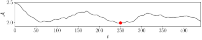
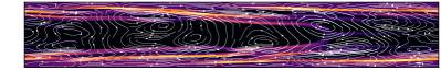
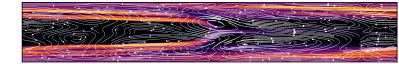
Figure 1: (Top) Time evolution of volume-averaged trace of the polymer conformation relative to the laminar value, $\mathcal{A}:=\langle\text{tr}\mathbf{C}\rangle_{V}/\langle\text{tr}\mathbf{C}_{\text{lam}}\rangle_{V}$, in a computation of EIT in a long domain, $l_{x}=4\pi$, at $Re=1000$, $Wi=20$. (Middle) Snapshot of the flow extracted at $t=250$ (see marker in the top panel), contours show $\text{tr}\mathbf{C}/L^{2}$, lines are the perturbation streamfunction for ($\mathbf{u}-\mathbf{U}_{\text{lam}}$). (Bottom) Snapshot of transient EIT at $Wi=30$, with all other parameters held fixed. The flow here eventually settles onto a stable travelling wave (an arrowhead).

Direct numerical simulations (DNS) are performed in a 2D channel under conditions of constant mass-flux using the FENE-P model,

$$\partial_{t}\mathbf{u}+\mathbf{u}\cdot\boldsymbol{\nabla}\mathbf{u}+\boldsymbol{\nabla}p =\frac{\beta}{Re}\nabla^{2}\mathbf{u}+\frac{(1-\beta)}{Re}\boldsymbol{\nabla}\cdot\mathbf{T},$$ (1a)

$$\boldsymbol{\nabla}\cdot\mathbf{u} =0,$$ (1b)

$$\partial_{t}\mathbf{C}+\mathbf{u}\cdot\boldsymbol{\nabla}\mathbf{C}+\mathbf{T} =\mathbf{C}\cdot\boldsymbol{\nabla}\mathbf{u}+(\boldsymbol{\nabla}\mathbf{u})^{T}\cdot\mathbf{C}$$ (1c)

where the polymeric stress, $$\mathbf{T} \mathbf{C}$$, is related to the polymer conformation tensor, , via the Peterlin function

$$\mathbf{T}=\frac{1}{Wi}\left(\frac{\mathbf{C}}{1-\text{tr}\mathbf{C}/L^{2}}-\mathbf{I}\right).$$ (1d)

The equations are non-dimensionalised by the channel half height, $h$, and bulk velocity $U_{b}$, so the Reynolds and Weissenberg numbers are defined as $Re:=hU_{b}/\nu$ and $Wi:=\tau U_{b}/h$ with $\tau$ the polymer relaxation time. The ratio of solvent to total viscosities, $\beta:=\nu_{s}/\nu$, is fixed at $\beta=0.9$ and the maximum extension of the polymer chains relative to their equilibrium length is held at $L=500$. The numerical method uses second-order finite differences in both directions which ensures the discrete conservation of mass, momentum and kinetic energy, has been extensively validated and described in detail in Sid et al. (2018).

A Newton-Krylov solver is wrapped around the DNS code to converge travelling waves (TWs) as exact solutions of the governing equations. A global diffusion term $\nabla^{2}\mathbf{C}/ReSc$ is added to the right hand side of (1dc) with a Schmidt number of $Sc=10^{3}$ as in Sid et al. (2018). The presence of this global diffusion dramatically improves convergence properties in the Newton solver, and we obtain qualitatively similar results when timestepping the TWs with this term removed (i.e. $Sc=\infty$). Computation and continuation of travelling waves are performed in a box of streamwise length $l_{x}=\pi$ at a usual resolution $N_{x}=128$, $N_{z}=513$ (others were used to check robustness) with calculations in longer boxes done with correspondingly higher stereamwise resolution to retain the same grid spacing $\Delta x$.

The time evolution of the volume-averaged trace of $\mathbf{C}$ in a long-box ($l_{x}=4\pi$) calculation at $(Re,Wi)=(1000,20)$ is reported in figure 1, alongside a representative snapshot of the flow. The attractor in this configuration is chaotic, and the flow shows features common to earlier computations of EIT, including the arrangement of strong regions of $\text{tr}\mathbf{C}$ in thin sheets which orient and stretch in the direction of the driving flow. Notable in the snapshot is the presence of the large “arrowhead” structure (about 3/4 along the channel) , which is roughly symmetric about the channel centreline and consists of a pair of sheets which reach down into the near wall regions but also curve up to meet at $z=0$. As shown in the lower panel of figure 1, the arrowhead becomes more pronounced with increasing $Wi$ (it is a stable attractor at $Wi=30$). The emergence and stabilisation of arrowheads with increasing $Wi$ has been examined recently in Dubief et al. (2020); they appear to be fundamental structures underpinning EIT. We now show how arrowheads connect to the centre mode instability discovered in Garg et al. (2018).

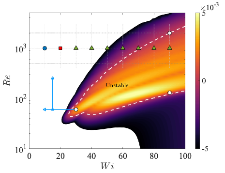
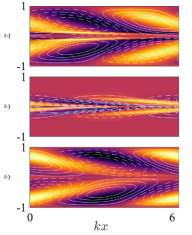
Figure 2: (Left) Contours of linear growth rate $\sigma$ for most unstable symmetric instability waves in a two-dimensional channel flow of a FENE-P fluid ($L=500$) for streamwise wavenumbers $k\in\mathbb{N}$. The dashed white line indicates marginal stability $\sigma=0$. The overlayed grid and symbols identify DNS runs in a box of length $l_{x}=2\pi$: (blue circle) laminar, (red square) EIT, (green triangle) arrowhead. The blue lines identify where we have performed arclength continuation of the nonlinear travelling wave born in this instability (at $k=2$). (Right) Visualisation of the instability wave in the $x-z$ plane at points indicated by white circles in the stability diagram. Contours show the trace of the (perturbation) conformation, lines the streamfunction. From top to bottom: $(Re,Wi,k)=(60,30,2)$, $(2000,90,7)$ and $(130,90,1)$.

Linear stability results for the centre mode instability are reported in figure 2. These results were obtained by linearising equations (1d) and solving for the complex frequency $\omega=\omega_{r}+\mathrm{i}\sigma$ of normal mode perturbations $\boldsymbol{\varphi}(\mathbf{x},t)=\hat{\boldsymbol{\varphi}}(z)\text{exp}(\mathrm{i}kx-\mathrm{i}\omega t)$, where $\boldsymbol{\varphi}\equiv(u,w,{\rm c}_{xx},{\rm c}_{xz},{\rm c}_{zz},p)$ is a vector of the flow variables. Since computations are performed in boxes of length $l_{x}=m\pi$ with $m\in\mathbb{N}$, we search over integer wavenumbers only. The resulting temporal eigenvalue problem was solved by expanding in $N_{c}\sim 200$ Chebyshev polynomials over half the channel, $z\in[-1,0]$, and applying symmetry conditions at $z=0$ ($u$ symmetric, $w$ antisymmetric).

The centre mode first becomes unstable at $(Re,Wi,k)\sim(50,25,2)$; the associated eigenfunction (also shown in figure 2) consists of trains of tilted vortices of opposite sign either side of $z=0$. On the upper branch of the $\sigma=0$ curve, the instability moves to increasingly high wavenumbers and becomes localized at the channel centreline (for more on the scalings in pipe flow see Garg et al. (2018)).

We have conducted a number of complementary DNS calculations in a box of length $l_{x}=2\pi$ at $Re=1000$ in which we attempt to trigger EIT by applying suction and blowing at the walls (see Dubief et al., 2013; Sid et al., 2018); the results are overlayed on the stability diagram in figure 2. The calculations include a large region of parameter space where the flow is predicted to be linearly stable, and EIT is obtained for modest $Wi$ prior to the emergence and stabilisation of a single domain-filling arrowhead structure (either steady or weakly periodic in time) as $Wi$ increases. In regions of instability, the attractor is always an arrowhead, which would be consistent with a connection to the linear bifurcation. However, the $k=1$ mode is stable in all the parameter configurations used in the DNS calculations, clearly implying subcriticality.

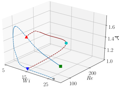
Figure 3: Arclength continuation in $Wi$ at $Re=60$ (blue) and in $Re$ at $Wi=15$ (maroon) in a box of length $l_{x}=\pi$. The amplitude $\mathcal{A}:=\langle\text{tr}\mathbf{C}\rangle_{V}/\langle\text{tr}\mathbf{C}_{\text{lam}}\rangle_{V}$. The solution curve was initialised at $(Re,Wi)=(60,30)$ by perturbing a laminar flow with the linear instability wave at $k=2$, which was allowed to saturate onto the stable upper branch solution. The saddle node at $Re=60$ is at $Wi=8.77$; the saddle node at $Wi=15$ is at $Re=253.71$. The linear bifurcation point at $(Re,Wi)=(60,26.9)$ is identified with a small black circle. Snapshots of the the TW at points highlighted on the curve are shown in figure 4.

To substantiate the connection of the arrowhead solution to the centre mode bifurcation and show the bifurcation’s significant subcritical nature, we take the centre mode eigenfunction just beyond the point of marginal stability, $(Re,Wi,k)=(60,30,2)$, and apply it as a perturbation to the laminar flow in a $l_{x}=\pi$ box. Timestepping leads to saturation onto a stable TW which shares some similarity to the linearised eigenfunction, although with a conformation field which is significantly perturbed (note the amplitude in figure 3 and the snapshot of the TW in figure 4). The TW readily converges in a Newton solver looking for a steady solution in a Galilean frame and then can be arclength-continued around in $Wi$ while holding $Re$ fixed: see figure 3. The amplitude of the travelling wave initially increases as $Wi$ drops with a saddle node bifurcation reached at $Wi\approx 8.8$ and a (very) low amplitude lower branch connects back to the bifurcation point at $Wi\approx 26.9$. The upper branch TW has a Hopf bifurcation at $Wi\approx 20$ below which the attractor is a simple (relative) periodic orbit with period $T=O(100)$ ($T\sim 250$ at $Wi=15$) and the TW restabilises at $Wi\approx 10$.

The structure of the (unstable) TW at the subcritical pair $(Re,Wi)=(60,15)$ is shown in figure 4 for both the upper and lower branches. On the upper branch, resemblance to the linear stability wave is largely lost and the $\text{tr}\mathbf{C}$ field has adopted the arrowhead form: a single curved sheet of highly stretched polymer runs across the channel centreline (compare with the structure in the $l_{x}=4\pi$ domain of figure 1) and the flow field is mirror symmetric about $z=0$. The lower branch state does not resemble the arrowhead and is somewhat closer to the linear eigenfunction, although there is a pair of weak sheets of polymer stretch clearly visible.

To probe the connection of the arrowhead emerging from the centre mode bifurcation to EIT, we also take the TW at $Wi=15$ and continue up in $Re$: see the maroon curve in figure 3. The TW is unstable up to $Re\approx 115$ – whether the periodic orbit exists subcritically beyond this point has not yet been investigated. At this $Wi$, the saddle node sits at $Re\approx 254$ where, again, the state takes the shape of an arrowhead in polymer stretch: see figure 4. The sheets either side of the centreline have moved inwards relative to their position at $Re=60$, though this movement is not monotonic with increasing $Re$.

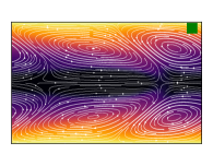
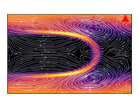
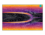
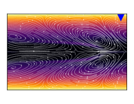
Figure 4: Travelling waves corresponding to points identified in figure 3. Contours show $\text{tr}\mathbf{C}/L^{2}$, lines are the perturbation ($\mathbf{u}-\mathbf{U}_{\text{lam}}$) streamfunction. The aspect ratio matches the snapshot of the long domain ($l_{x}=4\pi$) calculation reported in figure 1.

Further work is required to establish the self-sustaining mechanism that produces the arrowhead, though the parameter values for which it is observed indicate that elasto-inertial wave propagation along tensioned streamlines may play a role (see the linear mechanisms discussed in Page and Zaki (2015, 2016)); this may also help to establish the $z$-locations of the parallel sheets of polymer stretch that make up the ‘edges’ of the arrowhead. Other recent studies have argued for the importance of structures connected to Newtonian Tollmien-Schlichting (TS) waves Shekar et al. (2019) in EIT, but have not been able to explicitly continue these TWs around in the parameter space. These studies have been performed at much higher Reynolds numbers and higher values of the solvent viscosity than those considered here. Continuation of both the arrowhead and TS TWs in longer boxes will help establish where these dynamics overlap.

In summary, we have isolated the first exact coherent structures in viscoelastic channel flow by performing arclength continuation from the recently discovered high-$Wi$ instability reported in Garg et al. (2018). Our computations have demonstrated that the bifurcation is strongly subcritical in both $Wi$ and $Re$. The upper branch solutions take the form of large arrowhead structures in the polymer stress field – structures which are observed intermittently in computations of EIT in large boxes and which have been observed to be stable attractors at very high $Wi$. Beyond indicating that the origins of EIT are purely elastic in nature and so disconnected from Newtonian dynamics, more importantly, these exact coherent structures provide a crucial beachhead to identify the self-sustaining processes which underpin EIT and also possible connections to elastic turbulence.

References

- White and Mungal (2008) C. M. White and M. G. Mungal, “Mechanics and prediction of turbulent drag reduction with polymer additives,” Annual Review of Fluid Mechanics 40, 235–256 (2008).
- Groisman and Steinberg (2000) A. Groisman and V. Steinberg, “Elastic turbulence in a polymer solution flow,” Nature 405, 53–55 (2000).
- Virk (1970) P. S. Virk, “Drag reduction fundamentals,” AIChE Journal 21, 625–656 (1970).
- Graham (2014) M. D. Graham, “Drag reduction and the dynamics of turbulence in simple and complex fluids,” Physics of Fluids 26, 101301 (2014).
- Samanta et al. (2013) D. S. Samanta, Y. Dubief, H. Holzner, C. Schäfer, A. N. Morozov, C. Wagner, and B. Hof, “Elasto-inertial turbulence,” Proceedings of the National Academy of Sciences of the United States of America 110, 10557–10562 (2013).
- Dubief et al. (2013) Y. Dubief, V. E. Terrapon, and J. Soria, “On the mechanism of elasto-inertial turbulence.” Physics of Fluids 25, 110817 (2013).
- Terrapon et al. (2014) V. E. Terrapon, Y. Dubief, and J. Soria, “On the role of pressure in elasto-inertial turbulence,” Journal of Turbulence 16, 26–43 (2014).
- Sid et al. (2018) S. Sid, V. E. Terrapon, and Y. Dubief, “Two-dimensional dynamics of elasto-inertial turbulence and its role in polymer drag reduction,” Physical Review Fluids 3, 01130(R) (2018).
- Choueiri et al. (2019) G. H. Choueiri, J. M. Lopez, and B. Hof, “Exceeding the Asymptotic Limit of Polymer Drag Reduction§,” Physical Review Letters 120, 124501 (2019).
- Xi and Graham (2012) L. Xi and M. D. Graham, “Intermittent dynamics of turbulence hibernation in Newtonian and viscoelastic minimal channel flows,” Journal of Fluid Mechanics 693, 433–472 (2012).
- Dubief et al. (2020) Y. Dubief, J. Page, R. R. Kerswell, V. E. Terrapon, and V. Steinberg, “A first coherent structure in elasto-inertial turbulence,” arXiv 2006.06770 (2020).
- Garg et al. (2018) P. Garg, I. Chaudhary, M. Khalid, V. Shankar, and G. Subramanian, “Viscoelastic Pipe Flow is Linearly Unstable,” Physical Review Letters 121, 024502 (2018).
- Page and Zaki (2015) J. Page and T. A. Zaki, “The dynamics of spanwise vorticity perturbations in homogeneous viscoelastic shear flow,” Journal of Fluid Mechanics 777, 327–363 (2015).
- Page and Zaki (2016) J. Page and T. A. Zaki, “Viscoelastic shear flow over a wavy surface,” Journal of Fluid Mechanics 801, 392–429 (2016).
- Shekar et al. (2019) A. Shekar, R. M. McMullen, S. Wang, B. J. McKeon, and M. D. Graham, “Critical-Layer Structures and Mechanisms in Elastoinertial Turbulence,” Physical Review Letters 122, 124503 (2019).