A Multi-Agent Primal-Dual Strategy for Composite Optimization over Distributed Features

Abstract

This work studies multi-agent sharing optimization problems with the objective function being the sum of smooth local functions plus a convex (possibly non-smooth) function coupling all agents. This scenario arises in many machine learning and engineering applications, such as regression over distributed features and resource allocation. We reformulate this problem into an equivalent saddle-point problem, which is amenable to decentralized solutions. We then propose a proximal primal-dual algorithm and establish its linear convergence to the optimal solution when the local functions are strongly-convex. To our knowledge, this is the first linearly convergent decentralized algorithm for multi-agent sharing problems with a general convex (possibly non-smooth) coupling function.

I Introduction

We consider $K$ agents connected through a graph. Each agent can only send and receive information from its immediate neighbors. Its goal is to find its corresponding solution, denoted by $w^{\star}_{k}\in{\mathbb{R}}^{Q_{k}}$, of the following coupled multi-agent optimization problem:

$$\min_{w_{1},\cdots,w_{K}}\quad\sum_{k=1}^{K}J_{k}(w_{k})+g\Big{(}\sum_{k=1}^{K}B_{k}w_{k}\Big{)},$$ (1)

where the smooth function $J_{k}:{\mathbb{R}}^{Q_{k}}\rightarrow{\mathbb{R}}$ and the matrix $B_{k}\in{\mathbb{R}}^{E\times Q_{k}}$ are known by agent $k$ only, and $g:{\mathbb{R}}^{E}\rightarrow{\mathbb{R}}\cup\{+\infty\}$ is a convex possibly non-smooth function known by all agents. Problem (1) is the sharing formulation, where the agents own different variables but are coupled through the function $g$. Problems of the form (1) appear in many machine learning applications, such as regression over distributed features [1, 2], dictionary learning over distributed models [3], and clustering in graphs [4]. They also appear in engineering applications, including smart grid control [5] and network utility maximization [6]. For a general convex function $g$, centralized algorithms for (1) have been shown to achieve global linear convergence if the matrix $[B_{1},\cdots,B_{K}]$ has full row rank and $\sum\limits_{k=1}^{K}J_{k}(w_{k})$ is strongly-convex [7, 8, 9]. On the other hand, decentralized algorithms have only been shown to converge linearly under stricter conditions than centralized ones. In this work, we aim toward closing the gap in linear convergence between centralized and decentralized algorithms for problem (1).

Literature Review. Sharing problems have been studied in different fields and date back to studies in economics [10] –see the discussion in [1]. The earliest center-free algorithm to solve such problems dates back to [11]. Decentralized solutions for the sharing formulation (1) have only been shown to achieve global linear convergence for special cases and under stricter conditions compared to the centralized ones as we now explain. The works [12, 13, 14, 15] establish linear convergence for resource allocation formulations, where $g$ is an indicator function of zero (i.e., $g(x)=0$ if $x=0$ and $\infty$ otherwise) and $B_{k}=I$, for smooth and strongly-convex local costs. The work [16] also establishes linear convergence for resource allocation problems in the presence of simple local constraints (i.e., $\underline{w}\leq w_{k}\leq\overline{w}$), but under stronger assumptions on the costs such as twice differentiability of $J_{k}$ and knowledge of the conjugate function of $J_{k}$. The works [17, 18] establish linear convergence for special cases with $g$ being an indicator function of zero; moreover, each $B_{k}$ is required to have full row rank in [17] or satisfy a certain rank condition in [18]. The works [19, 20] establish linear convergence for strongly convex objectives and a smooth coupling function $g$.

Note that problem (1) recovers the consensus problem [21, 22, 23] if we choose $g$ such that it returns zero when $w_{1}=\cdots=w_{K}$ and $\infty$ otherwise. In this case, the matrix $B=[B_{1},\cdots,B_{K}]$ is sparse and encodes the communication graph between agents. The works [24, 25, 26] studied linear convergence of consensus problems in the presence of a common non-smooth term, which is not applicable for the sharing problem. Different from the consensus problem, the matrix $B$ in the sharing problem is not necessarily sparse, and $B_{k}$ is a private matrix known by agent $k$ only. Thus, solution methods for these two problems are different [1]. To the best of our knowledge, establishing linearly convergent algorithms for the sharing problem (1) with a general convex $g$ are still missing.

Contribution. As mentioned before, there is a theoretical gap between centralized and decentralized algorithms for the sharing problem (1). In this work, we propose a decentralized algorithm for (1) and establish its linear convergence to the global solution. The derivation of our algorithm is based on reformulating (1) into an equivalent problem that is amenable to decentralized solutions. This technique motivates the derivation of many other decentralized algorithms.

Notation. We let $\|x\|^{2}_{D}=x^{\mathsf{T}}Dx$ for a square matrix $D$. The symbol $I_{S}$ denotes the identity matrix of size $S$, and $S$ is removed when there is no confusion. The symbol $\mathds{1}_{N}$ denotes the $N\times 1$ vector with all entries being one. The Kronecker product of two matrices is denoted by $A\otimes B$. We use ${\mathrm{c}ol}\{x_{k}\}_{k=1}^{K}$ to denote a column vector formed by stacking $x_{1},\cdots,x_{K}$ on top of each other and $\text{blkdiag}\{X_{k}\}_{k=1}^{K}$ to denote a block diagonal matrix consisting of diagonal blocks $\{X_{k}\}$. The subdifferential $\partial f(x)$ of a function $f$ at $x$ is the set of all subgradients. The proximal operator of a function $f(x)$ with step-size $\mu$ is ${\mathrm{p}rox}_{\mu f}(x)=\operatorname*{arg\,min}\limits_{u}\ f(u)+{1\over 2\mu}\|x-u\|^{2}$. The conjugate of a function $f$ is defined as $f^{*}(v)=\sup\limits_{x}\ v^{\mathsf{T}}x-f(x)$. A differentiable function $f$ is $\delta$-smooth and $\nu$-strongly-convex if $\|{\nabla}f(x)-{\nabla}f(y)\|\leq\delta\|x-y\|$ and $(x-y)^{\mathsf{T}}\big{(}{\nabla}f(x)-{\nabla}f(y)\big{)}\geq\nu\|x-y\|^{2}$, respectively, for any $x$ and $y$.

II Saddle-Point Reformulation

In this section, we provide the main assumption on the objective and explain how (1) is reformulated into an equivalent saddle-point problem. We introduce the quantities:

$${\scriptstyle{\mathcal{W}}} \;\stackrel{{\scriptstyle\Delta}}{{=}}\;{\mathrm{c}ol}\{w_{1},\cdots,w_{K}\}\in{\mathbb{R}}^{Q},~{}Q\textstyle\;\stackrel{{\scriptstyle\Delta}}{{=}}\;\sum_{k=1}^{K}Q_{k},$$ (2a)

$${\mathcal{J}}({\scriptstyle{\mathcal{W}}}) \;\stackrel{{\scriptstyle\Delta}}{{=}}\;\textstyle\sum_{k=1}^{K}J_{k}(w_{k}),$$ (2b)

$$B \;\stackrel{{\scriptstyle\Delta}}{{=}}\;\begin{bmatrix}B_{1}&\cdots&B_{K}\end{bmatrix}\in{\mathbb{R}}^{E\times Q}.$$ (2c)

Then, problem (1) can be rewritten as:

$$\min_{{\scriptstyle{\scalebox{0.5}{\mbox{$\displaystyle\mathcal{W}$}}}}}\quad{\mathcal{J}}({\scriptstyle{\mathcal{W}}})+g\left(B{\scriptstyle{\mathcal{W}}}\right).$$ (3)

Throughout this work, the following assumption holds.

Assumption 1.

(Objective Functions) Problem (3) has a solution ${\scriptstyle{\mathcal{W}}}^{\star}$, and the function ${\mathcal{J}}:{\mathbb{R}}^{Q}\rightarrow{\mathbb{R}}$ is $\delta$-smooth and $\nu$-strongly-convex with $0<\nu\leq\delta$. Moreover, the function $g:{\mathbb{R}}^{E}\rightarrow{\mathbb{R}}\cup\{+\infty\}$ is proper lower semi-continuous and convex, and there exists ${\scriptstyle{\mathcal{W}}}\in{\mathbb{R}}^{Q}$ such that $B{\scriptstyle{\mathcal{W}}}$ belongs to the relative interior domain of $g$.

Under Assumption 1, strong duality holds [27, Corollary 31.2.1], and problem (3) is equivalent to the following saddle-point problem [28, Proposition 19.18]:

$$\boxed{\min_{{\scriptstyle{\scalebox{0.5}{\mbox{$\displaystyle\mathcal{W}$}}}}}\max_{y}\quad{\mathcal{J}}({\scriptstyle{\mathcal{W}}})+y^{\mathsf{T}}B{\scriptstyle{\mathcal{W}}}-g^{*}(y)}$$ (4)

where $y$ is the dual variable and $g^{*}$ is the conjugate function of $g$. A primal-dual pair $({\scriptstyle{\mathcal{W}}}^{\star},y^{\star})$ is optimal if, and only if, it satisfies the optimality conditions [28, Proposition 19.18]:

$$-B^{\mathsf{T}}y^{\star} ={\nabla}{\mathcal{J}}({\scriptstyle{\mathcal{W}}}^{\star}),$$ (5a)

$$B{\scriptstyle{\mathcal{W}}}^{\star} \in\partial g^{*}(y^{\star}).$$ (5b)

Directly solving (4) does not result in a decentralized algorithm. This is because the dual variable $y$ couples all agents, and these algorithms would require a centralized unit to compute the dual update. Therefore, further reformulations are needed to derive a decentralized solution.

III Decentralized Reformulation

In this section, we reformulate (4) into another equivalent saddle-point problem that can be solved in a decentralized manner. Since the dual variable $y$ couples all agents, we introduce local copies of $y$ at all agents. Let $y_{k}$ denote a local copy of $y$ at agent $k$. In addition, we introduce the following network quantities:

$${\scriptstyle{\mathcal{Y}}} \;\stackrel{{\scriptstyle\Delta}}{{=}}\;{\mathrm{c}ol}\{y_{k}\}_{k=1}^{K}\in{\mathbb{R}}^{EK},\quad{\mathcal{G}}^{*}({\scriptstyle{\scalebox{0.7}{\mbox{$\displaystyle\mathcal{Y}$}}}})\;\stackrel{{\scriptstyle\Delta}}{{=}}\;{1\over K}\sum_{k=1}^{K}g^{*}(y_{k}),$$

$${\mathcal{B}}_{d} \;\stackrel{{\scriptstyle\Delta}}{{=}}\;{\mathrm{b}lkdiag}\{B_{k}\}_{k=1}^{K}\in{\mathbb{R}}^{EK\times Q},$$

and the symmetric matrix ${\mathcal{L}}\in{\mathbb{R}}^{EK\times EK}$ such that:

$${\mathcal{L}}{\scriptstyle{\mathcal{Y}}}=0\iff y_{1}=\cdots=y_{K}.$$ (7)

Consider the saddle-point problem:

$$\boxed{\min_{{\scriptstyle{\scalebox{0.5}{\mbox{$\displaystyle\mathcal{W}$}}}},{\scriptstyle{\scalebox{0.7}{\mbox{$\displaystyle\mathcal{X}$}}}}}\max_{{\scriptstyle{\scalebox{0.7}{\mbox{$\displaystyle\mathcal{Y}$}}}}}\quad{\mathcal{J}}({\scriptstyle{\mathcal{W}}})+{\scriptstyle{\scalebox{0.7}{\mbox{$\displaystyle\mathcal{Y}$}}}}^{\mathsf{T}}{\mathcal{B}}_{d}{\scriptstyle{\mathcal{W}}}+{\scriptstyle{\scalebox{0.7}{\mbox{$\displaystyle\mathcal{Y}$}}}}^{\mathsf{T}}{\mathcal{L}}{\scriptstyle{\scalebox{0.7}{\mbox{$\displaystyle\mathcal{X}$}}}}-{\mathcal{G}}^{*}({\scriptstyle{\mathcal{Y}}})}$$ (8)

with an optimal solution $({\scriptstyle{\mathcal{W}}}^{\star},{\scriptstyle{\scalebox{0.7}{\mbox{$\displaystyle\mathcal{X}$}}}}^{\star},{\scriptstyle{\scalebox{0.7}{\mbox{$\displaystyle\mathcal{Y}$}}}}^{\star})$ satisfying [28]:

$$-{\mathcal{B}}_{d}^{\mathsf{T}}{\scriptstyle{\mathcal{Y}}}^{\star} ={\nabla}{\mathcal{J}}({\scriptstyle{\mathcal{W}}}^{\star}),$$ (9a)

$${\mathcal{L}}{\scriptstyle{\mathcal{Y}}}^{\star} =0,$$ (9b)

$${\mathcal{B}}_{d}{\scriptstyle{\mathcal{W}}}^{\star}+{\mathcal{L}}{\scriptstyle{\scalebox{0.7}{\mbox{$\displaystyle\mathcal{X}$}}}}^{\star} \in\partial{\mathcal{G}}^{*}({\scriptstyle{\mathcal{Y}}}^{\star}).$$ (9c)

Problem (8) can be solved in a decentralized manner because the matrix ${\mathcal{L}}$ encodes the network sparsity structure and the matrix ${\mathcal{B}}_{d}$ is block diagonal. We now show that problems (8) and (4) are equivalent.

Lemma 1.

(Saddle-Point) If $({\scriptstyle{\mathcal{W}}}^{\star},{\scriptstyle{\scalebox{0.7}{\mbox{$\displaystyle\mathcal{X}$}}}}^{\star},{\scriptstyle{\scalebox{0.7}{\mbox{$\displaystyle\mathcal{Y}$}}}}^{\star})$ satisfies the optimality condition (9), then it holds that ${\scriptstyle{\mathcal{Y}}}^{\star}=\mathds{1}_{K}\otimes y^{\star}$ with $({\scriptstyle{\mathcal{W}}}^{\star},y^{\star})$ satisfying the optimality condition (5).

Proof.

From equations (7) and (9b), we have that ${\scriptstyle{\mathcal{Y}}}^{\star}=\mathds{1}_{K}\otimes y^{\star}$ for some $y^{\star}$. Thus, equation (9a) can be written as:

$$-{\mathcal{B}}_{d}^{\mathsf{T}}{\scriptstyle{\mathcal{Y}}}^{\star}=-B^{\mathsf{T}}y^{\star}={\nabla}{\mathcal{J}}({\scriptstyle{\mathcal{W}}}^{\star}).$$ (10)

Multiplying (9c) by $\mathds{1}_{K}^{\mathsf{T}}\otimes I_{E}$ and using ${\scriptstyle{\mathcal{Y}}}^{\star}=\mathds{1}_{K}\otimes y^{\star}$ gives:

$$(\mathds{1}_{K}^{\mathsf{T}}\otimes I_{E}){\mathcal{B}}_{d}{\scriptstyle{\mathcal{W}}}^{\star}+(\mathds{1}_{K}^{\mathsf{T}}\otimes I_{E}){\mathcal{L}}{\scriptstyle{\scalebox{0.7}{\mbox{$\displaystyle\mathcal{X}$}}}}^{\star} \in(\mathds{1}_{K}^{\mathsf{T}}\otimes I_{E})\partial{\mathcal{G}}^{*}({\scriptstyle{\mathcal{Y}}}^{\star})$$

$$\Longrightarrow B{\scriptstyle{\mathcal{W}}}^{\star}\in\partial g^{*}(y^{\star}),$$ (11)

where we used the fact that $(\mathds{1}_{K}^{\mathsf{T}}\otimes I_{E}){\mathcal{L}}=0$, which holds from (7). From equations (10) and (11), we see that $({\scriptstyle{\mathcal{W}}}^{\star},y^{\star})$ satisfies the optimality condition (5). ∎

IV Decentralized Strategy

In this section, we propose an algorithm to solve (8) and show how to implement it in a decentralized manner.

IV-A General Algorithm

Let ${\scriptstyle{\mathcal{W}}}_{-1},{\scriptstyle{\mathcal{Y}}}_{-1}$ be any values and ${\scriptstyle{\scalebox{0.7}{\mbox{$\displaystyle\mathcal{X}$}}}}_{-1}=0$. The iteration is:

$${\scriptstyle{\mathcal{W}}}_{i} ={\scriptstyle{\mathcal{W}}}_{i-1}-\mu_{w}{\nabla}{\mathcal{J}}({\scriptstyle{\mathcal{W}}}_{i-1})-\mu_{w}{\mathcal{B}}^{\mathsf{T}}_{d}{\scriptstyle{\mathcal{Y}}}_{i-1},$$ (12a)

$${\scriptstyle{\scalebox{0.85}{\mbox{$\displaystyle\mathcal{Z}$}}}}_{i} ={\scriptstyle{\mathcal{Y}}}_{i-1}+\mu_{y}{\mathcal{B}}_{d}{\scriptstyle{\mathcal{W}}}_{i}+{\mathcal{L}}{\scriptstyle{\scalebox{0.7}{\mbox{$\displaystyle\mathcal{X}$}}}}_{i-1},$$ (12b)

$${\scriptstyle{\scalebox{0.7}{\mbox{$\displaystyle\mathcal{X}$}}}}_{i} ={\scriptstyle{\scalebox{0.7}{\mbox{$\displaystyle\mathcal{X}$}}}}_{i-1}-{\mathcal{L}}{\scriptstyle{\scalebox{0.85}{\mbox{$\displaystyle\mathcal{Z}$}}}}_{i},$$ (12c)

$${\scriptstyle{\mathcal{Y}}}_{i} ={\mathrm{p}rox}_{\mu_{y}{\mathcal{G}}^{*}}(\bar{{\mathcal{A}}}{\scriptstyle{\scalebox{0.85}{\mbox{$\displaystyle\mathcal{Z}$}}}}_{i}),$$ (12d)

where $\bar{{\mathcal{A}}}=\bar{A}\otimes I_{E}$ with $\bar{A}\in{\mathbb{R}}^{K\times K}$ satisfying Assumption 2.

Assumption 2.

(Combination Matrices) We assume that $\bar{A}$ is a primitive symmetric doubly-stochastic matrix. Moreover, we assume that the matrix ${\mathcal{L}}$ satisfies condition (7) and

$$0<I-{\mathcal{L}}^{2},\quad\bar{{\mathcal{A}}}^{2}\leq I-{\mathcal{L}}^{2}.$$ (13)

The condition on $\bar{A}$ can be easily satisfied for any undirected connected network – see [23]. Note that the eigenvalues of $\bar{{\mathcal{A}}}$ belong to $(-1,1]$. Given $\bar{{\mathcal{A}}}$, there are many choices for ${\mathcal{L}}$. For instance, we can let ${\mathcal{L}}^{2}=I-\bar{{\mathcal{A}}}^{2}$ and check whether $I-{\mathcal{L}}^{2}$ is positive definite or not. If it is positive definite, then the assumption is satisfied. If not, we can let ${\mathcal{L}}^{2}=c(I-\bar{{\mathcal{A}}}^{2})$ for any $c\in(0,1)$. Although many choices for ${\mathcal{L}}$ and $\bar{\mathcal{A}}$ are possible, due to space considerations, we only focus on one choice in this work.

We first construct a primitive symmetric doubly-stochastic matrix $A=[a_{sk}]\in{\mathbb{R}}^{K\times K}$ such that $a_{sk}=0$ if two agents $s$ and $k$ are not connected through an edge. Then, we let $\bar{A}=0.5(I+A)$, which is also a primitive symmetric doubly-stochastic matrix. In this case, the eigenvalues of $\bar{\mathcal{A}}$ belong to $(0,1]$, and we can let ${\mathcal{L}}^{2}=I-\bar{\mathcal{A}}$, which satisfies Assumption 2. We now show how to implement (12) using these choices.

IV-B Proximal Exact Dual Diffusion (PED²)

From (12b)–(12c), it holds that, for all $i\geq 1$,

$${\scriptstyle{\scalebox{0.85}{\mbox{$\displaystyle\mathcal{Z}$}}}}_{i} =(I-{\mathcal{L}}^{2}){\scriptstyle{\scalebox{0.85}{\mbox{$\displaystyle\mathcal{Z}$}}}}_{i-1}+{\scriptstyle{\mathcal{Y}}}_{i-1}-{\scriptstyle{\mathcal{Y}}}_{i-2}+\mu_{y}{\mathcal{B}}_{d}({\scriptstyle{\mathcal{W}}}_{i}-{\scriptstyle{\mathcal{W}}}_{i-1}).$$ (14)

It eliminates ${\scriptstyle{\scalebox{0.7}{\mbox{$\displaystyle\mathcal{X}$}}}}_{i}$, and we can rewrite (12) as

$${\scriptstyle{\mathcal{W}}}_{i} ={\scriptstyle{\mathcal{W}}}_{i-1}-\mu_{w}{\nabla}{\mathcal{J}}({\scriptstyle{\mathcal{W}}}_{i-1})-\mu_{w}{\mathcal{B}}^{\mathsf{T}}_{d}{\scriptstyle{\mathcal{Y}}}_{i-1},$$

$${\scriptstyle{\scalebox{0.85}{\mbox{$\displaystyle\mathcal{Z}$}}}}_{i} =(I-{\mathcal{L}}^{2}){\scriptstyle{\scalebox{0.85}{\mbox{$\displaystyle\mathcal{Z}$}}}}_{i-1}+{\scriptstyle{\mathcal{Y}}}_{i-1}-{\scriptstyle{\mathcal{Y}}}_{i-2}+\mu_{y}{\mathcal{B}}_{d}({\scriptstyle{\mathcal{W}}}_{i}-{\scriptstyle{\mathcal{W}}}_{i-1}),$$

$$\phi_{i} =\bar{{\mathcal{A}}}{\scriptstyle{\scalebox{0.85}{\mbox{$\displaystyle\mathcal{Z}$}}}}_{i},$$

$${\scriptstyle{\mathcal{Y}}}_{i} ={\mathrm{p}rox}_{\mu_{y}{\mathcal{G}}^{*}}(\phi_{i}).$$

With our choice of $\bar{\mathcal{A}}$ and ${\mathcal{L}}$, the $k$-th block in the vectors can be updated by agent $k$. Let $w_{k,-1},~{}y_{k,-1}$ be any values and $\phi_{k,-1}=\psi_{k,-1}$. For each agent $k$, repeat for $i\geq 0$:

$$w_{k,i} =w_{k,i-1}-\mu_{w}{\nabla}J_{k}(w_{k,i-1})-\mu_{w}B_{k}^{\mathsf{T}}y_{k,i-1},$$ (15a)

$$\psi_{k,i} =y_{k,i-1}+\mu_{y}B_{k}w_{k,i},$$ (15b)

$$z_{k,i} =\phi_{k,i-1}+\psi_{k,i}-\psi_{k,i-1},$$ (15c)

$$\phi_{k,i} =\sum_{s\in{\mathcal{N}}_{k}}\bar{a}_{sk}z_{s,i},$$ (15d)

$$y_{k,i} ={\mathrm{p}rox}_{\mu_{y}/Kg^{*}}(\phi_{k,i}).$$ (15e)

V Linear Convergence Result

In this section, we establish the linear convergence of (12). We first show that the fixed-point of (12) is optimal.

Lemma 2.

(Fixed Point) A fixed-point $({\scriptstyle{\mathcal{W}}}^{o},{\scriptstyle{\scalebox{0.7}{\mbox{$\displaystyle\mathcal{X}$}}}}^{o},{\scriptstyle{\scalebox{0.7}{\mbox{$\displaystyle\mathcal{Y}$}}}}^{o},{\scriptstyle{\scalebox{0.85}{\mbox{$\displaystyle\mathcal{Z}$}}}}^{o})$ of (12) exists, i.e.,

$$0 ={\nabla}{\mathcal{J}}({\scriptstyle{\mathcal{W}}}^{o})+{\mathcal{B}}_{d}^{\mathsf{T}}{\scriptstyle{\mathcal{Y}}}^{o},$$ (16a)

$${\scriptstyle{\scalebox{0.85}{\mbox{$\displaystyle\mathcal{Z}$}}}}^{o} ={\scriptstyle{\mathcal{Y}}}^{o}+\mu_{y}{\mathcal{B}}_{d}{\scriptstyle{\mathcal{W}}}^{o}+{\mathcal{L}}{\scriptstyle{\scalebox{0.7}{\mbox{$\displaystyle\mathcal{X}$}}}}^{o},$$ (16b)

$$0 ={\mathcal{L}}{\scriptstyle{\scalebox{0.85}{\mbox{$\displaystyle\mathcal{Z}$}}}}^{o},$$ (16c)

$${\scriptstyle{\mathcal{Y}}}^{o} ={\mathrm{p}rox}_{\mu_{y}{\mathcal{G}}^{*}}(\bar{{\mathcal{A}}}{\scriptstyle{\scalebox{0.85}{\mbox{$\displaystyle\mathcal{Z}$}}}}^{o}).$$ (16d)

Also, for any fixed-point $({\scriptstyle{\mathcal{W}}}^{o},{\scriptstyle{\scalebox{0.7}{\mbox{$\displaystyle\mathcal{X}$}}}}^{o},{\scriptstyle{\scalebox{0.7}{\mbox{$\displaystyle\mathcal{Y}$}}}}^{o},{\scriptstyle{\scalebox{0.85}{\mbox{$\displaystyle\mathcal{Z}$}}}}^{o})$, it holds that ${\scriptstyle{\mathcal{Y}}}^{o}=\mathds{1}_{K}\otimes y^{o}$ with $({\scriptstyle{\mathcal{W}}}^{o},y^{o})$ satisfying the optimality condition (5).

Proof.

Given an optimal solution $({\scriptstyle{\mathcal{W}}}^{\star},y^{\star})$ of (4) that satisfies (5), we let ${\scriptstyle{\mathcal{W}}}^{o}\;\stackrel{{\scriptstyle\Delta}}{{=}}\;{\scriptstyle{\mathcal{W}}}^{\star}$ and ${\scriptstyle{\mathcal{Y}}}^{o}\;\stackrel{{\scriptstyle\Delta}}{{=}}\;{\scriptstyle{\mathcal{Y}}}^{\star}=\mathds{1}_{K}\otimes y^{\star}$. Then, (16a) holds because of (9a). We define

$${\scriptstyle{\scalebox{0.85}{\mbox{$\displaystyle\mathcal{Z}$}}}}^{o}\;\stackrel{{\scriptstyle\Delta}}{{=}}\;\mathds{1}_{K}\otimes(y^{\star}+{\mu_{y}\over K}B{\scriptstyle{\mathcal{W}}}^{\star})\;\stackrel{{\scriptstyle\Delta}}{{=}}\;\mathds{1}_{K}\otimes z^{o},$$ (17)

which satisfies condition (16c). Because of the construction of $\bar{{\mathcal{A}}}$ and (16c), we have $\bar{{\mathcal{A}}}{\scriptstyle{\scalebox{0.85}{\mbox{$\displaystyle\mathcal{Z}$}}}}^{o}={\scriptstyle{\scalebox{0.85}{\mbox{$\displaystyle\mathcal{Z}$}}}}^{o}$, and equation (16d) is equivalent to ${\scriptstyle{\scalebox{0.85}{\mbox{$\displaystyle\mathcal{Z}$}}}}^{o}-{\scriptstyle{\mathcal{Y}}}^{o}\in\mu_{y}\partial{\mathcal{G}}^{*}({\scriptstyle{\mathcal{Y}}}^{o})$. Thus, using the definition of ${\mathcal{G}}^{*}$, equation (16d) holds from (5b) and (17). Finally, we construct ${\scriptstyle{\scalebox{0.7}{\mbox{$\displaystyle\mathcal{X}$}}}}^{o}$ such that (16b) holds. To see this, note that

$$(\mathds{1}_{K}^{\top}\otimes I_{E})({\scriptstyle{\scalebox{0.85}{\mbox{$\displaystyle\mathcal{Z}$}}}}^{o}-{\scriptstyle{\mathcal{Y}}}^{o}-\mu_{y}{\mathcal{B}}_{d}{\scriptstyle{\mathcal{W}}}^{o})$$

$$= K(z^{o}-y^{o})-\mu_{y}B{\scriptstyle{\mathcal{W}}}^{o}\overset{\eqref{lem111}}{=}0$$ (18)

The above equation implies that ${\scriptstyle{\scalebox{0.85}{\mbox{$\displaystyle\mathcal{Z}$}}}}^{o}-{\scriptstyle{\mathcal{Y}}}^{o}-\mu_{y}{\mathcal{B}}_{d}{\scriptstyle{\mathcal{W}}}^{o}$ belongs to the range space of ${\mathcal{L}}$ (null space of $(\mathds{1}_{K}^{\top}\otimes I_{E})$). Thus, there exists ${\scriptstyle{\scalebox{0.7}{\mbox{$\displaystyle\mathcal{X}$}}}}^{o}$ such that (16b) holds.

Now, if $({\scriptstyle{\mathcal{W}}}^{o},{\scriptstyle{\scalebox{0.7}{\mbox{$\displaystyle\mathcal{X}$}}}}^{o},{\scriptstyle{\scalebox{0.7}{\mbox{$\displaystyle\mathcal{Y}$}}}}^{o},{\scriptstyle{\scalebox{0.85}{\mbox{$\displaystyle\mathcal{Z}$}}}}^{o})$ is a fixed-point of (12), then we have ${\scriptstyle{\scalebox{0.85}{\mbox{$\displaystyle\mathcal{Z}$}}}}^{o}=\mathds{1}_{K}\otimes z^{o}$ because of (16c). Therefore, $\bar{{\mathcal{A}}}{\scriptstyle{\scalebox{0.85}{\mbox{$\displaystyle\mathcal{Z}$}}}}^{o}={\scriptstyle{\scalebox{0.85}{\mbox{$\displaystyle\mathcal{Z}$}}}}^{o}$, and (16d) shows that ${\scriptstyle{\scalebox{0.7}{\mbox{$\displaystyle\mathcal{Y}$}}}}^{o}=\mathds{1}_{K}\otimes y^{o}$. Combining (16b) and (16d), we have ${\mathcal{B}}_{d}{\scriptstyle{\mathcal{W}}}^{o}+{1\over\mu_{y}}{\mathcal{L}}{\scriptstyle{\scalebox{0.7}{\mbox{$\displaystyle\mathcal{X}$}}}}^{o}\in\partial{\mathcal{G}}^{*}({\scriptstyle{\scalebox{0.7}{\mbox{$\displaystyle\mathcal{Y}$}}}}^{o})$. Therefore, $({\scriptstyle{\mathcal{W}}}^{o},y^{o})$ satisfies (5), which follows from Lemma 1. ∎

Note from (12c) that if ${\scriptstyle{\scalebox{0.7}{\mbox{$\displaystyle\mathcal{X}$}}}}_{-1}=0$, then ${\scriptstyle{\scalebox{0.7}{\mbox{$\displaystyle\mathcal{X}$}}}}_{1}=-{\mathcal{L}}{\scriptstyle{\scalebox{0.85}{\mbox{$\displaystyle\mathcal{Z}$}}}}_{1}$ belongs to the range space of ${\mathcal{L}}$. Consequently, $\{{\scriptstyle{\scalebox{0.7}{\mbox{$\displaystyle\mathcal{X}$}}}}_{i}\}_{i\geq 0}$ will always remain in the range space of ${\mathcal{L}}$. By following similar arguments to [29, Lemma 2], we can always assume that $({\scriptstyle{\mathcal{W}}}^{o},{\scriptstyle{\scalebox{0.7}{\mbox{$\displaystyle\mathcal{X}$}}}}^{o},{\scriptstyle{\scalebox{0.7}{\mbox{$\displaystyle\mathcal{Y}$}}}}^{o},{\scriptstyle{\scalebox{0.85}{\mbox{$\displaystyle\mathcal{Z}$}}}}^{o})$ is a fixed-point with ${\scriptstyle{\scalebox{0.7}{\mbox{$\displaystyle\mathcal{X}$}}}}^{o}$ in the range space of ${\mathcal{L}}$ because adding a vector in the null space of ${\mathcal{L}}$ to ${\scriptstyle{\scalebox{0.7}{\mbox{$\displaystyle\mathcal{X}$}}}}^{o}$ does not change the optimality condition. To analyze the algorithm (12), we consider the error quantities:

$$\widetilde{\scriptstyle{\mathcal{W}}}_{i} ={\scriptstyle{\mathcal{W}}}_{i}-{\scriptstyle{\mathcal{W}}}^{o},\ \widetilde{\scriptstyle{\mathcal{Y}}}_{i} ={\scriptstyle{\scalebox{0.7}{\mbox{$\displaystyle\mathcal{Y}$}}}}_{i}-{\scriptstyle{\scalebox{0.7}{\mbox{$\displaystyle\mathcal{Y}$}}}}^{o},$$

$$\widetilde{\scriptstyle{\mathcal{Z}}}_{i} ={\scriptstyle{\scalebox{0.85}{\mbox{$\displaystyle\mathcal{Z}$}}}}_{i}-{\scriptstyle{\scalebox{0.85}{\mbox{$\displaystyle\mathcal{Z}$}}}}^{o},\ \widetilde{\scriptstyle{\mathcal{X}}}_{i} ={\scriptstyle{\scalebox{0.7}{\mbox{$\displaystyle\mathcal{X}$}}}}_{i}-{{\scriptstyle{\scalebox{0.7}{\mbox{$\displaystyle\mathcal{X}$}}}}}^{o}.$$

From (12) and (16), the error quantities evolve as:

$$\widetilde{\scriptstyle{\mathcal{W}}}_{i} =\widetilde{\scriptstyle{\mathcal{W}}}_{i-1}-\mu_{w}({\nabla}{\mathcal{J}}({\scriptstyle{\mathcal{W}}}_{i-1})-{\nabla}{\mathcal{J}}({\scriptstyle{\mathcal{W}}}^{o}))-\mu_{w}{\mathcal{B}}^{\mathsf{T}}_{d}\widetilde{\scriptstyle{\mathcal{Y}}}_{i-1},$$ (20a)

$$\widetilde{\scriptstyle{\mathcal{Z}}}_{i} =\widetilde{\scriptstyle{\mathcal{Y}}}_{i-1}+\mu_{y}{\mathcal{B}}_{d}\widetilde{\scriptstyle{\mathcal{W}}}_{i}+{\mathcal{L}}\widetilde{\scriptstyle{\mathcal{X}}}_{i-1},$$ (20b)

$$\widetilde{\scriptstyle{\mathcal{X}}}_{i} =\widetilde{\scriptstyle{\mathcal{X}}}_{i-1}-{\mathcal{L}}\widetilde{\scriptstyle{\mathcal{Z}}}_{i},$$ (20c)

$$\widetilde{\scriptstyle{\mathcal{Y}}}_{i} ={\mathrm{p}rox}_{\mu_{y}{\mathcal{G}}^{*}}(\bar{{\mathcal{A}}}{\scriptstyle{\scalebox{0.85}{\mbox{$\displaystyle\mathcal{Z}$}}}}_{i})-{\mathrm{p}rox}_{\mu_{y}{\mathcal{G}}^{*}}(\bar{{\mathcal{A}}}{\scriptstyle{\scalebox{0.85}{\mbox{$\displaystyle\mathcal{Z}$}}}}^{o}).$$ (20d)

To state our main result, we note that condition (13) implies that $0\leq{\mathcal{L}}^{2}<I$. Therefore, $0<\underline{\sigma}({\mathcal{L}})<1$, where $\underline{\sigma}({\mathcal{L}})$ denotes the smallest non-zero singular value of ${\mathcal{L}}$. Let $\sigma_{\max}({\mathcal{L}})$ denote the largest singular value of ${\mathcal{L}}$. The following result establishes the linear convergence of the algorithm (12).

Theorem 1.

(Linear Convergence) Let Assumptions 1 and 2 hold. Assume that each $B_{k}$ has full row rank. If the step-sizes $\mu_{w}$ and $\mu_{y}$ are strictly positive and satisfy

$$\mu_{w}\leq\tfrac{2}{\delta+\nu},\quad\mu_{y}<\tfrac{2\delta\nu}{(\delta+\nu)\sigma_{\max}^{2}({\mathcal{B}}_{d})},$$ (21)

then it holds that $\|\widetilde{\scriptstyle{\mathcal{W}}}_{i}\|^{2}\leq\gamma^{i}C_{o}$ for all $i\geq 0$ and some $C_{o}\geq 0$ where

$$\gamma=\max \bigg{\{}\frac{1-{2\mu_{w}\delta\nu\over\delta+\nu}}{1-\mu_{y}\mu_{w}\sigma_{\max}^{2}({\mathcal{B}}_{d})},1-\mu_{w}\mu_{y}\lambda_{\min}({\mathcal{B}}_{d}{\mathcal{B}}_{d}^{\mathsf{T}}),$$

$$\quad 1-\underline{\sigma}^{2}({\mathcal{L}})\bigg{\}}<1,$$ (22)

with $\lambda_{\min}({\mathcal{B}}_{d}{\mathcal{B}}_{d}^{\mathsf{T}})$ being the smallest eigenvalue of ${\mathcal{B}}_{d}{\mathcal{B}}_{d}^{\mathsf{T}}$.

Proof.

See Appendix A. ∎

This theorem shows that the proposed algorithm has linear convergence for non-smooth $g$ if $B_{k}$ has full row rank. Centralized algorithms can achieve linear convergence when $B=[B_{1}\ \cdots\ B_{k}]$ has full row rank. We leave it to future work to verify whether decentralized algorithms can also achieve linear convergence under the same condition.

Remark 1 (Semi-strongly-convex).

Since (4) has the same form as (8), it can be solved with existing algorithms. Thus, one can utilize existing algorithms to derive other decentralized solutions for problem (8). However, existing linear convergence results [7, 8, 9] require the saddle-point to be strongly-convex with respect to (w.r.t.) the primal-variable. Problem (8) is only strongly-convex w.r.t. the primal block vector ${\scriptstyle{\mathcal{W}}}$ but not strongly-convex w.r.t. to the whole variable ${\mathrm{c}ol}\{{\scriptstyle{\mathcal{W}}},{\scriptstyle{\scalebox{0.7}{\mbox{$\displaystyle\mathcal{X}$}}}}\}$. Therefore, the linear convergence results from [7, 8, 9] are not applicable in our setup.

VI Numerical Simulation

In this section, we apply algorithm (15) to solve the following problem:

$$\min_{w_{1},\cdots,w_{K}}\quad\frac{1}{2}\sum_{k=1}^{K}w_{k}^{\mathsf{T}}R_{k}w_{k}+r_{k}^{\mathsf{T}}w_{k},\ \ s.t.\ \sum_{k=1}^{K}w_{k}\leq b.$$ (23)

This problem fits into (1) with $B_{k}=I$ and $g(x)=0$ if $x\leq b$ and $\infty$ otherwise. We randomly generate positive-definite matrices $R_{k}\in{\mathbb{R}}^{10\times 10}$ and vectors $r_{k}\in{\mathbb{R}}^{10}$. The entries of the vector $b$ are uniformly chosen between $(0,1)$. The combination matrix $A$ is generated using the Metropolis rule [23]. We consider a randomly generated network with $K=20$ agents shown on the left side of Fig. 1. The simulation result is shown on the right side of Fig. 1, where the linearized prox-ascent algorithm is:

$${\scriptstyle{\mathcal{W}}}_{i} ={\scriptstyle{\mathcal{W}}}_{i-1}-\mu_{w}{\nabla}{\mathcal{J}}({\scriptstyle{\mathcal{W}}}_{i-1})-\mu_{w}B^{\mathsf{T}}\lambda_{i-1},$$ (24a)

$$\lambda_{i} ={\mathrm{p}rox}_{\mu_{y}g^{*}}(\lambda_{i-1}+\mu_{y}B{\scriptstyle{\mathcal{W}}}_{i}).$$ (24b)

The plot clearly shows PED² (15) converges linearly in this setup, and it is slightly slower than the centralized algorithm (24).

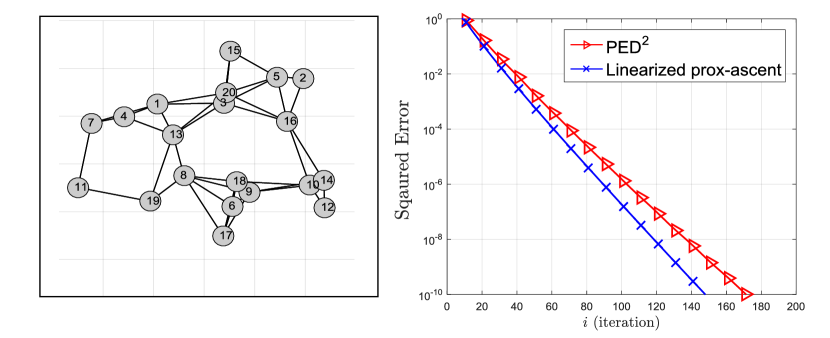
Figure 1: The network topology used in the simulation and squared error $\|{\scriptstyle{\mathcal{W}}}_{i}-{\scriptstyle{\mathcal{W}}}^{\star}\|^{2}$ evolution of the proposed PED² (15) and the centralized algorithm (24) with $\mu_{w}=0.03$ and $\mu_{y}=2$.

VII Conclusion

We studied the sharing problem (1), where agents are coupled through a convex possibly non-smooth composite function. To solve (1) in a decentralized manner, we reformulated it into an equivalent saddle-point problem. We then proposed a proximal decentralized algorithm and established its linear convergence. To our knowledge, this is the first decentralized linear convergence result for the multi-agent sharing problem (1) with a general non-smooth coupling function.

Appendix A Proof of Theorem 1

The following lemma establishes a useful equality, whose proof is omitted due to space limitations.

Lemma 3.

(Equality) Assume that the step-sizes $\mu_{w}$ and $\mu_{y}$ are strictly positive. The iterates of (12) satisfy:

$$\|\widetilde{\scriptstyle{\mathcal{W}}}_{i}\|^{2}_{I-\mu_{y}\mu_{w}{\mathcal{B}}_{d}^{\mathsf{T}}{\mathcal{B}}_{d}}+c_{y}\|\widetilde{\scriptstyle{\mathcal{Z}}}_{i}\|_{I-{\mathcal{L}}^{2}}^{2}+c_{y}\|\widetilde{\scriptstyle{\mathcal{X}}}_{i}\|^{2}$$

$$= \|\widetilde{\scriptstyle{\mathcal{W}}}_{i-1}-\mu_{w}({\nabla}{\mathcal{J}}({\scriptstyle{\mathcal{W}}}_{i-1})-{\nabla}{\mathcal{J}}({\scriptstyle{\mathcal{W}}}^{o}))\|^{2}$$

$$+c_{y}\|\widetilde{\scriptstyle{\mathcal{Y}}}_{i-1}\|_{I-\mu_{w}\mu_{y}{\mathcal{B}}_{d}{\mathcal{B}}_{d}^{\mathsf{T}}}^{2}+c_{y}\|\widetilde{\scriptstyle{\mathcal{X}}}_{i-1}\|_{I-{\mathcal{L}}^{2}}^{2},$$ (25)

where $c_{y}=\mu_{w}/\mu_{y}$. ∎

It can be verified that

$$\|\widetilde{\scriptstyle{\mathcal{W}}}_{i-1}-\mu_{w}({\nabla}{\mathcal{J}}({\scriptstyle{\mathcal{W}}}_{i-1})-{\nabla}{\mathcal{J}}({\scriptstyle{\mathcal{W}}}^{o}))\|^{2}$$

$$\leq \big{(}1-\tfrac{2\mu_{w}\delta\nu}{\delta+\nu}\big{)}\|\widetilde{\scriptstyle{\mathcal{W}}}_{i-1}\|^{2}$$

$$\leq \left({1-{2\mu_{w}\delta\nu\over\delta+\nu}\over 1-\mu_{y}\mu_{w}\sigma_{\max}^{2}({\mathcal{B}}_{d})}\right)\|\widetilde{\scriptstyle{\mathcal{W}}}_{i-1}\|_{I-\mu_{w}\mu_{y}{\mathcal{B}}_{d}^{\mathsf{T}}{\mathcal{B}}_{d}}^{2}.$$ (26)

where the first inequality holds under Assumption 1 for $\mu_{w}\leq{2\over\delta+\nu}$ – see [30]. The second inequality holds if $I-\mu_{y}\mu_{w}{\mathcal{B}}_{d}^{\mathsf{T}}{\mathcal{B}}_{d}$ is positive definite. Let

$$\gamma_{1}\;\stackrel{{\scriptstyle\Delta}}{{=}}\;{1-{2\mu_{w}\delta\nu\over\delta+\nu}\over 1-\mu_{y}\mu_{w}\sigma_{\max}^{2}({\mathcal{B}}_{d})}.$$ (27)

Then, we have $\gamma_{1}<1$ if $\mu_{y}<{2\delta\nu\over(\delta+\nu)\sigma_{\max}^{2}({\mathcal{B}}_{d})}$. Since the proximal mapping is nonexpansive, it holds from (20d) that:

$$\|\widetilde{\scriptstyle{\mathcal{Y}}}_{i}\|^{2} =\|{\mathrm{p}rox}_{\mu_{y}{\mathcal{G}}^{*}}(\bar{{\mathcal{A}}}{\scriptstyle{\scalebox{0.85}{\mbox{$\displaystyle\mathcal{Z}$}}}}_{i})-{\mathrm{p}rox}_{\mu_{y}{\mathcal{G}}^{*}}(\bar{{\mathcal{A}}}{\scriptstyle{\scalebox{0.85}{\mbox{$\displaystyle\mathcal{Z}$}}}}^{o})\|^{2}$$

$$\leq\|\bar{{\mathcal{A}}}\widetilde{\scriptstyle{\mathcal{Z}}}_{i}\|^{2}=\|\widetilde{\scriptstyle{\mathcal{Z}}}_{i}\|_{\bar{{\mathcal{A}}}^{2}}^{2}\leq\|\widetilde{\scriptstyle{\mathcal{Z}}}_{i}\|_{I-{\mathcal{L}}^{2}}^{2},$$ (28)

where the last inequality holds due to Assumption 2. Since each $B_{k}$ has full row rank, it holds that

$$0<\lambda_{\min}({\mathcal{B}}_{d}{\mathcal{B}}_{d}^{\mathsf{T}})I\leq{\mathcal{B}}_{d}{\mathcal{B}}_{d}^{\mathsf{T}}$$ (29)

where $\lambda_{\min}(\cdot)$ denotes the smallest eigenvalue of its argument. Therefore,

$$\|\widetilde{\scriptstyle{\mathcal{Y}}}_{i-1}\|_{I-\mu_{w}\mu_{y}{\mathcal{B}}_{d}{\mathcal{B}}_{d}^{\mathsf{T}}}^{2}\leq\big{(}1-\mu_{w}\mu_{y}\lambda_{\min}({\mathcal{B}}_{d}{\mathcal{B}}_{d}^{\mathsf{T}})\big{)}\|\widetilde{\scriptstyle{\mathcal{Y}}}_{i-1}\|^{2}.$$ (30)

Finally, since ${\scriptstyle{\scalebox{0.7}{\mbox{$\displaystyle\mathcal{X}$}}}}_{-1}=0$ and ${{\scriptstyle{\scalebox{0.7}{\mbox{$\displaystyle\mathcal{X}$}}}}}^{o}$ are in the range space of ${\mathcal{L}}$, the error quantity $\widetilde{\scriptstyle{\mathcal{X}}}_{i-1}$ always belongs to the range space of ${\mathcal{L}}$. This implies that $\|\widetilde{\scriptstyle{\mathcal{X}}}_{i-1}\|_{{\mathcal{L}}^{2}}^{2}\geq\underline{\sigma}^{2}({\mathcal{L}})\|\widetilde{\scriptstyle{\mathcal{X}}}_{i-1}\|^{2}$ where $\underline{\sigma}^{2}({\mathcal{L}})$ denotes the minimum non-zero singular value of ${\mathcal{L}}$ – see [29, Lemma 1]. Therefore,

$$\|\widetilde{\scriptstyle{\mathcal{X}}}_{i-1}\|_{I-{\mathcal{L}}^{2}}^{2}\leq(1-\underline{\sigma}^{2}({\mathcal{L}}))\|\widetilde{\scriptstyle{\mathcal{X}}}_{i-1}\|^{2}$$ (31)

Substituting the bounds (26), (28), (30), and (31) into (25) gives:

$$\|\widetilde{\scriptstyle{\mathcal{W}}}_{i}\|^{2}_{I-\mu_{y}\mu_{w}{\mathcal{B}}_{d}^{\mathsf{T}}{\mathcal{B}}_{d}}+c_{y}\|\widetilde{\scriptstyle{\mathcal{Y}}}_{i}\|^{2}+c_{y}\|\widetilde{\scriptstyle{\mathcal{X}}}_{i}\|^{2}$$

$$\leq\gamma_{1}\|\widetilde{\scriptstyle{\mathcal{W}}}_{i-1}\|_{I-\mu_{y}\mu_{w}{\mathcal{B}}_{d}^{\mathsf{T}}{\mathcal{B}}_{d}}^{2}+\gamma_{2}c_{y}\|\widetilde{\scriptstyle{\mathcal{Y}}}_{i-1}\|^{2}+\gamma_{3}c_{y}\|\widetilde{\scriptstyle{\mathcal{X}}}_{i-1}\|^{2},$$ (32)

where $\gamma_{2}\;\stackrel{{\scriptstyle\Delta}}{{=}}\;1-\mu_{w}\mu_{y}\lambda_{\min}({\mathcal{B}}_{d}{\mathcal{B}}_{d}^{\mathsf{T}})$ and $\gamma_{3}\;\stackrel{{\scriptstyle\Delta}}{{=}}\;1-\underline{\sigma}^{2}({\mathcal{L}})$. Under the step-size conditions given in (21), it holds that $I-\mu_{y}\mu_{w}{\mathcal{B}}_{d}^{\mathsf{T}}{\mathcal{B}}_{d}>0$ and $\gamma=\max\{\gamma_{1},\gamma_{2},\gamma_{3}\}<1$. Moreover, we have that $(1-\mu_{y}\mu_{w}\sigma_{\max}^{2}({\mathcal{B}}_{d}))\|\widetilde{\scriptstyle{\mathcal{W}}}_{i}\|^{2}\leq\|\widetilde{\scriptstyle{\mathcal{W}}}_{i}\|^{2}_{I-\mu_{y}\mu_{w}{\mathcal{B}}_{d}^{\mathsf{T}}{\mathcal{B}}_{d}}$. Let

$$C_{o}={\|\widetilde{\scriptstyle{\mathcal{W}}}_{-1}\|_{I-\mu_{y}\mu_{w}{\mathcal{B}}_{d}^{\mathsf{T}}{\mathcal{B}}_{d}}^{2}+c_{y}\|\widetilde{\scriptstyle{\mathcal{Y}}}_{-1}\|^{2}+c_{y}\|\widetilde{\scriptstyle{\mathcal{X}}}_{-1}\|^{2}\over 1-\mu_{y}\mu_{w}\sigma_{\max}^{2}({\mathcal{B}}_{d})}.$$ (33)

Iterating inequality (32) yields the result.

References

- [1] S. Boyd, N. Parikh, E. Chu, B. Peleato, and J. Eckstein, “Distributed optimization and statistical learning via alternating direction method of multipliers,” Found. Trends Mach. Lear., vol. 3, no. 1, pp. 1–122, 2011.
- [2] S. Sundhar Ram, A. Nedić, and V. V. Veeravalli, “A new class of distributed optimization algorithms: Application to regression of distributed data,” Optimization Methods and Software, vol. 27, no. 1, pp. 71–88, 2012.
- [3] J. Chen, Z. J. Towfic, and A. H. Sayed, “Dictionary learning over distributed models,” IEEE Trans. Signal Process., vol. 63, no. 4, pp. 1001–1016, 2015.
- [4] D. Hallac, J. Leskovec, and S. Boyd, “Network LASSO: Clustering and optimization in large graphs,” in ACM SIGKDD International Conference on Knowledge Discovery and Data Mining, 2015, pp. 387–396.
- [5] T.-H. Chang, A. Nedić, and A. Scaglione, “Distributed constrained optimization by consensus-based primal-dual perturbation method,” IEEE Trans. Autom. Control, vol. 59, no. 6, pp. 1524–1538, 2014.
- [6] D. P. Palomar and M. Chiang, “A tutorial on decomposition methods for network utility maximization,” IEEE Journal on Selected Areas in Communications, vol. 24, no. 8, pp. 1439–1451, 2006.
- [7] P. Chen, J. Huang, and X. Zhang, “A primal-dual fixed point algorithm for convex separable minimization with applications to image restoration,” Inverse Problems, vol. 29, no. 2, p. 025011, Jan. 2013.
- [8] N. Dhingra, S. Khong, and M. Jovanovic, “The proximal augmented Lagrangian method for nonsmooth composite optimization,” IEEE Trans. Autom. Control, vol. 64, no. 7, pp. 2861–2868, 2019.
- [9] W. Deng and W. Yin, “On the global and linear convergence of the generalized alternating direction method of multipliers,” Journal of Scientific Computing, vol. 66, no. 3, pp. 889–916, 2016.
- [10] L. Walras, Elements Deconomie Politique Pure, ou, Theorie de la Richesse Sociale. F. Rouge, 1896.
- [11] Y. Ho, L. Servi, and R. Suri, “A class of center-free resource allocation algorithms,” in IFAC Proceedings, vol. 13, Toulouse, France, 1980, pp. 475–482.
- [12] I. Necoara, “Random coordinate descent algorithms for multi-agent convex optimization over networks,” IEEE Trans. Autom. Control, vol. 58, no. 8, pp. 2001–2012, 2013.
- [13] T. T. Doan and A. Olshevsky, “Distributed resource allocation on dynamic networks in quadratic time,” Systems & Control Letters, vol. 99, pp. 57–63, 2017.
- [14] A. Nedić, A. Olshevsky, and W. Shi, “Improved convergence rates for distributed resource allocation,” in IEEE Conference on Decision and Control (CDC), Miami Beach, FL, USA, 2018, pp. 172–177.
- [15] J. Xu, S. Zhu, Y. C. Soh, and L. Xie, “A dual splitting approach for distributed resource allocation with regularization,” IEEE Transactions on Control of Network Systems, vol. 6, no. 1, pp. 403–414, 2018.
- [16] T. Yang, D. Wu, H. Fang, W. Ren, H. Wang, Y. Hong, and K. H. Johansson, “Distributed energy resources coordination over time-varying directed communication networks,” IEEE Transactions on Control of Network Systems, vol. 6, no. 3, pp. 1124–1134, 2019.
- [17] T.-H. Chang, M. Hong, and X. Wang, “Multi-agent distributed optimization via inexact consensus ADMM,” IEEE Trans. Signal Process., vol. 63, no. 2, pp. 482–497, Jan. 2015.
- [18] S. A. Alghunaim, K. Yuan, and A. H. Sayed, “A proximal diffusion strategy for multi-agent optimization with sparse affine constraints,” IEEE Trans. Autom. Control, 2020, early access (to appear).
- [19] B. Ying, K. Yuan, and A. H. Sayed, “Supervised learning under distributed features,” IEEE Trans. Signal Process., vol. 67, no. 4, pp. 977–992, 2019.
- [20] L. He, A. Bian, and M. Jaggi, “COLA: Decentralized linear learning,” in Advances in Neural Information Processing Systems (NeurIPS), 2018, pp. 4536–4546.
- [21] J. Tsitsiklis, D. Bertsekas, and M. Athans, “Distributed asynchronous deterministic and stochastic gradient optimization algorithms,” IEEE Trans. Autom. Control, vol. 31, no. 9, pp. 803–812, 1986.
- [22] A. Nedic and A. Ozdaglar, “Distributed subgradient methods for multi-agent optimization,” IEEE Trans. Autom. Control, vol. 54, pp. 48–61, 2009.
- [23] A. H. Sayed, “Adaptation, learning, and optimization over neworks,” Foundations and Trends in Machine Learning, vol. 7, pp. 311–801, 2014.
- [24] Y. Sun, A. Daneshmand, and G. Scutari, “Convergence rate of distributed optimization algorithms based on gradient tracking,” arXiv preprint:1905.02637, May 2019.
- [25] S. A. Alghunaim, K. Yuan, and A. H. Sayed, “A linearly convergent proximal gradient algorithm for decentralized optimization,” in Advances in Neural Information Processing Systems, 2019, pp. 2844–2854.
- [26] S. A. Alghunaim, E. K. Ryu, K. Yuan, and A. H. Sayed, “Decentralized proximal gradient algorithms with linear convergence rates,” submitted for publication, Sept. 2019, available on arXiv:1909.06479.
- [27] R. T. Rockafellar, Convex Analysis. Citeseer, 1970.
- [28] H. H. Bauschke and P. L. Combettes, Convex Analysis and Monotone Operator Theory in Hilbert Spaces. Springer, 2011, vol. 408.
- [29] S. A. Alghunaim and A. H. Sayed, “Linear convergence of primal-dual gradient methods and their performance in distributed optimization,” Automatica, vol. 117, pp. 1–8, July 2020.
- [30] Y. Nesterov, Introductory Lectures on Convex Optimization: A Basic Course. Springer, 2013, vol. 87.