Transport coefficients of multi-component mixtures of noble gases based on ab initio potentials. Viscosity and thermal conductivity.

Abstract

The viscosity and thermal conductivity of binary, ternary and quaternary mixtures of helium, neon, argon, and krypton at low density are computed for wide ranges of temperature and molar fractions, applying the Chapman-Enskog method. Ab initio interatomic potentials are employed in order to calculate the omega-integrals. The relative numerical errors of the viscosity and thermal conductivity do not exceed $10^{-6}$ and 10^-5, respectively. The relative uncertainty related to the interatomic potential is about 0.1%. A comparison of the present data with results reported in other papers available in the literature shows a significant improvement of accuracy of the transport coefficients considered here.

Key words: multi-component gaseous mixture, viscosity, thermal conductivity, ab initio potential.

I Introduction

The technique to calculate viscosity and thermal conductivity for binary gaseous mixtures is well elaborated and published in numerous papers, see e.g., Refs. Tip02 ; Tip03 ; Tom04 ; Tom05 ; Son49 ; Sha110 ; Sha118 ; Sha126 . The approach of these works is based on the Chapman-Enskog method Cha04 ; Fer02 applied to a system of the kinetic Boltzmann equations. This method and experimental data on the transport coefficients were analyzed by Kestin et al. Kes01 in order to derive empirical expressions of viscosity and thermal conductivity for all kinds of mixtures of the noble gases.

In practice, one deals with ternary and quaternary mixtures of noble gases as often as with binary ones, see e.g. Refs. Loy36 ; Ben03 ; Sza06 ; Yak02 , so that reliable data on the transport coefficients for ternary, quaternary, etc. mixtures are also of practical and scientific interest. These coefficients are included in the Navier-Stokes equations describing fluid flows in continuous medium regime. Moreover, the viscosity coefficient is important in rarefied gas dynamics Sha02B in order to determine the equivalent-free-path used to calculate the rarefaction parameter Fre04 ; Sha56 ; Sha100 ; HoM03 ; Val10 ; Gos03 velocity slip Sha54 ; Sha84 , and temperature jump Sha55 coefficients. The rarefaction parameter, velocity slip, and temperature jump are widely used in modelling of micro and nano flows of gases.

The general theory of the transport coefficients described by Ferziger & Kaper Fer02 is valid for an arbitrary number of gaseous species. The final expressions of the coefficients are cumbersome and given in term of solution of a large system of algebraic equations. The matrix elements of the system and free terms are linear combinations of multi-fold integrals which depend on the interatomic potential. To overcome the great numerical difficulties, some approximate formulas of the transport coefficients were proposed, see e.g. the papers Bro05 ; Sin02 ; Avs01 , which contain some fitting parameters, usually, extracted from experimental data.

Nowadays, ab initio potentials for all pairs that can be composed from helium, neon, argon, and krypton are available in the open literature, see e.g. Refs. Azi03 ; Cyb01 ; Hal01 ; Cac01 ; Hel03 ; Pat02 ; Prz01 ; Cen01 ; Jag02 ; Jag03 ; Jag04 . This information allows us to obtain the transport coefficient of any multi-component mixture of these noble gases.

Some binary mixture were considered in previously published papers, namely, the helium-neon mixture was considered in Ref. Sha118 , the transport coefficients of helium-argon and neon-argon mixtures were reported in Ref. Sha126 , and the same coefficients of helium-krypton mixture were calculated in Ref. Jag04 . However, the transport coefficient of ternary and quaternary mixtures of the noble gases have not been calculated yet on the basis of ab initio potentials. Accurate results for some binary mixtures of the noble gases are also absent in the literature.

In the present paper, numerical results on viscosity and thermal conductivity of binary, ternary and quaternary mixtures of helium, neon, argon and krypton in the temperature range from 50 K to 5000 K based on ab initio potentials are reported. The quantum approach to the interatomic interactions is employed for all kinds of collisions. The relative numerical error of the viscosity and thermal conductivity is less then $10^{-6}$ and $10^{-5}$, respectively. The estimated relative uncertainty due to the interatomic potential does not exceed 0.1% and in some cases can be even smaller.

II Statement of the problem.

Here, we consider a mixture of $K$ monatomic gases at a temperature $T$ and pressure $p$. The number density of each species is denoted as $n_{i}$ ($1\leq i\leq K$). The chemical composition of the mixture can be characterized by the mole fraction defined as

$$x_{i}=n_{i}/n,\quad n=\sum_{i=1}^{K}n_{i}.$$ (1)

The mixture pressure is assumed to be so low that the state equation corresponds to ideal gas, i.e. $p=nk_{\mbox{\tiny B}}T$, where $k_{\mbox{\tiny B}}$ is the Boltzmann constant.

We are going to calculate the dynamic viscosity $\mu$ and thermal conductivity $\kappa$ of binary, ternary and quaternary mixtures of helium, neon, argon and krypton as a function of the temperature $T$ and chemical composition $x_{i}$. The calculations are based on ab initio potentials available in the open literature.

The viscosity $\mu$ is well defined in fluid mechanics, see e.g. Ref. Lan05 , while the thermal conductivity requires some clarifications. According to the papers Muc01 ; Fer02 , there are two kinds of thermal conductivity coefficients of mixture: partial coefficient $\kappa^{\prime}$ and steady state coefficient $\kappa$. The former one $\kappa^{\prime}$ characterizes a heat transfer through a mixture with an uniform chemical composition. In this case, each species of the mixture moves due to the thermal diffusion phenomenon, while the whole mixture is at rest. The latter coefficient $\kappa$ corresponds to situation when the thermal diffusion is compensated by diffusion and a time-independent mole fraction distribution is established. Under this condition, all species of the mixture are at rest. The coefficients are coupled to each other by, see Sec 6.3 from the book Fer02 ,

$$\kappa^{\prime}=\kappa+nk_{\mbox{\tiny B}}\sum_{i=1}^{K}k_{Ti}D_{Ti},$$ (2)

where $k_{Ti}$ is the thermal diffusion ratio of species $i$ and $D_{Ti}$ is the thermal diffusion coefficient related as

$$\sum_{j=1}^{K}D_{ij}k_{Ti}=D_{Ti},$$ (3)

with $D_{ij}$ being the multi-component diffusion coefficient. Like our previous papers, we are going to calculate the steady state thermal coefficient $\kappa$. Once the coefficients $D_{ij}$ and $D_{Ti}$ are known, the partial coefficient $\kappa^{\prime}$ can be calculated too.

III Method of calculation.

III.1 Expressions of transport coefficients

The expressions of the transport coefficients for multi-component mixture are derived by the Chapman-Enskog method applied to the kinetic Boltzmann equation in the book by Ferziger & Kaper Fer02 . In case of binary mixture, this method is well described in the book Cha04 and the papers Tip02 ; Tip03 ; Tom04 ; Tom05 . The expression for viscosity $\mu$ of multi-component obtained in Ref. Fer02 in term of bracket integrals are used here with slightly different notations. Each bracket integral contains information about only two gaseous species so that the expressions of these integrals obtained in Refs. Tip02 ; Tip03 ; Tom04 ; Tom05 can be used here for multi-component mixture. Since the book Fer02 does not provide the explicit expression of $\kappa$, its derivations for binary mixture Tip03 is generalized for multi-component mixture in Appendix to the present paper.

Following the previously published derivations Fer02 ; Tip02 ; Tip03 ; Tom04 ; Tom05 and those given in Appendix, the viscosity $\mu$ and thermal conductivity $\kappa$ are calculated as

$$\mu=\frac{5}{2}k_{\mbox{\tiny B}}T\sum_{i=1}^{K}x_{i}b^{(1)}_{i},$$ (4)

$$\kappa=\frac{75}{8}k_{\mbox{\tiny B}}^{2}T\sum_{i=1}^{K}\frac{x_{i}}{\sqrt{m_{i}}}a^{(1)}_{i},$$ (5)

respectively. The coefficients $a_{i}^{(1)}$ and $b_{i}^{(1)}$ are calculated from the corresponding systems of algebraic equations

$$\sum_{j=1}^{K}\sum_{q=1}^{N}A_{ij}^{(pq)}a_{j}^{(q)}=\frac{x_{i}\delta_{p1}}{\sqrt{m_{i}}},$$ (6)

$$\sum_{j=1}^{K}\sum_{q=1}^{N}B_{ij}^{(pq)}b^{(q)}_{j}=x_{i}\delta_{p1},\quad$$ (7)

where $1\leq i\leq K$, $1\leq p\leq N$, $\delta_{pq}$ is the Kronecker delta, and $N$ is the order of approximation. The values of $\mu$ and $\kappa$ converge to their exact values in the limit $N\to\infty$. The matrices $A_{ij}^{(pq)}$, $B_{ij}^{(pq)}$ are expressed in terms of the bracket integrals as

$$A_{ii}^{(pq)}=x_{i}^{2}\left[S_{3/2,i}^{(p)}\boldsymbol{\mathscr{C}}_{i},S_{3/2,i}^{(q)}\boldsymbol{\mathscr{C}}_{i}\right]_{i}$$

$$\hskip 28.45274pt+\sum_{\begin{subarray}{c}j=1\\ j\neq i\end{subarray}}^{N}x_{i}x_{j}\left[S_{3/2,i}^{(p)}\boldsymbol{\mathscr{C}}_{i},S_{3/2,i}^{(q)}\boldsymbol{\mathscr{C}}_{i}\right]_{ij},$$ (8)

$$A_{ij}^{(pq)}=x_{i}x_{j}\left[S_{3/2,i}^{(p)}\boldsymbol{\mathscr{C}}_{i},S_{3/2,j}^{(q)}\boldsymbol{\mathscr{C}}_{j}\right]_{ij},\quad i\neq j,$$ (9)

$$B_{ii}^{(pq)}=x_{i}^{2}\left[S_{5/2,i}^{(p-1)}\boldsymbol{\mathsf{C}}_{i},S_{5/2,i}^{(q-1)}\boldsymbol{\mathsf{C}}_{i}\right]_{i}$$

$$\hskip 28.45274pt+\sum_{\begin{subarray}{c}j=1\\ j\neq i\end{subarray}}^{N}x_{i}x_{j}\left[S_{5/2,i}^{(p-1)}\boldsymbol{\mathsf{C}}_{i},S_{5/2,i}^{(q-1)}\boldsymbol{\mathsf{C}}_{i}\right]_{ij}$$ (10)

$$B_{ij}^{(pq)}=x_{i}x_{j}\left[S_{5/2,i}^{(p-1)}\boldsymbol{\mathsf{C}}_{i},S_{5/2,j}^{(q-1)}\boldsymbol{\mathsf{C}}_{j}\right]_{ij},\quad i\neq j$$ (11)

where $S_{\nu,i}^{(p)}$ are the Sonine polynomials with the argument $\mathscr{C}_{i}^{2}$, i.e.

$$S_{\nu,i}^{(p)}=\sum_{n=0}^{p}\frac{\Gamma(\nu+p+1)}{(p-n)!n!\Gamma(\nu+n)}\left(-\mathscr{C}^{2}_{i}\right)^{n}.$$ (12)

The tensor $\boldsymbol{\mathsf{C}}_{i}$ is defined as

$$\boldsymbol{\mathsf{C}}_{i}=\boldsymbol{\mathscr{C}}_{i}\boldsymbol{\mathscr{C}}_{i}-\frac{1}{3}\mathscr{C}^{2}_{i}\boldsymbol{\mathsf{I}},$$ (13)

with $\boldsymbol{\mathsf{I}}$ being the identity tensor. The dimensional molecular velocity $\boldsymbol{\mathscr{C}}_{i}$ is defined for each species as

$$\boldsymbol{\mathscr{C}}_{i}=\sqrt{\frac{m_{i}}{2k_{\mbox{\tiny B}}T}}{\boldsymbol{C}}_{i},\quad{\boldsymbol{C}}_{i}={\boldsymbol{c}}_{i}-{\boldsymbol{u}},$$ (14)

where $m_{i}$ is the atomic mass of species $i$, ${\boldsymbol{c}}_{i}$ is its molecular velocity, and ${\boldsymbol{u}}$ is the hydrodynamic velocity of the mixture. Some of the bracket integrals are given in the book Fer02 . The general expressions of bracket integrals for arbitrary orders $p$ and obtained in the papers Tom04 ; Tom05 for binary mixtures can be used here. The first and second brackets in Eq.(8) are given by Eqs.(119) and (117) from Ref. Tom04 , respectively. The brackets in Eq.(9) are given by Eq.(115) from Ref. Tom05 . The first and second brackets in Eq.(10) are given by Eqs.(113) and (111) from Ref. Tom05 , respectively. The brackets in Eq.(11) are given by Eq.(109) from Ref. Tom05 . To generalize the corresponding expressions given in the papers Tom05 ; Tom04 to a multi-component mixture, the subscripts “1” and ”2” are replaced by “i” and “j”, respectively. In case of $i>j$, the symmetry relations

$$A^{(pq)}_{ij}=A_{ji}^{(qp)},\quad B^{(pq)}_{ij}=B_{ji}^{(qp)}$$ (15)

are employed.

III.2 Transport cross sections

The matrices $A^{(pq)}_{ij}$, $B^{(pq)}_{ij}$ are given in terms of the $\Omega$-integrals defined as

$$\Omega_{ij}^{(n,r)}=\sqrt{\frac{k_{\mbox{\tiny B}}T}{8\pi m_{ij}}}\int_{0}^{\infty}Q^{(n)}_{ij}\;\varepsilon^{r+1}e^{-\varepsilon}\,\mbox{d}\varepsilon,$$ (16)

where $\varepsilon$ is the dimensionless energy of interacting particles

$$\varepsilon=\frac{E}{k_{\mbox{\tiny B}}T},\quad E=\frac{1}{2}m_{ij}|{\boldsymbol{c}}_{i}-{\boldsymbol{c}}_{j}|^{2},\quad i,j=1,2,$$ (17)

$m_{ij}={m_{i}m_{j}}/(m_{i}+m_{j})$ is the reduced mass of interaction particles. The transport cross sections $Q^{(n)}_{ij}$ for two different particles are calculated in terms of scattering phase shifts $\delta_{l}$ Mee01

$$Q^{(n)}_{ij}=\frac{2\pi\hbar^{2}}{m_{ij}E}\sum_{l=0}^{\infty}\sum_{j=0}^{\lfloor(n-1)/2\rfloor}C_{lj}^{(n)}\sin^{2}\left(\delta_{l}-\delta_{l+n-2j}\right),$$ (18)

where $\hbar$ is the reduced Planck constant. The coefficients $C^{(n)}_{lj}$ are given by Eq.(12) in the previous paper Sha118 . For indistinguishable bosons with spin equal to zero, Eq.(18) should be modified by retaining only even indices $l$ and multiplying the expression (18) by the factor 2.

The numerical scheme to calculate the phase shifts $\delta_{l}$ is given in details in our previous works Sha118 ; Sha126 so that here, only some its improvements will be described. As is known, the the Schrödinger equation is solved for relatively small values of the index $l$, i.e. $l\leq l_{q}$. Then, the semi-classical WKB method Joa01 ; Shi07 is used in case of large values of $l$, i.e. $l>l_{q}$. The value of $l_{q}$ for the transition from the quantum approach to the semi-classical one depends on the interaction energy $E$ and species of interacting gases. In the present work, the spherical Bessel and Neumann functions used in the quantum approach have been calculated with the quadruple precision, which allowed us to increase significantly the transition value $l_{q}$. Now, it is given by the expression

$$l_{q}=\lfloor A\cdot E^{1/4}\rfloor,$$ (19)

where the energy $E$ is measured in kelvin. However, its value must be always smaller than $l_{q,max}$. The values of the parameter $A$ and that of the limit $l_{q,max}$ are given in Table 1.

Table 1: Parameters in Eqs.(19)-(20), references about potentials used in the present work, and relative uncertainties $u_{ij}$ of viscosity and thermal conductivity due to potential.

pair	Parameters
	$A$(K-1/4)	$l_{q,max}$	$B$(K1/2)	$R_{0}$ (nm)	Refs.	$u_{ij}$
He-He	18	450	1.3	0.264099	Cen01	$10^{-5}$
Ne-Ne	30	600	2.0	0.276125	Hel03	$10^{-3}$
Ar-Ar	60	1200	3.0	0.335772	Pat02	$10^{-4}$
Kr-Kr	70	1600	3.5	0.358089	Jag03	$10^{-3}$
He-Ne	22	600	1.4	0.269879	Cac01	$10^{-3}$
He-Ar	22	600	2.0	0.311691	Cac01	$10^{-4}$
He-Kr	22	600	2.0	0.328702	Jag04	$10^{-3}$
Ne-Ar	40	900	2.3	0.312206	Cac01	$10^{-4}$
Ne-Kr	50	950	2.3	0.326543	Hal01	$10^{-3}$
Ar-Kr	70	1400	3.5	0.347762	Hal01	$10^{-3}$

The quadruple precision also allowed to increase the point $r_{m}$ where the phase shift is calculated. In the present work, it is given by

$$r_{m}=10^{3}\;R_{0}\frac{B}{\sqrt{E}},$$ (20)

where the energy $E$ is measured in kelvin and $R_{0}$ is the zero point of the interatomic potential, i.e., $V(R_{0})=0$. The values of $B$ and $R_{0}$ are given in Table 1. The value of $r_{m}$ does not exceed the limit $10^{3}R_{0}$. The integration step is given by

$$\Delta r=R_{0}\frac{C}{\sqrt[3]{E}},\quad C=10^{-3}\mbox{ K}^{1/3}.$$ (21)

The upper limit for $\Delta r$ is 10${}^{-3}R_{0}$.

The fundamental constants, such as the Bohr radius, atomic mass constant, and Hartree energy are taken from the CODATA-2014 recommended values Moh03 . The atomic masses $m_{\mbox{\tiny He}}=4.002602$, $m_{\mbox{\tiny Ne}}=20.1797$, $m_{\mbox{\tiny Ar}}=39.948$, and $m_{\mbox{\tiny Kr}}=83.798$ measured in the atomic mass constant are taken from Ref. Mei02 .

The transport cross sections $Q^{(n)}_{ij}(E)$ for the six kinds of collisions have been calculated once for many values of the energy $E$. These quantities are smooth functions of the energy $E$ in the range $E>100$ K, while they have unpredictable behaviours at the small energies. The cross sections $Q_{ii}^{(2)}$ ($i=1,2$) for collisions between the identical particles, namely, Ne-Ne, Ar-Ar,and Kr-Kr are depicted in Figure 1, which shows that all of them have many sharp peaks. The cross sections $Q_{12}^{(1)}$ for collisions between different particles, viz., He-Kr, Ne-Kr, and Ar-Kr plotted in Figure 2 also have many sharp peaks. Such behaviours of the transport cross sections represent a difficulty to calculate the $\Omega$-integrals (16) so that the energy nodes should be distributed non-uniformly. Here, we use a larger number of the nodes $E_{m}$ than that used previously Sha118 ; Sha126 , that is

$$E_{m}=2\,(1.00025^{m}-1),\quad 1\leq m\leq 48000.$$ (22)

Then, the $\Omega$-integrals (16) are calculated using these knots by the simple trapezoidal rule.

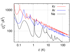
Figure 1: Transport cross section $Q_{ii}^{(2)}$ for Ne, Ar, and Kr vs. collision energy $E$.

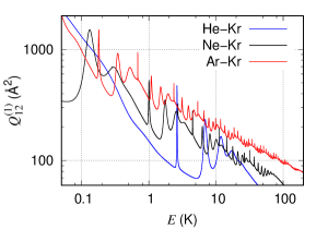
Figure 2: Transport cross section $Q_{12}^{(1)}$ for He-Kr, Ne-Kr, and Ar-Kr collisions vs. energy $E$.

IV Potentials

According to Ref. Sha126 , the phase shifts used to calculate the $\Omega$-integrals substituted into the matrices $A_{ij}^{(pq)}$ and $B_{ij}^{(pq)}$ are obtained from the Schrödinger equation containing the interatomic potential. Nowadays, there are many papers reporting ab initio potentials for homogeneous and heterogeneous dimers of four noble gases, see e.g. Refs. Cen01 ; Hel03 ; Pat02 ; Jag03 ; Cac01 ; Jag04 ; Hal01 ; Cyb01 ; Jag02 . The most reliable of then have been chosen for our calculations. The papers containing potentials used in the present work for main calculations are listed in the sixth column of Table 1.

V Uncertainty

There are two types of uncertainties in the present calculations. The first uncertainty is caused by numerical errors and the second uncertainty is related to interatomic potentials used in the calculations. In this section, these two uncertainties are analyzed and estimated separately.

There are several sources of numerical error in the transport coefficients such as: order of approximation $N$ in Eqs.(6) and (7), the value of the parameter $l_{q}$ for transition from the purely quantum approach to the semi-classical one, the point $r_{m}$ where the phase shift is calculated, the step of integration $\Delta r$ to solve the Schrödinger equation, the node distribution of the energy (22). The contribution of each error source has been estimated by varying the above mentioned parameters. The main calculations have been carried out for the order approximation $N=10$, the nodes given by (22), the parameters $l_{q}$, $r_{m}$, and $\Delta r$ given by Eq.(19), (20), and (21), respectively. Then, test calculations have been carried for $N=12$ with the nodes twice rarer than (22), decreasing $l_{q}$ and $r_{m}$ by the factor $0.8$, and increasing $\Delta r$ by the factor 1.5. An analysis of the test results showed that the main numerical contribution into the viscosity comes from the node distribution, which is equal to $\times 10^{-6}$. In case of the thermal conductivity, the main contribution in to the error budget is that because of the approximation order $N$ and equal to $10^{-5}$. In fact, the convergence with respect to the order $N$ for the viscosity is significantly higher than that for the thermal conductivity, especially, in case of the helium-krypton mixture Jag04 . All other source of the numerical error is orders of magnitude smaller. Thus, the total numerical error can be assumed to be $\times 10^{-6}$ for the viscosity and $10^{-5}$ for the thermal conductivity.

The potentials used in the present work have different degree of their uncertainty. For instance, the helium-helium potential causes the relative uncertainty of $10^{-5}$ in the transport coefficients Cen01 . At the moment, this is the most exact potential among all other available in the literature. The uncertainties of $\mu$ and $\kappa$ due to the neon-neon Bic01 and helium-neon Cac01 potentials estimated in Ref. Sha118 are equal to $10^{-3}$ over the temperature range considered here. The argon-argon Pat02 , helium-argon Cac01 , and neon-argon Cac01 potentials lead the relative uncertainties in the coefficients $\mu$ and $\kappa$ about $10^{-4}$ according to estimations in Ref. Sha126 . The uncertainties of the krypton-krypton and helium-krypton potentials estimated in Ref. Jag04 are equal to $10^{-3}$. The uncertainties of the neon-krypton and argon-krypton potentials proposed in Ref. Hal01 were not analyzed previously. However, the krypton-krypton potential elaborated in the same work Hal01 causes the uncertainty of $10^{-3}$ that can be used as the uncertainty estimation for the neon-krypton and argon-krypton potentials. All relative uncertainties are summarized in Table 1. As has been mentioned above, the potential is used to calculate the bracket integrals in Eqs.(8)-(11). Thus, each potential of interatomic interaction between species $i$ and $j$ contributes into the mixture transport coefficients proportionally to $x_{i}x_{j}$. Then, the total relative uncertainty can be estimated by

$$u=\sqrt{\sum_{i=1}^{K}\sum_{j=i}^{K}(x_{i}x_{j}u_{ij})^{2}},$$ (23)

where the uncertainties $u_{ij}$ are given in Table 1.

VI Results and discussions

VI.1 Remarks

In this section, the numerical results on the viscosity and thermal conductivity are presented and compared with some previously published works. Mainly, the present results will be compared with those reported by Kestin et al. Kes01 who analyzed an extensive database of the transport coefficients of all possible mixtures of noble gases. The authors of Ref. Kes01 obtained an empirical expressions of the coefficients and estimated their uncertainty by comparing with experimental data published before 1984. During the last decade, new experimental data of viscosity of some single gases were reported Ber15 ; Ber14 , but no significant progress has been done in measurements of the thermal conductivity and viscosity of gaseous mixture. Thus, the most of the numerical results obtained here will be compared with those reported by Kestin et al. Kes01 . When possible, a comparison with more accurate theoretical and experimental results is performed.

VI.2 Binary mixture

Some binary mixtures, namely, helium-neon, helium-argon, neon-argon were considered in our previous papers Sha118 ; Sha126 , where the viscosity and thermal conductivity were calculated with the relative numerical error less than $10^{-5}$ using the quantum approach. The authors of Ref. Jag04 reported numerical results on the transport coefficients for the helium-krypton mixture declaring the relative uncertainty about $10^{-3}$. Some binary mixtures were considered also in Ref. Son49 without an estimation of uncertainty. Below, numerical results on the binary mixtures not considered in our previous papers Sha118 ; Sha126 , namely, helium-krypton, neon-krypton, and argon-krypton are presented and compared with those reported in other works Kes01 ; Jag04 ; Son49 .

The numerical values of viscosity and thermal conductivity of the helium-krypton mixture including pure krypton ($x_{1}=0$) are reported in Table 2. Since the previous results on pure krypton Jag04 are based on the classical theory of interatomic collisions, it is worth to estimate the influence of the quantum effect on the transport coefficients. For this purpose, the transport cross sections $Q_{ij}^{(n)}$ in the $\Omega$-integrals (16) have been calculated applying the classical theory of interatomic collisions Sha110 for the nodes (22) of the energy $E$ with the relative numerical error less than $10^{-5}$. A comparison of the viscosity based on the quantum approach with that based on the classical one is shown in Figure 3. The deviation of the numerical results reported in Ref. Jag04 from those reported here is also plotted in Figure 3. Our results based on the classical approach are in agreement with those reported in Ref. Jag04 within $7\times 10^{-5}$ that is smaller than the accuracy declared by the authors of Ref. Jag04 . The plot depicted in Figure 3 shows that the influence of quantum effects reaches the order $5\times 10^{-4}$, i.e., it exceeds the numerical accuracy of the present work. The measured value of the krypton viscosity at the temperature $t=25^{\circ}$C reported by Berg & Burton Ber14 has the relative uncertainty of $3\times 10^{-4}$ and represents the most exact experimental results till now. The experimental uncertainty of this value plotted by cross in Figure 3 has the same order as the quantum effect. The deviation of the experimental value from that obtained in the present work is equal to 0.6$\times 10^{-4}$ that represents the smallest deviation among all theoretical results reported till now.

Jäger & Bich Jag04 proposed an ab initio potential for the pair helium-krypton considered by us as the most reliable one. Their numerical data on transport coefficients of the helium-krypton mixture are most exact among all data available in the open literature. They estimated the standard uncertainty of the viscosity to be 0.14% and that of thermal conductivity values to be 0.2%. Moreover, they computed all collision integrals for the Kr–Kr atom pair classically, while for Kr–He and He–He collisions, they employed the quantum-mechanical approach. Since we employed the same potentials for He-He, Kr-Kr, and He-Kr collisions as those used by Jäger & Bich Jag04 , the use of the classical approach is the main difference of their results from those reported here. Moreover, the present results have been obtained with higher numerical accuracy. The deviations of the results by Jäger & Bich Jag04 from the present ones are plotted in Figure 4. The deviations are within the uncertainty declared by the authors of Ref. Jag04 , but they are significantly larger than the numerical error of the present results. The maximum deviation for the viscosity is 0.04% at $T=$70 K and $x_{1}=0.2$. The greatest deviation of the thermal conductivity is about 0.14% at 1500 K and $x_{1}=0.2$. The larger deviation of the thermal conductivity is due to its slow convergence with respect to the approximation order $N$ in Eq.(6).

Table 2: Viscosity $\mu$ and thermal conductivity $\kappa$ vs. temperature $T$ and molar fraction $x_{1}$ of helium for He-Kr mixture.

	$\mu$($\mu$Pa$\cdot$s)				$\kappa$(mW/(m$\cdot$K))
$T$(K)	$x_{1}$=0.	0.25	0.5	0.75	$x_{1}$=0.	0.25	0.5	0.75
50.	4.95443	5.35481	5.88556	6.52356	1.84625	5.58588	11.4855	22.1846
100.	8.88984	9.56212	10.3950	11.2229	3.30924	9.75904	19.6828	36.9559
200.	17.3212	18.1263	18.9889	19.4045	6.44504	17.0077	33.0351	60.3896
300.	25.4260	26.1709	26.8203	26.5629	9.46314	23.3654	44.4019	80.1937
500.	39.4057	39.9862	40.2174	38.8167	14.6808	34.3240	64.0522	114.661
800.	56.4411	56.9211	56.8114	54.3162	21.0528	48.2624	89.4989	159.827
1000.	66.2527	66.7421	66.5366	63.5634	24.7243	56.5998	104.940	187.457
2000.	106.770	107.678	107.636	103.531	39.8743	92.7663	173.135	310.695
3000.	140.504	142.049	142.581	138.231	52.4740	124.330	233.649	421.098
5000.	199.071	202.081	204.185	200.402	74.3326	181.240	344.195	624.390

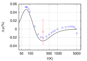
Figure 3: Deviation of viscosity $\Delta\mu(\%)=(\mu_{\mbox{\tiny O}}/\mu_{\mbox{\tiny P}}-1)\times 100$ of pure krypton based on other theoretical results (subscript “O”) from that calculated in the present work (subscript “P”): solid line - $\mu_{\mbox{\tiny O}}$ calculated by classical approach using the same potential as for $\mu_{\mbox{\tiny P}}$; circles - numerical values of $\mu_{\mbox{\tiny O}}$ reported in Ref. Jag04 ; cross - experimental results on $\mu_{\mbox{\tiny O}}$ reported in Ref. Ber14 .

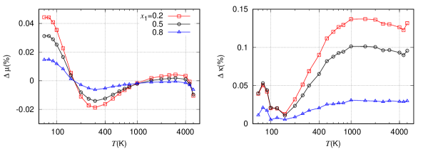
Figure 4: Deviation of viscosity (left) and thermal conductivity (right) of helium-krypton mixture reported by Jäger & and Bich Jag04 (subscript “J” ) from those calculated in the present work (subscript “P”), $\Delta C(\%)=(C_{\mbox{\tiny J}}/C_{\mbox{\tiny P}}-1)\times 100$, $C=\mu,\kappa$.

The transport coefficients $\mu$ and $\kappa$ for the neon-krypton mixture are reported in Table 3. In case of pure neon ($x_{1}=1$), the values of $\mu$ and $\kappa$ are exactly the same as those reported previously Bic02 ; Sha118 so that they are omitted in the present work. The most reliable data for this mixture are reported by Kestin et al. Kes01 with the uncertainty being 0.3% and 0.7% for the viscosity and thermal conductivity, respectively. A comparison of these data with the present results is performed in Figure 5. As one can notice, the deviations for both viscosity and thermal conductivity are within $\pm$1% in the temperature range 50 K$\leq T\leq$2000 K, while they jump up to -3 % at $T=3000$ K. Anyhow, the deviations exceed the uncertainties estimated in Ref. Kes01 and, especially, the total uncertainty of the present results.

Table 3: Viscosity $\mu$ and thermal conductivity $\kappa$ vs. temperature $T$ and molar fraction $x_{1}$ of neon for Ne-Kr mixture.

	$\mu$($\mu$Pa$\cdot$s)			$\kappa$(mW/(m$\cdot$K))
$T$(K)	$x_{1}$=0.25	0.5	0.75	0.25	0.5	0.75
50.	5.41149	6.00505	6.79213	3.07228	4.8161	7.48881
100.	9.93136	11.2223	12.7867	5.59787	8.84097	13.7915
200.	18.8837	20.6935	22.6437	10.2917	15.6929	23.8155
300.	27.0732	28.9004	30.7317	14.4565	21.4706	31.9872
500.	40.9781	42.6395	44.1657	21.516	31.1699	45.6578
800.	57.9745	59.5477	60.906	30.2509	43.2962	62.8854
1000.	67.8375	69.4528	70.825	35.3733	50.4856	73.1658
2000.	108.994	111.275	113.233	57.0164	81.2616	117.465
3000.	143.551	146.715	149.505	75.3856	107.652	155.616
5000.	203.834	208.848	213.412	107.669	154.310	223.176

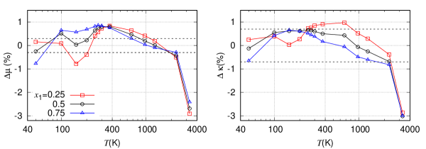
Figure 5: Deviation of viscosity (left) and thermal conductivity (right) of neon-krypton mixture reported by Kestin et al. Kes01 (subscript “K”) from those calculated in the present work (subscript “P”), $\Delta C(\%)=(C_{\mbox{\tiny K}}/C_{\mbox{\tiny P}}-1)\times 100$, $C=\mu,\kappa$, dashed lines - uncertainty declared in Ref. Kes01 .

The numerical data on the coefficients $\mu$ and $\kappa$ for the argon-krypton mixture are given in Table 4. The values of $\mu$ and $\kappa$ for pure argon are the same as those reported in the previous work Sha126 and not presented here. The paper by Song et al. Son49 also reported the transport coefficients for the argon-krypton mixture, obtained by the Chapman-Enskog method with the first order approximation, i.e., $N=1$ in Eqs.(6) and (7). They did not estimated the uncertainty of their results. Kestin et al. Kes01 provided their results on the argon-krypton mixture with the relative uncertainties being 0.4% and 0.5% for the viscosity and thermal conductivity, respectively. Figures 6 presents the comparison between the previously reported data Kes01 ; Son49 and those calculated here. The deviation of viscosity reported in Ref. Kes01 varies from -3% to 1% that is out of the predicted uncertainty over a wide range of the temperature. The data on viscosity provided in Ref. Son49 are closer to our results and deviate from them in the range from -1% to 2%. The behavior of the thermal conductivity deviation is very similar to that of the viscosity.

Table 4: Viscosity $\mu$ and thermal conductivity $\kappa$ vs. temperature $T$ and molar fraction $x_{1}$ of argon for Ar-Kr mixture

	$\mu$($\mu$Pa$\cdot$s)			$\kappa$(mW/(m$\cdot$K))
$T$(K)	$x_{1}$=0.25	0.5	0.75	0.25	0.5	0.75
50.	4.84845	4.71323	4.54053	2.12785	2.4679	2.8782
100.	8.78483	8.63446	8.42282	3.87782	4.55498	5.36563
200.	17.141	16.8652	16.4594	7.51387	8.81708	10.4149
300.	25.0243	24.4701	23.7146	10.9148	12.7115	14.9402
500.	38.4827	37.3122	35.8266	16.7315	19.3028	22.5157
800.	54.8465	52.897	50.5031	23.8417	27.3529	31.7413
1000.	64.2876	61.9068	59.0078	27.9568	32.0245	37.1008
2000.	103.412	99.3825	94.5187	45.053	51.5177	59.5207
3000.	136.088	130.78	124.362	59.3561	67.8875	78.3863
5000.	192.921	185.486	176.444	84.2641	96.4559	111.339

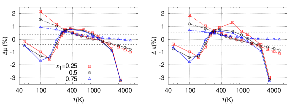
Figure 6: Deviation of viscosity (left) and thermal conductivity (right) of argon-krypton mixture reported in other papers (subscript “O”) from those calculated in the present work (subscript “P”), $\Delta C(\%)=(C_{\mbox{\tiny O}}/C_{\mbox{\tiny P}}-1)\times 100$, $C=\mu,\kappa$: solid lines - Ref. Kes01 , point-dashed lines - Ref. Son49 , dashed lines - uncertainty declared in Ref. Kes01 .

VI.3 Ternary mixtures

The numerical data on the viscosity and thermal conductivity of ternary mixtures He-Ne-Ar, He-Ne-Kr, He-Ar-Kr, and Ne-Ar-Kr are given in Tables 5, 6, 7, and 8, respectively. First, the equimolar mixtures ($x_{1}=x_{2}=x_{3}$) is considered, then three situations are reported when one species has a small (0.1) fraction, while two other species have the same fractions equal to 0.45. Kestin et al. reported data on the transport coefficients for equimolar ternary mixtures with the relative uncertainty of 0.3% for the viscosity and 0.7% for the thermal conductivity. The deviations of their data from those presented here are plotted in Figure 7. The deviations of the all viscosities have a similar behavior for temperatures above 200 K. Mostly, the deviations slightly exceed the value of 0.3% declared in Ref. Kes01 . However, they are significant, i.e., about 3.4%, at $T=3273$ K. In case of the thermal conductivity, the behaviors of all deviations are also similar to each other, except that of the neon-argon-krypton mixture. The deviation of this mixture is within the value of 0.7% estimated in Ref. Kes01 . The deviations of all other mixtures are significantly larger than 0.7% in the temperature range $T>$ 800 K, and reach the magnitude almost 6%.

Table 5: Viscosity $\mu$ and thermal conductivity $\kappa$ vs. temperature $T$ and molar fractions $x_{1}$ of He and $x_{2}$ of Ne for ternary mixture of He-Ne-Ar.

	$\mu$($\mu$Pa$\cdot$s)				$\kappa$(mW/(m$\cdot$K))
	$x_{1}=1/3$	0.1	0.45	0.45	1/3	0.1	0.45	0.45
$T$(K)	$x_{2}=1/3$	0.45	0.1	0.45	1/3	0.45	0.1	0.45
50.	6.10706	5.77222	5.54972	7.16617	13.2148	8.15544	13.802	19.9698
100.	11.1674	10.8747	10.0296	12.6352	23.0374	14.9100	23.792	33.7948
200.	19.5115	19.5211	17.839	21.0243	38.6649	25.9951	39.9129	55.2288
300.	26.3577	26.6133	24.3983	27.8514	51.6279	35.1051	53.4178	73.0776
500.	37.7725	38.3243	35.3435	39.4203	73.773	50.3568	76.5871	103.916
800.	52.1081	52.8657	49.0155	54.2326	102.308	69.5952	106.525	144.100
1000.	60.6531	61.4741	57.1359	63.1596	119.586	81.094	124.685	168.585
2000.	97.4822	98.2767	92.0357	102.093	195.563	130.833	204.798	277.052
3000.	129.25	129.769	122.106	136.034	262.513	173.908	275.695	373.317
5000.	185.651	185.298	175.52	196.785	383.744	250.673	404.673	548.69

Table 6: Viscosity $\mu$ and thermal conductivity $\kappa$ vs. temperature $T$ and molar fractions $x_{1}$ of He and $x_{2}$ of Ne for ternary mixture He-Ne-Kr.

	$\mu$($\mu$Pa$\cdot$s)				$\kappa$(mW/(m$\cdot$K))
	$x_{1}=1/3$	0.1	0.45	0.45	1/3	0.1	0.45	0.45
$T$(K)	$x_{2}=1/3$	0.45	0.1	0.45	1/3	0.45	0.1	0.45
50.	6.47799	6.13932	6.05689	7.35753	11.2683	6.44034	11.3982	18.8917
100.	11.775	11.3923	10.8031	13.0458	19.5261	11.5590	19.5821	31.9538
200.	20.9794	20.8139	19.5947	21.945	32.7818	20.0589	32.8666	52.3048
300.	28.8565	28.9485	27.4485	29.2396	43.8987	27.2039	44.1296	69.2914
500.	42.1115	42.5821	40.807	41.5787	62.9779	39.3003	63.5616	98.6546
800.	58.6333	59.4147	57.3788	57.3115	87.5978	54.618	88.7051	136.920
1000.	68.404	69.2996	67.1177	66.7682	102.511	63.7804	103.957	160.24
2000.	110.136	111.16	108.415	107.901	168.15	103.46	171.27	263.576
3000.	145.884	146.731	143.616	143.682	226.096	137.904	230.931	355.35
5000.	209.100	209.229	205.739	207.643	331.286	199.484	339.748	522.694

Table 7: Viscosity $\mu$ and thermal conductivity $\kappa$ vs. temperature $T$ and molar fractions $x_{1}$ of He and $x_{2}$ of Ar for ternary mixture of He-Ar-Kr.

	$\mu$($\mu$Pa$\cdot$s)				$\kappa$(mW/(m$\cdot$K))
	$x_{1}=1/3$	0.1	0.45	0.45	1/3	0.1	0.45	0.45
$T$(K)	$x_{2}=1/3$	0.45	0.1	0.45	1/3	0.45	0.1	0.45
50.	5.29299	4.86662	5.69931	5.34308	8.20499	3.88315	10.4219	11.9922
100.	9.55002	8.88415	10.131	9.61958	14.3276	6.9926	17.9535	20.7109
200.	17.8363	17.1462	18.6296	17.5094	24.6109	12.7782	30.3021	34.9706
300.	25.275	24.7204	26.3361	24.3398	33.4014	17.9039	40.8225	47.0045
500.	37.8235	37.5033	39.461	35.773	48.4745	26.6186	58.9726	67.6638
800.	53.2406	53.0623	55.6774	49.9386	67.7704	37.4801	82.4103	94.3094
1000.	62.2519	62.0823	65.1739	58.2948	79.3913	43.8888	96.606	110.45
2000.	100.248	99.7312	105.282	93.9376	130.234	71.2189	159.152	181.562
3000.	132.471	131.372	139.361	124.469	174.923	94.6643	214.517	244.457
5000.	189.118	186.623	199.387	178.509	255.866	136.305	315.432	358.896

Table 8: Viscosity $\mu$ and thermal conductivity $\kappa$ vs. temperature $T$ and molar fractions $x_{1}$ of Ne and $x_{2}$ of Ar for ternary mixture Ne-Ar-Kr.

	$\mu$($\mu$Pa$\cdot$s)				$\kappa$(mW/(m$\cdot$K))
	$x_{1}=1/3$	0.1	0.45	0.45	1/3	0.1	0.45	0.45
$T$(K)	$x_{2}=1/3$	0.45	0.1	0.45	1/3	0.45	0.1	0.45
50.	5.41134	4.90012	5.82345	5.57393	4.28900	2.94238	4.65229	5.68228
100.	10.1395	9.04599	10.8919	10.5746	7.97242	5.44821	8.57612	10.6585
200.	19.0126	17.4665	20.181	19.4024	14.4974	10.3102	15.323	19.1343
300.	26.7318	25.1099	28.2388	26.7755	20.0515	14.6421	21.0252	26.1505
500.	39.592	37.9595	41.7087	38.9421	29.3379	21.9381	30.5877	37.7925
800.	55.3398	53.5873	58.2618	53.932	40.8567	30.8938	42.5177	52.269
1000.	64.5434	62.6495	67.9523	62.7549	47.6499	36.1204	49.5805	60.8381
2000.	103.327	100.486	108.846	100.236	76.5608	58.0883	79.7663	97.4605
3000.	136.148	132.28	143.487	132.144	101.231	76.6477	105.616	128.796
5000.	193.645	187.765	204.207	188.211	144.703	109.159	151.275	184.059

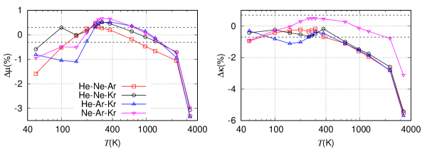
Figure 7: Deviations of viscosities (left) and thermal conductivities (right) of equimolar ternary mixtures reported by Kestin et al. Kes01 (subscript “K”) from those calculated in the present work (subscript “P”), $\Delta C(\%)=(C_{\mbox{\tiny K}}/C_{\mbox{\tiny P}}-1)\times 100$, $C=\mu,\kappa$, dashed lines - uncertainty declared in Ref. Kes01 .

VI.4 Quaternary mixture

Numerical data on viscosity and thermal conductivity of the quaternary He-Ne-Ar-Kr mixture are given in Table 9 for equimolar composition and for four compositions when the molar fraction of one species is 0.1, while that for the rest of species is 0.3. Kestin et al. Kes01 reported the transport coefficients only for the equimolar mixture with the uncertainties of 0.3% and 0.7% for viscosity and thermal conductivity, respectively. Figure 8 shows the deviation of the data by Kestin et al. Kes01 from the present results. In case of viscosity, the deviation is within the uncertainty in the temperature range from 100 K to 1273 K, but it reaches 3.2% at $T=$3273 K. The deviation of the thermal conductivity is larger than that of the viscosity. At high temperatures, the deviation magnitude reaches the value of 5.4%.

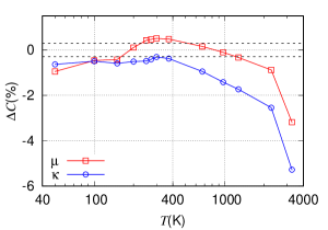
Figure 8: Deviation of viscosity and thermal conductivity of equimolar helium-neon-argon-krypton mixture reported by Kestin et al. (subscript “K”) from those calculated in the present work (subscript “P”), $\Delta C(\%)=(C_{\mbox{\tiny K}}/C_{\mbox{\tiny P}}-1)\times 100$, $C=\mu,\kappa$, dashed lines - uncertainty of thermal conductivity declared in Ref. Kes01 .

Table 9: Viscosity $\mu$ and thermal conductivity $\kappa$ vs. temperature $T$ and molar fractions of helium $x_{1}$, neon $x_{2}$, and argon $x_{3}$ for quaternary mixture He-Ne-Ar-Kr.

	$\mu$($\mu$Pa$\cdot$s)					$\kappa$(mW/(m$\cdot$K))
	$x_{1}=0.25$	0.1	0.3	0.3	0.3	$x_{1}=0.25$	0.1	0.3	0.3	0.3
	$x_{2}=0.25$	0.3	0.1	0.3	0.3	$x_{2}=0.25$	0.3	0.1	0.3	0.3
$T$(K)	$x_{3}=0.25$	0.3	0.3	0.1	0.3	$x_{3}=0.25$	0.3	0.3	0.1	0.3
50.	5.79497	5.55685	5.48530	6.18955	5.99105	8.72551	5.87628	8.39333	10.1887	11.1836
100.	10.6494	10.3394	9.97736	11.3028	11.0007	15.3859	10.6418	14.7101	17.7800	19.5962
200.	19.4088	19.1822	18.4563	20.3206	19.5907	26.3442	18.7734	25.2385	30.0639	33.1505
300.	26.9424	26.8409	25.9352	28.0515	26.7700	35.5593	25.6491	34.1805	40.3717	44.4457
500.	39.5392	39.6151	38.5018	41.0259	38.7355	51.2660	37.2498	49.4763	58.0165	63.7190
800.	55.1166	55.3130	53.9782	57.1462	53.6535	71.3473	51.8548	69.0484	80.7088	88.4801
1000.	64.2867	64.5117	63.0499	66.6619	62.4984	83.4399	60.5585	80.8361	94.4249	103.443
2000.	103.265	103.397	101.427	107.226	100.401	136.290	98.1008	132.394	154.640	169.100
3000.	136.512	136.399	134.052	141.914	132.945	182.624	130.580	177.672	207.661	226.855
5000.	195.118	194.340	191.471	203.176	190.551	266.239	188.514	259.574	303.697	331.317

VII Conclusions

The viscosity and thermal conductivity of multi-component mixtures composed from helium, neon, argon, and krypton in the limit of low density have been calculated on the basis of ab initio potentials over the temperature range from 50 K - 5000 K. The Chapman-Enskog method with the 10th order of approximation has been employed. The relative numerical error does not exceed the value $10^{-6}$ and $10^{-5}$ for the viscosity and thermal conductivity, respectively. However, the relative uncertainty of these coefficients related to the potentials reaches $10^{-3}$. It has been shown that the quantum effects in the interatomic collisions of krypton pair affects the transport coefficients within 0.05% that is about the experimental error reported in Ref. Ber14 . That is why, all calculations have been carried out using the quantum approach to interatomic collisions. Moreover, the present results on pure krypton are closest to the experimental value Ber14 among all previous theoretical works. The viscosity and thermal conductivity of binary, ternary and quaternary mixtures have been compared with other theoretical works showing that the present results are most accurate at the moment. The results data in the present work together with those published previously Cen01 ; Sha118 ; Sha126 ; Bic02 represent the complete database of the viscosity and thermal conductivity of all possible mixtures composed from helium, neon, argon, and krypton over wide ranges of the temperature and mole fractions.

Appendix A Derivation of thermal conductivity expression

To derive the expression (5) of the steady state thermal conductivity of gaseous mixture composed from $K$ species, we depart from Eq.(6.3-50) of the book by Ferziger and Kaper Fer02

$$\kappa=\frac{1}{3}k_{\mbox{\tiny B}}\sum_{i,j=1}^{K}x_{i}x_{j}\int\widetilde{{\boldsymbol{A}}}_{i}\cdot I_{ij}(\widetilde{{\boldsymbol{A}}})\,\mbox{d}^{3}c_{i},$$ (24)

$$\widetilde{{\boldsymbol{A}}}_{i}={\boldsymbol{A}}_{i}-\sum_{l=1}^{K}k_{Tl}{\boldsymbol{D}}_{i}^{l},$$ (25)

where $I_{ij}$ is the linearized collision integral between species $i$ and $j$ Fer02 , $k_{Tl}$ is the thermal diffusion ratio of species $l$ coupled as

$$\sum_{l=1}^{K}k_{Tl}=0.$$ (26)

The vectors ${\boldsymbol{A}}_{i}$ and ${\boldsymbol{D}}_{i}^{l}$ obey the following Boltzmann equations, see Eqs. (6.3-18) and (6.3-19) from the book Fer02 ,

$$\sum_{j=1}^{K}x_{i}x_{j}I_{ij}({\boldsymbol{A}})=\frac{1}{n}f^{M}_{i}\left(\mathscr{C}_{i}^{2}-\frac{5}{2}\right){\boldsymbol{C}}_{i},$$ (27)

$$\sum_{j=1}^{K}x_{i}x_{j}I_{ij}({\boldsymbol{D}}^{l})=\frac{1}{n_{i}}f^{M}_{i}\left(\delta_{il}-\frac{\rho_{i}}{\rho}\right){\boldsymbol{C}}_{i},$$ (28)

$$f_{i}^{M}=n_{i}\left(\frac{m}{2\pi k_{\mbox{\tiny B}}T}\right)^{3/2}e^{-\mathscr{C}^{2}_{i}},$$ (29)

$$\rho_{i}=m_{i}n_{i},\quad\rho=\sum_{i=1}^{K}\rho_{i}.$$ (30)

Combining (26) and (28), we obtain

$$\sum_{j=1}^{K}x_{i}x_{j}I_{ij}\left(\sum_{l=l}^{K}k_{Tl}{\boldsymbol{D}}^{l}\right)=\frac{k_{Ti}}{n_{i}}f^{M}_{i}{\boldsymbol{C}}_{i}.$$ (31)

A summation of (27) and (31) leads to the integral equation for $\widetilde{\boldsymbol{A}}$

$$\sum_{j=1}^{K}x_{i}x_{j}I_{ij}(\widetilde{\boldsymbol{A}})=\frac{1}{n}f^{M}_{i}\left(\mathscr{C}_{i}^{2}-\frac{5}{2}-\frac{k_{Ti}}{x_{i}}\right){\boldsymbol{C}}_{i}.$$ (32)

To solve this equation, the variational principle formulated in Ref. Fer02 is used. First, a trial function ${\boldsymbol{a}}_{i}({\boldsymbol{C}}_{i})$ of the order $N$ is introduced as

$${\boldsymbol{a}}_{i}({\boldsymbol{C}}_{i})=-\frac{15\sqrt{m_{i}}}{4}\sum_{p=1}^{N}{a}_{i}^{(p)}S_{3/2,i}^{(p)}{\boldsymbol{C}}_{i},$$ (33)

where $S_{3/2,i}^{(p)}$ are given by (12). The terms for $p=0$ are omitted because each species is at rest. To find the coefficients $a_{i}^{(p)}$, we need to maximize the functional $g$

$$g=\frac{8}{225k_{\mbox{\tiny B}}T}\sum_{i,j=1}^{K}x_{i}x_{j}\int{{\boldsymbol{a}}}_{i}\cdot I_{ij}({{\boldsymbol{a}}})\,\mbox{d}^{3}c_{i}$$ (34)

under the following constrains

$$\sum_{j=1}^{K}x_{j}\int{{\boldsymbol{a}}}_{i}\cdot I_{ij}({{\boldsymbol{a}}})\,\mbox{d}^{3}c_{i}=\sum_{j=1}^{K}x_{j}\int{{\boldsymbol{a}}}_{i}\cdot I_{ij}(\widetilde{{\boldsymbol{A}}})\,\mbox{d}^{3}c_{i}.$$ (35)

These two conditions guarantee that ${\boldsymbol{a}}_{i}$ tends to $\widetilde{\boldsymbol{A}}$ in the limit $N\to\infty$. Substituting (32) and (33) into (34) and (35), we obtain

$$g=\sum_{i,j=1}^{K}\sum_{p,q=1}^{N}A_{ij}^{(pq)}a_{i}^{(p)}a_{j}^{(q)},$$ (36)

and

$$\sum_{j=1}^{K}\sum_{p,q=1}^{N}A^{(pq)}_{ij}a_{i}^{(p)}a_{j}^{(q)}=\frac{x_{i}}{\sqrt{m_{i}}}a_{i}^{(1)},$$ (37)

respectively. Using the Lagrangian multipliers to combine Eq.(37) with the conditions $\delta\{g\}=0$ where $g$ is given by (36), the system of algebraic equations (7) is derived. A substitution of (37) into (36) results the simple expression of $g$

$$g=\sum_{i=1}^{K}\frac{x_{i}}{\sqrt{m_{i}}}a_{i}^{(1)}.$$ (38)

To obtain the thermal conductivity expression (5), the quantity $\widetilde{\boldsymbol{A}}$ in Eq.(24) is replaced by ${\boldsymbol{a}}_{i}$ in the form (33) and the obtained expression is compared with (34). Then we see

$$\kappa=\frac{75}{8}k_{\mbox{\tiny B}}^{2}Tg.$$ (39)

A substitution of (38) into (39) leads to (5).

References

References

- (1) E. L. Tipton, R. V. Tompson, and S. K. Loyalka, “Chapman-Enskog solutions to arbitrary order in Sonine polynomials II: Viscosity in a binary, rigid-sphere, gas mixture,” Eur. J. Mech. B-Fluids 28, 335–352 (2009).
- (2) E. L. Tipton, R. V. Tompson, and S. K. Loyalka, “Chapman-Enskog solutions to arbitrary order in Sonine polynomials III: Diffusion, thermal diffusion, and thermal conductivity in a binary, rigid-sphere, gas mixture,” Eur. J. Mech. B-Fluids 28, 353–386 (2009).
- (3) R. V. Tompson, E. L. Tipton, and S. K. Loyalka, “Chapman-Enskog solutions to arbitrary order in Sonine polynomials IV: Summational expressions for the diffusion- and thermal conductivity-related bracket integrals,” Eur. J. Mech. B-Fluids 28, 695–721 (2009).
- (4) R. V. Tompson, E. L. Tipton, and S. K. Loyalka, “Chapman-Enskog solutions to arbitrary order in Sonine polynomials V: Summational expressions for the viscosity-related bracket integrals,” Eur. J. Mech. B-Fluids 29, 153–179 (2010).
- (5) B. Song, X. Wang, J. Wu, and Z. Liu, “Prediction of transport properties of pure noble gases and some of their binary mixtures by ab initio calculations,” Fluid Phase Equilibria 290, 55–62 (2010).
- (6) F. Sharipov and V. Benites, “Transport coefficients of helium-argon mixture based on ab initio potential,” J. Chem. Phys. 143, 154 104 (2015).
- (7) F. Sharipov and V. Benites, “Transport coefficients of helium-neon mixtures at low density computed from ab initio potentials,” J. Chem. Phys. 147, 224 302 (2017).
- (8) F. Sharipov and V. Benites, “Transport coefficients of argon and its mixtures with helium and neon at low density based ab initio potentials,” Fluid Phase Equilibria 498, 23–32 (2019).
- (9) S. Chapman and T. G. Cowling, The Mathematical Theory of Non-Uniform Gases (University Press, Cambridge, 1970), 3 edn.
- (10) J. H. Ferziger and H. G. Kaper, Mathematical Theory of Transport Processes in Gases (North-Holland Publishing Company, Amsterdam, 1972).
- (11) J. Kestin, K. Knierim, E. A. Mason, B. Najafi, S. T. Ro, and M. Waldman, “Equilibrium and transport properties of the noble gases and their mixture at low densities,” J. Phys. Chem. Ref. Data 13, 229–303 (1984).
- (12) S. K. Loyalka, “Velocity slip coefficient and the diffusion slip velocity for a multicomponent gas mixture,” Phys. Fluids 14, 2599–2604 (1971).
- (13) G. Ben-Dor, T. Elperin, and B. Krasovitov, “Numerical analysis of the effects of temperature and concentration jumps on transient evaporation of moderately large (0.01 less than or similar to Kn less than or similar to 0.3) droplets in non-isothermal multicomponent gaseous mixtures,” Heat and Mass Transfer 39, 157–166 (2003).
- (14) L. Szalmas, “Heat transfer in ternary rarefied gas mixtures between two parallel plates,” Eur. J. Mech. B-Fluids 57, 152–158 (2016).
- (15) A. Yakunchikov and V. Kosyanchuk, “Numerical investigation of gas separation in the system of filamentswith different temperatures,” Int. J. Heat Mass Trans. 138, 144–151 (2019).
- (16) F. Sharipov, Rarefied Gas Dynamics. Fundamentals for Research and Practice (Wiley-VCH, Berlin, 2016).
- (17) A. Frezzotti, G. Ghiroldi, and L. Gibelli, “Rarefied gas mixtures flows driven by surface absorption,” Vacuum 86, 1731–1738 (2012).
- (18) S. Naris, D. Valougeorgis, D. Kalempa, and F. Sharipov, “Flow of gaseous mixtures through rectangular microchannels driven by pressure, temperature and concentration gradients,” Phys. Fluids 17, 100 607 (2005).
- (19) F. Sharipov and J. L. Strapasson, “Benchmark problems for mixtures of rarefied gases. I. Couette flow,” Phys. Fluids 25, 027 101 (2013).
- (20) M. T. Ho, L. Wu, I. Graur, Y. Zhang, and J. M. Reese, “Comparative study of the Boltzmann and McCormack equations for Couette and Fourier flows of binary gaseous mixtures,” Int. J. Heat Mass Transfer 96, 29–41 (2016).
- (21) D. Valougeorgis, M. Vargas, and S. Naris, “Analysis of gas separation, conductance and equivalent single gas approach for binary gas mixture flow expansion through tubes of various lengths into vacuum,” Vacuum 128, 1–8 (2016).
- (22) B. Goshayeshi, E. Roohi, and S. Stefanov, “A novel simplified Bernoulli trials collision scheme in the direct simulation Monte Carlo with intelligence over particle distances,” Phys. Fluids 27, 107 104 (2015).
- (23) F. Sharipov and D. Kalempa, “Velocity slip and temperature jump coefficients for gaseous mixtures. III. Diffusion slip coefficient,” Phys. Fluids 16, 3779–3785 (2004).
- (24) F. Sharipov, “Data on the velocity slip and temperature jump on a gas-solid interface,” J. Phys. Chem. Ref. Data 40, 023 101 (2011).
- (25) F. Sharipov and D. Kalempa, “Velocity slip and temperature jump coefficients for gaseous mixtures. IV. Temperature jump coefficient,” Int. J. Heat Mass Transfer 48, 1076–1083 (2005).
- (26) R. S. Brokaw, “Approximate formulas for the viscosity and thermal conductivity of gas mixtures. II,” J. Chem. Phys. 42, 1140–1146 (1965).
- (27) K. Singh and N. Sood, “Viscosity and thermal conductivity of gas mixtures,” Indian J. Pure Appl. Phys. 41, 121–127 (2003).
- (28) J. Avsec and M. Oblak, “Thermal Conductivity, Viscosity, and Thermal Diffusivity Calculation for Binary and Ternary Mixtures,” J. Thermophysics and Heat Transfer 18, 379–387 (2004).
- (29) R. Aziz, A. Janzen, and M. Moldover, “Ab-initio calculations for helium: a standard for transport property measurements,” Phys. Rev. Lett. 74, 1586–1589 (1995).
- (30) S. M. Cybulski and R. R. Toczylowski, “Ground state potential energy curves for He2, Ne2, Ar2, He-Ne, He-Ar, and Ne-Ar: A coupled-cluster study,” J. Chem. Phys. 111, 10 520–10 528 (1999).
- (31) T. P. Haley and S. M. Cybulski, “Ground state potential energy curves for He-Kr, Ne-Kr, Ar-Kr, and Kr2: Coupled-cluster calculations and comparison with experiment,” J. Chem. Phys. 119, 5487–5496 (2003).
- (32) J. Cacheiro, B. Fernández, D. Marchesan, S. Coriani, C. Hättig, and A. Rizzo, “Coupled cluster calculations of the ground state potential and interaction induced electric properties of the mixed dimers of helium, neon and argon,” Mol. Phys. 102, 101–110 (2004).
- (33) R. Hellmann, E. Bich, and E. Vogel, “Ab initio potential energy curve for the neon atom pair and thermophysical properties of the dilute neon gas. I. Neon-neon interatomic potential and rovibrational spectra,” Mol. Phys. 106, 133–140 (2008).
- (34) K. Patkowski and K. Szalewicz, “Argon pair potential at basis set and excitation limits,” J. Chem. Phys. 133, 094 304 (2010).
- (35) M. Przybytek, W. Cencek, J. Komasa, G. Łach, B. Jeziorski, and K. Szalewicz, “Relativistic and quantum electrodynamics effects in the helium pair potential,” Phys. Rev. Lett. 104, 183 003 (2010), Erratum in Phys. Rev. Lett. 108 , 129902 (2012).
- (36) W. Cencek, M. Przybytek, J. Komasa, J. B. Mehl, B. Jeziorski, and K. Szalewicz, “Effects of adiabatic, relativistic, and quantum electrodynamics interactions on the pair potencial and thermophysical properties of helium,” J. Chem. Phys. 136, 224 303 (2012).
- (37) B. Jäger, R. Hellmann, E. Bich, and E. Vogel, “Ab initio pair potential energy curve for the argon atom pair and thermophysical properties of the dilute argon gas. I. Argon-argon interatomic potential and rovibrational spectra,” Mol. Phys. 107, 2181–2188 (2009), erratum in Mol. Phys. 108, 105 (2010).
- (38) B. Jäger, R. Hellmann, E. Bich, and E. Vogel, “State-of-the-art ab initio potential energy curve for the krypton atom pair and thermophysical properties of dilute krypton gas,” J. Chem. Phys. 144, 114 304 (2016).
- (39) B. Jäger and E. Bich, “Thermophysical properties of krypton-helium gas mixtures from ab initio pair potentials,” J. Chem. Phys. 146, 214 302 (2017).
- (40) L. D. Landau and E. M. Lifshitz, Fluid Mechanics (Pergamon, New York, 1989).
- (41) C. Muckenfuss and C. Curtiss, “Thermal conductivity of multicomponent gas mixtures,” J. Chem. Phys. 29, 1273–1277 (1958).
- (42) F. Meeks, T. Cleland, K. Hutchinson, and W. Taylor, “On the quantum cross sections in dilute gases,” J. Chem. Phys. 100, 3813–3820 (1994), erratum in J.Chem.Phys. 103, 1239 (1994).
- (43) J. Joachain, Quantum Collision Theory (North-Holland Publishing Company, Amsterdam, 1975).
- (44) B. Shizgal, Spectral Methods in Chemistry and Physics (Springer, 2015).
- (45) P. J. Mohr, D. B. Newell, and B. N. Taylor, “CODATA Recommended Values of the Fundamental Physical Constants: 2014,” J. Phys. Chem. Ref. Data 45, 043 102 (2016).
- (46) J. Meija, T. B. Coplen, M. Berglund, W. A. Brand, P. De Bievre, M. Groening, N. E. Holden, J. Irrgeher, R. D. Loss, T. Walczyk, and T. Prohaska, “Atomic weights of the elements 2013 (IUPAC Technical Report),” Pure Appl. Chem. 88, 265–291 (2016).
- (47) E. Bich, R. Hellmann, and E. Vogel, “ Ab initio potential energy curve for the helium atom pair and thermophysical properties of the dilute helium gas. II. Thermophysical standard values for low-density helium,” Mol. Phys. 105, 3035–3049 (2007).
- (48) R. Berg and M. Moldover, “Recommended viscosities of 11 Dilute Gases at 25∘ C,” J. Phys. Chem. Ref. Data 41, 043 104 (2012).
- (49) R. F. Berg and W. C. Burton, “Noble gas viscosities at 25∘ C,” Mol. Phys. 111, 195–199 (2013).
- (50) E. Bich, R. Hellmann, and E. Vogel, “ Ab initio potential energy curve for the neon atom pair and thermophysical properties for the dilute neon gas. II. Thermophysical properties for low-density neon,” Mol. Phys. 106, 813–825 (2008).