Bonus Properties of States of Low Energy

Rudrajit Banerjee and Max Niedermaier

Department of Physics and Astronomy
University of Pittsburgh, 100 Allen Hall
Pittsburgh, PA 15260, USA

Abstract

States of Low Energy (SLE) are exact Hadamard states defined on arbitrary Friedmann-Lemaître spacetimes. They are constructed from a fiducial state by minimizing the Hamiltonian’s expectation value after averaging with a temporal window function. We show the SLE to be expressible solely in terms of the (state independent) commutator function. They also admit a convergent series expansion in powers of the spatial momentum, both for massive and for massless theories. In the massless case the leading infrared behavior is found to be Minkowski-like for all scale factors. This provides a new cure for the infrared divergences in Friedmann-Lemaître spacetimes with accelerated expansion. In consequence, massless SLE are viable candidates for pre-inflationary vacua and in a soluble model are shown to entail a qualitatively correct primordial power spectrum.

1.  Introduction

For perturbatively defined quantum field theories on globally hyperbolic spacetimes there is a general consensus that the free state on which perturbation theory is based should be a Hadamard state. By-and-large the Hadamard property is necessary and sufficient for the existence of Wick powers of arbitrary order and hence for the perturbative series to be termwise well-defined at any order, see [1, 8] for recent accounts. On the other hand, Hadamard states are surprisingly difficult to construct concretely [2, 11, 14] even for background spacetimes with some degree of symmetry (other than maximal). The well-known adiabatic iteration [3] has certain characteristics necessary for the Hadamard property built in, but is not convergent and cannot be fruitfully extended to small spatial momenta. The iteration can, however, serve as a conduit to establish the existence of states locally indistinguishable from Hadamard states [11].

An important class of backgrounds are generic Friedmann-Lemaître cosmologies, where a construction of exact Hadamard states has become available only relatively recently [5]. These States of Low Energy (SLE) arise by minimizing the Hamiltonian’s expectation value after averaging with a temporal window function $f$. The temporal averaging is crucial and avoids the pathologies [9] of the earlier instantaneous diagonalization procedure. The construction of a SLE takes some fiducial solution $S$ of the homogeneous wave equation a starting point, considers arbitrary Bogoliubov transformations thereof, and then minimizes the temporal average of the energy with respect to them. Olbermann’s theorem [5] states that (for a massive free quantum field theory an a Friedmann-Lemaître background) the minimizing solution $T[S]$ gives rise to an exact Hadamard state. For given $S$ the minimizer $T[S]$ is unique up to a phase.

Here we show that the SLE have a number of bonus properties that make them mathematically even more appealing and which also render them good candidates for vacuum-like states in a pre-inflationary period. Specifically, we show that for a given temporal averaging function $f$:

• The SLE two-point function $W[S]$ based on a fiducial solution $S$ is a Bogoliubov invariant, $W[aS+bS^{\ast}]=W[S]$, with $a,b\in\mathbb{C}$ , $|a|^{2}-|b|^{2}=1$. Hence $W[S]$ is independent of the choice of fiducial solution $S$.

• The minimization over Bogoliubov parameters relative to a given $S$ can be replaced by a minimization over initial data, without reference to any fiducial solution. The resulting expression for the SLE solution $T[\Delta]$ is fully determined by the (Bogoliubov invariant and state independent) commutator function $\Delta$, making manifest the uniqueness of the SLE. The minimization over initial data has a natural interpretation in the Schrödinger picture.

• The SLE solution admits a convergent series expansion in powers of the (modulus of the) spatial momentum, both for massive and for massless theories.

• In the massless case the leading infrared behavior is Minkowski-like for all cosmological scale factors. This provides a new cure for the long standing infrared divergences in Friedmann-Lemaître backgrounds with accelerated expansion [22].

• The modulus square of an SLE solution admits an asymptotic expansion in inverse odd powers of the (modulus of the) spatial momentum, which is independent of the window function $f$. The coefficients of the expansion are local, recursively computable, and generalize the heat kernel coefficients. The asymptotics of the phase is governed by single integrals of the same coefficients. This short cuts the detour via the adiabatic expansion.

Since linearized cosmological perturbations are described by massless free fields, the property (d) renders SLE a legitimate choice for a vacuum-like state in the early universe. Specifically, we argue that within the standard paradigm (classical Friedmann-Lemaître backgrounds with selfinteracting scalar field) inflation must have been preceded by a period of non-accelerated expansion, for which the type with kinetic energy domination is mathematically preferred. The occurrence of the Bunch-Davies vacuum at the onset of inflation then requires extreme fine tuning. In contrast, postulating a SLE for the primordial vacuum in the pre-inflationary phase is shown to automatically produce a qualitatively realistic power spectrum at the end of inflation.

The paper is organized as follows. After introducing the SLE in the Heisenberg and the Schrödinger pictures we establish properties (a) and (b) in Sections 2.2 and 2.3, respectively. The existence of a convergent small momentum expansion is shown in Section 3.1, with the massless case detailed in Section 3.2. For large momentum, the existence of the WKB type expansion governed by generalized heat kernel coefficients is shown in Section 4. Finally, we study the viability of massless SLE as pre-inflationary vacua in Section 5.

2.  SLE in the Heisenberg and Schrödinger pictures

A State of Low Energy (SLE) was originally defined in the Heisenberg picture by minimizing with respect to Bogoliubov parameters relating the corresponding solution of the wave equation to a reference solution $S$. As such, the SLE construction depends on the reference solution. Here we show that the SLE two-point function (which specifies the state completely) is independent of $S$. Next, the energy functional in the Schrödinger picture is naturally regarded as a function of the wave function’s initial data. By minimizing over initial data an alternative explicit expression for the SLE is obtained, which depends only on the (Bogoliubov invariant and state independent) commutator function.

2.1  Homogeneous pure quasifree states in Heisenberg and Schrödinger pictures

Throughout, the background geometry will be a $1\!+\!d$ dimensional, spatially flat Friedmann-Lemaître (FL) cosmology with line element

$$ds^{2}=-\bar{N}(t)^{2}dt^{2}+a(t)^{2}\delta_{ij}dx^{i}dx^{j}\,,$$ (2.1)

where $\bar{N}:\mathbb{R}_{+}\rightarrow\mathbb{R}_{+}$ is the lapse function, $a:\mathbb{R}_{+}\rightarrow\mathbb{R}_{+}$ is the cosmological scale factor, and $x^{i},i=1,\ldots,d$ are adapted spatial coordinates. The form of the line element (2.1) is preserved under ${\rm Diff}[t_{i},t_{f}]\times{\rm ISO}(d)$ transformations, where ${\rm Diff}[t_{i},t_{f}]$ are endpoint preserving reparameterizations of some time interval $[t_{i},t_{f}]$, $0<t_{i}<t_{f}<\infty$, and the Euclidean group ${\rm ISO}(d)$ acts via global spatial diffeomorphisms connected to the identity. On this background we consider a scalar field $\chi:\mathbb{R}_{+}\times\mathbb{R}^{d}\rightarrow\mathbb{R}$, which is minimally coupled and initially selfinteracting with potential $U(\chi)$. Under the temporal reparameterizations $a(t)$ and $\chi(t,x)$ transform as scalars, while $\bar{N}(t)$ and $\bar{n}(t):=\bar{N}(t)/a(t)^{d}$ are temporal densities, $\bar{n}^{\prime}(t^{\prime})=\bar{n}(t)/|\partial t^{\prime}/\partial t|$, etc.. This is such that $\int_{t_{i}}^{t_{f}}\!dt\bar{N}(t)a(t)^{p}=\int_{t_{i}}^{t_{f}}\!dt\,\bar{n}(t)a(t)^{p+d}$ is invariant for any $p$. Next, we expand the minimally coupled scalar field action on $[t_{i},t_{f}]\times\mathbb{R}^{d}$ around a spatially homogeneous background scalar $\varphi(t)$ to quadratic order in the fluctuations $\phi(t,x):=\chi(t,x)-\varphi(t)$. This gives a leading term $\bar{S}^{\varphi}$ (multiplied by a spatial volume term) whose field equation is one of the evolution equations for a FL cosmology. For $\varphi(t)$ solving it (with prescribed $a(t)$) the term linear in the $\phi$ reduces to a boundary term and may be omitted. The quadratic piece reads

$$S^{\phi}=\frac{1}{2}\int_{t_{i}}^{t_{f}}\!dt\int_{\Sigma}\!dx\,\Big{\{}\frac{1}{\bar{n}(t)}(\partial_{t}\phi)^{2}-\bar{n}(t)a(t)^{2d}U^{\prime\prime}(\varphi)\phi^{2}-\bar{n}(t)a(t)^{2d-2}\partial_{i}\phi\delta^{ij}\partial_{j}\phi\Big{\}}\,.$$ (2.2)

So far, $\varphi$ is for prescribed $a(t)$ a solution of $\-\partial_{t}(\bar{n}^{-1}\partial_{t}\varphi)+\epsilon_{g}\bar{n}a^{2d}U^{\prime}(\varphi)=0$, but $a(t)$ itself is unconstrained. As far as the homogeneous background is concerned one could now augment the missing gravitational dynamics by the other FL field equations. This would turn $a(t),\varphi(t)$ into a solution of the Einstein equations and classical backreaction effects would be taken into account in the homogeneous sector. The standard “Quantum Field Theory (QFT) on curved background” viewpoint, on the other hand, treats the geometry as external, in which case (2.2) adheres to the minimal coupling principle only if $U^{\prime\prime}(\varphi)=m_{0}^{2}$ is identified with a constant mass squared. In order to be able to switch back and forth between both settings we shall view $U^{\prime\prime}(\varphi)=m(t)^{2}$ formally as a time dependent mass and carry it along, specifying its origin only when needed. In the field equations $\delta S^{\phi}/\delta\phi=0$ a spatial Fourier transform is natural, $\phi(t,x)=\int\!dp(2\pi)^{-d}e^{ipx}\phi(t,p)$. Then $-\partial_{i}\delta^{ij}\partial_{j}$ acts like $p^{2}:=p_{i}\delta^{ij}p_{i}$, which converts the field equation into an ordinary differential equation for each $p$ mode, viz $[(\bar{n}^{-1}\partial_{t})^{2}+a(t)^{2d}m(t)^{2}+a(t)^{2d-2}p^{2}]\phi(t,p)=0$.

Homogeneous pure quasifree states. On a FL background geometry there are, in general, infinitely many physically viable vacuum-like states for a QFT. A vacuum-like state is in particular a “homogeneous pure quasifree” state. A “state” is normally defined algebraically as a positive linear functional over the Weyl algebra [1]. For the present purposes a “state” can be identified with the set of multi-point functions it gives rise to. Then “quasifree” means that all odd $n$-point functions in the state vanish while the even $n$-point functions can be expressed in terms of the two-point function $W(t,x;t^{\prime},x^{\prime})$ via Wick’s theorem. Being a “state” entails certain properties of the two-point function that allow one to realize it via the Gelfand-Naimark-Segal (GNS) construction in the form $(\Omega,u(t,x)u(t^{\prime},x^{\prime})\Omega)$, for field operators $u(t,x)$ on vectors $\Omega$ in the reconstructed state space. “Pure” means that $\Omega$ cannot be written as a convex combination of other states. Finally, for a spatially flat FL background, “homogeneous” just means “translation invariant”, i.e. $W(t,x;t^{\prime},x^{\prime})$ depends only on $x\!-\!x^{\prime}$.

The GNS reconstructed field operators $u(t,x)$ turn out to coincide with the Heisenberg field operators $\phi(t,x)$ (which are denoted by the same symbol as the classical field, as the latter will no longer occur.) The GNS vector $\Omega$ turns out to correspond to a Fock vacuum $|0_{T}\rangle$, annihilated by annihilation operators defined by a mode expansion of the Heisenberg field operator

$$\phi(t,x)=\int\!\frac{dp}{(2\pi)^{d}}\big{[}T_{p}(t){\bf a}_{T}(p)e^{ipx}+T_{p}(t)^{*}{\bf a}_{T}^{*}(p)e^{-ipx}\big{]}\,,$$

$$\big{[}{\bf a}_{T}(p),{\bf a}_{T}^{*}(p^{\prime})]=(2\pi)^{d}\delta(p-p^{\prime})\,,\quad{\bf a}_{T}(p)|0_{T}\rangle=0\,,$$ (2.3)

where $T_{p}(t)$ is a complex solution of the above classical wave equation, and in the massless case $p=0$ needs to be excluded in the definition of $|0_{T}\rangle$. In order for the equal time commutation relations $[\phi(t,p),(\bar{n}^{-1}\partial_{t}\phi)(t,p^{\prime})]=i(2\pi)^{d}\delta(p+p^{\prime})$ to hold, this solution must obey the Wronskian normalization condition $(\bar{n}^{-1}\partial_{t}T_{p})(t)T_{p}(t)^{*}-(\bar{n}^{-1}\partial_{t}T_{p})(t)^{*}T_{p}(t)=-i$. Then

$$W(t,x;t^{\prime},x^{\prime})=\langle 0_{T}|\phi(t,x)\phi(t^{\prime},x^{\prime})|0_{T}\rangle=\int\!\frac{dp}{(2\pi)^{d}}\,T_{p}(t)\,T_{p}(t^{\prime})^{\ast}\,e^{ip(x-x^{\prime})}\,.$$ (2.4)

One sees that modulo phase choices a “homogeneous pure quasifree” state is characterized by a choice of Wronskian normalized solution $T_{p}(t)$ of the wave equation or, equivalently, by a choice of Fock vacuum $|0_{T}\rangle$ via (2.1).

Conventions. We briefly comment on our choice of conventions. In (2.1) often the ${\bf a}_{T}^{*}(p)$ is paired with $T_{p}(t)$ not with $T_{p}(t)^{*}$. Then the sign in the Wronskian normalization condition has to be flipped correspondingly. More importantly, we seek to preserve temporal reparameterization invariance by carrying the lapse-like $\bar{n}(t)=\bar{N}(t)/a(t)^{d}$ along. Since in the wave equation $\bar{n}$ only occurs in the combination $\bar{n}^{-1}\partial_{t}$, it is convenient to introduce a new time function

$$\tau:=\int^{t}_{t_{i}}\!dt^{\prime}\bar{n}(t^{\prime})\,,\quad\partial_{\tau}=\bar{n}(t)^{-1}\partial_{t}\,,$$ (2.5)

for some $t_{i}$. Note that $\tau(t)=\tau^{\prime}(t^{\prime})$ is a scalar under reparameterizations $t^{\prime}=\chi^{0}(t)$ of the coordinate time $t$, and that $d\tau=dt\bar{n}(t)$, $\bar{n}(t)^{-1}\delta(t,t^{\prime})=\delta(\tau,\tau^{\prime})$ are likewise invariant. Here $t^{\prime}=\chi^{0}(t)$ with $\chi^{0}(t_{i})=t_{i}<t_{f}=\chi^{0}(t_{f})$ must be strictly increasing to qualify as a diffeomorphism. We write $a(\tau)$ for the cosmological scale factor viewed as a function of $\tau$ rather than $t$, and similarly for $m(\tau)$ as well as $T_{p}(\tau)$. The defining relations for $T_{p}(\tau)$ then read

$$\big{[}\partial_{\tau}^{2}+\omega_{p}(\tau)^{2}]T_{p}(\tau)=0\,,\quad\omega_{p}(\tau)^{2}:=a(\tau)^{2d}m(\tau)^{2}+p^{2}a(\tau)^{2d-2}\,,$$

$$\partial_{\tau}T_{p}\,T_{p}^{*}-\partial_{\tau}T_{p}^{*}\,T_{p}=-i\,.$$ (2.6)

This setting has the advantage that the results in different time variables can be obtained by specialization:

Cosmological time $$: \bar{n}(t)=a(t)^{-d}\;\mbox{gauge, i.e.}\;\bar{N}(t)=1\,,$$

Conformal time $$: \bar{n}(t)=a(t)^{1-d}\;\mbox{gauge, i.e.}\;\bar{N}(t)=a(t)\,,$$

Proper time $$: \bar{n}(t)=1\;\mbox{gauge, i.e.}\;\bar{N}(t)=a(t)^{d}\,.$$ (2.7)

The first two gauges are standard; commonly one writes $\eta$ for $t$ in conformal time gauge. The last gauge is the FL counterpart of the proper time gauge $\partial_{t}n(t,x)=0$ often adopted for the evolution of generic foliated spacetimes.

Generally, $(\bar{n}^{-1}\partial_{t})^{2}=\bar{n}^{-2}(\partial_{t}^{2}-\bar{n}^{-1}\partial_{t}\bar{n}\partial_{t})$ and the first order term can be removed by the redefinition $T_{p}(t)=\bar{n}(t)^{1/2}\chi_{p}(t)$. This gives

$$\big{[}\partial_{t}^{2}+\bar{n}(t)^{2}\omega_{p}(t)^{2}+\bar{s}(t)\big{]}\chi_{p}(t)=0\,,$$

$$\bar{s}(t):=\frac{1}{2}\frac{\partial_{t}^{2}\bar{n}}{\bar{n}}-\frac{3}{4}\Big{(}\frac{\partial_{t}\bar{n}}{\bar{n}}\Big{)}^{2}\,,$$

$$\partial_{t}\chi_{p}\chi_{p}^{*}-(\partial_{t}\chi_{p})^{*}\chi_{p}=-i\,.$$ (2.8)

In conformal time, $\bar{n}(t)=a(t)^{1-d}$ the coefficient of $p^{2}$ is unity and after renaming $t$ into $\eta$ one has

$$\Big{[}\partial_{\eta}^{2}+p^{2}+\frac{m(\eta)^{2}}{a(\eta)^{2}}+\bar{s}(\eta)\Big{]}\chi_{p}(\eta)=0\,,$$

$$\bar{s}(\eta):=-\frac{d\!-\!1}{2}\frac{\partial_{\eta}^{2}a}{a}-\frac{(d\!-\!3)(d\!-\!1)}{4}\Big{(}\frac{\partial_{\eta}a}{a}\Big{)}^{2}\,,$$

$$\partial_{\eta}\chi_{p}\chi_{p}^{*}-(\partial_{\eta}\chi_{p})^{*}\chi_{p}=-i\,.$$ (2.9)

We shall occasionally discretize the flat spatial sections of (2.1), which are isometric to $\mathbb{R}^{d}$, in order to regularize momentum integrals. A hypercubic lattice $\Lambda=\{x=a_{s}(n_{1},\ldots,n_{d}),\;n_{j}=0,\ldots,L\!-\!1\}$ suffices, with dual lattice $\hat{\Lambda}=\{p=\frac{2\pi}{a_{s}L}(n_{1},\ldots,n_{d})\,,\;n_{j}=0,\ldots,L\!-\!1\}$, where $a_{s}>0$ is the spatial lattice spacing and $L\in\mathbb{N}$ is large. A discretized Fourier transform $\hat{f}:\hat{\Lambda}\rightarrow\mathbb{C}$ is defined for real valued functions $f:\Lambda\rightarrow\mathbb{R}$ with periodic boundary conditions $f(x+a_{s}L\hat{\imath})=f(x)$, $i=1,\ldots,d$. The direct and inverse transforms read

$$\hat{f}(p)=a_{s}^{d}\sum_{x\in\Lambda}e^{-ipx}f(x)\,,\quad f(x)=\frac{1}{(a_{s}L)^{d}}\sum_{p\in\hat{\Lambda}}e^{ip\cdot x}\hat{f}(p)\,.$$ (2.10)

The continuum limit is taken by first sending $L\rightarrow\infty$, which converts $(a_{s}L)^{-d}\sum_{p\in\hat{\Lambda}}$ into an integral $(2\pi)^{-d}\int\!d^{d}p$ over the Brillouin zone $p\in[-\pi/a_{s},\pi/a_{s}]^{d}$, and then taking $a_{s}\rightarrow 0$. As usual, the lattice Laplacian $\Delta_{s}$ acts by multiplication in Fourier space

$$-\Delta_{s}\,e^{ip\cdot x}=\hat{p}^{2}e^{ip\cdot x}\,,\quad\hat{p}^{2}:=\sum_{j=1}^{d}\hat{p}_{j}^{2}=\frac{4}{a_{s}^{2}}\sum_{j=1}^{d}\sin^{2}\Big{(}\frac{p_{j}a_{s}}{2}\Big{)}\,.$$ (2.11)

Unless confusing we shall set $a_{s}\!=\!1$ and omit the ‘hat’ on the Fourier transformed functions.

Heisenberg picture. Time evolution in the Heisenberg picture is generated by the canonical Hamiltonian derived from (2.2) with the field operators (2.1) inserted. After Fourier decomposition this leads to

$$\mathbb{H}(\tau)=\int\!\frac{dp}{(2\pi)^{d}}\,\mathbb{H}_{p}(\tau)\,,\makebox[28.45274pt]{ }\omega_{p}(\tau)^{2}:=m(\tau)^{2}a(\tau)^{2d}+p^{2}a(\tau)^{2d-2}\,,$$

$$\mathbb{H}_{p}(\tau)=\frac{1}{2}|\pi(\tau,p)|^{2}+\frac{1}{2}\omega_{p}(\tau)^{2}|\phi(\tau,p)|^{2}$$ (2.12)

$$\quad=\frac{1}{2}\big{(}|\partial_{\tau}T_{p}|^{2}+\omega_{p}(\tau)^{2}|T_{p}|^{2}\big{)}\big{(}{\bf a}_{T}(-p){\bf a}_{T}^{*}(-p)+{\bf a}_{T}^{*}(p){\bf a}_{T}(p)\big{)}$$

$$\quad+\frac{1}{2}\big{(}(\partial_{\tau}T_{p})^{2}+\omega_{p}(\tau)^{2}T_{p}^{2}\big{)}{\bf a}_{T}(-p){\bf a}_{T}(p)+\frac{1}{2}\big{(}(\partial_{\tau}T_{p}^{*})^{2}+\omega_{p}(\tau)^{2}(T_{p}^{*})^{2}\big{)}{\bf a}_{T}^{*}(p){\bf a}_{T}^{*}(-p)\,.$$

In particular

$$\partial_{\tau}\phi(\tau,p) \!=\! i[\mathbb{H}(\tau),\phi(\tau,p)]=\pi(\tau,p)\,,$$

$$\partial_{\tau}\pi(\tau,p) \!=\! i[\mathbb{H}(\tau),\pi(\tau,p)]=-\omega_{p}(\tau)^{2}\phi(\tau,p)\,,$$ (2.13)

are the Heisenberg picture evolution equations. For later use we prepare their solution in terms of the (real, anti-symmetric) commutator function $\Delta_{p}(\tau^{\prime},\tau)$ defined by

$$\big{[}\partial_{\tau}^{2}+\omega_{p}(\tau)^{2}\big{]}\Delta_{p}(\tau,\tau_{0})=0=\big{[}\partial_{\tau_{0}}^{2}+\omega_{p}(\tau_{0})^{2}\big{]}\Delta_{p}(\tau,\tau_{0})\,,$$

$$\Delta_{p}(\tau,\tau_{0})=-\Delta_{p}(\tau_{0},\tau)\,,\quad\partial_{\tau}\Delta_{p}(\tau,\tau_{0})\big{|}_{\tau=\tau_{0}}=1\,.$$ (2.14)

The terminology of course refers to the relations

$$i[\phi(\tau,p),\phi(\tau_{0},p_{0})] \!=\! (2\pi)^{d}\delta(p+p_{0})\Delta_{p}(\tau,\tau_{0})\,,$$

$$\Delta_{p}(\tau,\tau_{0}) := i\big{(}T_{p}(\tau)T_{p}(\tau_{0})^{*}-T_{p}(\tau)^{*}T_{p}(\tau_{0})\big{)}\,,$$ (2.15)

so that $\partial_{\tau}\Delta_{p}(\tau,\tau_{0})|_{\tau=\tau_{0}}=1$ codes the equal time commutation relations. Note that any other Wronskian normalized complex solution defines the same commutator function, see Lemma 2.3. The solution of the evolution equations (2.1) then reads

$$\phi(\tau,p) \!=\! \Delta_{p}(\tau,\tau_{0})\pi(\tau_{0},p)-\partial_{\tau_{0}}\Delta_{p}(\tau,\tau_{0})\phi(\tau_{0},p)\,,$$

$$\pi(\tau,p) \!=\! \partial_{\tau}\Delta_{p}(\tau,\tau_{0})\pi(\tau_{0},p)-\partial_{\tau}\partial_{\tau_{0}}\Delta_{p}(\tau,\tau_{0})\phi(\tau_{0},p)\,.$$ (2.16)

The central object later on will be the Hamilton operator (2.1) averaged with a smooth positive window function $f(\tau)^{2}$ of compact support in $(\tau_{i},\tau_{f})$. We write

$$\int\!\!d\tau f(\tau)^{2}\,\mathbb{H}_{p}(\tau) \!=\! {\cal E}_{p}[T]\big{(}{\bf a}_{T}(-p){\bf a}_{T}^{*}(-p)+{\bf a}_{T}^{*}(p){\bf a}_{T}(p)\big{)}$$ (2.17)

$$+ {\cal D}_{p}[T]\,{\bf a}_{T}(-p){\bf a}_{T}(p)+{\cal D}_{p}[T]^{*}\,{\bf a}_{T}^{*}(p){\bf a}_{T}^{*}(-p)\,,$$

with

$${\cal E}_{p}[T]\! \!:=\! \!\frac{1}{2}\int\!d\tau\,f(\tau)^{2}\,\Big{\{}|\partial_{\tau}T_{p}|^{2}+\omega_{p}(\tau)^{2}|T_{p}|^{2}\Big{\}}>|{\cal D}_{p}[T]|\,,$$

$${\cal D}_{p}[T]\! \!:=\! \!\frac{1}{2}\int\!d\tau f(\tau)^{2}\,\Big{\{}(\partial_{\tau}T_{p})^{2}+\omega_{p}(\tau)^{2}T_{p}^{2}\Big{\}}\,.$$ (2.18)

The above formulation preserves temporal reparameterization invariance through the use of $\tau$ from (2.5). As a consequence, the solutions of the wave equation (2.1) can be interpreted as functions of the coordinate time $t$ with a functional dependence on $\bar{n}$. We shall occasionally do so and then (by slight abuse of notation) keep the function symbols, writing $T_{p}(\tau)=T_{p}(t)$, etc.. When fixing a gauge as in (2.1) one will however normally absorb additional powers of $a(t)$ into a redefined averaging function and frequency. Specifically,

$${\cal E}_{p}[T]=\!\frac{1}{2}\int\!dt\,f(t)^{2}\bar{n}(t)^{-1}\,\Big{\{}|\partial_{t}T_{p}|^{2}+(\bar{n}(t)\omega_{p}(t))^{2}|T_{p}|^{2}\Big{\}}\,,$$ (2.19)

motivates

$$f^{\rm cosm}(t)^{2} := f(t)^{2}a(t)^{d}\,,\makebox[28.45274pt]{ }\;\,\omega_{p}^{\rm cosm}(t):=a(t)^{-d}\omega_{p}(t)\,,$$

$$f^{\rm conf}(t)^{2} := f(t)^{2}a(t)^{d-1}\,,\quad\;\;\,\omega_{p}^{\rm conf}(t):=a(t)^{1-d}\omega_{p}(t)\,,$$

$$f^{\rm prop}(t)^{2} := f(t)^{2}\,,\makebox[56.9055pt]{ }\omega_{p}^{\rm prop}(t):=\omega_{p}(t)\,.$$ (2.20)

In cosmological time gauge this matches the conventions in [5].

The functional $\mathcal{E}_{p}[T]$ can be related to a point-split subtracted version of the 00-component of the energy momentum tensor [5, 4] and as such can be interpreted as the energy density of a given $p$ mode. The same interpretation arises when the spatial sections are discretized. In the conventions of (2.10), the main change is that the commutation relations in (2.1) are replaced by $[{\bf a}_{T}(p),{\bf a}_{T}^{*}(p^{\prime})]=L^{d}\delta_{p,p^{\prime}}$. This gives $\mathcal{E}_{p}[T]$ (without subtractions) the interpretation as the energy density of the Hamiltonian’s temporal average. Indeed, from (2.17) one has

$$\langle 0_{T}|\int\!d\tau f(\tau)^{2}\mathbb{H}_{p}(\tau)|0_{T}\rangle=L^{d}{\cal E}_{p}[T]\,.$$ (2.21)

Schrödinger picture. Recall that the Heisenberg picture and the Schrödinger picture are related by a unitary transformation implemented by the propagation operator $U(\tau,\tau_{0})$. The Schrödinger picture is designed such that expectation values are the same as in the Heisenberg picture but the dynamical evolution is attributed to the states. Whence

$$|\psi;\tau\rangle_{\mathsf{s}}:=U(\tau,\tau_{0})^{-1}|\psi\rangle\,,\quad A_{\mathsf{s}}(\tau):=U(\tau,\tau_{0})^{-1}A(\tau)U(\tau,\tau_{0})\,.$$ (2.22)

Here $A(\tau)$ carries both the dynamical and potentially an explicit time dependence while $A_{\mathsf{s}}(\tau)$ carries only the residual explicit time dependence. The states $|\psi\rangle$ are normalizable and time independent while the Schrödinger picture states evolve according to

$$i\partial_{\tau}|\psi;\tau\rangle_{\mathsf{s}}=\mathbb{H}_{\mathsf{s}}(\tau)|\psi;\tau\rangle_{\mathsf{s}}\,,\quad\mathbb{H}_{\mathsf{s}}(\tau):=U(\tau,\tau_{0})^{-1}\mathbb{H}(\tau)U(\tau,\tau_{0})\,.$$ (2.23)

This is such that $\langle\psi|A(\tau)|\psi\rangle={}_{\mathsf{s}}\!\langle\psi;\tau|A_{\mathsf{s}}(\tau)|\psi;\tau\rangle_{\mathsf{s}}$. As the propagation operator’s generator one can alternatively take $\mathbb{H}(\tau)$ or $\mathbb{H}_{\mathsf{s}}(\tau)$; in terms of the path ordered exponentials one formally has

$$U(\tau,\tau_{0})=\exp_{+}\Big{\{}i\!\int_{\tau_{0}}^{\tau}\!ds\,\mathbb{H}(s)\Big{\}}=\exp_{-}\Big{\{}i\!\int_{\tau_{0}}^{\tau}\!ds\,\mathbb{H}_{\mathsf{s}}(s)\Big{\}}\,,$$ (2.24)

where $\exp_{+}$ orders the operators from left to right in decreasing order of the argument and vice versa for $\exp_{-}$. Similar relations exist for the inverse. Note that only the $\exp_{+}$ versions will satisfy the usual composition law. Results on convergence properties will not be needed.

For the basic operators of our scalar QFT the Schrödinger picture operators can be identified with the initial values of the Heisenberg picture operators. We transition to a lattice description (in order for the Schrödinger picture to be rigorously defined) with $a_{s}=1$ and write

$$\phi_{\mathsf{s}}(p)=\phi(\tau_{0},p)=:u(p)\,,\quad\pi_{\mathsf{s}}(p)=\pi(\tau_{0},p)=:-iL^{d}\frac{\delta}{\delta u(-p)}\,,\quad p\in\hat{\Lambda}\,.$$ (2.25)

For the Hamiltonian this gives

$$\mathbb{H}_{\mathsf{s}}(\tau)=\frac{1}{2L^{d}}\sum_{p\in\hat{\Lambda}}\Big{\{}\!-L^{2d}\frac{\delta^{2}}{\delta u(p)\delta u(-p)}+\omega_{p}(\tau)^{2}u(p)u(-p)\Big{\}}\,.$$ (2.26)

The matrix elements of the time averaged Heisenberg picture Hamiltonian become the time averages of the Schrödinger picture matrix elements

$$\langle\psi|\int\!d\tau f(\tau)^{2}\,\mathbb{H}(\tau)|\psi\rangle \!=\! \int\!d\tau\,f(\tau)^{2}{}_{\mathsf{s}}\langle\psi;\tau|\mathbb{H}_{\mathsf{s}}(\tau)|\psi;\tau\rangle_{\mathsf{s}}$$ (2.27)

$$\!=\! \int\!d\tau\,f(\tau)^{2}{}_{\mathsf{s}}\langle\psi;\tau|i\partial_{\tau}|\psi;\tau\rangle_{\mathsf{s}}\,.$$

We state without derivation the counterpart of the Fock vacuum $|0_{T}\rangle$ in the Schrödinger picture, see [19, 20, Kernelcurved3b, 21] for related accounts.

Proposition 2.1.

The Schrödinger picture state $|\Omega_{T};\tau\rangle_{\mathsf{s}}:=U(\tau,\tau_{0})^{-1}|0_{T}\rangle$ evaluates on a finite lattice $\Lambda$ to

$$\Omega_{T}[u] \!=\! {\cal N}(\tau)\exp\Big{\{}\frac{i}{2L^{d}}\sum_{p\in\hat{\Lambda}}\Xi_{p}(\tau)u(p)u(-p)\Big{\}}\,.$$

$$\Xi_{p}(\tau) \!=\! \frac{\partial_{\tau}T_{p}(\tau)^{*}}{T_{p}(\tau)^{*}}=\frac{i+\partial_{\tau}|T_{p}(\tau)|^{2}}{2|T_{p}(\tau)|^{2}}\,,\quad$$ (2.28)

with ${\cal N}(\tau)=\Omega_{T}[0]$. Separating modulus and phase, $\Omega_{T}[u]=|\Omega_{T}[u]|e^{iA_{T}[u]}$, one has

$$|\Omega_{T}[u]| \!=\! |\Omega_{0}(\tau)|\prod_{p\neq 0}|\Omega_{p}(\tau)|\,,\quad A_{T}[u]=A_{0}(\tau)+\sum_{p\neq 0}A_{p}(\tau)$$

$$|\Omega_{0}(\tau)| \!=\! \frac{1}{(2\pi L^{d})^{1/4}}\frac{1}{\sqrt{T_{0}(\tau)}}\exp\Big{\{}-\frac{u_{0}^{2}}{4L^{d}|T_{0}(\tau)|^{2}}\Big{\}}\,,$$

$$|\Omega_{p}(\tau)| \!=\! \frac{1}{(\pi L^{d})^{1/4}}\frac{1}{\sqrt{T_{p}(\tau)}}\exp\Big{\{}-\frac{u_{p}^{2}}{4L^{d}|T_{p}(\tau)|^{2}}\Big{\}}\,,$$

$$A_{0}(\tau) \!=\! \frac{1}{2}\arg T_{0}(\tau)+\frac{1}{2L^{d}}\partial_{\tau}\ln|T_{0}(\tau)|u_{0}^{2}\,,$$

$$A_{p}(\tau) \!=\! \frac{1}{2}\arg T_{p}(\tau)+\frac{1}{2L^{d}}\partial_{\tau}\ln|T_{p}(\tau)|\,|u_{p}|^{2}\,,$$ (2.29)

with normalization

$$\int\!\prod_{p}du(p)|\Omega_{T}[u]|^{2}:=\int\!du_{0}|\Omega_{0}(\tau)|^{2}\int\!\prod_{p_{d}>0}du(p)|\Omega_{p}(\tau)|^{4}=1\,.$$ (2.30)

With this in place we can return to (2.27) and evaluate

$${}_{\mathsf{s}}\langle\Omega_{T};\tau|i\partial_{\tau}|\Omega_{T};\tau\rangle_{\mathsf{s}}=\int\!\prod_{p}du(p)\Big{\{}\frac{i}{2}\partial_{\tau}|\Omega_{T}[u]|^{2}-\partial_{\tau}A_{T}[u]|\Omega_{T}[u]|^{2}\Big{\}}\,.$$ (2.31)

The imaginary part vanishes because $\Omega_{T}[u]$ is $L^{2}$ normalized. The real part essentially is a Gaussian with a $|u|^{2}$ insertion. We interpret $|\Omega[u]|$ as in (2.1) and find

$${}_{\mathsf{s}}\langle\Omega_{T};\tau|i\partial_{\tau}|\Omega_{T};\tau\rangle_{\mathsf{s}} \!=\! -\frac{1}{2}\sum_{p}\Big{\{}|T_{p}(\tau)|^{2}\partial_{\tau}^{2}\ln|T_{p}(\tau)|+\partial_{\tau}\arg T_{p}(\tau)\Big{\}}\,.$$ (2.32)

Next we use

$$\partial_{\tau}\arg T_{p}(\tau)=\frac{1}{2i}\partial_{\tau}\ln\frac{T_{p}(\tau)}{T_{p}(\tau)^{*}}=-\frac{1}{2|T_{p}(\tau)|^{2}}\,,\quad\partial_{\tau}^{2}\xi_{p}+\omega_{p}(\tau)^{2}\xi_{p}=\frac{1}{4\xi_{p}^{3}}\,,$$ (2.33)

with $\xi_{p}(\tau):=|T_{p}(\tau)|$. The differential equation for $\xi_{p}$ is the Ermakov-Pinney equation. Together

$${}_{\mathsf{s}}\langle\Omega_{T};\tau|i\partial_{\tau}|\Omega_{T};\tau\rangle_{\mathsf{s}} \!=\! \frac{1}{2}\sum_{p}\Big{\{}(\partial_{\tau}\xi_{p})^{2}+\omega_{p}(\tau)^{2}\xi_{p}^{2}+\frac{1}{4\xi_{p}^{2}}\Big{\}}$$ (2.34)

$$\!=\! \frac{1}{2}\sum_{p}\Big{\{}|\partial_{\tau}T_{p}(\tau)|^{2}+\omega_{p}(\tau)^{2}|T_{p}(\tau)|^{2}\Big{\}}\,.$$

Upon temporal averaging the right hand side equals $\sum_{p}{\cal E}_{p}[T]$, with ${\cal E}_{p}[T]$ from (2.1). Hence

$$\int\!d\tau\,f(\tau)^{2}\,{}_{\mathsf{s}}\langle\Omega_{T};\tau|i\partial_{\tau}|\Omega_{T};\tau\rangle_{\mathsf{s}}=\sum_{p}{\cal E}_{p}[T]\,.$$ (2.35)

As expected, the right hand side equals the $L^{-d}\sum_{p}$ summation over $p$-fibres of (2.21) in the Heisenberg picture. The Schrödinger picture, however, lends itself to a different minimization procedure described in Section 2.3.

2.2  SLE in Heisenberg picture and independence of fiducial states

So far $T_{p}$ has been an arbitrary solution of (2.1). We now regard ${\cal E}_{p}[T]$ from (2.1) as a functional of $T_{p}$ and aim at minimizing it for fixed $p$. This is a finite dimensional minimization problem because the solutions of (2.1) are in one-to-one correspondence to their Wronskian normalized complex initial data. We shall pursue this route towards minimization in Section 2.3.

SLE via fiducial solutions. Alternatively, one can fix a fiducial solution $S_{p}(\tau)$ of (2.1) and write any solution in the form

$$T_{p}(\tau)=\lambda_{p}S_{p}(\tau)+\mu_{p}S_{p}(\tau)^{\ast}\,,\quad|\lambda_{p}|^{2}-|\mu_{p}|^{2}=1\,.$$ (2.36)

With $S_{p}$ and $p$ held fixed the minimization is then over the parameters $\lambda_{p},\mu_{p}\in\mathbb{C}$. Since $e^{-i{\rm Arg\mu_{p}}}T_{p}(\tau)$ is a solution of (2.1) if $T_{p}(\tau)$ is we may assume wlog that $\mu_{p}$ is real. Since $|\lambda_{p}|=\sqrt{1+\mu_{p}^{2}}$, only $\mu_{p}$ and the phase of $\lambda_{p}$ are real parameters over which the minimum of ${\cal E}_{p}[T_{p}]$ is sought. Inserting (2.36) with the simplified parameterization into (2.1) one has

$${\cal E}_{p}[T] \!=\! (1+2\mu_{p}^{2}){\cal E}_{p}[S]+\mu_{p}\sqrt{1+\mu_{p}^{2}}\big{(}e^{i\arg\lambda_{p}}{\cal D}_{p}[S]+e^{-i\arg\lambda_{p}}{\cal D}_{p}[S]^{*}\big{)}\,,$$

$${\cal D}_{p}[T] \!=\! (1+\mu_{p}^{2})e^{2i\arg\lambda_{p}}{\cal D}_{p}[S]+\mu_{p}^{2}{\cal D}_{p}[S]^{*}+2\mu_{p}\sqrt{1+\mu_{p}^{2}}e^{i\arg\lambda_{p}}{\cal E}_{p}[S]\,.$$ (2.37)

Clearly, the minimizing phase is such that $e^{i\arg\lambda_{p}}e^{i\arg{\cal D}_{p}[S]}=-1$. The minimization in $\mu_{p}$ then is straightforward and results in [5]

$$\mu_{p}=\sqrt{\frac{c_{1}}{2\sqrt{c_{1}^{2}-|c_{2}|^{2}}}-\frac{1}{2}}\,,\quad\lambda_{p}=-\,e^{-i\,{\rm Arg}\,c_{2}}\sqrt{\frac{c_{1}}{2\sqrt{c_{1}^{2}-|c_{2}|^{2}}}+\frac{1}{2}}\,,$$ (2.38)

where whenever the fixed fiducial solution is clear from the context one sets

$$c_{1} := {\cal E}_{p}[S]=\frac{1}{2}\int\!d\tau f(\tau)^{2}\big{[}|\partial_{\tau}S_{p}|^{2}+\omega_{p}^{2}|S_{p}|^{2}\big{]}>|c_{2}|\,,$$

$$c_{2} := {\cal D}_{p}[S]=\frac{1}{2}\int\!d\tau f(\tau)^{2}\big{[}(\partial_{\tau}S_{p})^{2}+\omega_{p}^{2}S_{p}^{2}\big{]}\,.$$ (2.39)

Since only a phase choice has been made in arriving at (2.2) it is clear that the minimizing linear combination is unique up to a phase, for a fixed fiducial solution $S$. It is called the State of Low Energy (SLE) solution of (2.1) with fiducial solution $S$. We write

$${T_{S,p}(\tau):=\lambda_{p}[S]S_{p}[\tau]+\mu_{p}[S]S_{p}(\tau)^{*}\,,}$$ (2.40)

with $\lambda_{p}[S],\mu_{p}[S]$ the functionals from (2.38), (2.2). Olbermann’s theorem [5] states that the homogeneous pure quasifree state associated with $T_{S}(\tau)$ via (2.4) is an exact Hadamard state. This is an important result which improves earlier ones based on the adiabatic expansion in several ways, as noted in the introduction. Its practical usefulness is somewhat hampered by the fact that one still needs to know an exact solution $S$ of the wave equation to begin with and that the resulting Hadamard state off-hand depends on the choice of $S$. The second caveat is addressed in Theorem 2.1 below. In preparation, we note the following proposition, where we omit the subscript $p$ for simplicity.

Proposition 2.2.

Consider the following functionals: ${\cal I}:C[\tau_{i},\tau_{f}]\rightarrow\mathbb{R}_{+}\cup\{0\}$, and ${\cal J},{\cal K}:C[\tau_{i},\tau_{f}]\rightarrow C[\tau_{i},\tau_{f}]$

$${\cal I}[S] := {\cal E}[S]^{2}-|{\cal D}[S]|^{2}\,,$$

$${\cal J}[S](\tau) := 2{\cal E}[S]|S(\tau)|^{2}-{\cal D}[S]^{*}S(\tau)^{2}-{\cal D}[S]{S(\tau)^{*}}^{2}\,,$$

$${\cal K}[S](\tau) := 2{\cal E}[S]|\partial_{\tau}S(\tau)|^{2}-{\cal D}[S]^{*}[\partial_{\tau}S(\tau)]^{2}-{\cal D}[S][\partial_{\tau}S(\tau)^{*}]^{2}\,.$$ (2.41)

For $a,b\in\mathbb{C}$ they obey

$${\cal I}[aS+bS^{*}]=(|a|^{2}-|b|^{2})^{2}\,{\cal I}[S]\,,$$

$${\cal J}[aS+bS^{*}](\tau)=(|a|^{2}-|b|^{2})^{2}\,{\cal J}[S](\tau)\,,$$

$${\cal K}[aS+bS^{*}](\tau)=(|a|^{2}-|b|^{2})^{2}\,{\cal K}[S](\tau)\,.$$ (2.42)

This may be proven by lengthy direct computations; we shall present a more elegant derivation based on properties of the commutator function in Section 2.3.

Theorem 2.1.

• The SLE two-point function based on a fiducial solution $S$

  $${W[S](\tau,x;\tau^{\prime},x^{\prime}):=\int\frac{d^{d}p}{(2\pi)^{d}}e^{ip(x-x^{\prime})}T_{S,p}(\tau)T_{S,p}(\tau^{\prime})^{\ast}\,,}$$ (2.43)

  is a Bogoliubov invariant, i.e. $W[aS+bS^{\ast}]=W[S]$, with $a,b\in\mathbb{C}$, $|a|^{2}-|b|^{2}=1$. Hence $W[S]$ is independent of the choice of the fiducial solution $S$.

• The modulus of an SLE solution can be written as a ratio of Bogoliubov invariants from Proposition 2.2.

  $$|T_{S,p}(\tau)|^{2}=\frac{{\cal J}_{p}[S](\tau)}{2\sqrt{{\cal I}_{p}[S]}}\,.$$ (2.44)

  This also implies (a).

Proof.

For readability’s sake, we omit the subscript $p$ in the following.

(a) We first show that a minimum $T$ of ${\cal E}$ is a zero of ${\cal D}$. Assume to the contrary that $T$ minimizes ${\cal E}$ but ${\cal D}[T]\neq 0$. Consider $\mu T+\lambda T^{*}$, with $\mu>0,\lambda=e^{i\arg\lambda}\sqrt{1+\mu^{2}}$ and compute ${\cal E}[\mu T+\lambda T^{*}]$ as in (2.2)

$${\cal E}[\mu T+\lambda T^{*}]=(1+2\mu^{2}){\cal E}[T]+2\mu\Re\big{(}\lambda{\cal D}[T]\big{)}\,.$$ (2.45)

Then there exists a $\mu\neq 0$ such that ${\cal E}[\mu T+\lambda T^{*}]<{\cal E}[T]$, contradicting the assumption that $T$ minimizes ${\cal E}$. Subject to the minimizing phase choice $e^{-i\arg\lambda}e^{i\arg{\cal D}[S]}=-1$ one can also see from (2.2) that $(\partial{\cal E}[T]/\partial\mu)$ is proportional to ${\cal D}[T]$.

Let now $T_{S_{1}},T_{S_{2}}$ be two minimizers of ${\cal E}$ associated with fiducial solutions $S_{1},S_{2}$. Then there exist some $a,\,b\in\mathbb{C}$ with $|a|^{2}-|b|^{2}=1$ such that $T_{S_{2}}=aT_{S_{1}}+bT_{S_{1}}^{\ast}$. Further, $e^{-i\,{\rm{a}rg}\,b}T_{S_{2}}$ is of the form used in (2.45) so that

$${\cal E}[e^{-i\,{\rm{a}rg}\,b}T_{S_{2}}]={\cal E}[T_{S_{2}}]=(2b^{2}+1)\,{\cal E}[T_{S_{1}}]+2b\,\mathfrak{R}[a\,{\cal D}(T_{S_{1}})]\,.$$ (2.46)

By the previous step, ${\cal D}(T_{S_{1}})=0$ as $T_{S_{1}}$ is a minimizer of ${\cal E}$. Therefore (2.46) reduces to ${\cal E}[T_{S_{2}}]=(2b^{2}+1)\,{\cal E}[T_{S_{2}}]$. Since ${\cal E}[T_{S_{2}}]={\cal E}[T_{S_{1}}]$ we must have $b=0$. Hence $e^{-i\,{\rm{a}rg}\,b}T_{S_{2}}=T_{S_{1}}$, which implies (a).

(b) The expression (2.44) follows by direct computation. Hence (2.2) implies (a) via $|T_{S_{1}}(\tau)|=|T_{S_{2}}(\tau)|$, as any two fiducial solutions $S_{1},S_{2}$ must be related by $S_{2}=aS_{1}+bS_{2}^{*}$, $|a|^{2}-|b|^{2}=1$. This also implies (a) since a Wronskian normalized solution of (2.1) is uniquely determined by its modulus, up to a time independent (but potentially $p$ dependent) phase. ∎

Remarks.

(i) Uniqueness up a phase of the SLE modes has been asserted in Theorem 3.1 of [5] and justified (in the line preceding it) by noting that only a phase choice is being made in the process of obtaining the solution formulas (2.38). In itself, however, this only yields uniqueness relative to a choice of fiducial solution, as indicated in (2.40). We are not aware of a presention of SLE [5, 4, 6, 7] alluding to results of the above type. Lemma 4.5 of [5] shows the independence of a SLE solution from the order of the adiabatic vacuum used as a fiducial solution. This, however, only concerns the large momentum behavior, while Theorem 2.1 ascertains the independence (up to a phase) from any fiducial solution at all momenta.

(ii) Writing momentarily ${\cal E}_{S}(\mu,\arg\lambda)$ for the right hand side of ${\cal E}[T]$ in (2.2) one can of course trade a Bogoliubov transformation in $S$ for one in the parameters. This gives ${\cal E}_{S_{1}}(\mu_{1},\arg\lambda_{1})={\cal E}_{S_{2}}(\mu_{2},\arg\lambda_{2})$ for any two fiducial solutions. For this to imply the existence of a unique minimum the gradients of ${\cal E}_{S_{1}}$ and ${\cal E}_{S_{2}}$ must be related by a $2\times 2$ matrix which remains nonsingular on a zero of one (and then both) gradient(s). Further, the Hessian must be positive definite on a zero of the gradient. The above proof validates these properties, but they are not consequences merely of the fact that (2.38) is unique up to a choice of phase.

(iii) By rewriting (2.2) in matrix form one finds the minimizing parameters (2.38) to diagonalize the original $c_{1}={\cal E}[S],c_{2}={\cal D}[S]$ matrix

$$\begin{pmatrix}{\cal E}[T_{S}]&{\cal D}[T_{S}]\\[2.84526pt] {\cal D}[T_{S}]^{*}&{\cal E}[T_{S}]\end{pmatrix}=\begin{pmatrix}\lambda&\mu\\ \mu&\lambda^{*}\end{pmatrix}\begin{pmatrix}c_{1}&c_{2}\\ c_{2}^{*}&c_{1}\end{pmatrix}\begin{pmatrix}\lambda^{*}&\mu\\ \mu&\lambda\end{pmatrix}=\begin{pmatrix}\sqrt{c_{1}^{2}-|c_{2}|^{2}}&0\\ 0&\sqrt{c_{1}^{2}-|c_{2}|^{2}}\end{pmatrix}\,.$$ (2.47)

The off-diagonal entries confirm the “Minimizer of ${\cal E}$ is a zero of ${\cal D}$” assertion in part (a) of the proof of Theorem 2.1; the diagonal entries display the value of the minimizing energy ${\cal E}[T_{S}]$. In fact, the relation (2.47) could be taken as an alternative definition of the coefficients $\lambda,\mu$ with solution (2.38).

Minimization in Fock space. We temporarily return to the lattice formulation. The minimization of ${\cal E}_{p}[T]$ already assumed that the time averaged Hamiltonian $\int\!d\tau f(\tau)^{2}\mathbb{H}_{p}(\tau)$ is evaluated in the coordinated Fock vacuum $|0_{T}\rangle$, see (2.21). The operator (2.17) itself has well-defined expectation values on a dense subspace ${\cal F}_{0}$ of the Fock space on which it is also selfadjoint and positive semidefinite. Hence

$$\inf_{\psi\in{\cal F}_{0}}\frac{\langle\psi|\int\!d\tau\,f(\tau)^{2}\,\mathbb{H}_{p}(\tau)|\psi\rangle}{\langle\psi|\psi\rangle}=E_{p}^{\rm inf}\,,$$ (2.48)

is well defined with some $E_{p}^{\rm inf}\geq 0$. By the min-max theorem for (possibly unbounded) selfadjoint operators [18], the quantity $E_{p}^{\rm inf}$ also coincides with the infimum of the spectrum of $\int\!d\tau\,f(\tau)^{2}\,\mathbb{H}_{p}(\tau)$. In order to determine the infimum of the spectrum one can try to diagonalize the operator. Using (2.17), (2.47), one has

$$\int\!\!d\tau f(\tau)^{2}\,\mathbb{H}_{p}(\tau) \!=\! \big{(}{\bf a}_{S}(-p),{\bf a}_{S}^{*}(p)\big{)}\begin{pmatrix}{\cal E}_{p}[S]&{\cal D}_{p}[S]\\ {\cal D}_{p}[S]^{*}&{\cal E}_{p}[S]\end{pmatrix}\begin{pmatrix}{\bf a}^{*}_{S}(-p)\\ {\bf a}_{S}(p)\end{pmatrix}$$ (2.49)

$$\!=\! {\cal E}_{p}[T_{S}]\big{(}{\bf a}_{T_{S}}(-p){\bf a}^{*}_{T_{S}}(-p)+{\bf a}^{*}_{T_{S}}(p){\bf a}_{T_{S}}(p)\big{)}\,.$$

From (2.49) it is clear that the infimum of the spectrum is a minimum and is assumed if $|\psi\rangle=|0_{T_{S}}\rangle$ is the Fock vacuum associated with the SLE solution. Hence

$$E_{p}^{\rm inf}={\cal E}_{p}[T_{S}]=\sqrt{{\cal E}_{p}[S]^{2}-|{\cal D}_{p}[S]|^{2}}\,.$$ (2.50)

Since the operator in (2.48) can be written in an arbitrary Bogoliubov frame one would expect that the infimum is a Bogoliubov invariant. By Proposition 2.2 this indeed the case.

Instantaneous limit. In general, the Fock vacuum ${\bf a}_{T}(p)|0_{T}\rangle=0$ is not an eigenstate of $\mathbb{H}_{p}(\tau)$. At any fixed time $\tau_{0}$ one has however:

$$\quad\;\;\;|\partial_{\tau}T_{p}(\tau_{0})|^{2}+\omega_{p}(\tau_{0})^{2}|T_{p}(\tau_{0})|^{2}\stackrel{{\scriptstyle\displaystyle{!}}}{{=}}{\rm min}\,,$$

$$\mbox{iff}\quad T_{p}(\tau_{0})=\frac{e^{i\nu_{0}}}{\sqrt{2\omega_{p}(\tau_{0})}}\,,\quad(\partial_{\tau}T_{p})(\tau_{0})=-ie^{i\nu_{0}}\sqrt{\frac{\omega_{p}(\tau_{0})}{2}}\,.$$

$$\mbox{iff}\quad[\partial_{\tau}T_{p}(\tau_{0})]^{2}+\omega_{p}(\tau_{0})^{2}T_{p}(\tau_{0})^{2}=0\,,$$ (2.51)

for some $\nu_{0}\in[0,2\pi)$. Note that in Minkowski space the minimization reproduces $T_{p}(t)=e^{-it\omega_{p}}/\sqrt{2\omega_{p}}$, $\omega_{p}=\sqrt{p^{2}+m_{0}^{2}}$. Generally, the value of the minimum in the first line is $\omega_{p}(\tau_{0})$. With the choice (2.2) of minimizing mode ‘functions’ the Hamilton operator at $\tau_{0}$ simplifies to

$$\mathbb{H}(\tau_{0})=\frac{1}{2}\int\!\frac{dp}{(2\pi)^{d}}\omega_{p}(\tau_{0})\big{(}{\bf a}_{\tau_{0}}(p){\bf a}_{\tau_{0}}^{*}(p)+{\bf a}_{\tau_{0}}^{*}(p){\bf a}_{\tau_{0}}(p)\big{)}\,.$$ (2.52)

On a finite lattice this also turns the Fock vacuum ${\bf a}_{\tau_{0}}(p)|0_{\tau_{0}}\rangle=0$ into the ground state of $\mathbb{H}(\tau_{0})$. This “instantaneous diagonalization” has originally been pursued in an attempt to introduce a particle concept at each instant. The “instantaneous Fock vacuum” $|0_{\tau_{0}}\rangle$ does however not give rise to a physically viable state, as for $\tau\neq\tau_{0}$ the norm-squared of the normal-ordered Hamiltonian, $\langle 0_{\tau_{0}}|:\!\mathbb{H}(\tau)\!:\,:\!\mathbb{H}(\tau)\!:|0_{\tau_{0}}\rangle$, in general diverges [9, 8]. The temporal averaging resolves this problem in a simple and satisfactory manner.

Consistency requires that in the instantaneous limit $f(\tau)^{2}\rightarrow\delta(\tau\!-\!\tau_{0})$ the SLE solution (2.40) reduces to the one in (2.2). One can check that this indeed the case

$$T_{S,p}(\tau_{0})=\lambda_{p}[S]S_{p}(\tau_{0})+\mu_{p}[S]S_{p}^{*}(\tau_{0}) \longrightarrow \frac{1}{\sqrt{2\omega_{p}(\tau_{0})}}\,,$$

$$\partial_{\tau}T_{S,p}(\tau_{0})=\lambda_{p}[S](\partial_{\tau}S_{p})(\tau_{0})+\mu_{p}[S](\partial_{\tau}S_{p})^{*}(\tau_{0}) \longrightarrow -i\sqrt{\frac{\omega_{p}(\tau_{0})}{2}}\,.$$ (2.53)

2.3  SLE in Schrödinger picture and minimization over initial data

As seen in (2.48), (2.50) a SLE can be obtained by a minimization over the state space in the Heisenberg picture. The relevant matrix element can be transcribed into the Schrödinger picture via (2.27). Since the state vectors now evolve, the natural minimization is over their initial vectors $|\psi;\tau_{0}\rangle_{S}$, which can be identified with the Heisenberg picture states. The minimization in the Schrödinger picture therefore assumes the form

$$\inf_{|\psi;\tau_{0}\rangle_{\mathsf{s}}\in{\cal F}_{0}}\int\!d\tau\,f(\tau)^{2}\,{}_{\mathsf{s}}\langle\psi;\tau|i\partial_{\tau}|\psi;\tau\rangle_{\mathsf{s}}\,.$$ (2.54)

The Fock vacua correspond to time dependent Gaussians (2.1), (2.1) satisfying the functional Schrödinger equation. The identity (2.35) shows that the functional ${\cal E}_{p}$ on the space of solutions of the wave equation to be minimized is the same as in the Heisenberg picture. However, the relevant parameters are now the initial data.

In order to reformulate the minimization problem as one with respect to the initial data we proceed as follows. The solution formula (2.1) can be applied to the mode functions themselves giving

$$T_{p}(\tau)=\Delta_{p}(\tau,\tau_{0})\partial_{\tau_{0}}T_{p}(\tau_{0})-\partial_{\tau_{0}}\Delta_{p}(\tau,\tau_{0})T_{p}(\tau_{0})\,.$$ (2.55)

Inserting (2.55) and its time derivative into the definitions of ${\cal E}_{p}$ and ${\cal D}_{p}$ gives

$${\cal E}_{p} \!=\! J_{p}(\tau_{0})|w_{p}|^{2}+K_{p}(\tau_{0})|z_{p}|^{2}-\partial_{\tau_{0}}J_{p}(\tau_{0})\Re(w_{p}z_{p})\,,$$

$${\cal D}_{p} \!=\! J_{p}(\tau_{0})w_{p}^{2}+K_{p}(\tau_{0})z_{p}^{2}-\partial_{\tau_{0}}J_{p}(\tau_{0})w_{p}z_{p}\,,$$ (2.56)

with $z_{p}:=T_{p}(\tau_{0})$, $w_{p}:=\partial_{\tau_{0}}T_{p}(\tau_{0})$, subject to $w_{p}z_{p}^{*}-w_{p}^{*}z_{p}=-i$. The coefficients

$$J_{p}(\tau_{0}) \!=\! \frac{1}{2}\int\!d\tau\,f(\tau)^{2}\big{[}\big{(}\partial_{\tau}\Delta_{p}(\tau,\tau_{0})\big{)}^{2}+\omega_{p}(\tau)^{2}\Delta_{p}(\tau,\tau_{0})^{2}\big{]}\,,$$

$$K_{p}(\tau_{0}) \!=\! \frac{1}{2}\int\!d\tau\,f(\tau)^{2}\big{[}\big{(}\partial_{\tau}\partial_{\tau_{0}}\Delta_{p}(\tau,\tau_{0})\big{)}^{2}+\omega_{p}(\tau)^{2}\big{(}\partial_{\tau_{0}}\Delta_{p}(\tau,\tau_{0})\big{)}^{2}\big{]}\,,$$ (2.57)

are manifestly positive and are invariant under Bogoliubov transformations because the commutator function is. They are also independent of the initial data because $\Delta_{p}(\tau,\tau_{0})$ is uniquely characterized by (2.1). No reference to any fiducial solution is made, instead ${\cal E}_{p},{\cal D}_{p}$ in (2.3) are functions of the constrained complex initial data $z_{p},w_{p}$.

Neither the sign nor the modulus of of $\partial_{\tau_{0}}J_{p}(\tau_{0})$ is immediate. For the subsequent analysis we anticipate the inequality

$$4K_{p}(\tau_{0})J_{p}(\tau_{0})-(\partial_{\tau_{0}}J_{p}(\tau_{0}))^{2}>0\,.$$ (2.58)

Further we momentarily simplify the notation by writing $K,J,\dot{J}$ for $K_{p}(\tau_{0}),J_{p}(\tau_{0})$, $\partial_{\tau_{0}}J_{p}(\tau_{0})$, respectively. In addition we omit the subscripts $p$ from $z_{p},w_{p},{\cal E}_{p},{\cal D}_{p}$. Since $T_{p}(\tau)$ in (2.55) can be multiplied by a $\tau$-independent phase we may assume $z$ to be real and positive. The solution of the Wronskian condition then gives

$$w=w_{R}-\frac{i}{2z}\,,\quad w_{R},\,z>0\,.$$ (2.59)

Inserting (2.59) into the above ${\cal E}$ one is lead to minimize

$${\cal E}=J\Big{(}w_{R}^{2}+\frac{1}{4z^{2}}\Big{)}+Kz^{2}-\dot{J}zw_{R}\,,$$ (2.60)

which gives

$$(z^{\rm min})^{2}=\frac{J}{\sqrt{4KJ-\dot{J}^{2}}}\,,\quad w^{\rm min}_{R}=\frac{z^{\rm min}}{2}\frac{\dot{J}}{J}\,.$$ (2.61)

On general grounds the minimizer should be a zero of ${\cal D}$. Since

$$\frac{w^{\rm min}}{z^{\rm min}}=\frac{\dot{J}}{2J}-i\frac{\sqrt{4KJ-\dot{J}^{2}}}{2J},$$ (2.62)

this is indeed the case. Reinserting (2.61) into ${\cal E}$ gives

$${\cal E}^{\rm min}=\frac{1}{2}\sqrt{4KJ-\dot{J}^{2}}\,.$$ (2.63)

Since ${\cal E}$ in the original form (2.1) is manifestly non-negative this shows the selfconsistency of (2.58). The solution is unique up to a constant phase left undetermined by choosing $z>0$. Upon insertion of (2.3) in (2.61), (2.62) the minimizing initial data become functionals of $\Delta$, for which we write $z_{p}[\Delta](\tau_{0})=z^{\rm min}$, $w_{p}[\Delta](\tau_{0})=w^{\rm min}$. In summary

Theorem 2.2.

• A SLE can be characterized as a solution $|\psi;\tau\rangle_{\mathsf{s}}$ of the time dependent Schrödinger equation (2.23), (2.26) with initial data $|\psi;\tau_{0}\rangle_{\mathsf{s}}$ that minimize (for fixed window function $f$) the quantity $\int\!d\tau f(\tau)^{2}{}_{\mathsf{s}}\langle\psi;\tau|i\partial_{\tau}|\psi;\tau\rangle_{\mathsf{s}}$. The minimizing wave function is a Gaussian $\Omega_{T}[u]$ of the form (2.1) with $T=T^{\rm SLE}$, which is up to a time independent, potentially $p$ dependent, phase uniquely determined by the commutator function.

• Specifically

  $$T^{\rm SLE}_{p}(\tau) \!=\! \Delta_{p}(\tau,\tau_{0})w_{p}[\Delta](\tau_{0})-\partial_{\tau_{0}}\Delta_{p}(\tau,\tau_{0})z_{p}[\Delta](\tau_{0})\,,$$

  $$z_{p}[\Delta](\tau_{0}) \!=\! \sqrt{\frac{J_{p}(\tau_{0})}{2{\cal E}_{p}^{\rm SLE}}}=T_{p}^{\rm SLE}(\tau_{0})\,,$$

  $$w_{p}[\Delta](\tau_{0}) \!=\! \partial_{\tau_{0}}T_{p}^{\rm SLE}(\tau_{0})-i\sqrt{\frac{{\cal E}_{p}^{\rm SLE}}{2J_{p}(\tau_{0})}}=(\partial_{\tau}T_{p}^{\rm SLE})(\tau_{0})\,,$$ (2.64)

  where $J_{p}(\tau_{0})$ is as in (2.3), and ${\cal E}_{p}^{\rm SLE}$ is the minimal energy given by

  $$\big{(}{\cal E}_{p}^{\rm SLE}\big{)}^{2} \!=\! \frac{1}{8}\int d\tau d\tau^{\prime}f(\tau)^{2}f(\tau^{\prime})^{2}\Big{\{}\big{(}\partial_{\tau}\partial_{\tau^{\prime}}\Delta_{p}(\tau,\tau^{\prime})\big{)}^{2}+2\omega_{p}(\tau^{\prime})^{2}(\partial_{\tau}\Delta_{p}(\tau^{\prime},\tau)\big{)}^{2}$$ (2.65)

  $$+ \omega_{p}(\tau)^{2}\omega_{p}(\tau^{\prime})^{2}\Delta_{p}(\tau,\tau^{\prime})^{2}\Big{\}}\,.$$

  For the modulus and the phase this gives

  $$\big{|}T^{\rm SLE}_{p}(\tau)\big{|}^{2}=\frac{J_{p}(\tau)}{2{\cal E}_{p}^{\rm SLE}}\,,\quad\tan\!\big{(}\!\arg T_{p}^{\rm SLE}(\tau)\big{)}=-\frac{{\cal E}_{p}^{\rm SLE}\Delta_{p}(\tau,\tau_{0})}{J_{p}(\tau,\tau_{0})}\,,$$ (2.66)

  with

  $$J_{p}(\tau,\tau_{0}):=\frac{1}{2}\int\!d\tau_{1}\,f(\tau_{1})^{2}\big{[}\partial_{\tau_{1}}\Delta_{p}(\tau_{1},\tau)\partial_{\tau_{1}}\Delta_{p}(\tau_{1},\tau_{0})+\omega_{p}(\tau_{1})^{2}\Delta_{p}(\tau_{1},\tau)\Delta_{p}(\tau_{1},\tau_{0})\big{]}\,.$$ (2.67)

  We note that $J_{p}(\tau_{0})$ coincides with $J_{p}(\tau_{0},\tau_{0})$.

Proof.

(a) This follows from (2.27), (2.48), (2.50) and (2.35).

(b) Eq. ((b)) is the explicit form of (2.55) with minimizing parameters (2.61), (2.63). In the explicit expressions (2.66) with (2.65) and (2.67) a reduction of order occurs: where naively terms fourth or third order in $\Delta$ and its derivatives appear, repeated use of

$$\partial_{\tau_{0}}\Delta_{p}(\tau,\tau_{0})\Delta_{p}(\tau^{\prime},\tau_{0})-\Delta_{p}(\tau,\tau_{0})\partial_{\tau_{0}}\Delta_{p}(\tau^{\prime},\tau_{0})=\Delta_{p}(\tau,\tau^{\prime})\,,$$ (2.68)

(as well as its $\partial_{\tau}$, $\partial_{\tau^{\prime}}$ and $\partial_{\tau}\partial_{\tau^{\prime}}$ derivatives) leads to results merely quadratic in $\Delta$ and its derivatives. In detail, by inserting the definitions into $({\cal E}_{p}^{\rm SLE})^{2}=K_{p}(\tau_{0})J_{p}(\tau_{0})-(\partial_{\tau_{0}}J_{p}(\tau_{0}))^{2}/4$, one obtains an expression which is initially quartic in $\Delta$. Repeated application of (2.68) then leads to (2.65). Since the right hand side of (2.65) is manifestly non-negative also the anticipated inequality (2.58) follows (without presupposing the minimization procedure). The result for the modulus-square follows from

$$K_{p}(\tau_{0})\Delta(\tau,\tau_{0})^{2}+J_{p}(\tau_{0})(\partial_{\tau_{0}}\Delta(\tau,\tau_{0}))^{2}-\Delta(\tau,\tau_{0})\partial_{\tau_{0}}\Delta(\tau,\tau_{0})\partial_{\tau_{0}}J_{p}(\tau_{0})=J_{p}(\tau)\,$$ (2.69)

and can be verified along similar lines. Finally, the ratio $\Im T_{p}^{\rm SLE}/\Re T_{p}^{\rm SLE}$ can be read off from ((b)) and gives the $\tan$ of the phase. Initially the ratio has as denominator the left hand side of

$$2J_{p}(\tau_{0})\partial_{\tau_{0}}\Delta_{p}(\tau_{0},\tau)\!-\!\partial_{\tau_{0}}J_{p}(\tau_{0})\Delta_{p}(\tau_{0},\tau)=2J_{p}(\tau,\tau_{0})\,.$$ (2.70)

The reduction of order occurs as before. ∎

Remarks

(i) Modulo the dependence on the averaging function the expression ((b)) realizes the goal of constructing a Hadamard state solely from the state independent commutator function in a way different from [13, 14].

(ii) The parts (a) and (b) are logically independent and (b) can be obtained solely from minimizing ${\cal E}_{p}$ in (2.3). A minimization over initial data in the Heisenberg picture is however less compelling because for selfinteracting QFTs the fields (as operator valued distributions) do in general not admit a well-defined restriction to a sharp constant time hypersurface. On the other hand, the Schrödinger picture in QFT is frequently by default defined on a spatial lattice, see Proposition 2.1 here. The Gaussian (2.1) is then uniquely determined by the parameters $z_{p}=T_{p}(\tau_{0})$, $w_{p}=(\partial_{\tau}T_{p})(\tau_{0})$ in its initial value $\Omega_{T}[u]|_{\tau=\tau_{0}}$. Conceptually, therefore (b) is naturally placed in the context of (a).

(iii) The relation $|T_{p}^{\rm SLE}(\tau)|\propto\sqrt{J_{p}(\tau)}$ also implies that $J(\tau)$ solves the Ermakov-Pinney equation with very specific $f$-dependent initial conditions implicitly set by those of $\Delta_{p}$.

(iv) In terms of the data in (2.66) the SLE two-point function can be expressed as

$$T_{p}^{\rm SLE}(\tau)T_{p}^{\rm SLE}(\tau^{\prime})^{*}$$

$$=\frac{\sqrt{J_{p}(\tau)J_{p}(\tau^{\prime})}}{2{\cal E}_{p}^{\rm SLE}}\left(\frac{J_{p}(\tau,\tau_{0})-i{\cal E}_{p}^{\rm SLE}\Delta_{p}(\tau,\tau_{0})}{J_{p}(\tau,\tau_{0})+i{\cal E}_{p}^{\rm SLE}\Delta_{p}(\tau,\tau_{0})}\frac{J_{p}(\tau^{\prime},\tau_{0})+i{\cal E}_{p}^{\rm SLE}\Delta_{p}(\tau^{\prime},\tau_{0})}{J_{p}(\tau^{\prime},\tau_{0})-i{\cal E}_{p}^{\rm SLE}\Delta_{p}(\tau^{\prime},\tau_{0})}\right)^{1/2}\!\!.$$ (2.71)

(v) In principle, the equivalence of ((b)) to the original expression (2.40) is a consequence of the respective, independently established, uniqueness and the identity (2.35). It is nevertheless instructive to verify the equivalence of ((b)) and (2.40) directly. The main ingredient is the postponed proof of Proposition 2.2 to which we now turn.

We begin with a simple basic fact

Lemma 2.3.

Let $\Delta:C([\tau_{i},\tau_{f}])\rightarrow C([\tau_{i},\tau_{f}]^{2})$ be the following commutator functional $\Delta[S](\tau,\tau_{0})=i(S(\tau)S(\tau_{0})^{*}-S(\tau)^{*}S(\tau_{0}))$. Then $\Delta[S]$ is real valued, antisymmetric in $\tau,\tau_{0}$, and obeys $\Delta[aS+bS^{*}](\tau,\tau_{0})=(|a|^{2}-|b|^{2})\Delta[S](\tau,\tau_{0})$, $a,b\in\mathbb{C}$. On a solution $S$ of the differential equation (2.1) $\Delta[S]$ becomes the commutator function, which is characterized by (2.1) and is independent of the choice of Wronskian normalized fiducial solution.

Proof of Proposition 2.2.

We can regard $J_{p}(\tau_{0}),K_{p}(\tau_{0})$ as functionals over the differentiable functions $C^{1}([\tau_{i},\tau_{f}])$, by replacing the commutator function by the commutator functional $\Delta_{p}(\tau,\tau_{0})\mapsto\Delta_{p}[S](\tau,\tau_{0})=i(S(\tau)S(\tau_{0})^{*}-S(\tau)^{*}S(\tau_{0}))$. Inserting this into (2.3) and comparing with the definitions (2.2) one finds

$$J_{p}(\tau_{0}) \!=\! 2|S_{p}(\tau_{0})|^{2}c_{1}-[S_{p}(\tau_{0})^{*}]^{2}c_{2}-S_{p}(\tau_{0})^{2}c_{2}^{*}={\cal J}[S](\tau_{0})\,,$$

$$K_{p}(\tau_{0}) \!=\! 2|\partial_{\tau_{0}}S_{p}(\tau_{0})|^{2}c_{1}-[\partial_{\tau_{0}}S_{p}(\tau_{0})^{*}]^{2}c_{2}-[\partial_{\tau_{0}}S_{p}(\tau_{0})]^{2}c_{2}^{*}={\cal K}[S](\tau_{0})\,.$$ (2.72)

Using (2.3) one can compute the left hand side of (2.58) in terms of $c_{1},c_{2}$. The result is

$$4K_{p}(\tau_{0})J_{p}(\tau_{0})-(\partial_{\tau_{0}}J_{p}(\tau_{0}))^{2}=4(c_{1}^{2}-|c_{2}|^{2})=4{\cal I}[S]\,.$$ (2.73)

Since $c_{1}\geq|c_{2}|$ this reconfirms (2.58). The invariance (2.2) of ${\cal I},{\cal J},{\cal K}$ follows from Lemma 2.3. ∎

Finally, we verify the equivalence of ((b)) and (2.40). For a general solution $T_{p}(\tau)$ one can match the parameterizations (2.36) and (2.55) by realizing the commutator function in terms of $S$. This gives

$$\lambda \!=\! i\big{(}S_{p}(\tau_{0})^{*}w-\partial_{\tau_{0}}S_{p}(\tau_{0})^{*}z\big{)}\,,$$

$$\mu \!=\! i\big{(}\partial_{\tau_{0}}S_{p}(\tau_{0})z-S_{p}(\tau_{0})w\big{)}\,.$$ (2.74)

The same must hold for the minimizing parameters. A brute force verification of the latter is cumbersome. Instead we compare the modulus square computed from (2.2), i.e. $(|\mu|^{2}+|\lambda|^{2})|S_{p}(\tau)|^{2}+\mu\lambda^{*}S(\tau)^{2}+\lambda\mu^{*}[S(\tau)^{*}]^{2}$ with $J_{p}(\tau)/(2\sqrt{c_{1}^{2}-|c_{2}|^{2}})$, taking advantage of the directly verified Eq. (2.69). Inserting (2.69) for $J_{p}(\tau)$ and comparing coefficients of $|S_{p}(\tau)|^{2}$, $S_{p}(\tau)^{2}$, one finds

$$|\mu^{\rm min}|^{2}+|\lambda^{\rm min}|^{2}=\frac{c_{1}}{\sqrt{c_{1}^{2}-|c_{2}|^{2}}}\,,\quad(\lambda^{\rm min})^{*}\mu^{\rm min}=-\frac{c_{2}^{*}}{2\sqrt{c_{1}^{2}-|c_{2}|^{2}}}\,.$$ (2.75)

These can be solved for $\mu^{\rm min},\lambda^{\rm min}$, and with the choice of phase $\arg\lambda^{\rm min}=\pi-\arg c_{2}$ one recovers (2.47). This provides a direct verification – modulo phase choices – of (2.3) for the minimizers (2.61) and (2.47). The phases are however not necessarily matched, in particular real $\mu$ does not automatically correspond to real $z$.

3.  Convergent small momentum expansion for SLE

The SLE have been introduced on account of their Hadamard property, which relates to a Minkowski-like behavior at large spatial momentum. Here we show that SLE admit a convergent small momentum expansion, both for massive and for massless theories. Remarkably, the momentum dependence turns out to Minkowski-like also for small momentum. In the massless case this provides a cure for the infrared divergences plaguing the two-point functions on FL cosmologies with accelerated expansion. In fact, for any scale factor the leading terms are given by

$$T_{p}^{\rm SLE}(\tau)T_{p}^{\rm SLE}(\tau^{\prime})^{*}=\frac{\bar{a}}{2p}-\frac{i}{2}(\tau-\tau^{\prime})+O(p)\,,\quad\bar{a}:=\bigg{(}\frac{\int\!d\tau f(\tau)^{2}}{\int\!d\tau f(\tau)^{2}a(\tau)^{2d-2}}\bigg{)}^{\frac{1}{2}}\,.$$ (3.1)

3.1  Fiducial solutions and their Cauchy product

A SLE can be defined either in terms of a fiducial solution $S_{p}$ or in terms of the Commutator function $\Delta_{p}$. Here we prepare results establishing uniformly convergent series for these solutions as well as their Cauchy products. Throughout we consider the differential equation

$$[\partial_{\tau}^{2}+\omega_{p}(\tau)^{2}]S_{p}(\tau)=0\,,\quad\omega_{p}(\tau)^{2}=\omega_{0}(\tau)^{2}+p^{2}\omega_{2}(\tau)^{2}\,,$$ (3.2)

where $\omega_{0},\omega_{2}$ are continuous real-valued functions on $[\tau_{i},\tau_{f}]$ and $\omega_{2}$ is not identically zero. The case $\omega_{0}(\tau)^{2}=m(\tau)^{2}a(\tau)^{2d}$, $\omega_{2}(\tau)^{2}=a(\tau)^{2d-2}$ corresponds to the dispersion relation arising from the Klein Gordon equation; the function $m(\tau)$ may have zeros or vanish identically (massless case). Throughout we write $p$ for the modulus of the spatial momentum.

Proposition 3.1.

The differential equation (3.2) admits convergent series solutions with a radius of convergence $p_{*}>0$ on $[\tau_{i},\tau_{f}]$, such that for any $p<p_{*}$

$$S_{p}(\tau) \!=\! \sum_{n=0}^{\infty}S_{n}(\tau)p^{2n}\,,\quad{\rm and}\quad\partial_{\tau}S_{p}(\tau)=\sum_{n=0}^{\infty}\partial_{\tau}S_{n}(\tau)p^{2n}\,,$$ (3.3)

and the sums converge uniformly on $[\tau_{i},\tau_{f}]$.

These solutions in particular have IR finite initial data

$$\lim_{p\rightarrow 0}S_{p}(\tau_{0})=:z_{0}<\infty\,,\quad\lim_{p\rightarrow 0}\partial_{\tau_{0}}S_{p}(\tau_{0})=:w_{0}<\infty\,.$$ (3.4)

The proof below entails that the subspace of solutions described by the proposition can be characterized by (3.4). In order to prove the proposition, we shall need the following standard existence and uniqueness result for the solutions of a second order linear ODE (which we state without proof):

Lemma 3.1.

Consider the initial value problem

$$y^{\prime\prime}(\tau)+\alpha(\tau)y^{\prime}(\tau)+\beta(\tau)y(\tau)=g(\tau)\,,\quad y(\tau_{0})=u\,,\,\,y^{\prime}(\tau_{0})=v\,.$$ (3.5)

If $\alpha,\,\beta,\,g$ are continuous functions on an open interval $I\ni\tau_{0}$, then there exists a unique solution of this initial value problem, and this solution exists throughout the interval $I$.

Proof of Proposition 3.1.

First consider the “$p=0$” equation, i.e.  $[\partial_{\tau}^{2}+\omega_{0}(\tau)^{2}]S_{0}(\tau)=0$. Lemma 3.1 implies that there exists a complex solution $S_{0}(\tau)$, which may be Wronskian normalized to satisfy $\partial_{\tau}S_{0}\,S_{0}^{\ast}-S_{0}\partial_{\tau}S_{0}^{\ast}=-i$. In the case $\omega_{0}(\tau)=0$ on $[\tau_{i},\,\tau_{f}]$, the solution with initial data $w_{0},\,z_{0}$ is $S_{0}(\tau)=w_{0}(\tau-\tau_{0})+z_{0}$, $w_{0}z_{0}^{*}-z_{0}w_{0}^{*}=-i$. Remaining with general $\omega_{0}(\tau)$ we reformulate (3.2) as an integral equation. Defining the kernel

$$K(\tau,\,\tau^{\prime}):=i\theta(\tau-\tau^{\prime})S_{0}(\tau)S_{0}(\tau^{\prime})^{\ast}+i\theta(\tau^{\prime}-\tau)S_{0}(\tau)^{\ast}S_{0}(\tau^{\prime})\,,$$ (3.6)

a function $S(\tau)$ satisfying

$$S(\tau) \!=\! S_{0}(\tau)-p^{2}\int_{\tau_{i}}^{\tau_{f}}\!K(\tau,\,\tau^{\prime})\omega_{2}(\tau^{\prime})^{2}S(\tau^{\prime})d\tau^{\prime}$$ (3.7)

solves (3.2). Further, $\partial_{\tau}S(\tau)$ satisfies

$$\partial_{\tau}S(\tau)=\partial_{\tau}S_{0}(\tau)-p^{2}\int_{\tau_{i}}^{\tau_{f}}\partial_{\tau}K(\tau,\tau^{\prime})\omega_{2}(\tau^{\prime})^{2}S(\tau^{\prime})d\tau^{\prime}\,.$$ (3.8)

In terms of

$$\mathcal{S}(\tau):=\begin{pmatrix}S(\tau)\\ \tilde{S}(\tau)\end{pmatrix},\quad\mathcal{S}_{0}(\tau):=\begin{pmatrix}S_{0}(\tau)\\ \partial_{\tau}S_{0}(\tau)\end{pmatrix},\quad{\cal K}(\tau,\tau^{\prime}):=\begin{pmatrix}K(\tau,\,\tau^{\prime})\omega_{2}(\tau^{\prime})^{2}&0\\ \partial_{\tau}K(\tau,\tau^{\prime})\omega_{2}(\tau^{\prime})^{2}&0\end{pmatrix},$$ (3.9)

we search for a solution of the integral equation

$$\mathcal{S}(\tau)=\mathcal{S}_{0}(\tau)-p^{2}\int_{\tau_{i}}^{\tau_{f}}{\cal K}(\tau,\tau^{\prime})\mathcal{S}(\tau^{\prime})d\tau^{\prime}\,.$$ (3.10)

As the underlying Banach space we take $(X,\left\lVert\cdot\right\rVert):=\big{(}C([\tau_{i},\tau_{f}],\mathbb{C}^{2}),\left\lVert\cdot\right\rVert)_{\sup}\big{)}$, where $\mathbb{C}^{2}$ is being equipped with the sup-norm. Next, we define the linear operator $L:X\to X$

$$\forall\,u\in X:\,\big{(}Lu\big{)}(\tau):=\mathcal{S}_{0}(\tau)-p^{2}\int_{\tau_{i}}^{\tau_{f}}\!{\cal K}(\tau,\,\tau^{\prime})u(\tau^{\prime})d\tau^{\prime}\,,$$ (3.11)

and show that for sufficiently small $p$, this map is actually a contraction.

Since $S_{0}$ is a $C^{1}$ function, it is clear that both $K(\tau,\tau^{\prime})$ and $\partial_{\tau}K(\tau,\tau^{\prime})$ are bounded functions on $[\tau_{i},\tau_{f}]^{2}$. As $\omega_{2}$ is also continuous, there is $R>0$ such that $|{\cal K}(\tau,\tau^{\prime})_{ij}|<R$ on $[\tau_{i},\tau_{f}]^{2}$. Then for any $u,\,v\in X$

$$|Lu(\tau)-Lv(\tau)|_{\max} \!=\! p^{2}\Big{|}\int_{\tau_{i}}^{\tau_{f}}\!{\cal K}(\tau,\tau^{\prime})\big{(}u(\tau^{\prime})-v(\tau^{\prime})\big{)}d\tau^{\prime}\Big{|}_{\max}$$

$$\leq p^{2}\int_{\tau_{i}}^{\tau_{f}}\!\Big{|}{\cal K}(\tau,\tau^{\prime})\big{(}u(\tau^{\prime})-v(\tau^{\prime})\big{)}\Big{|}_{\max}d\tau^{\prime}$$

$$\implies\left\lVert Lu-Lv\right\rVert_{\sup} \leq p^{2}(\tau_{f}-\tau_{i})R\left\lVert u-v\right\rVert_{\sup}\,,$$ (3.12)

and so there is $p_{*}>0$ such that for all $p<p_{*}$, $L$ is a contraction.

Assuming that $p<p_{*}$, the Banach Fixed Point theorem implies that there exists a unique $\mathcal{S}_{p}=(S_{p},\,\tilde{S}_{p})^{T}\in X$ such that $L\mathcal{S}_{p}=\mathcal{S}_{p}$, i.e. 

$$S_{p}(\tau) \!=\! S_{0}(\tau)-p^{2}\int_{\tau_{i}}^{\tau_{f}}\!K(\tau,\,\tau^{\prime})\omega_{2}(\tau^{\prime})^{2}S_{p}(\tau^{\prime})d\tau^{\prime}\,,$$

$$\tilde{S}_{p}(\tau) \!=\! \partial_{\tau}S_{0}(\tau)-p^{2}\int_{\tau_{i}}^{\tau_{f}}\!\partial_{\tau}K(\tau,\,\tau^{\prime})\omega_{2}(\tau^{\prime})^{2}S_{p}(\tau^{\prime})d\tau^{\prime}\,.$$ (3.13)

Comparing (3.1) and (3.8), it is clear that $\partial_{\tau}S_{p}(\tau)$ satisfies the second equation above. The uniqueness of the fixed point $\mathcal{S}_{p}$ then implies that $\tilde{S}_{p}=\partial_{\tau}S_{p}$.

Further, the iterated sequence $L^{m}\mathcal{S}_{0},\,m\in\mathbb{N}$, converges to $\mathcal{S}_{p}$ in the sup-norm. It is then easily verified that there is a sequence of $C^{1}$ functions $S_{n}(\tau)$ such that we have the uniformly convergent power series representations of the form asserted in (3.3). ∎

Next we consider the product of two series solutions and state, without proof, the following slight generalization of Merten’s theorem.

Lemma 3.2.

Let

$$A(\tau)=\sum_{n=0}^{\infty}a_{n}(\tau)p^{2n}\,,\quad B(\tau)=\sum_{n=0}^{\infty}b_{n}(\tau)p^{2n}\,,$$ (3.14)

be power series in the Banach space $C([\tau_{i},\tau_{f}],\mathbb{C})$ with radius of convergence $p_{*}>0$. Consider the map $C:[\tau_{i},\tau_{f}]\times[\tau_{i},\tau_{f}]\to\mathbb{C}$ defined by $C(\tau_{1},\tau_{2}):=A(\tau_{1})B(\tau_{2})$, and the coefficients of the unequal time Cauchy product of $A$ and $B$,

$$c_{n}(\tau_{1},\tau_{2}) := \sum_{i=0}^{n}a_{i}(\tau_{1})b_{n-i}(\tau_{2})\,.$$ (3.15)

Then for any $p<p_{*}$

$$\sum_{n=0}^{\infty}c_{n}(\tau_{1},\tau_{2})p^{2n} \!=\! C(\tau_{1},\tau_{2})\,,$$ (3.16)

with uniform convergence in $[\tau_{i},\tau_{f}]\times[\tau_{i},\tau_{f}]$. The same holds for the equal time Cauchy product ($\tau_{1}=\tau_{2}$ in (3.15), (3.16) ) with uniform convergence in $[\tau_{i},\tau_{f}]$.

An immediate corollary of Proposition 3.1 and Lemma 3.2 is:

Corollary 3.3.

The Commutator function $\Delta_{p}(\tau,\tau^{\prime})$ and the Greens functions defined in terms of it have uniformly convergent series expansions in $p<p_{*}$ for distinct $(\tau,\tau^{\prime})\in[\tau_{i},\tau_{f}]\times[\tau_{i},\tau_{f}]$.

So far these are mostly existence results. For the actual construction of these series solutions one will solve the implied recursion relations. For a solution $S_{p}(\tau)$ of the form (3.3) one has

$$[\partial_{\tau}^{2}+\omega_{0}(\tau)^{2}]S_{0}(\tau) \!=\! 0\,,$$

$$[\partial_{\tau}^{2}+\omega_{0}(\tau)^{2}]S_{n}(\tau) \!=\! -\omega_{2}(\tau)^{2}S_{n-1}(\tau)\,,\quad n\geq 1\,.$$ (3.17)

Each $S_{n}$ is only unique up to addition of a solution of the homogeneous equation, characterized by two complex parameters. These ambiguities account for the initial data of the series solution

$$S_{p}(\tau_{0})=\sum_{n\geq 0}z_{n}p^{2n}=:z_{p}\,,\quad\partial_{\tau_{0}}S_{p}(\tau_{0})=\sum_{n\geq 0}w_{n}p^{2n}=:w_{p}\,,$$

$$\quad\mbox{with}\quad\sum_{j=0}^{n}(w_{j}z^{*}_{n-j}-w_{j}^{*}z_{n-j})=0\,,\quad n\geq 1\,,$$ (3.18)

where the constraint stems from the Wronskian normalization. One can use the same Greens function $G_{0}(\tau^{\prime},\tau)$ at each order and adjust the initial data of the additive modification such that $S_{n}(\tau_{0})=z_{n}$, $(\partial_{\tau}S_{n})(\tau_{0})=w_{n}$ holds, for given $z_{n},w_{n}\in\mathbb{C}$, mildly constrained by (3.1).

Later on a series solution of this form will play the role of the fiducial solution in the construction of the SLE. Theorem 2.1 ensures that any such solution will produce the same SLE solution (within the implied radius of convergence) up to a phase. We are therefore free to choose one with especially simple, namely $p$-independent, initial data for $\tau_{0}=\tau_{i}$: $z_{n}=0=w_{n}$, $n\geq 1$. In this case the relevant Greens function is the retarded Greens function $G^{\wedge}_{0}(\tau,\tau^{\prime}):=\theta(\tau-\tau^{\prime})\Delta_{0}(\tau,\tau^{\prime})$, with $\Delta_{0}$ the commutator function for $\partial_{\tau}^{2}+\omega_{0}(\tau)^{2}$. Further, no additive, order dependent, modification is needed and the solution of the iteration is simply

$$S_{n}(\tau)\!\! \!=\! \!\!\int_{\tau_{i}}^{\tau_{f}}\!d\tau^{\prime}\,K_{n}(\tau,\tau^{\prime})\,S_{0}(\tau^{\prime})\,,\quad n\geq 1\,,$$ (3.19)

$$K_{1}(\tau,\tau^{\prime})\! \!:=\! \!-G_{0}^{\wedge}(\tau,\tau^{\prime})\omega_{2}(\tau^{\prime})^{2}\,,$$

$$K_{n+1}(\tau,\tau^{\prime})\! \!:=\! \!(-)^{n+1}\int_{\tau_{i}}^{\tau_{f}}\!\!d\tau_{1}...d\tau_{n}\,G_{0}^{\wedge}(\tau,\tau_{1})\omega_{2}(\tau_{1})^{2}\,G_{0}^{\wedge}(\tau_{1},\tau_{2})\omega_{2}(\tau_{2})^{2}\ldots\,G_{0}^{\wedge}(\tau_{n},\tau^{\prime})\omega_{2}(\tau^{\prime})^{2}\,.$$

The kernel $K_{n}$ is manifestly real and satisfies $K_{n}(\tau_{i},\tau^{\prime})=0=\partial_{\tau}K_{n}(\tau,\tau^{\prime})|_{\tau=\tau_{i}}$, for $\tau^{\prime}\in(\tau_{i},\tau_{f}]$. The associated series solution $S_{p}(\tau)$ therefore satisfies $S_{p}(\tau_{i})=z_{0}$, $(\partial_{\tau}S_{p})(\tau_{i})=w_{0}$, for $p$-independent constants with $w_{0}z_{0}^{*}-w_{0}^{*}z_{0}=-i$.

The commutator function $\Delta_{p}(\tau,\tau^{\prime})$ is likewise independent of the choice of the Wronskian normalized solution used to realize it, see Lemma 2.3. We are thus free to use the solution (3.19) for this purpose. Writing $\Delta_{p}(\tau,\tau^{\prime})=\sum_{n\geq 0}\Delta_{n}(\tau,\tau^{\prime})p^{2n}$, one finds

$$\Delta_{n}(\tau,\tau^{\prime}) \!=\! i\sum_{j=0}^{n}\big{(}S_{j}(\tau)S^{*}_{n-j}(\tau^{\prime})-S_{j}^{*}(\tau)S_{n-j}(\tau^{\prime})\big{)}$$ (3.20)

$$\!=\! \int_{\tau_{i}}^{\tau_{f}}\!ds[K_{n}(\tau,s)\Delta_{0}(s,\tau^{\prime})-K_{n}(\tau^{\prime},s)\Delta_{0}(s,\tau)]$$

$$+ \int_{\tau_{i}}^{\tau_{f}}\!ds_{1}ds_{2}\,\sum_{j=1}^{n-1}K_{j}(\tau,s_{1})K_{n-j}(\tau^{\prime},s_{2})\Delta_{0}(s_{1},s_{2})\,.$$

One can check that the coefficients satisfy all the relations implied by the expansion of the defining conditions (2.1)

$$[\partial_{\tau}^{2}+\omega_{0}(\tau)^{2}]\Delta_{n}(\tau,\tau^{\prime}) \!=\! -\omega_{2}(\tau)^{2}\Delta_{n-1}(\tau,\tau^{\prime})\,,\quad\partial_{\tau}\Delta_{n}(\tau,\tau^{\prime})\big{|}_{\tau=\tau^{\prime}}=0\,,$$

$$[\partial_{\tau^{\prime}}^{2}+\omega_{0}(\tau^{\prime})^{2}]\Delta_{n}(\tau,\tau^{\prime}) \!=\! -\omega_{2}(\tau^{\prime})^{2}\Delta_{n-1}(\tau,\tau^{\prime})\,,\;\quad n\geq 1\,.$$ (3.21)

The two recursion relations follow from $[\partial_{\tau}^{2}+\omega_{0}(\tau)^{2}]K_{n}(\tau,\tau^{\prime})=-\omega_{2}(\tau)^{2}K_{n-1}(\tau,\tau^{\prime})$, $n\geq 2$. For the third relation it is convenient to first verify $\partial_{\tau}[\partial_{\tau}\Delta_{n}(\tau,\tau^{\prime})|_{\tau=\tau^{\prime}}]=0$. Then, it suffices to show $\partial_{\tau}\Delta_{n}(\tau,\tau_{i})|_{\tau=\tau_{i}}=0$, which follows from $K_{n}(\tau_{i},\tau^{\prime})=0=\partial_{\tau}K_{n}(\tau,\tau^{\prime})|_{\tau=\tau_{i}}$, for $\tau^{\prime}\in(\tau_{i},\tau_{f}]$.

3.2  IR Behavior of States of Low Energy

We use the formulas from Theorem 2.2 to derive convergent series expansions for the SLE. The basic expansion is $\Delta_{p}(\tau^{\prime},\tau)=\sum_{n\geq 0}\Delta_{n}(\tau^{\prime},\tau)p^{2n}$, with coefficients from (3.20). In terms of it convergent expansions for the $J_{p}(\tau_{0}),\partial_{\tau_{0}}J_{p}(\tau_{0}),K_{p}(\tau_{0})$ in (2.3) can be derived. The uniform convergence of the various pointwise products is ensured by the results of Section 3.1 and allows one to exchange the order of summation and integration. The following notation is convenient

$$C(\tau,\tau_{0})=\sum_{n\geq 0}C_{n}(\tau,\tau_{0})\,p^{2n}\quad\Longrightarrow\quad C(\tau,\tau_{0})^{2}=\sum_{n\geq 0}C(\tau,\tau_{0})^{2}_{n}\,p^{2n}$$

$$\mbox{with}\quad C(\tau,\tau_{0})^{2}_{n}:=\sum_{j=0}^{n}C_{j}(\tau,\tau_{0})C_{n-j}(\tau,\tau_{0})\,.$$ (3.22)

In this notation one has

$$J_{p}(\tau_{0}) \!=\! \sum_{n\geq 0}J_{n}(\tau_{0})\,p^{2n}\,,\quad\quad K_{p}(\tau_{0})=\sum_{n\geq 0}K_{n}(\tau_{0})\,p^{2n}\,,$$ (3.23)

$$J_{0}(\tau_{0}) \!=\! \frac{1}{2}\int\!d\tau\,f(\tau)^{2}\Big{[}\big{(}\partial_{\tau}\Delta_{0}(\tau,\tau_{0})\big{)}^{2}+\omega_{0}(\tau)^{2}\Delta_{0}(\tau,\tau_{0})^{2}\Big{]}\,,$$

$$J_{n}(\tau_{0}) \!=\! \frac{1}{2}\int\!d\tau\,f(\tau)^{2}\Big{[}\big{(}\partial_{\tau}\Delta(\tau,\tau_{0})\big{)}^{2}_{n}+\omega_{0}(\tau)^{2}\Delta(\tau,\tau_{0})^{2}_{n}+\omega_{2}(\tau)^{2}\Delta(\tau,\tau_{0})^{2}_{n-1}\Big{]}\,,$$

$$K_{0}(\tau_{0}) \!=\! \frac{1}{2}\int\!d\tau\,f(\tau)^{2}\Big{[}\big{(}\partial_{\tau}\partial_{\tau_{0}}\Delta_{0}(\tau,\tau_{0})\big{)}^{2}+\omega_{0}(\tau)^{2}\big{(}\partial_{\tau_{0}}\Delta_{0}(\tau,\tau_{0})\big{)}^{2}\Big{]}\,,$$

$$K_{n}(\tau_{0}) \!=\! \frac{1}{2}\int\!d\tau\,f(\tau)^{2}\Big{[}\big{(}\partial_{\tau}\partial_{\tau_{0}}\Delta(\tau,\tau_{0})\big{)}^{2}_{n}+\omega_{0}(\tau)^{2}\big{(}\partial_{\tau_{0}}\Delta(\tau,\tau_{0})\big{)}^{2}_{n}+\omega_{0}(\tau)^{2}\big{(}\partial_{\tau_{0}}\Delta(\tau,\tau_{0})\big{)}^{2}_{n-1}\Big{]}\,,$$

and $\partial_{\tau_{0}}J_{p}(\tau_{0})=\sum_{n\geq 0}\partial_{\tau_{0}}J_{n}(\tau,\tau_{0})\,p^{2n}$ with the implied coefficients. Interpreting (2.65) as

$$({\cal E}_{p}^{\rm SLE})^{2} \!=\! \frac{1}{4}\int\!d\tau_{0}f(\tau_{0})^{2}\big{[}K_{p}(\tau_{0})+\omega_{p}(\tau_{0})^{2}J_{p}(\tau_{0})\big{]}=:\sum_{n\geq 0}\varepsilon_{n}^{2}\,p^{2n}\,,$$

$$\varepsilon_{0}^{2} \!=\! \frac{1}{4}\int\!d\tau_{0}f(\tau_{0})^{2}\big{[}K_{0}(\tau_{0})+\omega_{0}(\tau_{0})^{2}J_{0}(\tau_{0})\big{]}\,,$$ (3.24)

$$\varepsilon_{n}^{2} \!=\! \frac{1}{4}\int\!d\tau_{0}f(\tau_{0})^{2}\big{[}K_{n}(\tau_{0})+\omega_{0}(\tau_{0})^{2}J_{n}(\tau_{0})+\omega_{2}(\tau_{0})^{2}J_{n-1}(\tau_{0})\big{]}\,,\quad n\geq 1\,,$$

one sees that the energy’s expansion is determined by the same coefficients. As a consequence all quantities in Theorem 2.2(b) admit convergent series expansions in powers of $p$ whose coefficients can be expressed in terms of those in (3.23) only.

In the following we focus on the expansion of the energy ${\cal E}_{p}^{\rm SLE}$ and the modulus squared $|T_{p}^{\rm SLE}(\tau)|^{2}$. It is useful to distinguish two cases (where the terminology will become clear momentarily).

Massive: $\varepsilon_{0}>0$ and $K_{0}(\tau_{0})>0$.

$${\cal E}_{p}^{\rm SLE} \!=\! \varepsilon_{0}+\frac{\varepsilon_{1}^{2}}{2\varepsilon_{0}}p^{2}-\frac{\varepsilon_{1}^{4}-4\varepsilon_{0}^{2}\varepsilon_{2}^{2}}{8\varepsilon_{0}^{3}}p^{4}+O(p^{6})\,,$$

$$|T_{p}^{\rm SLE}(\tau)|^{2} \!=\! \frac{J_{0}(\tau)}{2\varepsilon_{0}}+\frac{2J_{1}(\tau)\varepsilon_{0}^{2}-J_{0}(\tau)\varepsilon_{1}^{2}}{4\varepsilon_{0}^{3}}p^{2}$$

$$+ \frac{1}{16\varepsilon_{0}^{5}}\big{(}8J_{2}(\tau)\varepsilon_{0}^{4}-4J_{1}(\tau)\varepsilon_{0}^{2}\varepsilon_{1}^{2}+3J_{0}(\tau)\varepsilon_{1}^{4}-4J_{0}(\tau)\epsilon_{0}^{2}\varepsilon_{2}^{2}\big{)}p^{4}+O(p^{6})\,.$$

Massless: $\varepsilon_{0}=0$ and $K_{0}(\tau_{0})=0$ and $\varepsilon_{1}>0$.

$${\cal E}_{p}^{\rm SLE} \!=\! \varepsilon_{1}p+\frac{\varepsilon_{2}^{2}}{2\varepsilon_{1}}p^{3}-\frac{\varepsilon_{2}^{4}-4\varepsilon_{1}^{2}\varepsilon_{3}^{2}}{8\varepsilon_{1}^{3}}p^{5}+O(p^{7})\,,$$

$$|T_{p}^{\rm SLE}(\tau)|^{2} \!=\! \frac{J_{0}(\tau)}{2\varepsilon_{1}}\frac{1}{p}+\frac{2J_{1}(\tau)\varepsilon_{1}^{2}-J_{0}(\tau)\varepsilon_{2}^{2}}{4\varepsilon_{1}^{3}}p$$

$$+ \frac{1}{16\varepsilon_{1}^{5}}\big{(}8J_{2}(\tau)\varepsilon_{1}^{4}-4J_{1}(\tau)\varepsilon_{1}^{2}\varepsilon_{2}^{2}+3J_{0}(\tau)\varepsilon_{2}^{4}-4J_{0}(\tau)\epsilon_{1}^{2}\varepsilon_{3}^{2}\big{)}p^{3}+O(p^{5})\,.$$

The massive case corresponds to $\omega_{0}(\tau)=m(\tau)^{2}a(\tau)^{2d}$, $\omega_{2}(\tau)^{2}=a(\tau)^{2d-2}$. Even the lowest order commutator function $\Delta_{0}(\tau,\tau^{\prime})$ can then in general no longer be found in closed form. All other aspects of the expansions are however explicitly computable in terms of $\Delta_{0}$: the $\Delta_{n}$’s via (3.20), the $J_{n},K_{n}$’s via (3.23), the $\varepsilon_{n}$’s from (3.2), and hence everything else.

Two-point function of massless SLE. The massless case corresponds to $\omega_{0}(\tau)=0$, $\omega_{2}(\tau)^{2}=a(\tau)^{2d-2}$. The lowest order wave equation in (3.1) is then trivially soluble: $S_{0}(\tau)=w_{0}(\tau\!-\!\tau_{0})+z_{0}$, with $w_{0}z_{0}^{*}-w_{0}^{*}z_{0}=-i$. The coefficients of the commutator function are explicitly known

$$\Delta_{0}(\tau^{\prime},\tau) \!=\! \tau^{\prime}-\tau\,,$$

$$\Delta_{1}(\tau^{\prime},\tau) \!=\! \int_{\tau_{i}}^{\tau_{f}}\!ds[\theta(\tau\!-\!s)-\theta(\tau^{\prime}\!-\!s)](\tau\!-\!s)(\tau^{\prime}\!-\!s)a(s)^{2d-2}\,,$$ (3.27)

etc. This entails $K_{0}(\tau_{0})=0$, $\varepsilon_{0}=0$, and

$$\varepsilon_{1}^{2} \!=\! \frac{1}{4}\int\!d\tau f(\tau)^{2}\int\!d\tau^{\prime}f(\tau^{\prime})^{2}a(\tau^{\prime})^{2d-2}\,,$$

$$J_{0}(\tau_{0}) \!=\! \frac{1}{2}\int\!d\tau f(\tau)^{2}\,,\quad J_{1}(\tau_{0})=\int\!d\tau f(\tau)^{2}\big{[}\partial_{\tau}\Delta_{1}(\tau,\tau_{0})+(\tau\!-\!\tau_{0})^{2}a(\tau)^{2d-2}\big{]}\,,$$

$$K_{1}(\tau_{0}) \!=\! \frac{1}{2}\int\!d\tau f(\tau)^{2}a(\tau)^{2d-2}\,.$$ (3.28)

This gives

$$|T_{p}^{\rm SLE}(\tau)|^{2}=\frac{\bar{a}}{2p}+O(p)\,,\quad{\cal E}_{p}^{\rm SLE}=\frac{p}{2\bar{a}}\int\!d\tau f(\tau)^{2}\,,\quad\bar{a}:=\bigg{(}\frac{\int\!d\tau f(\tau)^{2}}{\int\!d\tau f(\tau)^{2}a(\tau)^{2d-2}}\bigg{)}^{\frac{1}{2}}\,,$$ (3.29)

as claimed in (3.1). Since the leading term is $\tau$ independent one obtains from ((b))

$$T_{p}^{\rm SLE}(\tau) \!=\! \Delta_{p}(\tau,\tau_{0})w_{p}^{\rm min}-\partial_{\tau_{0}}\Delta_{p}(\tau,\tau_{0})z_{p}^{\rm min}=\sqrt{\frac{\bar{a}}{2p}}-i(\tau-\tau_{0})\sqrt{\frac{p}{2\bar{a}}}+O(p^{3/2})\,.$$

$$z_{p}^{\rm min} \!=\! \sqrt{\frac{\bar{a}}{2p}}\Big{(}1+O(p^{2})\Big{)}\,,\quad w_{p}^{\rm min}=-i\sqrt{\frac{p}{2\bar{a}}}\Big{(}1+O(p^{2})\Big{)}\,.$$ (3.30)

This holds up an undetermined $p$-dependent phase which is fixed in the initial value formulation of the minimization procedure by taking $z$ real. This phase ambiguity disappears in the two-point function, for which one obtains

$$T_{p}^{\rm SLE}(\tau)T_{p}^{\rm SLE}(\tau^{\prime})^{*}=\frac{\bar{a}}{2p}-\frac{i}{2}(\tau-\tau^{\prime})+O(p)\,.$$ (3.31)

The same result can alternatively be obtained from (2.3).

Remarks.

(i) Based on (perhaps mislead by) the exactly soluble case of power-like scale factors one normally regards the IR behavior of the solutions as directly determined by the cosmological scale factor. From the small argument expansion of the Bessel functions one has

$$|S_{p}(\tau)|^{2}\propto p^{-2|\nu|}\quad\mbox{for}\quad a(\tau)\propto\tau^{\frac{1-2\nu}{2(d-1)\nu}}\,.$$ (3.32)

Here $d/2<\nu<\infty$ corresponds to acceleration while $-\infty<\nu<1/2$ corresponds to deceleration. The interval $1/2\leq\nu\leq d/2$ does not give rise to a curvature singularity; the boundary values $\nu=1/2$ and $\nu=d/2$ model Minkowski space and deSitter space, respectively. The inverse Fourier transform is infrared finite whenever $\int_{0}^{1}\!dp\,p^{d-1}|S_{p}(\tau)|^{2}$ is finite. For the solutions (3.32) this is the case only in part of the decelerating window, $0<\nu<1/2$, see [22] for the original discussion.

(ii) The leading IR behavior of the massless SLE solution (3.2) is constant, pointwise in $\tau$. This corresponds to the expected freeze-out of the oscillatory behavior on scales much larger than the Hubble radius. The universality of the $1/\sqrt{p}$ behavior is however surprising, as is the simple coefficient $\sqrt{\bar{a}/2}$, valid for any scale factor. The result (3.2) could not have been obtained based on the traditional adiabatic iteration, which is incurably singular at small momentum.

(iii) In arriving at (3.2) we took the expressions from Theorem 2.2 as the starting point. It is instructive to go through the derivation based on the original parameterization (2.36), (2.38). The fiducial solution is constructed via (3.19) from its leading order, $S_{0}$. In the massless case the general (Wronskian normalized) solution to the leading order equation is $S_{0}(\tau)=w_{0}(\tau\!-\!\tau_{0})+z_{0}$, $w_{0}z_{0}^{*}-w_{0}^{*}z_{0}=-i$. A somewhat longer computation then gives

$$\mu_{p} \!=\! |w_{0}|\sqrt{\frac{\bar{a}}{2p}}-\frac{1}{|w_{0}|}\sqrt{\frac{p}{8\bar{a}}}+O(p^{\frac{3}{2}})\,,$$

$$\lambda_{p} \!=\! -\frac{w_{0}^{\ast}}{w_{0}}|w_{0}|\sqrt{\frac{\bar{a}}{2p}}-\frac{w_{0}^{\ast}}{w_{0}}\frac{1}{|w_{0}|}\sqrt{\frac{p}{8\bar{a}}}+O(p^{\frac{3}{2}})\,.$$ (3.33)

$$T_{p}^{\rm SLE}(\tau) \!=\! -i\frac{w_{0}^{\ast}}{|w_{0}|}\sqrt{\frac{\bar{a}}{2p}}-\frac{1}{|w_{0}|w_{0}}\sqrt{\frac{p}{8\bar{a}}}\Big{[}2|w_{0}|^{2}(\tau-\tau_{0})+2\Re(z_{0}w_{0}^{\ast})\Big{]}+O(p^{\frac{3}{2}})\,.$$

One sees that all intermediate results depend on the parameters $w_{0},z_{0}$ of the fiducial solution. In the two-point function, however, these drop out and one recovers (3.31).

(iv) While in the massive case minimization of ${\cal E}_{p}$ and expansion in $p^{2}$ are commuting operations, this is not the true in the massless case. In the SLE construction via a fiducial solution we chose one with a regular $p\rightarrow 0$ limit, which is evidently not the case for (3.2). The independence of the SLE solution from the choice of fiducial solution is crucial for the result.

(v) The IR behavior of (3.31) is Minkowski-like for all scale factors $a$. This means that massless SLE are automatically IR finite and provide an elegant solution to the long standing IR divergences in Friedmann-Lemaître backgrounds with accelerated expansion [22].

(vi) The existence of a pre-inflationary epoch with non-accelerated expansion typically removes the IR singularity. For generic powerlike scale factors the mode matching can (with some effort) be controlled analytically [33]; typically one focuses on a radiation dominated ($\nu=-1/2$ in (3.32)) [34, 35] or kinetic energy dominated ($\nu=0$ in (3.32)) [31, 32] pre-inflationary period. Another take on the IR issue is to regard it as an artifact of using non-gauge invariant observables [23, 24].

(vii) The mathematical principle underlying (3.31) is very different from the ones in (vi). As detailed in Section 5, there are independent reasons to regard the existence of a pre-inflationary period as part of the standard paradigm. Positing a massless SLE as primordial vacuum in this period then ought to be consistent with the qualitative properties of the power spectrum at seed formation. This physics requirement will be taken up in Section 5.2.

(viii) As a consequence of (3.31) the long range properties of the SLE position space two-point function will be similar to that of its Minkowski space counterpart. Further, the shift symmetry, $\phi(\tau,x)\mapsto\phi(\tau,x)+{\rm const}$, turns out to be spontaneously broken for $d\geq 2$, as it is for the massless free field in Minkowski space. A proper proof can be based on Swieca’s Noether charge criterion [25, 26] and is omitted here.

4.  WKB type large momentum asymptotics

Any Wronskian normalized solution of the basic wave equation is uniquely determined by its modulus

$$S_{p}(\tau)=|S_{p}(\tau)|\exp\Big{\{}\!\!-\frac{i}{2}\int_{\tau_{0}}^{\tau}\!ds\frac{1}{|S_{p}(s)|^{2}}\Big{\}}\,,$$ (4.1)

up to a choice of $\tau_{0}$ where $S_{p}(\tau_{0})$ is real. In this section we show that for each $N>1$ there exists an exact ‘order $N$’ solution with a certain $N$-term positive frequency asymptotics. These solutions are such that $|S_{p}(\tau)|^{2}$ is asymptotic up to $O(p^{-2N-1})$ to a polynomial in odd inverse powers of $p$, whose coefficients are local differential polynomials in $\omega_{0},\omega_{2}$ generalizing the heat kernel coefficients. The resulting order $N$ solutions will be referred to as WKB type solutions. An SLE solution will then be shown to be a WKB type solution of infinite order. Throughout this section we assume $\omega_{0},\,\omega_{2}$ to be smooth.

4.1  Existence of solutions with WKB type asymptotics

As a starting point the relation (4.1) is cumbersome because the exponential needs to be re-expanded. In the following we establish the existence of asymptotic expansions of all quantities needed by starting from a simplified formal series ansatz for $S_{p}$’s large momentum asymptotics

$$S_{p}(\tau)=\frac{\exp\big{\{}-ip\int_{\tau_{i}}^{\tau}ds\,\omega_{2}(s)\big{\}}}{\sqrt{2p\omega_{2}(\tau)}}\Big{\{}1+\sum_{n\geq 1}(ip)^{-n}s_{n}(\tau)\Big{\}}\,,$$ (4.2)

with real-valued $s_{n}$. As in Section 3 we consider the basic differential equation $[\partial_{\tau}^{2}+\omega_{p}(\tau)^{2}]S_{p}(\tau)=0$ with generic time dependent frequency $\omega_{p}(\tau)=\omega_{0}(\tau)^{2}+p^{2}\omega_{2}(\tau)^{2}$. The leading term in (4.2) is a positive frequency wave. The latter is known to be a necessary (but by no means sufficient property) for a solution to comply with the Hadamard condition.

Upon insertion of (4.2) into the basic wave equation one finds the following recursion relations

$$\partial_{\tau}s_{n} \!=\! \partial_{\tau}s_{1}s_{n-1}+\partial_{\tau}\Big{(}\frac{\partial_{\tau}s_{n-1}}{2\omega_{2}}\Big{)}\,,\quad n\geq 2\,,$$

$$\partial_{\tau}s_{1} \!=\! \frac{\omega_{0}^{2}}{2\omega_{2}}-\frac{1}{4\omega_{2}}\bigg{(}\frac{\partial_{\tau}^{2}\omega_{2}}{\omega_{2}}-\frac{3}{2}\bigg{(}\frac{\partial_{\tau}\omega_{2}}{\omega_{2}}\Big{)}^{2}\bigg{)}\,.$$ (4.3)

Clearly, each $s_{n}$ can be obtained simply by integration and the only ambiguity arises from the choice of integration constants $s_{n}(\tau_{i})$. We claim that

$$s_{n}(\tau_{i})=0\,,\;\;\;n\;\mbox{odd}\,,$$ (4.4)

uniquely determines all $s_{n}(\tau_{i})$, $n$ even, such that the Wronskian normalization condition holds. The stipulation $s_{n}(\tau_{i})=0$, $n$ odd, goes hand in hand with the fact (seen later on) that $|S_{p}(\tau)|^{2}$ admits an asymptotic expansion in odd inverse powers of $p$. Comparing with the $|S_{p}(\tau_{i})|^{2}$ series arising from (4.2) one sees that the odd $s_{n}$ must vanish at $\tau=\tau_{i}$. The stipulation is also consistent with the flat space limit $a(\tau)\equiv 1$.

The second part of the claim is that the $s_{n}(\tau_{i})$ for $n$ even are determined by imposing the Wronskian normalization condition

$$\partial_{\tau}S_{p}(\tau)S_{p}(\tau)^{\ast}-S_{p}(\tau)\partial_{\tau}S_{p}(\tau)^{\ast}\overset{\displaystyle{!}}{=}-i\,.$$ (4.5)

Using momentarily a ‘$\prime$’ to denote a $\partial_{\tau}$ derivative and setting $s_{0}:=1$, a formal computation shows (4.5) to hold subject to (4.4) iff

$$\sum_{m,\,n\geq 0\,,m+n=N}(s_{2n}s_{2m})(\tau_{i})-\sum_{m\geq 0,\,n\geq 1,\,2m+n=2N-1}(\omega_{2}^{-1}s_{n}^{\prime}\,s_{2m})(\tau_{i})\overset{\displaystyle{!}}{=}0\,,\quad N\geq 1\,.$$ (4.6)

To low orders,

$$N=1:\quad 2s_{2}(\tau_{i})-\omega_{2}(\tau_{i})^{-1}s_{1}^{\prime}(\tau_{i})\overset{\displaystyle{!}}{=}0$$

$$N=2:\quad 2s_{4}(\tau_{i})+s_{2}(\tau_{i})^{2}-\omega_{2}(\tau_{i})^{-1}s^{\prime}_{3}(\tau_{i})-\omega_{2}^{-1}s^{\prime}_{1}(\tau_{i})s_{2}(\tau_{i})\overset{\displaystyle{!}}{=}0\,.$$ (4.7)

Clearly, $s_{2}(\tau_{i})$ is determined by the unambiguous $s^{\prime}_{1}(\tau_{i})$ from (4.1). In terms of it $s_{4}(\tau_{i})$ is determined by the unambiguous $s^{\prime}_{3}(\tau_{i})$, and so forth. Hence (4.6) iteratively fixes the integration constants $s_{n}(\tau_{i})$ for $n$ even, as claimed. Finally, we note that the recursion (4.1) entails that if (4.6) holds at $\tau_{i}$, then (4.5) holds formally for all $\tau$.

Assume now that to some order $N$ the $s_{1}(\tau),\ldots s_{N}(\tau)$ have been computed by the recursion (4.1) with initial data (4.4), (4.6). Then

$$S_{p}^{(N)}(\tau):=\frac{\exp\big{\{}\!\!-ip\int_{\tau_{0}}^{\tau}ds\,\omega_{2}(s)\big{\}}}{\sqrt{2p\omega_{2}(\tau)}}\Big{\{}1+\sum_{n=1}^{N}(ip)^{-n}s_{n}(\tau)\Big{\}}\,,$$ (4.8)

is unambigously defined. It enters our work horse Lemma:

Lemma 4.1.

For some $N\!>\!1$ let $S_{p}^{(N)}(\tau)$ be as in (4.8). Then, the differential equation $[\partial_{\tau}^{2}+\omega_{p}(\tau)^{2}]S_{p}(\tau)=0$ admits an exact (though implicitly $N$-dependent), Wronskian normalized ($\partial_{\tau}S_{p}(\tau)S_{p}(\tau)^{\ast}-S_{p}(\tau)\partial_{\tau}S_{p}(\tau)^{\ast}=-i)$, complex solution $S_{p}$, such that

$$S_{p}(\tau) \!=\! S_{p}^{(N)}(\tau)\big{[}1+O(p^{-N})\big{]}$$

$$\partial_{\tau}S_{p}(\tau) \!=\! \partial_{\tau}S_{p}^{(N)}(\tau)\big{[}1+O(p^{-N})\big{]}\,,$$ (4.9)

uniformly in $\tau\in[\tau_{i},\tau_{f}]$ as $p\to\infty$.

Here and below the $O$ remainders refer to the supremum of the modulus of the function $f\in C[\tau_{i},\tau_{f}]$ estimated, i.e. $f(\tau)=O(p^{-N})$ means $\left\lVert f\right\rVert)_{\sup}=O(p^{-N})$. The existence of such estimates for an order dependent function in terms of partial sums will below be indicated by the “$\,\asymp_{N}\,$” relation for the infinite series. For example, Lemma 4.1 amounts to the “$\,\asymp_{N}\,$” equality of both sides in (4.2). The asymptotic expansion of a fixed ($N$-independent) function will be denoted by “$\,\asymp\,$”.

Proof.

To establish the existence and asymptotics of the solution $S_{p}$, we substitute

$$S_{p}(\tau)=S_{p}^{(N)}(\tau)\cdot R_{p}(\tau)\,,$$ (4.10)

into the differential equation $[\partial_{\tau}^{2}+\omega_{p}(\tau)^{2}]S_{p}(\tau)=0$ to obtain

$$\partial_{\tau}^{2}R_{p}+2\frac{\partial_{\tau}S_{p}^{(N)}}{S_{p}^{(N)}}\,\partial_{\tau}R_{p}+F(\tau,p)R_{p}=0\,,\quad{\rm with}$$

$$F_{p}(\tau):=\frac{\partial_{\tau}^{2}S_{p}^{(N)}+\omega_{p}(\tau)^{2}S_{p}^{(N)}}{S_{p}^{(N)}}\,.$$ (4.11)

It is readily verified from the recursion relations (4.1) that $\partial_{\tau}^{2}S_{p}^{(N)}+\omega_{p}(\tau)^{2}S_{p}^{(N)}=O(p^{-N-1/2})$, while $S_{p}^{(N)}=O(p^{-1/2})$, uniformly in $\tau\in[\tau_{i},\tau_{f}]$ as $p\to\infty$. This entails

$$F_{p}(\tau)=O(p^{-N})\quad\text{uniformly in $\tau\in[\tau_{i},\tau_{f}]$ as $p\to\infty$}\,.$$ (4.12)

Defining the kernel

$$K_{p}(\tau,\tau^{\prime}):=\int_{\tau^{\prime}}^{\tau}S_{p}^{(N)}(\tau^{\prime})^{2}\,S_{p}^{(N)}(\tau^{\prime\prime})^{-2}d\tau^{\prime\prime}\,,$$ (4.13)

it is easy to see that a function $R_{p}(\tau)$ satisfying the integral equation

$$R_{p}(\tau)=1+r_{p}-\int_{\tau_{i}}^{\tau}K_{p}(\tau,\tau^{\prime})F_{p}(\tau^{\prime})R_{p}(\tau^{\prime})d\tau^{\prime}\,,$$ (4.14)

solves (4.1). Here $r_{p}\in\mathbb{R}$ is a constant, satisfying $R_{p}(\tau_{i})=1+r_{p}$, that will be determined later on. Further, $K_{p}=O(1)$ uniformly on $[\tau_{i},\tau_{f}]^{2}$; so for sufficiently large $p$ it follows from (4.12) that the map

$$u(\tau)\mapsto 1+r_{p}-\int_{\tau_{i}}^{\tau}K_{p}(\tau,\tau^{\prime})F_{p}(\tau^{\prime})u(\tau^{\prime})d\tau^{\prime}\,,$$ (4.15)

is a contraction on the Banach space $\big{(}C([\tau_{i},\tau_{f}],\mathbb{C}),\left\lVert\cdot\right\rVert)_{\sup}\big{)}$; c.f (3.1). Hence (4.14) has a unique solution by the Banach Fixed Point theorem. Moreover, $R_{p}(\tau)$ is differentiable, with

$$\partial_{\tau}R_{p}(\tau) \!=\! -\int_{\tau_{i}}^{\tau}S_{p}^{(N)}(\tau^{\prime})^{2}\,S_{p}^{(N)}(\tau)^{-2}F(\tau^{\prime},p)R_{p}(\tau^{\prime})d\tau^{\prime}\,.$$ (4.16)

We now determine the constant $r_{p}$ by imposing the Wronskian condition (4.8). Since $S_{p}(\tau)=S_{p}^{(N)}(\tau)\cdot R_{p}(\tau)$ solves $[\partial^{2}_{\tau}+\omega_{p}(\tau)^{2}]S_{p}(\tau)=0$, the Wronskian is conserved in time. Thus it is sufficient to demand that the normalization (4.8) holds for $\tau=\tau_{i}$. One has

$$\big{(}\partial_{\tau}S_{p}\,S_{p}^{\ast}-S_{p}\,\partial_{\tau}S_{p}^{\ast}\big{)}(\tau_{i})$$ (4.17)

$$\!=\! \big{[}\partial_{\tau}S_{p}^{(N)}\,S_{p}^{(N)\,\ast}-S_{p}^{(N)}\,\partial_{\tau}S_{p}^{(N)\,\ast}\big{]}(\tau_{i})\cdot R_{p}(\tau_{i})R_{p}(\tau_{i})^{\ast}$$

$$+ S_{p}^{(N)}(\tau_{i})S_{p}^{(N)\,\ast}(\tau_{i})\cdot\big{[}\partial_{\tau}R_{p}\,R_{p}^{\ast}-R_{p}\,\partial_{\tau}R_{p}^{\ast}\big{]}(\tau_{i})$$

$$\!=\! (1+r_{p})^{2}\,\big{[}\partial_{\tau}S_{p}^{(N)}\,S_{p}^{(N)\,\ast}-S_{p}^{(N)}\,\partial_{\tau}S_{p}^{(N)\,\ast}\big{]}(\tau_{i})\,.$$

The expression $[\partial_{\tau}S_{p}^{(N)}\,S_{p}^{(N)\,\ast}-S_{p}^{(N)}\,\partial_{\tau}S_{p}^{(N)\,\ast}](\tau_{i})$ may be expanded in powers of $p^{-2}$ as before. Although this is a finite sum, in order to make contact to the formal Wronskian normalization (4.5), (4.6), it is convenient to regard the sum as being infinite, with the understanding that $s_{n}\equiv 0$ for $n>N$. With this understanding

$$\big{[}\partial_{\tau}S_{p}^{(N)}\,S_{p}^{(N)\,\ast}-S_{p}^{(N)}\,\partial_{\tau}S_{p}^{(N)\,\ast}\big{]}(\tau_{i})$$ (4.18)

$$\!=\! -i+i\sum_{k\geq 1}(-)^{k+1}p^{-2k}\Big{\{}\sum_{m,\,n\geq 0,\,m+n=k}(s_{2n}s_{2m})(\tau_{i})-\sum_{m,\,n\geq 0,\,2m+n=2k-1}(\omega_{2}^{-1}s^{\prime}_{n}\,s_{2m})(\tau_{i})\Big{\}}$$

$$=: i(-1+\delta_{p})$$

Then

$$\big{(}\partial_{\tau}S_{p}\,S_{p}^{\ast}-S_{p}\,\partial_{\tau}S_{p}^{\ast}\big{)}(\tau_{i}) \!=\! -i+i\big{[}(1+r_{p})^{2}(-1+\delta_{p})+1\big{]}\,,$$ (4.19)

and the appropriate normalization is thus ensured by choosing $r_{p}$ such that the term in square brackets vanishes. In order to determine the large $p$ behavior of $r_{p}$, that of $\delta_{p}$ is needed. To this end we decompose the sum in (4.18) as

$$\delta_{p} \!=\! \sum_{k\geq 1}^{\lfloor N/2\rfloor}(-)^{k+1}p^{-2k}\Big{\{}\sum_{m,\,n\geq 0,\,m+n=k}(s_{2n}s_{2m})(\tau_{i})-\sum_{m,\,n\geq 0,\,2m+n=2k-1}(\omega_{2}^{-1}s^{\prime}_{n}\,s_{2m})(\tau_{i})\Big{\}}$$

$$+ \sum_{k>\lfloor N/2\rfloor}(-)^{k+1}p^{-2k}\Big{\{}\sum_{m,\,n\geq 0,\,m+n=k}(s_{2n}s_{2m})(\tau_{i})-\sum_{m,\,n\geq 0,\,2m+n=2k-1}(\omega_{2}^{-1}s^{\prime}_{n}\,s_{2m})(\tau_{i})\Big{\}}\,,$$

again with the understanding that $s_{n}\equiv 0,n>N$. The highest index of $s_{n}$ appearing in the first sum is $s_{2\lfloor N/2\rfloor}$, leaving it unaffected by setting $s_{n}\equiv 0$ for $n>N$. Hence the first sum in (4.1) vanishes as before, while the remainder contains only a finite number of nonzero terms

$$\delta_{p}=\sum_{k>\lfloor N/2\rfloor}(-)^{k+1}p^{-2k}\Big{\{}\sum_{m,\,n\geq 0,\,m+n=k}(s_{2n}s_{2m})(\tau_{i})-\sum_{m,\,n\geq 0,\,2m+n=2k-1}(\omega_{2}^{-1}s^{\prime}_{n}\,s_{2m})(\tau_{i})\Big{\}}\,.$$

In general this remainder is nonzero, but it manifestly obeys $\delta_{p}=O(p^{-N-1})$. Solving $(1+r_{p})^{2}(-1+\delta_{p})+1=0$ for $r_{p}$ and choosing the positive square root one has

$$r_{p} \!=\! -1+\sqrt{1+\frac{\delta_{p}}{1-\delta_{p}}}=O(p^{-N-1})\,,$$ (4.22)

on account of $\delta_{p}=O(p^{-N-1})$.

Having established the normalization (4.5) we now proceed to showing (4.1). It follows from (4.12), (4.14), and (4.22) that

$$R_{p}(\tau)=1+O(p^{-N})\quad\text{uniformly in $\tau\in[\tau_{i},\tau_{f}]$ as $p\to\infty$}\,,$$ (4.23)

proving the existence of an exact $S_{p}(\tau)$ such that $S_{p}(\tau)=S_{p}^{(N)}(\tau)[1+O(p^{-N})]$. On account of the same estimates (4.16) entails $\partial_{\tau}R_{p}(\tau)=O(p^{-N})$, from which it follows that

$$\partial_{\tau}S_{p}(\tau) \!=\! \partial_{\tau}S_{p}^{(N)}(\tau)\bigg{[}R_{p}(\tau)+\frac{S_{p}^{(N)}(\tau)}{\partial_{\tau}S_{p}^{(N)}(\tau)}\,\partial_{\tau}R_{p}(\tau)\bigg{]}$$ (4.24)

$$\!=\! \partial_{\tau}S_{p}^{(N)}(\tau)\big{[}1+O(p^{-N})\big{]}\,.$$

This completes the proof.

∎

Remarks.

(i) Using the results of [10] one can show that $s_{n},n=1,\ldots N$, coincide with the ones induced by the adiabatic iteration for suffiently large order upon expansion in $1/p$. The recursion (4.1) with initial data (4.4), (4.6) in this sense replaces the adiabatic iteration.

(ii) A WKB ansatz of the form (4.2) has been analyzed in [17] recently, and was shown to be Borel summable under additional assumptions. These assumptions are typically not satisfied in massive theories, but may be attainable in massless ones. Our Lemma gives a weaker result which however directly applies to both situations.

(iii) The Lemma implies analogous asymptotic expansions for products of $S_{p}(\tau)$’s, both at identical and at distinct times. We prepare below the requisite notation for the two-point function (4.1), the modulus square (4.27), and the commutator function (4.1).

For the two-point function’s Fourier kernel the Lemma implies

$$S_{p}(\tau)S_{p}(\tau^{\prime})^{*} \asymp_{N} \frac{\exp\big{\{}\!\!-ip\int_{\tau^{\prime}}^{\tau}\!ds\,\omega_{2}(s)\big{\}}}{2p\sqrt{\omega_{2}(\tau)\omega_{2}(\tau^{\prime})}}\sum_{n\geq 0}V_{n}(\tau,\tau^{\prime})(ip)^{-n}$$

$$V_{n}(\tau,\tau^{\prime}) \!=\! \sum_{j=0}^{n}(-)^{n-j}s_{j}(\tau)s_{n-j}(\tau^{\prime})\,,\quad n\geq 0\,.$$ (4.25)

To low orders $V_{0}=1,V_{1}(\tau,\tau^{\prime})=s_{1}(\tau)-s_{1}(\tau^{\prime})$, $V_{2}(\tau,\tau^{\prime})=s_{2}(\tau)-s_{1}(\tau)s_{1}(\tau^{\prime})+s_{2}(\tau^{\prime})$, etc.. Generally, the coefficients obey

$$V_{2j}(\tau,\tau^{\prime})=V_{2j}(\tau^{\prime},\tau)\,,\quad V_{2j+1}(\tau,\tau^{\prime})=-V_{2j+1}(\tau^{\prime},\tau)\,,\quad j\geq 0\,.$$ (4.26)

They can be evaluated from (4.1), (4.4), (4.6) recursively to any desired order and are increasingly nonlocal; see (4.3) for $n=1,2,3$.

For the modulus square this results in an asymptotic expansion in odd inverse powers of $p$,

$$|S_{p}(\tau)|^{2}\asymp_{N}\frac{1}{2\omega_{2}(\tau)}\sum_{n\geq 0}(-)^{n}V_{2n}(\tau,\tau)\frac{1}{p^{2n+1}}\,.$$ (4.27)

When used in (4.1) this establishes the existence of WKB type asymptotic expansions.

For the commutator function the Lemma implies

$$\Delta_{p}(\tau,\tau^{\prime}) = \Lambda_{p}^{+}(\tau,\tau^{\prime})\sin\Big{(}p\!\int_{\tau^{\prime}}^{\tau}\!\!ds\,\omega_{2}(s)\Big{)}+\Lambda_{p}^{-}(\tau,\tau^{\prime})\cos\Big{(}p\!\int_{\tau^{\prime}}^{\tau}\!\!ds\,\omega_{2}(s)\Big{)}\,.$$

$$\Lambda_{p}^{+}(\tau,\tau^{\prime}) \asymp_{N} \frac{1}{\sqrt{\omega_{2}(\tau)\omega_{2}(\tau^{\prime})}}\sum_{j\geq 0}p^{-2j-1}(-)^{j}V_{2j}(\tau,\tau^{\prime})\,,$$

$$\Lambda_{p}^{-}(\tau,\tau^{\prime}) \asymp_{N} \frac{1}{\sqrt{\omega_{2}(\tau)\omega_{2}(\tau^{\prime})}}\sum_{j\geq 0}p^{-2j-2}(-)^{j}V_{2j+1}(\tau,\tau^{\prime})\,.$$ (4.28)

4.2  Generalized resolvent expansion

As highlighted in (4.1), a Wronskian normalized solution of the basic wave equation is fully determined by its modulus square. By (4.27) we know the form of the modulus square’s asymptotic expansion. The coefficients $V_{2n}(\tau,\tau)$ are in principle determined by the basic recursion (4.1). Since at each order an additional integration enters, one would expect these coefficients to be highly nonlocal in time. Remarkably, this is not the case: the $V_{2n}(\tau,\tau)$ turn out to be local differential polynomials in the frequency functions $\omega_{0}(\tau)^{2},\omega_{2}(\tau)^{2}$ of the differential operator $\partial_{\tau}^{2}+\omega_{0}(\tau)^{2}+p^{2}\omega_{2}(\tau)^{2}$.

The main ingredient in the derivation is the Gelfand-Dickey equation. Using only the basic differential equation and the Wronskian normalization (2.1) one finds $|S_{p}(\tau)|^{2}$ to satisfy the (nonlinear form of the) Gelfand-Dickey equation

$$2|S_{p}|^{2}\partial_{\tau}^{2}|S_{p}|^{2}-\big{(}\partial_{\tau}|S_{p}|^{2}\big{)}^{2}+4\omega_{p}^{2}|S_{p}|^{4}=1\,.$$ (4.29)

In view of the expected relation to (4.2) it is convenient to set

$$|S_{p}(\tau)|^{2}=:iG_{ip}(\tau)\,.$$ (4.30)

Then

$$2G_{z}\partial_{\tau}^{2}G_{z}-(\partial_{\tau}G_{z})^{2}+4[\omega_{0}^{2}-z^{2}\omega_{2}^{2}]G_{z}^{2}=-1\,,$$

$$\partial_{\tau}^{3}G_{z}+4[\omega_{0}^{2}-z^{2}\omega_{2}^{2}]\partial_{\tau}G_{z}+2\partial_{\tau}[\omega_{0}^{2}-z^{2}\omega_{2}^{2}]G_{z}=0\,.$$ (4.31)

Here the second, linear version of the Gelfand-Dickey equation follows by differentiating the nonlinear form. For $\omega_{2}^{2}=1$ and $\omega_{0}^{2}=v$ the same equations govern the diagonal of the resolvent kernel of the differential operator $\partial_{\tau}^{2}+v$, with $z^{2}=-p^{2}$ playing the role of the resolvent parameter [15]. The diagonal of the resolvent kernel is known to admit an asymptotic expansion in inverse powers of $z$, whose coefficients coincide with the heat kernel coefficients on general grounds, see e.g. [16]. The generalization to $[\partial_{\tau}^{2}+\omega_{0}(\tau)^{2}]S=z^{2}\omega_{2}(\tau)^{2}S$, with non-constant $\omega_{2}(\tau)^{2}$ can be treated as follows.

Inserting the ansatz

$$G_{z}(\tau)=\sum_{n\geq 0}\frac{G_{n}(\tau)}{2\omega_{2}}z^{-2n-1}\,,\quad G_{0}=1\,,$$ (4.32)

into the nonlinear Gelfand-Dickey equation results in the recursion

$$G_{n}=\!\!\sum_{k,l\geq 0,k+l=n-1}\!\Big{\{}\frac{1}{4}\frac{G_{k}}{\omega_{2}}\partial_{\tau}^{2}\Big{(}\frac{G_{l}}{\omega_{2}}\Big{)}-\frac{1}{8}\partial_{\tau}\Big{(}\frac{G_{k}}{\omega_{2}}\Big{)}\partial_{\tau}\Big{(}\frac{G_{l}}{\omega_{2}}\Big{)}+\frac{1}{2}\frac{\omega_{0}^{2}}{\omega_{2}^{2}}G_{k}G_{l}\Big{\}}-\frac{1}{2}\sum_{k,l\geq 1,k+l=n}G_{k}G_{l}.$$

This expresses $G_{n}$ in terms of $G_{n-1},\ldots,G_{1}$, and involves only differentiations. It follows that all $G_{n}$ are differential polynomials in $v:=\omega_{0}^{2},w:=\omega_{2}^{2}$. Denoting $\partial_{\tau}$ differentiations momentarily by a “$\,{}^{\prime}\,$” one finds:

$$G_{1} \!=\! \frac{v}{2w}+\frac{5}{32}\frac{{w^{\prime}}^{2}}{w^{3}}-\frac{1}{8}\frac{w^{\prime\prime}}{w^{2}}\,,$$

$$G_{2} \!=\! \frac{3}{8w^{2}}\Big{(}v^{2}+\frac{1}{3}v^{\prime\prime}\Big{)}-\frac{5}{16w^{3}}\Big{(}vw^{\prime\prime}+v^{\prime}w^{\prime}-v\frac{7{w^{\prime}}^{2}}{4w}\Big{)}$$ (4.34)

$$+ \frac{1}{32w^{3}}\Big{(}\!-w^{(4)}+\frac{21{w^{\prime\prime}}^{2}}{4w}+\frac{7w^{(3)}w^{\prime}}{w}-\frac{231{w^{\prime}}^{2}w^{\prime\prime}}{8w^{2}}+\frac{1155{w^{\prime}}^{4}}{64w^{3}}\Big{)}\,.$$

The recursion (4.2) is easily programmed in Mathematica and produces the $G_{n}$ to reasonably high orders. The $G_{n}$ can be seen as generalized heat kernel coefficients. For $\omega_{2}=1$, $v=\omega_{0}^{2}$ plays the role of the potential and (4.2) reproduces the well-known expressions [16] (up to overall normalizations). In the massless case $v=\omega_{0}^{2}=0$, and only the purely $w$ dependent parts of the $G_{n}$ remain. From the viewpoint of the initial expansion (4.2), (4.1) the concise differential polynomials (4.2) are surprising: $G_{n}=V_{2n}(\tau,\tau)$ must hold by construction, but would seem to suggest highly nonlocal coefficients. At low orders one can see the cancellation of the nonlocal terms directly. For example, the $n=2$ recursion (4.1) integrates to $s_{2}=s_{1}^{2}/2+\partial_{\tau}s_{1}/(2\omega_{2})$. Hence $G_{1}=2s_{2}-s_{1}^{2}=\partial_{\tau}s_{1}/\omega_{2}$, which is indeed local.

One can also relate the $G_{n}$’s more directly to the standard heat kernel coefficients. To this end, we transform the basic differential equation (2.1) into conformal time as in (2.1), but for generic frequency functions: $\partial_{\eta}=\omega_{2}(\tau)^{-1}\partial_{\tau}$, $\chi_{p}(\tau)=\omega_{2}(\tau)^{1/2}S_{p}(\tau)|_{\tau=\tau(\eta)}$. This replaces the differential operator $\partial_{\tau}^{2}+\omega_{0}(\tau)^{2}+p^{2}\omega_{2}(\tau)^{2}$ by $\partial_{\eta}^{2}+2E_{1}(\eta)+p^{2}$, with $E_{1}(\eta)=G_{1}(\tau(\eta))$, the image of $G_{1}$ in (4.2). The coefficient of $p^{2}$ is now unity and $2E_{1}(\eta)$ plays the role of the potential. Inserting the $\eta$-version of the ansatz (4.32) into the linear Gelfand-Dickey equation results in the one-step differential recursion

$$\partial_{\eta}E_{n+1}=\partial_{\eta}E_{1}E_{n}+2E_{1}\partial_{\eta}E_{n}+\frac{1}{4}\partial_{\eta}^{3}E_{n}\,,\quad n\geq 1\,.$$ (4.35)

This defines (up to a conventional normalization) the standard heat kernel coefficients with potential $2E_{1}$. Undoing the transformation one has

$$G_{n}=E_{n}\big{|}_{E_{1}\mapsto G_{1},\partial_{\eta}\mapsto\omega_{2}(\tau)^{-1}\partial_{\tau}}\,.$$ (4.36)

For example, for $n=2$ this gives

$$G_{2}=\frac{3}{2}G_{1}^{2}+\frac{1}{4\omega_{2}}\partial_{\tau}\Big{(}\frac{\partial_{\tau}G_{1}}{\omega_{2}}\Big{)}\,,$$ (4.37)

which is indeed satisfied by (4.2). Generally, the agreement of (4.2) with (4.36) provides a welcome check.

An analogous interplay exists for the asymptotics of the phase as induced by the basic expansion (4.2) and the resolvent expansion (4.32), respectively. Starting from the basic expansion (4.2) the phase is determined by $\tan(\arg S_{p}(\tau))=\Im S_{p}(\tau)/\Re S_{p}(\tau)$. One finds

$$\tan\big{(}\arg S_{p}(\tau)\big{)}=-\frac{{\cal S}_{p}^{-}(\tau){\bf C}_{p}+{\cal S}_{p}^{+}(\tau){\bf S}_{p}}{{\cal S}_{p}^{+}(\tau){\bf C}_{p}-{\cal S}_{p}^{-}(\tau){\bf S}_{p}}\,,$$

$${\bf S}_{p}=\sin\Big{(}p\!\int_{\tau^{\prime}}^{\tau}\!\!ds\,\omega_{2}(s)\Big{)}\,,\quad{\bf C}_{p}=\cos\Big{(}p\!\int_{\tau^{\prime}}^{\tau}\!\!ds\,\omega_{2}(s)\Big{)}\,.$$ (4.38)

with

$${\cal S}_{p}^{+}(\tau)\asymp_{N}\frac{1}{\sqrt{2p\omega_{2}(\tau)}}\sum_{j\geq 0}(-)^{j}s_{2j}(\tau)p^{-2j}\,,$$

$${\cal S}_{p}^{-}(\tau)\asymp_{N}\frac{1}{\sqrt{2p\omega_{2}(\tau)}}\sum_{j\geq 0}(-)^{j}s_{2j+1}(\tau)p^{-2j-1}\,,$$ (4.39)

To low orders

$$\tan\big{(}\!\arg S_{p}(\tau)\big{)}\asymp_{N}-\frac{{\bf S}_{p}}{{\bf C}_{p}}-\frac{1}{p}s_{1}(\tau)\frac{1}{{\bf C}_{p}^{2}}-\frac{1}{p^{2}}s_{1}(\tau)^{2}\frac{{\bf S}_{p}}{{\bf C}_{p}^{3}}-\frac{1}{p^{3}}s_{1}(\tau)^{3}\frac{{\bf S}_{p}^{2}}{{\bf C}_{p}^{4}}$$

$$-\frac{1}{p^{3}}(s_{1}s_{2}-s_{3})(\tau)\frac{1}{{\bf C}_{p}^{2}}+O\Big{(}\frac{1}{p^{4}}\Big{)}\,.$$ (4.40)

Writing $s_{1}s_{2}-s_{3}=s_{1}^{3}/3-u_{3}$, the ratios of trigonometric functions are just the derivatives of the $\tan$ function; so (4.2) is equivalent to

$$\arg S_{p}(\tau) \asymp_{N} -p\int_{\tau_{0}}^{\tau}\!ds\,\omega_{2}(s)-\frac{s_{1}(\tau)}{p}+\frac{u_{3}(\tau)}{p^{3}}+O\Big{(}\frac{1}{p^{5}}\Big{)}\,,$$

$$u_{3}(\tau) = \frac{\partial_{\tau}G_{1}}{4\omega_{2}}+\frac{1}{2}\int_{\tau_{0}}^{\tau}\!ds\,\omega_{2}(s)G_{1}(s)^{2}\,,\quad G_{1}(\tau)=\frac{\partial_{\tau}s_{1}}{\omega_{2}}\,,$$ (4.41)

where the explicit form of $u_{3}$ follows from the recursion (4.1). Proceeding along these lines, it is not immediate that at higher orders no oscillatory terms will occur in the phase itself and that the coefficients will be single integrals of local quantities.

This is, however, the case and can be seen from the alternative realization of the phase entailed by (4.1) and (4.30)

$$\arg S_{p}(\tau)=-\frac{1}{2}\int_{\tau_{0}}^{\tau}\!ds\,\frac{1}{iG_{ip}(s)}\,.$$ (4.42)

Here the expansion (4.32) can be used. It follows that $\arg S_{p}(\tau)$ admits an asymptotic expansion in odd inverse powers of $p$ whose coefficients are single integrals of polynomials in the $G_{n}$. To low orders

$$\frac{1}{iG_{ip}(\tau)}\asymp_{N}2\omega_{2}(\tau)p\Big{\{}1+\frac{G_{1}(\tau)}{p^{2}}+\frac{(G_{1}^{2}-G_{2})(\tau)}{p^{4}}+O\Big{(}\frac{1}{p^{6}}\Big{)}\Big{\}}\,.$$ (4.43)

The equivalence to (4.2) is ensured by (4.37).

4.3  Induced asymptotic expansion of SLE.

Using the formulas from Theorem 2.2 and (4.1) all SLE related quantities have induced asymptotic expansions in inverse powers of $p$ at some finite order $N>1$. The order can be increased arbitrarily, but in general the exact reference solution in Lemma 4.1 needs to be changed in order to do so. Here we show that the (unique, $N$-independent) SLE solution is asymptotic $\asymp_{N}$ to the previously constructed series for all $N$. In particular, the asymptotic expansion is independent of the window function $f$.

Theorem 4.2.

The modulus-square of the SLE solution admits an asymptotic expansion in odd inverse powers of $p$, whose coefficients are independent of the window function $f$ and are given by generalized heat kernel coefficients. Specifically

$$|T_{p}^{\rm SLE}(\tau)|^{2}\asymp\frac{1}{2p\omega_{2}(\tau)}\left\{1+\sum_{n\geq 1}\frac{(-)^{n}}{p^{2n}}G_{n}(\tau)\right\}\,,$$ (4.44)

where the $G_{n}$ are determined recursively by (4.2). The phase has an asymptotic expansion obtained from

$$\arg T_{p}^{\rm SLE}(\tau)\asymp-p\!\int_{\tau_{0}}^{\tau}\!ds\,\omega_{2}(s)\left\{1+\sum_{n\geq 1}\frac{(-)^{n}}{p^{2n}}G_{n}(\tau)\right\}^{-1}\,.$$ (4.45)

The massless limits are regular and have coefficients $G_{n}|_{\omega_{0}^{2}=0}$.

Proof.

We mostly need to show that $|T_{p}^{\rm SLE}(\tau)|^{2}$ admits an asymptotic expansion of the form (4.44) with some coefficients $\tilde{G}_{n}(\tau)$. Since the SLE solution is a Wronskian normalized solution of the basic wave equation, its modulus square solves the nonlinear Gelfand-Dickey equation (4.29). The coefficients $\tilde{G}_{n}(\tau)$ therefore also have to obey the recursion (4.2). It then suffices to check by direct computation that $\tilde{G}_{0}=1$. The latter will be done separately following the proof. Since $\tilde{G}_{0}=1$ determines all other coefficients, it follows that $\tilde{G}_{n}=G_{n}$, for all $n\in\mathbb{N}$. The relation (4.45) between phase and modulus holds on account of the Wronskian normalization.

In order to show that $|T_{p}^{\rm SLE}(\tau)|^{2}$ has an asymptotic expansion in odd inverse powers of $p$, we use the realization as $J_{p}(\tau)/(2{\cal E}_{p}^{\rm SLE})$ from (2.66). The integrands of $J_{p}(\tau)$ and $({\cal E}_{p}^{\rm SLE})^{2}$ are built from $\Delta_{p}(\tau,\tau_{0})$, $\partial_{\tau}\Delta_{p}(\tau,\tau_{0})$, $\partial_{\tau}\partial_{\tau_{0}}\Delta_{p}(\tau,\tau_{0})$. For these we prepare

$$\Delta_{p}(\tau,\tau^{\prime}) \!=\! \Lambda_{p}^{+}(\tau,\tau^{\prime}){\bf S}_{p}+\Lambda_{p}^{-}(\tau,\tau^{\prime}){\bf C}_{p}\,,$$

$$\partial_{\tau}\Delta_{p}(\tau,\tau^{\prime}) \!=\! \cap_{p}^{+}(\tau,\tau^{\prime}){\bf S}_{p}+\cap_{p}^{-}(\tau,\tau^{\prime}){\bf C}_{p}\,,$$

$$\partial_{\tau}\partial_{\tau^{\prime}}\Delta_{p}(\tau,\tau^{\prime}) \!=\! \sqcap_{p}^{+}(\tau,\tau^{\prime}){\bf S}_{p}+\sqcap_{p}^{-}(\tau,\tau^{\prime}){\bf C}_{p}\,,$$ (4.46)

with ${\bf S}_{p}$, ${\bf C}_{p}$ as defined in (4.2), and

$$\cap_{p}^{\pm}(\tau,\tau^{\prime}) \!=\! \partial_{\tau}\Lambda^{\pm}(\tau,\tau^{\prime})\mp p\omega_{2}(\tau)\Lambda^{\mp}(\tau,\tau^{\prime})\,,$$

$$\sqcap_{p}^{\pm}(\tau,\tau^{\prime}) \!=\! \partial_{\tau^{\prime}}\partial_{\tau}\Lambda^{\pm}_{p}(\tau,\tau^{\prime})\pm p[\partial_{\tau}\Lambda^{\mp}(\tau,\tau^{\prime})\omega_{2}(\tau^{\prime})-\partial_{\tau^{\prime}}\Lambda^{\mp}(\tau,\tau^{\prime})\omega_{2}(\tau)]$$ (4.47)

$$+ p^{2}\omega_{2}(\tau)\omega_{2}(\tau^{\prime})\Lambda^{\pm}(\tau,\tau^{\prime})\,.$$

Note that $\Lambda^{\pm}_{p}(\tau,\tau^{\prime})=\pm\Lambda^{\pm}_{p}(\tau^{\prime},\tau)$, $\sqcap^{\pm}_{p}(\tau,\tau^{\prime})=\pm\sqcap^{\pm}_{p}(\tau^{\prime},\tau)$, while $\cap_{p}^{\pm}(\tau,\tau^{\prime})$ has no manifest symmetry. The normalization of the commutator function implies, however, $\cap_{p}^{-}(\tau,\tau)=1$. The definitions in combination with (4.1) imply that $\Lambda_{p}^{+},\cap_{p}^{+},\sqcap_{p}^{+}$ have an asymptotic $\asymp_{N}$ expansion in odd inverse powers of $p$, while $\Lambda_{p}^{-},\cap_{p}^{-},\sqcap_{p}^{-}$ have an asymptotic $\asymp_{N}$ expansion in even inverse powers of $p$. Crucially, while the fiducial solutions $S_{N}$ provided by Lemma 4.1 are implicitly $N$-dependent, Theorem 2.1 ensures that the induced expansion of $|T_{p}^{\rm SLE}(\tau)|^{2}$ is independent thereof. Schematically, $|T_{p}^{\rm SLE}[S_{N}]|^{2}$ is the same for all $N$, which allows one to take $N$ arbitrarily large.

Next we use (4.3) to evaluate the integrands of $J_{p}(\tau^{\prime})$ from (2.3) and $({\cal E}_{p}^{\rm SLE})^{2}$ from (2.65). In a first step we merely insert (4.3) and replace all powers of oscillatory terms by linear ones using

$${\bf S}_{p}^{2}=\frac{1}{2}(1-{\bf C}_{2p})\,,\quad{\bf C}_{p}^{2}=\frac{1}{2}(1+{\bf C}_{2p})\,,\quad{\bf S}_{p}{\bf C}_{p}=\frac{1}{2}{\bf S}_{2p}\,.$$ (4.48)

This gives

$$(\partial_{\tau}\Delta_{p}(\tau,\tau^{\prime}))^{2}+\omega_{p}(\tau)^{2}\Delta_{p}(\tau,\tau^{\prime})^{2}$$

$$\quad=\frac{1}{2}\Big{[}\cap_{p}^{+}(\tau,\tau^{\prime})^{2}+\cap_{p}^{-}(\tau,\tau^{\prime})^{2}+\omega_{p}(\tau)^{2}\big{(}\Lambda_{p}^{+}(\tau,\tau^{\prime})^{2}+\Lambda_{p}^{-}(\tau,\tau^{\prime})^{2}\big{)}\Big{]}$$

$$\quad-\frac{1}{2}\Big{[}\cap_{p}^{+}(\tau,\tau^{\prime})^{2}-\cap_{p}^{-}(\tau,\tau^{\prime})^{2}+\omega_{p}(\tau)^{2}\big{(}\Lambda_{p}^{+}(\tau,\tau^{\prime})^{2}-\Lambda_{p}^{-}(\tau,\tau^{\prime})^{2}\big{)}\Big{]}{\bf C}_{2p}$$

$$\quad+\Big{[}(\cap_{p}^{+}\cap_{p}^{-})(\tau,\tau^{\prime})+\omega_{p}(\tau)^{2}(\Lambda_{p}^{+}\Lambda_{p}^{-})(\tau,\tau^{\prime})\Big{]}{\bf S}_{2p}\,.$$ (4.49)

The integrand of $({\cal E}_{p}^{\rm SLE})^{2}$ is of course symmetrized in $\tau,\tau^{\prime}$; for brevity’s sake we use the non-symmetric version

$$\big{(}\partial_{\tau}\partial_{\tau^{\prime}}\Delta_{p}(\tau,\tau^{\prime})\big{)}^{2}+2\omega_{p}(\tau^{\prime})^{2}\big{(}\partial_{\tau}\Delta_{p}(\tau,\tau^{\prime})\big{)}^{2}+\omega_{p}(\tau)^{2}\omega_{p}(\tau^{\prime})^{2}\Delta_{p}(\tau,\tau^{\prime})^{2}$$

$$\quad=\frac{1}{2}\Big{[}\sqcap_{p}^{+}(\tau,\tau^{\prime})^{2}+\sqcap_{p}^{-}(\tau,\tau^{\prime})^{2}+2\omega_{p}(\tau^{\prime})^{2}\big{(}\cap_{p}^{+}(\tau,\tau^{\prime})^{2}+\cap_{p}^{-}(\tau,\tau^{\prime})^{2}\big{)}$$

$$\quad+\omega_{p}(\tau)^{2}\omega_{p}(\tau^{\prime})^{2}\big{(}\Lambda_{p}^{+}(\tau,\tau^{\prime})^{2}+\Lambda_{p}^{-}(\tau,\tau^{\prime})^{2}\big{)}\Big{]}$$

$$\quad-\frac{1}{2}\Big{[}\sqcap_{p}^{+}(\tau,\tau^{\prime})^{2}-\sqcap_{p}^{-}(\tau,\tau^{\prime})^{2}+2\omega_{p}(\tau^{\prime})^{2}\big{(}\cap_{p}^{+}(\tau,\tau^{\prime})^{2}-\cap_{p}^{-}(\tau,\tau^{\prime})^{2}\big{)}$$

$$\quad+\omega_{p}(\tau)^{2}\omega_{p}(\tau^{\prime})^{2}\big{(}\Lambda_{p}^{+}(\tau,\tau^{\prime})^{2}-\Lambda_{p}^{-}(\tau,\tau^{\prime})^{2}\big{)}\Big{]}{\bf C}_{2p}$$

$$\quad+\Big{[}(\sqcap_{p}^{+}\sqcap^{-})(\tau,\tau^{\prime})+2\omega_{p}(\tau^{\prime})^{2}(\cap_{p}^{+}\cap_{p}^{-})(\tau,\tau^{\prime})$$

$$\quad+\omega_{p}(\tau)^{2}\omega_{p}(\tau^{\prime})^{2}(\Lambda_{p}^{+}\Lambda_{p}^{-})(\tau,\tau^{\prime})\Big{]}{\bf S}_{2p}\,.$$ (4.50)

The coefficients of the oscillatory terms have asymptotic expansions in inverse powers of $p$ which are uniform the both variables. Focussing on the integration variable we write $A_{p}(\tau)$ for such a coefficient. For smooth $\omega_{0},\omega_{2}$ also $A_{p}$ will be smooth in $\tau$. By repeated use of the integrations-by-parts identities

$${\bf S}_{2p}=-\frac{1}{2p\omega_{2}(\tau)}\partial_{\tau}{\bf C}_{2p}\,,\quad{\bf C}_{2p}=\frac{1}{2p\omega_{2}(\tau)}\partial_{\tau}{\bf S}_{2p}\,,$$

$$\int\!d\tau f(\tau)^{2}A_{p}(\tau){\bf S}_{2p}=\frac{1}{2p}\int\!d\tau\partial_{\tau}\bigg{(}\frac{f(\tau)^{2}A_{p}(\tau)}{\omega_{2}(\tau)}\bigg{)}{\bf C}_{2p}\,,$$

$$\int\!d\tau f(\tau)^{2}A_{p}(\tau){\bf C}_{2p}=-\frac{1}{2p}\int\!d\tau\partial_{\tau}\bigg{(}\frac{f(\tau)^{2}A_{p}(\tau)}{\omega_{2}(\tau)}\bigg{)}{\bf S}_{2p}\,,$$ (4.51)

the oscillatory terms can therefore be made subleading at any desired order of the asymptotic expansion.

It follows that at any order the asymptotic expansion of $J_{p}(\tau^{\prime})$ and $({\cal E}_{p}^{\rm SLE})^{2}$ is generated by the non-oscillatory terms in (4.3), (4.3). By inspection of the orders induced by (4.1) and (4.3) one sees that the non-oscillatory term in (4.3) has an expansion in even inverse powers of $p$, starting with a $O(p^{0})$ term. Similarly $p^{-2}$ times the non-oscillatory term in (4.3) has an expansion in even inverse powers of $p$, starting with a $O(p^{0})$ term. Hence $J_{p}(\tau^{\prime})$ has an asymptotic expansion in even inverse powers of $p$, starting with an $O(p^{0})$ term. The square root of the non-oscillatory term in (4.3) governs the expansion of $p^{-1}{\cal E}_{p}^{\rm SLE}$, which therefore likewise has an asymptotic expansion in even inverse powers of $p$, starting with a $O(p^{0})$ term. Together, $J_{p}(\tau)/(2{\cal E}_{p}^{\rm SLE})$ admits a asymptotic expansion in odd inverse powers of $p$, as claimed. Augmented by the explicit computation of the leading order, this implies the result. ∎

Remarks.

(i) The exponent in $\exp\{i\arg T_{p}^{\rm SLE}(\tau)\}$ can be re-expanded in powers of $1/p$ to obtain a simplified expansion of the form (4.2). Theorem 4.2 implies that $T_{p}^{\rm SLE}(\tau)$ has the property described in Lemma 4.1 for any $N>1$. This replaces Olbermann’s Lemma 4.5, where the adiabatic vacua of order $N$ play a role analogous to our approximants $S_{p}^{(N)}(\tau)$ (though not necessarily with matched orders). The adiabatic vacua are however far less explicit: first, the adiabatic iteration produces more complicated formulas of which only the large $p$ expansion is actually used. Second, the iterates are only well-defined for sufficiently large $p$, so for technical reasons they need to be extended in an ad-hoc manner to small momenta [10]. Third, the result then enters an integral equation whose iteration produces the required exact solution, dubbed adiabatic vacuum of order $N$. The Lemma 4.1 short cuts these three steps. The ansatz (4.2) only processes the information relevant for large $p$ and the iteration (4.1) is manifestly well-defined without modifications. In combination with (4.32), (4.2) this yields a practically usable expansion.

(ii) The simplified expansion from (i) for the product $T_{p}^{\rm SLE}(\tau)T_{p}^{\rm SLE}(\tau^{\prime})^{*}$ can be viewed as the Fourier space version of the (state independent) Hadamard parametrix. The Hadamard parametrix also has a truncated version where only the solution of the recursion to some finite order is kept, see e.g. [1]. These truncations converge in a certain sense to the Hadamard parametrix proper, which in turn is a distributional solution of the wave equation in both arguments modulo a smooth piece. The fact that the inverse Fourier transform of the state independent WKB expansion has the form of the Hadamard parametrix was verified (in $d=3$ and in conformal time) by an instructive if formal computation in [12]. In Olbermann’s proof of the Hadamard property this step is rigorously supplied by appealing to a general result of Junker and Schrohe [11], describing the wave front set of adiabatic vacua of order $N$. Since our approximants have the same large $p$ asymptotics as the adiabatic vacua (though not necessarily with matched orders) this step carries over. It may be worthwhile to attempt a direct, simplified proof, specific for SLE and including the massless case.

(iii) Assuming that the massless case can be treated along these lines the SLE would provide very relevant examples of infrared finite Hadamard states. Their relevance stems from the following Proposal: The primordial vacuum-like state (of a massless free QFT and the perturbation theory based on it) should be chosen to be an infrared finite Hadamard state and conceptually be associated with a pre-inflationary period of non-accelerated expansion. The rationale for this proposal is detailed in Section 5.

Direct verification of Theorem 4.2 to subleading order. The proof of Theorem 4.2 hinges on the direct verification of the leading order asymptotics. Here we present an ab-initio evaluation of the $|T^{\rm SLE}_{p}(\tau|^{2}$ asymptotics to subleading order, starting from Eq. (2.66) and the asymptotics (4.1) of the commutator function. We prepare to subleading order

$$\Lambda^{+}_{p}(\tau,\tau^{\prime}) \!=\! \frac{1}{p}\tilde{V}_{0}(\tau,\tau^{\prime})-\frac{1}{p^{3}}\tilde{V_{2}}(\tau,\tau^{\prime})+O\Big{(}\frac{1}{p^{5}}\Big{)}\,,$$

$$\Lambda^{-}_{p}(\tau,\tau^{\prime}) \!=\! \frac{1}{p^{2}}\tilde{V}_{1}(\tau,\tau^{\prime})-\frac{1}{p^{4}}\tilde{V}_{3}(\tau,\tau^{\prime})+O\Big{(}\frac{1}{p^{6}}\Big{)}\,,$$

$$\cap^{+}_{p}(\tau,\tau^{\prime}) \!=\! \frac{1}{p}\big{[}\partial_{\tau}\tilde{V}_{0}(\tau,\tau^{\prime})-\omega_{2}(\tau)\tilde{V}_{1}(\tau,\tau^{\prime})\big{]}-\frac{1}{p^{3}}\big{[}\partial_{\tau}\tilde{V_{2}}(\tau,\tau^{\prime})-\omega_{2}(\tau)\tilde{V}_{3}(\tau,\tau^{\prime})\big{]}+O\Big{(}\frac{1}{p^{5}}\Big{)}\,,$$

$$\cap^{-}_{p}(\tau,\tau^{\prime}) \!=\! \omega_{2}(\tau)\tilde{V}_{0}(\tau,\tau^{\prime})+\frac{1}{p^{2}}\big{[}\partial_{\tau}\tilde{V}_{1}(\tau,\tau^{\prime})-\omega_{2}(\tau)\tilde{V}_{2}(\tau,\tau^{\prime})\big{]}+O\Big{(}\frac{1}{p^{4}}\Big{)}\,,$$

$$\sqcap^{+}_{p}(\tau,\tau^{\prime}) \!=\! p\,\omega_{2}(\tau)\omega_{2}(\tau^{\prime})\tilde{V}_{0}(\tau,\tau^{\prime})+\frac{1}{p}\big{[}\partial_{\tau}\partial_{\tau^{\prime}}\tilde{V}_{0}(\tau,\tau^{\prime})+\partial_{\tau}\tilde{V}_{1}(\tau,\tau^{\prime})\omega_{2}(\tau^{\prime})-\partial_{\tau^{\prime}}\tilde{V}_{1}(\tau,\tau^{\prime})\omega_{2}(\tau)$$

$$- \omega_{2}(\tau)\omega_{2}(\tau^{\prime})\tilde{V}_{2}(\tau,\tau^{\prime})\big{]}+O\Big{(}\frac{1}{p^{3}}\Big{)}\,,$$

$$\sqcap^{-}_{p}(\tau,\tau^{\prime}) \!=\! -\partial_{\tau}\tilde{V}_{0}(\tau,\tau^{\prime})\omega_{2}(\tau^{\prime})+\partial_{\tau^{\prime}}\tilde{V}_{0}(\tau,\tau^{\prime})\omega_{2}(\tau)+\omega_{2}(\tau)\omega_{2}(\tau^{\prime})\tilde{V}_{1}(\tau,\tau^{\prime})$$ (4.52)

$$+ \frac{1}{p^{2}}\big{[}\partial_{\tau}\partial_{\tau^{\prime}}\tilde{V}_{1}(\tau,\tau^{\prime})+\partial_{\tau}\tilde{V}_{2}(\tau,\tau^{\prime})\omega_{2}(\tau^{\prime})-\partial_{\tau^{\prime}}\tilde{V}_{2}(\tau,\tau^{\prime})\omega_{2}(\tau)$$

$$- \omega_{2}(\tau)\omega_{2}(\tau^{\prime})\tilde{V}_{3}(\tau,\tau^{\prime})\big{]}+O\Big{(}\frac{1}{p^{4}}\Big{)}\,,$$

with

$$\tilde{V}_{n}(\tau,\tau^{\prime}) := \frac{V_{n}(\tau,\tau^{\prime})}{\sqrt{\omega_{2}(\tau)\omega_{2}(\tau^{\prime})}}\,,\quad V_{0}=1\,,$$

$$V_{1}(\tau,\tau^{\prime}) = s_{1}(\tau)-s_{1}(\tau^{\prime})\,,\quad V_{2}(\tau,\tau^{\prime})=\frac{1}{2}V_{1}(\tau,\tau^{\prime})^{2}+\frac{1}{2}[G_{1}(\tau)+G_{1}(\tau^{\prime})]\,,$$

$$V_{3}(\tau,\tau^{\prime}) \!=\! \frac{1}{6}V_{1}(\tau,\tau^{\prime})^{3}+V_{1}(\tau,\tau^{\prime})\big{[}G_{1}(\tau)+G_{1}(\tau^{\prime})\big{]}$$ (4.53)

$$+ \frac{\partial_{\tau}G_{1}(\tau)}{2\omega_{2}(\tau)}-\frac{\partial_{\tau^{\prime}}G_{1}(\tau^{\prime})}{2\omega_{2}(\tau^{\prime})}-2\!\int_{\tau^{\prime}}^{\tau}\!ds\,\omega_{2}(s)G_{1}(s)^{2}\,.$$

As described in the proof, it suffices to focus on the non-oscillatory in (4.3), (4.3). Keeping up to subleading terms in (4.3) one finds

$$(\partial_{\tau}\Delta_{p}(\tau,\tau^{\prime}))^{2}+\omega_{p}(\tau)^{2}\Delta_{p}(\tau,\tau^{\prime})^{2}$$

$$\quad\asymp\omega_{2}(\tau)^{2}\tilde{V}_{0}(\tau,\tau^{\prime})^{2}+\frac{1}{p^{2}}\Big{\{}\frac{1}{2}(\partial_{\tau}\tilde{V}_{0}(\tau,\tau^{\prime}))^{2}+\frac{1}{2}\omega_{0}(\tau)^{2}\tilde{V}_{0}(\tau,\tau^{\prime})^{2}$$

$$\quad+\omega_{2}(\tau)\big{(}\tilde{V}_{0}\partial_{\tau}\tilde{V}_{1}-\partial_{\tau}\tilde{V}_{0}\tilde{V}_{1}\big{)}(\tau,\tau^{\prime})+\omega_{2}(\tau)^{2}\big{(}\tilde{V}_{1}^{2}-2\tilde{V}_{0}\tilde{V}_{2}\big{)}(\tau,\tau^{\prime})\Big{\}}+O\Big{(}\frac{1}{p^{4}}\Big{)}.$$ (4.54)

Upon integration this gives

$$J_{p}(\tau^{\prime})\asymp\frac{\bar{\omega}_{2}}{2\omega_{2}(\tau^{\prime})}\bigg{\{}1+\frac{1}{p^{2}}\Big{[}-G_{1}(\tau^{\prime})+\frac{1}{2\bar{\omega}_{2}}\int\!d\tau f(\tau)^{2}\Big{(}\frac{\omega_{0}^{2}}{\omega_{2}}+\frac{1}{4}\frac{(\partial_{\tau}\omega_{2})^{2}}{\omega_{2}^{2}}\Big{)}\Big{]}+O\Big{(}\frac{1}{p^{4}}\Big{)}\bigg{\}}\,.$$ (4.55)

Here we used

$$\tilde{V}_{1}^{2}-2\tilde{V}_{0}\tilde{V}_{2}=-\frac{G_{1}(\tau)+G_{1}(\tau^{\prime})}{\omega_{2}(\tau)\omega_{2}(\tau^{\prime})}\,,$$

$$\frac{1}{2}(\partial_{\tau}\tilde{V}_{0})^{2}+\frac{1}{2}\omega_{0}(\tau)^{2}\tilde{V}_{0}^{2}=\frac{1}{2\omega_{2}(\tau)\omega_{2}(\tau^{\prime})}\bigg{(}\omega_{0}^{2}+\frac{1}{4}\frac{(\partial_{\tau}\omega_{2})^{2}}{\omega_{2}^{2}}\bigg{)}\,,$$

$$2\omega_{2}^{2}G_{1}=\omega_{0}^{2}+\frac{1}{4}\frac{(\partial_{\tau}\omega_{2})^{2}}{\omega_{2}^{2}}-\frac{1}{2}\partial_{\tau}\Big{(}\frac{\partial_{\tau}\omega_{2}}{\omega_{2}}\Big{)}\,.$$ (4.56)

Similarly, keeping up to subleading terms in (4.3) one has

$$\big{(}\partial_{\tau}\partial_{\tau^{\prime}}\Delta_{p}(\tau,\tau^{\prime})\big{)}^{2}+2\omega_{2}(\tau^{\prime})^{2}\big{(}\partial_{\tau}\Delta_{p}(\tau^{\prime},\tau)\big{)}^{2}+\omega_{p}(\tau)^{2}\omega_{p}(\tau^{\prime})^{2}\Delta_{p}(\tau,\tau^{\prime})^{2}$$ (4.57)

$$\quad\asymp p^{2}\,2\omega_{2}(\tau)^{2}\omega_{2}(\tau^{\prime})^{2}\tilde{V}_{0}^{2}+\Big{(}\frac{1}{2}\omega_{0}(\tau)^{2}\omega_{2}(\tau^{\prime})^{2}+\frac{3}{2}\omega_{0}(\tau^{\prime})^{2}\omega_{2}(\tau)^{2}\Big{)}\tilde{V}_{0}^{2}$$

$$\quad+\omega_{2}(\tau)\omega_{2}(\tau^{\prime})\tilde{V}_{0}\partial_{\tau}\partial_{\tau^{\prime}}\tilde{V}_{0}+\omega_{2}(\tau^{\prime})^{2}(\partial_{\tau}\tilde{V}_{0})^{2}+\frac{1}{2}\big{[}\partial_{\tau}\tilde{V}_{0}\omega_{2}(\tau^{\prime})-\partial_{\tau^{\prime}}\tilde{V}_{0}\omega_{2}(\tau)\big{]}^{2}$$

$$+\quad 3\omega_{2}(\tau)\omega_{2}(\tau^{\prime})^{2}\big{(}\tilde{V}_{0}\partial_{\tau}\tilde{V}_{1}-\tilde{V}_{1}\partial_{\tau}\tilde{V}_{0}\big{)}-\omega_{2}(\tau)^{2}\omega_{2}(\tau^{\prime})\big{(}\tilde{V}_{0}\partial_{\tau^{\prime}}\tilde{V}_{1}-\tilde{V}_{1}\partial_{\tau^{\prime}}\tilde{V}_{0}\big{)}$$

$$+\quad 2\omega_{2}(\tau)^{2}\omega_{2}(\tau^{\prime})^{2}\big{(}\tilde{V}_{1}^{2}-2\tilde{V}_{0}\tilde{V}_{2}\big{)}+O\Big{(}\frac{1}{p^{2}}\Big{)}.$$

For the simplification we use (4.3) as well as

$$\tilde{V}_{0}\partial_{\tau}\tilde{V}_{1}-\tilde{V}_{1}\partial_{\tau}\tilde{V}_{0}=\frac{G_{1}(\tau)}{\omega_{2}(\tau^{\prime})}\,,\quad\tilde{V}_{0}\partial_{\tau^{\prime}}\tilde{V}_{1}-\tilde{V}_{1}\partial_{\tau^{\prime}}\tilde{V}_{0}=-\frac{G_{1}(\tau^{\prime})}{\omega_{2}(\tau)}\,,$$ (4.58)

For the $O(p^{0})$ term in (4.57) this results in

$$\omega_{2}(\tau)\omega_{2}(\tau^{\prime})\big{(}G_{1}(\tau)-G_{1}(\tau^{\prime})\big{)}+\frac{1}{2}\frac{\omega_{0}(\tau)^{2}}{\omega_{2}(\tau)}\omega_{2}(\tau^{\prime})+\frac{3}{2}\frac{\omega_{0}(\tau^{\prime})^{2}}{\omega_{2}(\tau^{\prime})}\omega_{2}(\tau)$$

$$\quad+\frac{3}{8}\frac{(\partial_{\tau}\omega_{2})^{2}}{\omega_{2}(\tau)^{3}}\omega_{2}(\tau^{\prime})+\frac{1}{8}\frac{(\partial_{\tau^{\prime}}\omega_{2})^{2}}{\omega_{2}(\tau^{\prime})^{3}}\omega_{2}(\tau)\,.$$ (4.59)

Finally,

$$({\cal E}_{p}^{\rm SLE})^{2}=\frac{p^{2}}{4}\bar{\omega}_{2}^{2}+\frac{\bar{\omega}_{2}}{4}\int\!d\tau\,f(\tau)^{2}\bigg{(}\frac{\omega_{0}^{2}}{\omega_{2}}+\frac{1}{4}\frac{(\partial_{\tau}\omega_{2})^{2}}{\omega_{2}^{3}}\bigg{)}+O\Big{(}\frac{1}{p^{4}}\Big{)}\,.$$ (4.60)

This results in

$$|T_{p}^{\rm SLE}(\tau)|^{2}\asymp\frac{1}{2p\omega_{2}(\tau)}\left\{1-\frac{1}{p^{2}}G_{1}(\tau)+O\Big{(}\frac{1}{p^{4}}\Big{)}\right\}\,.$$ (4.61)

The leading term confirms $\tilde{G}_{0}=1$ in the proof of Theorem 4.2. The subleading term verifies the assertion at this order by an ab-initio computation.

As seen in before, the relation (4.45) between phase and modulus holds on account of the Wronskian normalization. However, it is not immediate how the expression (2.66) for $\tan(\arg T_{p}^{\rm SLE}(\tau))$ reproduces this simple answer. As a final check on the framework we verified the equivalence to subleading order by direct computation. Omitting the details, the result is

$$\tan\big{(}\arg T_{p}^{\rm SLE}(\tau)\big{)}=-\frac{{\cal E}_{p}^{\rm SLE}\Delta_{p}(\tau,\tau_{0})}{J_{p}(\tau,\tau_{0})}\asymp-\frac{{\bf S}_{p}}{{\bf C}_{p}}-\frac{s_{1}(\tau)}{p}\frac{1}{{\bf C}_{p}^{2}}+O\Big{(}\frac{1}{p^{3}}\Big{)}\,.$$ (4.62)

This agrees with (4.2) and hence (4.42), (4.43) to the order considered.

5.  SLE as pre-inflationary vacua

One of the key empirical facts about the Cosmological Microwave Background (CMB) is its near scale invariance at large values of the multipole expansion. This feature, realized at $t=t_{\rm decoupl}$, is thought to be rooted in a similar behavior of the primordial power spectrum $P_{\zeta}(t_{*},p)$ at the (cosmological) time $t_{*}\ll t_{\rm decoupl}$ when the seeds for structure formation are laid, for any of the relevant fluctuation variables $\zeta$. In terms of the spatial Fourier momentum a behavior $P_{\zeta}(t_{*},p)\sim|p|^{-2\nu}$ is needed, with $\nu$ close to $d/2$. Such a behavior is seemingly incompatible with the momentum dependence of the massless SLE modes. We show here that a qualitatively correct power spectrum arises at $t=t_{*}$, if a pre-inflationary period is followed by one of near-exponential expansion.

It must be stressed that general relativity demands a period of non-accelerated expansion following the Big Bang, i.e. for some interval $t\in(t_{\rm sing},t_{1}]$. In particular, variants of the cosmological singularity theorems remain valid for generic inflationary spacetimes with positive cosmological constant [28]. For FL spacetimes a pre-inflationary phase with kinetic energy domination is preferred [29, 30]. As a consequence, the time-honored purely positive frequency Bunch-Davies vacuum, traditionally postulated at the beginning of the inflationary period cannot be physically realistic: the modes from the pre-inflationary period (whether themselves positive frequency or not close to the singularity) will generically not be positive frequency at $t_{1}$. As a consequence the modes at $t=t_{1}$ can also not comply with deSitter invariance. This is because an admixture of positive and negative frequency modes compatible with deSitter invariance (known as $\alpha$ vacua) fails to define a Hadamard state. Perturbation theory in an $\alpha$ vacuum suffers from incurable UV divergences already at one loop order. One is thus led to search for Hadamard states on an FL background in the interval $(t_{\rm sing},t_{1}]$ with implicitly defined bonus properties that lead to a qualitatively correct power spectrum at $t=t_{*}$. We propose massless SLE states as viable candidates.

5.1  Asymptotics of massless modes versus power spectrum

We return to the basic wave equation in conformal time (2.1) and specialize to the massless case and $d=3$

$$\Big{[}\partial_{\eta}^{2}+p^{2}-\frac{\partial_{\eta}^{2}a}{a}\Big{]}\chi_{p}(\eta)=0\,,\quad\partial_{\eta}\chi_{p}\chi_{p}^{*}-(\partial_{\eta}\chi_{p})^{*}\chi_{p}=-i\,.$$ (5.1)

The wave equation (5.1) bears a two-fold relation to lowest order cosmological perturbation theory, see e.g. [27], Chapter 10: (a) it coincides precisely with the wave equation satisfied by the tensor perturbations, with $\chi_{p}$ playing the role of either of the coefficient functions $h_{+}(\eta,p)$ or $h_{\times}(\eta,p)$ in the polarization decomposition $h_{ij}(\eta,x)=h_{+}(\eta,x)e^{+}_{ij}+h_{\times}(\eta,x)e^{\times}_{ij}$, and $ds^{2}=a(\eta)^{2}[-d\eta^{2}+(\delta_{ij}+h_{ij})dx^{i}dx^{j}]$. (b) With the replacement of $a$ by $z$, the Mukhanov-Sasaki variable, it coincides with wave equation satisfied by the scalar (curvature) perturbations, where $\chi_{p}$ is often denoted by $v_{p}(\eta)=z(\eta){\cal R}_{p}(\eta)$.

The equation (5.1) can be solved for small $p$ and large $p$ as detailed in Sections 3.1 and 4.1, respectively. For small $p$ one has a convergent power series expansion $\chi_{p}(\eta)=\sum_{n\geq 0}\chi_{n}(\eta)p^{2n}$, which corresponds to the massless case of (3.1). Since $\tau=\int^{\eta}\!ds\,a(s)^{-2}$ and $S_{p}(\eta)=\chi_{p}(\eta)/a(\eta)$, the leading order $S_{0}(\tau)$ from before (3.2) reads

$$\chi_{0}(\eta)=a(\eta)\Big{[}z_{0}+w_{0}\int_{\eta_{0}}^{\eta}\frac{ds}{a(s)^{2}}\Big{]}\,,\quad w_{0}z_{0}^{*}-w_{0}^{*}z_{0}=-i\,.$$ (5.2)

The higher orders then are determined recursively by transcribing (3.19). Heuristically, the leading order can be expected to be a good approximation if $p\ll\partial_{\eta}a/a$, $p^{2}\ll\partial_{\eta}(\partial_{\eta}a/a)$, so that $2p^{2}\ll\partial_{\eta}^{2}a/a$. In other words, the wavelength $1/p$ of the mode needs to be uniformly much larger than the comoving Hubble distance $a/\partial_{\eta}a$. Under these conditions $\int^{\eta}\!ds\,a(s)^{-2}\propto 1/(pa(\eta)^{2})$ (with a small constant of proportionality) is selfconsistent and shows that the second term in $\chi_{0}$ will be decreasing in $\eta$, while the first term is increasing. With the replacement of $a(\eta)$ by $z(\eta)$ the same applies to the scalar perturbations. It must be stressed that the low momentum behavior (5.2) is not generic; there are relevant solutions with a different behavior, as highlighted by the SLE solution (5.5) below.

In order to transcribe the WKB ansatz (4.2) we note $\int_{\tau_{i}}^{\tau}d\tau^{\prime}a(\tau^{\prime})^{2}=\eta-\eta_{i}$ and $\partial_{\tau}=a(\eta)^{2}\partial_{\eta}$, for $d=3$. Specializing also (4.1) to $\omega_{0}(\eta)=0$, $\omega_{2}(\eta)=a(\eta)^{2}$ the WKB solution for (5.1) reads

$$\chi_{p}(\eta) \asymp_{N} \frac{e^{-ip(\eta-\eta_{i})}}{\sqrt{2p}}\Big{\{}1+\sum_{n\geq 1}(ip)^{-n}s_{n}(\eta)\Big{\}}\,,$$

$$\partial_{\eta}s_{n} \!=\! \partial_{\eta}s_{1}s_{n-1}+\frac{1}{2}\partial_{\eta}^{2}s_{n-1}\,,\quad\partial_{\eta}s_{1}=-\frac{1}{2}\frac{\partial_{\eta}^{2}a}{a}\,.$$ (5.3)

For the modulus square this gives $2p|\chi_{p}(\eta)|^{2}\asymp_{N}1+p^{-2}\partial_{\eta}^{2}a/(2a)+O(p^{-2})$, see (5.6). Heuristically, the WBK approximation is expected to be good in the regime opposite to (5.2), i.e. whenever the wave length $1/p$ of the mode is uniformly much smaller than the comoving Hubble distance $a/\partial_{\eta}a$, entailing $\partial_{\eta}^{2}a/a\ll 2p^{2}$. Again, simply replacing $a(\eta)$ by $z(\eta)$ gives the corresponding result for the scalar perturbations.

The quantity of interest is the power spectrum at the time of seed formation $\eta_{*}$. Per tensor mode it is defined by

$$P_{\chi}(p):=\lim_{\eta\rightarrow\eta_{*}}\frac{p^{3}}{2\pi^{2}}\frac{|\chi_{p}(\eta)|^{2}}{a(\eta)^{2}}\,,$$ (5.4)

and similarly with $z$ replacing $a$ for the scalar perturbations. The time $\eta_{*}$ is often identified with the Hubble crossing time $\eta_{p}$, defined by $(\partial_{\eta}a/a)(\eta_{p})=p$. This lies in the cross-over region of the $(\eta,p)$ plane not directly accessible via the small or large momentum expansions. A nearly scale invariant power spectrum is one where $P_{\chi}(p)\propto p^{-2\epsilon}$ for a small positive coefficient $\epsilon>0$. As indicated, the power spectrum also depends on the choice of solution $\chi_{p}$. The principles of QFT in curved spacetime require its large momentum behavior to be constrained by the Hadamard property. A necessary but by no means sufficient condition for a solution to be Hadamard it that it approaches a positive frequency wave for $p\rightarrow\infty$. The low momentum behavior is somewhat constrained along the lines discussed at the end of Section 3. In the present context, an additional constraint arises from the requirement that $p^{3}|\chi_{p}(\eta)|^{2}/a(\eta)^{2}$ is approximately scale invariant in the cross-over region of the $(\eta,p)$ plane.

The SLE have been shown to meet the first two criteria. Here we explore the satisfiability of the last requirement. We first note the low and high momentum behavior by appealing to the results from Sections 3.2 and 4.2. For the low momentum expansion the formulas (3.2), (3.2), (3.29) require as input the directly transcribed massless commutator function $\Delta_{0}(\eta,\eta^{\prime})=\int_{\eta^{\prime}}^{\eta}\!ds\,a(s)^{-2}$. It solves $(a(\eta)^{2}\partial_{\eta})^{2}\Delta_{0}(\eta,\eta^{\prime})=0$, where the field redefinition is not yet taken into account. (The latter generates an effective mass term and the computation would have to proceed differently). This leads to

$$\frac{|\chi^{\rm SLE}_{p}(\eta)|^{2}}{a(\eta)^{2}}=\frac{\bar{a}}{2p}+O(p)\,,\quad\quad\bar{a}=\frac{\int\!d\eta\,a(\eta)^{-4}f^{\rm conf}(\eta)^{2}}{\int\!d\eta\,f^{\rm conf}(\eta)^{2}}\,,$$ (5.5)

and similarly for $z$ replacing $a$. For large momentum the modulus square has the generic WKB asymptotics

$$\frac{|\chi^{\rm SLE}_{p}(\eta)|^{2}}{a(\eta)^{2}}\asymp\frac{1}{2pa(\eta)^{2}}\Big{\{}1+\frac{1}{2p^{2}}\frac{\partial_{\eta}^{2}a}{a}+O\Big{(}\frac{1}{p^{4}}\Big{)}\Big{\}}\,,$$ (5.6)

and similarly for $z$ replacing $a$. As usual, the cross-over region needed for the power spectrum is not directly accessible via these expansions.

5.2  A model with pre-inflationary SLE

To proceed, we consider an analytically soluble model, adopted from [31], where the seed formation time $\eta_{*}$ is $p$-independent and coincides with the end of a deSitter period. The deSitter period is preceded by one with kinetic energy domination. Computations of the power spectrum where a positive frequency solution in a pre-inflationary era is matched to a solution corresponding to accelerated expansion have been considered in [31, 32, 33, 34, 35].

Following [31], we use conformal time $\eta$ and consider an instantaneous transition between a kinetic dominated pre-inflationary period and de Sitter expansion. The scale factor reads

$$a(\eta)=\begin{cases}\sqrt{1+2H\eta}\,,&\eta\in(-\frac{1}{2H},0)\,,\\[5.69054pt] \frac{1}{1-H\eta}\,,&\eta\in[0,\frac{1}{H})\,,\end{cases}$$ (5.7)

with the transition occurring at $\eta_{1}=0$, and $H$ denoting the (physical) Hubble parameter during inflation. The time of seed formation is $\eta_{*}=1/H$ and the price to pay for the analytic solubility is the formal pole in the line element.

As seen in Section 2 the modulus square of an SLE solution is strictly independent of the choice of fiducial solution. We are thus free to choose a convenient one, $S_{p}(\eta)=\chi_{p}(\eta)/a(\eta)$, in the process of evaluating $|\chi_{p}^{\rm SLE}(\eta)/a(\eta)|^{2}$ for a given window function $f\in C_{c}^{\infty}(-1/(2H),1/H)$. A useful choice adhering to the traditional Bunch-Davies solution during the deSitter period is

$$S_{p}(\eta) \!=\! \begin{cases}\alpha_{p}S^{\rm kin}_{p}(\eta)+\beta_{p}S^{\rm kin}_{p}(\eta)^{\ast}\,,&-\frac{1}{2H}<\eta\leq 0\,,\\[5.69054pt] S^{\rm BD}_{p}(\eta)\,,&0\leq\eta<\frac{1}{H}\,,\end{cases}$$ (5.8)

where

$$S^{\rm kin}_{p}(\eta) := \sqrt{\frac{\pi}{8H}}\,H_{0}^{(2)}\bigg{(}p\eta+\frac{p}{2H}\bigg{)}\,,$$

$$S^{\rm BD}_{p}(\eta) := \frac{e^{-ip(\eta-\frac{1}{H})}}{\sqrt{2p}}(1-H\eta)\Big{(}1+\frac{iH}{p}\frac{1}{1-H\eta}\Big{)}\,,$$ (5.9)

are solutions of (5.1) in their respective regimes. The matching coefficients $\alpha_{p}\,,\beta_{p}$ are determined by demanding continuity of $S_{p}$ and $\partial_{\eta}S_{p}$ at the transition,

$$\alpha_{p} \!=\! e^{ip/H}\sqrt{\frac{\pi p}{16H}}\bigg{[}H_{0}^{(1)}\Big{(}\frac{p}{2H}\Big{)}-\Big{(}\frac{H}{p}-i\Big{)}H_{1}^{(1)}\Big{(}\frac{p}{2H}\Big{)}\bigg{]}\,,$$

$$\beta_{p} \!=\! e^{ip/H}\sqrt{\frac{\pi p}{16H}}\bigg{[}-H_{0}^{(2)}\Big{(}\frac{p}{2H}\Big{)}+\Big{(}\frac{H}{p}-i\Big{)}H_{1}^{(2)}\Big{(}\frac{p}{2H}\Big{)}\bigg{]}\,,$$ (5.10)

with $|\alpha_{p}|^{2}-|\beta_{p}|^{2}=1$ from the Wronskian condition.

This fiducial solution enters the SLE parameters $c_{1},c_{2}$ and $\lambda_{p},\mu_{p}$ from Section 2.1. The advantage of the choice (5.8) is that it leads to a relatively simple expression for the power spectrum in terms of the (numerically computed) SLE parameters $c_{1}$ and $c_{2}$. The SLE solution will however not be of the Bunch-Davies type during the deSitter period,

$$\frac{\chi_{p}^{\rm SLE}(\eta)}{a(\eta)}=\lambda_{p}S^{\rm BD}(\eta)+\mu_{p}S^{\rm BD}(\eta)^{\ast}\,.$$ (5.11)

For $\eta_{*}=1/H$ the SLE’s power spectrum (5.4) is given by

$$P_{\chi^{\rm SLE}}(p) \!=\! \frac{H^{2}}{(2\pi)^{2}}|\lambda_{p}-\mu_{p}|^{2}=\frac{H^{2}}{(2\pi)^{2}}\frac{c_{1}+\Re c_{2}}{\sqrt{c_{1}^{2}-|c_{2}|^{2}}}\,.$$ (5.12)

Here

$$c_{1} \!=\! \frac{1}{2}\int\!d\eta\,f(\eta)^{2}a(\eta)^{2}\Big{\{}|\partial_{\eta}S_{p}(\eta)|^{2}+p^{2}|S_{p}(\eta)|^{2}\Big{\}}\,,$$

$$c_{2} \!=\! \frac{1}{2}\int\!d\eta\,f(\eta)^{2}a(\eta)^{2}\Big{\{}(\partial_{\eta}S_{p}(\eta))^{2}+p^{2}S_{p}(\eta)^{2}\Big{\}}\,,$$ (5.13)

are determined by (5.8). With some slight caveats it follows from the earlier results that the right hand side is indeed a Bogoliubov invariant: by (2.73) this holds for $\sqrt{c_{1}^{2}-|c_{2}|^{2}}$ and since $\lim_{\eta_{0}\rightarrow 1/H}S_{p}^{\rm BD}(\eta_{0})=iH/\sqrt{2p^{3}}$ one can interpret the first line of (2.3) as $\lim_{\eta_{0}\rightarrow 1/H}J_{p}(\eta_{0})=(H^{2}/p^{3})(c_{1}+\Re c_{2})$. Further, the relation (5.5) immediately suggests the low momentum asymptotics, while (5.6) in combination with $\lim_{\eta\rightarrow 1/H}a(\eta)^{-2}=0$, $\lim_{\eta\rightarrow 1/H}a(\eta)^{-3}\partial_{\eta}^{2}a=2H^{2}$, suggests $\lim_{\eta\rightarrow 1/H}|\chi_{p}^{\rm SLE}(\eta)/a(\eta)|^{2}=H^{2}/(2p^{3})+O(p^{-5})$ for large $p$. The caveats are: that $\eta=1/H$ lies at the boundary of the interval $[0,1/H)$, that the line element (5.7) has a pole there, and that the window function may not have support in the deSitter phase only. We therefore present a more careful analysis of the small and large momentum behavior of $P_{\chi^{SLE}}(p)$, allowing for a generic window function with support in both the kinetic dominated and the deSitter period, thereby demonstrating that the above conclusions are indeed valid.

Proposition 5.1.

Let $f\in C_{c}^{\infty}(-\frac{1}{2H},\,\frac{1}{H})$ be a window function for (5.2). Then

$$(a) \quad P_{\chi^{\rm SLE}}(p)=\frac{H^{2}}{(2\pi)^{2}}+O(p^{-2})\,\,\,{\rm as}\,\,\,p\to\infty\,.$$

$$(b) \quad P_{\chi^{\rm SLE}}(p)=p^{2}\frac{\bar{a}}{(2\pi)^{2}}+O(p^{4})\,\,\,{\rm as}\,\,\,p\to 0\,.$$

Proof.

(a) The large $p$ asymptotics are conveniently analyzed in terms of (5.12), where the $\lambda_{p},\,\mu_{p}$ coefficients refer to (5.8), (5.2), (5.2) as the fiducial solution for the SLE construction.

As the window function $f$ is allowed to have support both in the kinetic dominated and de Sitter periods, it is convenient to split the integrations in (5.2)

$$c_{1}=c_{1}^{<}+c_{1}^{>}\quad{\rm and}\quad c_{2}=c_{2}^{<}+c_{2}^{>}\,,$$ (5.14)

with the $<(>)$ denoting the contribution from the kinetic dominated (de Sitter) regime. This takes into account the distinct forms of our fiducial solution (5.8) in the respective regimes. We may readily read off

$$c_{1}^{>} \!=\! \frac{p}{2}\int_{0}^{\frac{1}{H}}\!d\eta\,f(\eta)^{2}a(\eta)^{2}(1-H\eta)^{2}+\frac{1}{2}\frac{H^{2}}{2p}\int_{0}^{\frac{1}{H}}\!d\eta\,f(\eta)^{2}a(\eta)^{2}\,,$$

$$c_{2}^{>} \!=\! \frac{1}{2}\int_{0}^{\frac{1}{H}}\!d\eta\,f(\eta)^{2}a(\eta)^{2}e^{-2ip(\eta-\frac{1}{H})}\bigg{[}iH-iH^{2}\eta-\frac{H^{2}}{2p}\bigg{]}\,.$$ (5.15)

For the analysis of the $c_{1}^{<},\,c_{2}^{<}$ terms, it will prove helpful to define

$$\bar{c}_{1} := \frac{1}{2}\int_{-\frac{1}{2H}}^{0}\!d\eta\,f(\eta)^{2}a(\eta)^{2}\Big{\{}|\partial_{\eta}S^{\rm kin}_{p}(\eta)|^{2}+p^{2}|S^{\rm kin}_{p}(\eta)|^{2}\Big{\}}\,,$$

$$\bar{c}_{2} := \frac{1}{2}\int_{-\frac{1}{2H}}^{0}\!d\eta\,f(\eta)^{2}a(\eta)^{2}\Big{\{}(\partial_{\eta}S^{\rm kin}_{p}(\eta))^{2}+p^{2}S^{\rm kin}_{p}(\eta)^{2}\Big{\}}\,,$$ (5.16)

in terms of which we may express

$$c_{1}^{<} \!=\! (|\alpha_{p}|^{2}+|\beta_{p}|^{2})\bar{c}_{1}+2\Re\big{[}\alpha_{p}\beta_{p}^{\ast}\bar{c}_{2}\big{]}\,,$$

$$c_{2}^{<} \!=\! \alpha_{p}^{2}\bar{c}_{2}+\beta_{p}^{2}\bar{c}_{2}^{\,\,\ast}+2\alpha_{p}\beta_{p}\bar{c}_{1}\,.$$ (5.17)

The $e^{-2ip(\eta-\frac{1}{H})}$ term in the integrand of $c_{2}^{>}$ entails that $c_{2}^{>}\sim O(p^{-n})$ for any $n\in\mathbb{N}$ as $p\to\infty$. Hence, $c_{2}^{>}$ is negligible compared to $c_{1}^{>}$, for large enough $p$. Next, in order to understand the asymptotic behavior of (5.2), (5.2), it is sufficient to consider the leading asymptotic behavior of $S^{\rm kin}_{p}(\eta)$ as $p\to\infty$,

$$S^{\rm kin}_{p}(\eta)\sim\frac{1}{\sqrt{4Hp}}\bigg{(}\eta+\frac{1}{2H}\bigg{)}^{-\frac{1}{2}}e^{-ip(\eta+\frac{1}{2H})+i\pi/4}\big{(}1+O(p^{-1})\big{)}\,,$$ (5.18)

leading to

$$\bar{c}_{1} \sim \frac{p}{2}\int_{-\frac{1}{2H}}^{0}\!d\eta\,f(\eta)^{2}\,,$$ (5.19)

$$\bar{c}_{2} \sim \frac{1}{2}\int_{-\frac{1}{2H}}^{0}\!d\eta\,f(\eta)^{2}a(\eta)^{2}e^{-2ip(\eta+\frac{1}{2H})}\bigg{[}\frac{H}{(1+2H\eta)^{2}}-\frac{iH}{2p(1+2H\eta)^{3}}\bigg{]}\big{(}1+O(p^{-1})\big{)}\,.$$

As before, the presence of the $e^{-2ip(\eta+\frac{1}{2H})}$ entails that $\bar{c}_{2}\ll\bar{c}_{1}$ as $p\to\infty$.

Using (5.2) to express $|c_{2}|^{2}/c_{1}^{2}$ in terms of $c_{1}^{>},\,c_{2}^{>},\,\bar{c}_{1},\,\bar{c}_{2}$, we may disregard relative contributions of $c_{2}^{>}\,,\bar{c}_{2}$ to $|c_{2}|^{2}/c_{1}^{2}$, and find

$$|c_{2}|^{2} \!=\! 4|\beta_{p}|^{2}(1+|\beta_{p}|^{2})\bar{c}_{1}^{2}\,,$$

$$c_{1}^{2} \!=\! (\bar{c}_{1}+c_{1}^{>})^{2}+4|\beta_{p}|^{2}\big{[}(1+|\beta_{p}|^{2})\bar{c}_{1}^{2}+|\beta_{p}|^{2}\bar{c}_{1}c_{1}^{>}\big{]}\,,$$ (5.20)

where we have used the fact that $|\alpha_{p}|^{2}-|\beta_{p}|^{2}=1$ to write $\alpha_{p}$ in terms of $\beta_{p}$. Examining (5.2) and (5.19), it is clear that $\bar{c}_{1}$ and $c_{1}^{>}$ have the same leading large $p$ behavior, and from (5.2) it follows that $|\beta_{p}|^{2}\sim\frac{9H^{4}}{16p^{4}}+O(p^{-6})$. Thus we use (5.2) to estimate

$$\frac{|c_{2}|^{2}}{c_{1}^{2}}\sim O(p^{-4})\,.$$ (5.21)

Since

$$\mu_{p} \!=\! \frac{1}{\sqrt{2}}\sqrt{\frac{1}{1-\frac{|c_{2}|^{2}}{c_{1}^{2}}}-1}\,,\quad|\lambda_{p}|=\sqrt{1+\mu_{p}^{2}}\,,$$ (5.22)

this establishes part (a) of Proposition 5.1.

(b) The main obstruction to using (5.5) to infer the result is that the limit $\eta\to 1/H$ of the small $p$ SLE expansion is not a-priori well-defined. We remove this obstruction by a small modification of Proposition 3.1.

In both the kinetic dominated and deSitter regimes, the mode equation reads $S^{\prime\prime}_{p}(\eta)+2\frac{a^{\prime}}{a}S^{\prime}_{p}(\eta)+p^{2}S_{p}(\eta)=0$. Consistent with (5.2) we choose the following solution for the $p=0$ equation

$$S_{0}(\eta)=\begin{cases}\frac{1}{\sqrt{2}}\Big{[}\frac{\ln(1+2H\eta)}{2H}-\frac{1}{3H}+i\Big{]}\,,&\text{kinetic domination}\,,\\[8.53581pt] \frac{1}{\sqrt{2}}\Big{[}-\frac{1}{3H}(1-H\eta)^{3}+i\Big{]}\,,&{\rm deSitter}\,.\end{cases}$$ (5.23)

Both cases satisfy $[\partial_{\eta}S_{0}\,S_{0}^{\ast}-S_{0}\,\partial_{\eta}S_{0}^{\ast}](\eta)=-ia(\eta)^{-2}$, as well as

$$\lim_{\eta\to 1/H}S_{0}(\eta)=\frac{i}{\sqrt{2}}\quad{\rm and}\quad\lim_{\eta\to 1/H}\partial_{\eta}S_{0}(\eta)=0\,.$$ (5.24)

This shows that $S_{0}$ extends uniquely to a continuous function on $(-1/(2H),\,1/H]$.

Choosing some $0<\eta_{i}<1/H$ such that ${\rm supp}\,f\subset[\eta_{i},\,1/H]$, it clear that a solution of the integral equation

$$S(\eta) \!=\! S_{0}(\eta)-p^{2}\int_{\eta_{i}}^{1/H}\!K(\eta,\eta^{\prime})S(\eta^{\prime})d\eta^{\prime}\,,$$

$$K(\eta,\eta^{\prime}) \!=\! i\theta(\eta-\eta^{\prime})S_{0}(\eta)S_{0}(\eta^{\prime})^{\ast}+\theta(\eta^{\prime}-\eta)S_{0}(\eta)^{\ast}S_{0}(\eta^{\prime})\,,$$ (5.25)

is a solution of the mode equation on $(\eta_{i},1/H)$. Since $S_{0}$ extends to a $C^{1}$ function on the closed interval $[\eta_{i},\,1/H]$, the proof of Proposition 3.1 carries over on the Banach space $\big{(}C([\eta_{i},1/H],\mathbb{C}^{2}),\,\left\lVert\cdot\right\rVert)_{\sup}\big{)}$.

Hence we have a convergent series $S_{p}(\eta)=\sum_{n=0}^{\infty}p^{2n}S_{n}(\eta)$, which we take as the fiducial solution for the SLE in the small $p$ regime. This then has a well-defined limit as $\eta\to 1/H$, namely

$$\lim_{\eta\to 1/H}T^{\rm SLE}_{p}(\eta) \!=\! \lambda_{p}\lim_{\eta\to 1/H}S_{p}(\eta)+\mu_{p}\lim_{\eta\to 1/H}S_{p}(\eta)^{\ast}$$ (5.26)

$$\!=\! \lambda_{p}S_{p}(1/H)+\mu_{p}S_{p}(1/H)^{\ast}\,.$$

Both $p^{\frac{1}{2}}\lambda_{p}$ and $p^{\frac{1}{2}}\mu_{p}$ admit convergent power series expansions as in (3.2), leading to

$$|T_{p}^{\rm SLE}(1/H)|=\frac{\bar{a}}{2p}+O(p)\,,$$ (5.27)

which proves part (b). ∎

The proposition provides an analytical description of the power spectrum’s small and large momentum behavior. For intermediate momenta we evaluate $\chi_{p}^{\rm SLE}(\eta)$ numerically. For the numerical implementation a choice of window function in $C_{c}^{\infty}(-\frac{1}{2H},\frac{1}{H})$ enters. A useful one-parametric family arises as follows. From the standard smoothened step function

$$h(y):=\begin{cases}0&y\leq 0\,,\\ \frac{e^{-1/y}}{e^{-1/y}+e^{-1/(1-y)}}&0<y<1\,,\\ 1&y\geq 1\,,\end{cases}$$ (5.28)

we define the bump function of width $1+w$ centered at the origin,

$${\tt bump}(y,w):=1-h\bigg{(}\frac{y^{2}-w^{2}}{(w+1)^{2}-w^{2}}\bigg{)}\,,$$ (5.29)

where $w$ is the ratio of “plateau” of the bump to the “walls” of the bump. Finally we define

$$F(\eta,\eta_{1},\eta_{2};w):={\tt bump}\bigg{(}\frac{\eta-(\frac{\eta_{1}+\eta_{2}}{2})}{\frac{\eta_{1}+\eta_{2}}{2(w+1)}},w\bigg{)}\,,$$ (5.30)

a positive smoothened “top hat” function centered at $\frac{\eta_{1}+\eta_{2}}{2}$. Here $\eta_{1}<\eta_{2}$ are the “ends” of the hat, specifying the cosmological period over which $F=(f^{\rm cosm})^{2}$ has support. The results of the power spectrum for various values of $\eta_{1},\,\eta_{2}$ and $w=0.5$ are shown in the following figure

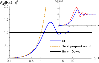
Figure 1: Power spectrum for a primordial SLE and window function (5.30) with support in $[-0.3,0.5]/H$. The insert shows in red the comparison with a situation where the window function has support in the pre-inflationary period $[-0.3,0]/H$ only.

6.  Conclusions

The States of Low Energy (SLE) were introduced as Hadamard states [5] on generic Friedmann-Lemaître spacetimes with a physically appealing defining property. Here we showed that SLE have several bonus properties which make them mathematically and physically even more attractive. These bonus properties (a) – (e) have been listed in the introduction and need not be repeated here. Instead, we comment on some extensions and future directions.

As seen, the minimization over initial data results in an instructive alternative expression for the SLE solution solely in terms of the commutator function. A minimization over boundary data would likewise be relevant and occurs naturally when placing the basic wave equation into the setting of a regular Sturm-Liouville problem. Taking advantage of the literature on non-regular Sturm-Liouville problems might allow one to extend the SLE construction systematically to situations where the coefficient functions become singular within the interval considered. Covering the big bang singularity is of prime interest, but other singular points may be worthwhile treating as well, as the model from Section 5 illustrates.

The computation of the power spectrum requires access to the cross-over regime in the (time, momentum) plane. Ideally, one would be able to treat also the cross-over regime analytically by a suitable expansion. Physicswise one would want to treat fully realistic cosmic evolutions where a pre-inflationary SLE replaces the positive frequency Hankel functions [32, 34, 35] and to propagate the resulting primordial power spectrum to the actual CMB.

Finally, it would be desirable to have a streamlined proof of the Hadamard property directly for SLE and including the massless case. The adiabatic vacua are a time-honored conduit and should be replaceable by more directly controllable WKB results for the large momentum regime, see e.g. [17].

Acknowledgements: This research was supported by Pitt-PACC. R.B. also acknowledges support by the Andrew Mellon Predoctoral Fellowship from the University of Pittsburgh.

References

- [1] I. Khavkine and V. Moretti, Algebraic QFT in curves spacetimes and quasifree Hadamard states: an introduction, in Advances in Algebraic QFT, R. Brunetti et al (eds), Springer, 2015.
- [2] C. Dappiaggi, V. Moretti, and N. Pinamonti, Hadamard States from Lightlike Hypersurfaces, Springer, 2017.
- [3] L. Parker and D. Toms, Quantum field theory in curved spacetime, Cambridge UP, 2009.
- [4] T. Hack, Cosmological applications of algebraic Quantum Field Theory in curved spacetimes, Springer, 2016.
- [5] H. Olbermann, States of low energy on Robertson-Walker spacetimes, Class. Quant. Grav. 24 (2007) 5011.
- [6] A. Degner and R. Verch, Cosmological particle creation in states of low energy, J. Math. Phys. 51 (2010) 022302.
- [7] K. Them and M. Brum, States of low energy in homogeneous and inhomogeneous expanding spacetimes, Class. Quant. Grav. 30 (2013) 23035.
- [8] C. Fewster and R. Verch, The necessity of the Hadamard condition, Class. Quant. Grav. 30 (2013) 235027.
- [9] S. Fulling, Remarks on positive energy and Hamiltonians in expanding Universes, Gen. Rel. Grav. 10 (1979) 807.
- [10] C. Lüders and J. Roberts, Local quasi-equivalence and adiabatic vacuum states, Commun. Math, Phys. 134 (1990) 29.
- [11] W. Junker and E. Schrohe, Adiabatic vacuum states on general spacetime manifolds: definition, construction, and physical properties, Ann. Henri Poincaré 3 (2002) 1113.
- [12] K. Pirk, Hadamard states and adiabatic vacua, Phys. Rev. D48 (1993) 3779.
- [13] N. Ashordi, S. Aslanbeigi, and R. Sorkin, A distingished vacuum state for a quantum field in a curved spacetimes: formalism, features, and cosmology, JHEP 2012 (2012) 1.
- [14] M. Brum and K. Fredenhagen, Vacuum-like Hadamard states for quantum fields on curved spacetimes, Class. Quant. Grav. 31 (2014) 025024.
- [15] L. Dickey, Soliton equations and Hamiltonian systems, World Scientific, 2003.
- [16] I. Avramidi, Heat kernel methods and its Applications, Birkhäuser, 2015.
- [17] G. Nemes, On the Borel summability of WKB solutions of certain Schrödinger-type differential equations, arXiv: 2004.13367.
- [18] M. Reed and B. Simon, Methods of Modern Mathematical Physics IV: Analysis of Operators, Academic Press/Elsevier 1978.
- [19] J. Guven, B. Lieberman, and C. Hill, Schrödinger picture field theory in Robertson-Walker flat spacetimes, Phys. Rev. D39 (1989) 438.
- [20] D. Long and G. Shore, The Schrödinger wave functional and vacuum states in curved spacetime I, II, Nucl. Phys. B530 (1998) 247, 279.
- [21] J. Koksma, T. Prokopec, and G. Rigopoulos, The scalar field kernel in cosmological spaces, Class. Quant. Grav 25 (2008) 125009.
- [22] L. Ford and L. Parker, Infrared divergences in a class of Robertson-Walker universes, Phys. Rev. D16 (1977) 245.
- [23] A. Higushi and N. Rendell, Infrared divergences for free quantum fields in cosmological spacetimes, Class. Quant. Grav. 35 (2018) 115004.
- [24] M. Fröb, T. Hack, and A. Higuchi, Compactly supported linearized observables in single field inflation, JCAP 07 (2017) 043.
- [25] J. Swieca, Goldstone’s theorem and related topics, in: Cargese lectures, 1969, Vol 4.
- [26] J. Lopuszanski, An introduction to symmetry and supersymmetry in quantum field theory, World Scientific, 1991.
- [27] S. Weinberg, Cosmology, Oxford UP, 2008.
- [28] J. Senovilla and D. Garfinkle, The 1965 Penrose singularity theorem, Class. Quant. Grav. 32 (2015) 124008.
- [29] S. Foster, Scalar field cosmology and the initial spacetime singularity, Class. Quant. Grav. 15 (1998) 3485.
- [30] W. Handley, S. Brechet, A. Lasenby, and M. Hobson, Kinetic initial conditions for inflation, Phys. Rev. D89 (2014) 063505.
- [31] C. Contaldi, M. Peleso, L. Kovman, and A. Linde, Suppressing the lower multipoles in the CMB anisotropies, Astropart. Phys. 07 (2003) 2.
- [32] B. Powell and W. Kinney, Pre-inflationary vacuum in the cosmic microwave background, Phys. Rev. D76 (2007) 063512.
- [33] T. Janssen and T. Prokopec, Regulating the infrared by mode-matching: a massless scalar in expanding spaces with constant deceleration, Phys. Rev. D83 (2011) 084035.
- [34] S. Das, G. Goswami, J. Prasad, and R. Rangarajan, Revisting a pre-inflationary radiation era and its effect on the CMB power spectrum, JCAP 06 (2015) 001.
- [35] G. Marozzi, M. Rinaldi, and R. Durrer, On infrared and ultraviolet divergences of cosmological perturbations, Phys. Rev. D83 (2011) 105017.