Predicting Livelihood Indicators from Community-Generated Street-Level Imagery

Abstract

Major decisions from governments and other large organizations rely on measurements of the populace’s well-being, but making such measurements at a broad scale is expensive and thus infrequent in much of the developing world. We propose an inexpensive, scalable, and interpretable approach to predict key livelihood indicators from public crowd-sourced street-level imagery. Such imagery can be cheaply collected and more frequently updated compared to traditional surveying methods, while containing plausibly relevant information for a range of livelihood indicators. We propose two approaches to learn from the street-level imagery: (1) a method that creates multi-household cluster representations by detecting informative objects and (2) a graph-based approach that captures the relationships between images. By visualizing what features are important to a model and how they are used, we can help end-user organizations understand the models and offer an alternate approach for index estimation that uses cheaply obtained roadway features. By comparing our results against ground data collected in nationally-representative household surveys, we demonstrate the performance of our approach in accurately predicting indicators of poverty, population, and health and its scalability by testing in two different countries, India and Kenya. Our code is available at https://github.com/sustainlab-group/mapillarygcn.

Introduction

In 2015, all member states of the United Nations adopted 17 Sustainable Development Goals , including eliminating poverty, achieving good health, and stimulating economic growth by 2030. To evaluate countries’ progress toward these goals, national governments and international organizations conduct nationally-representative household surveys that collect information on a range of livelihood indicators from households distributed throughout a given country. These surveys, such as the Demographic and Health Surveys (DHS) Program, provide critical insight into local economic and health conditions . However, they are costly and time-consuming, particularly when surveying remote populations linked by poor infrastructure. As a result, surveys are conducted infrequently or may only capture an extremely small proportion of households (Yeh et al. 2020). Satellite images and machine learning have been proposed as an alternative (Ayush et al. 2020b, a; Uzkent, Yeh, and Ermon 2020; Uzkent et al. 2019; Jean et al. 2016), but high-resolution imagery is expensive and obscures details of the ground level.

We introduce a scalable, interpretable approach that uses street-level imagery for livelihood prediction at a local level. We utilize Mapillary, a global citizen-driven street-level imagery database (Neuhold et al. 2017). Although Mapillary cannot match the consistent quality of commercial imagery, its widespread and growing availability in developing regions make it an appealing candidate as a passively collected data source for predicting livelihood indicators. In eight months, the Mapillary dataset doubled in size from 500 million images to 1 billion, with users capturing and verifying imagery from mobile devices .

We show how to capture information from Mapillary imagery to accurately predict livelihood indicators in India and Kenya, some of the most populous and economically diverse countries in the world. We present two complementary approaches: (1) The first creates representations for multi-household clusters by segmenting street-level images and aggregating informative objects, trains models, and interprets them using the most predictive features. (2) While the strength of the first approach is interpretability, we also propose a second to learn the relationships between images and leverage the inherent spatial structure of clusters by representing them as graphs, where each image is a feature-rich node connected by edges based on spatial distance.

Our approaches predict three indicators — poverty, population, and women’s body mass index (BMI, a key nutritional indicator) — in villages and urban neighborhoods. They achieve high classification accuracy and strong $r^{2}$ scores for regression in India and Kenya. Our method is a cheap, scalable, and effective alternative to traditional surveying to measure the well-being of developing regions.

Related Works

Recent research has explored the usage of passively collected data sources as cheaper alternatives to door-to-door or paper forms of data collection, to augment or eventually replace expensive household surveys. Proposed sources include social media (Signorini, Segre, and Polgreen 2011; Pulse 2014), mobile phone networks (Blumenstock, Cadamuro, and On 2015), Wikipedia (Sheehan et al. 2019), remote sensing, and street-level images.

Remote Sensing Data

Remote-sensing imagery from satellite or aircraft has been used to predict road quality in Kenya (Cadamuro, Muhebwa, and Taneja 2019), land use patterns in European cities (Albert, Kaur, and Gonzalez 2017), and economic outcomes in Africa and India (Jean et al. 2016; Yeh et al. 2020; Pandey, Agarwal, and Krishnan 2018; Ayush et al. 2020a). However, these approaches face challenges, such as poor generalizability to other locations or indicators (Head et al. 2017; Bruederle and Hodler 2018) and lack of nuance as local scenes are not visible from space. Street-level imagery provides greater detail (e.g. people) and local information.

Street-level Imagery

Past studies have used street-level imagery to measure social or health outcomes, but the focus has been in urban areas, predicting perceived safety of American cities with Google StreetView (Fu, Chen, and Lu 2018; Naik et al. 2014), analyzing urban perception from Baidu Maps or Tencent Maps in Chinese cities (Gong et al. 2019; Yao et al. 2019), identifying urban areas from human ratings of StreetView images in India (Galdo, Li, and Rama 2019), or predicting crime (Andersson et al. 2017) and voting patterns (Gebru et al. 2017) in U.S. cities. Our goal is to create approaches for developing regions that lack infrastructure by leveraging a community-generated data source, with an additional challenge that crowdsourced data can be noisy and inconsistent.

Another study that utilizes street-level imagery is (Suel et al. 2019), which trains a CNN to predict the best and worst-off deciles for outcomes like crime and self-reported health (it performs poorly for predicting objective health). The authors trained the CNN on Google StreetView imagery from London and demonstrated that learning could transfer to three other cities of the UK (Suel et al. 2019). We try the same method in our experiments, training a CNN on Mapillary images. However, given the noisy quality of the dataset and more difficult task of predicting accurately throughout developing countries and not just within developed cities, we require more sophisticated approaches to make improvements. For example, our graph convolutional network learns from multiple images, representing the spatial structure between them in edges, and encodes useful semantic features in the nodes. Furthermore, the visual makeup of cities in the same country can be similar, and it is a harder task for models to generalize to other countries. By performing experiments in India and Kenya, which have different data distributions, we show our approach can scale across countries.

Lastly, there are works that use crowdsourced imagery, i.e. Flickr, to predict the ambiance of London neighborhoods (Redi et al. 2018) and ”geo-attributes” such as GDP for gridded cells across the world (Lee, Zhang, and Crandall 2015). The latter is the most similar work since authors use a crowdsourced dataset to make predictions at a global, not solely urban, level. However, only 5% of Flickr’s imagery is geotagged (Hauff 2013). We found Mapillary is a more apt dataset for our work given its coverage of developing areas, exponential growth (Solem 2019), and geotagged imagery.

Datasets

First, we define the general problem of making predictions on geospatially located clusters. Assume there are $N$ geographic clusters. A cluster $i$ represents a circular area with center $c_{i}=(lat_{i},lon_{i})$. There is a set of street-level images that fall within its spatial boundaries, $\mathcal{X}_{i}=\{x_{i}^{0},x_{i}^{1},...,x_{i}^{n_{i}}\}$, where each $x_{i}^{j}\in\mathcal{X}$ is an image and $n_{i}$ is the total number of images. Each cluster also has $K$ surveyed variables of livelihood indicators, represented by $y_{i}$.

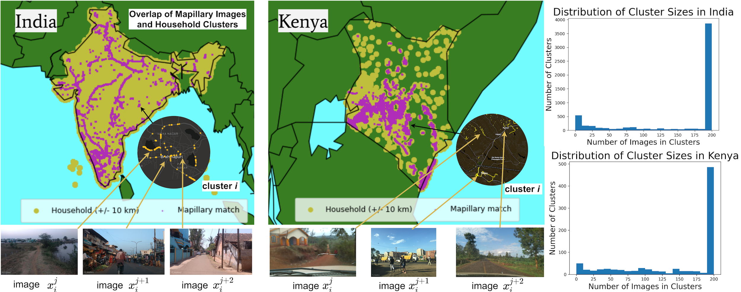
Figure 1: Left: Overlap of Mapillary images with household clusters for India and Kenya. Each map also contains a close-up view of a cluster $i$, where yellow dots represent its images. Right: Distribution of number of images per cluster in either country.

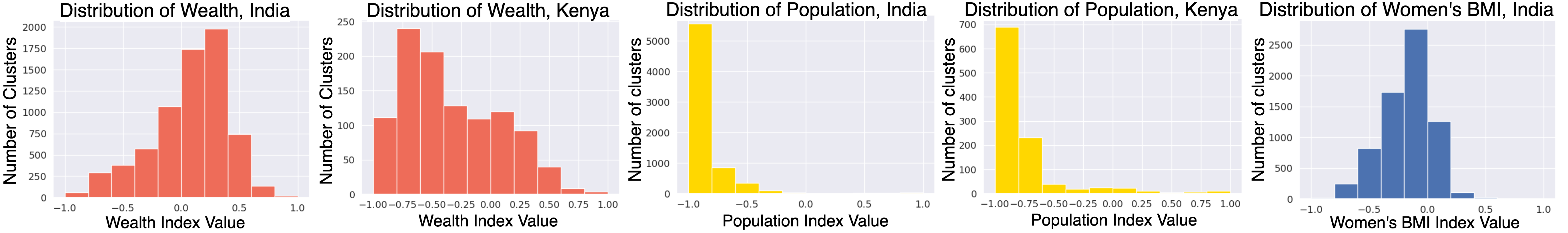
Figure 2: Left to right: Distributions of wealth (poverty is defined as its inverse) and population over India and Kenya. Distribution of women’s BMI in India. Note that binary labels are generated from a median split, so classes are balanced.

We aim to learn a mapping: $\mathcal{P}(\mathcal{X})\mapsto\mathcal{Y}$ to predict $y_{i}$ given $\mathcal{X}_{i}$, where $\mathcal{P}(\mathcal{X})$ is the powerset of $\mathcal{X}$ and $\mathcal{X}_{i}\in\mathcal{P}(\mathcal{X})$. The regression task entails predicting the indicator directly. Classification involves predicting a binary label, where an indicator value $\geq$ to the median results in a label of 1 and 0 otherwise. We perform these tasks over image sets $\mathcal{X}_{i}\in\mathcal{P}(\mathcal{X})$ as clusters have a variable number of images.

We specialize the general problem to a dataset of street-level imagery and cluster-level labels of indicators in India and Kenya. Each cluster represents a group of households within a 5km-radius area with label $y_{i}$, which contains the index value and class label for $K$ indicators. In India, $K=3$, i.e. poverty, population, and women’s BMI. In Kenya, $K=2$ as women’s BMI was not available. We discuss the data sources of $\mathcal{X}$ and $\mathcal{Y}$ in the following section.

Mapillary for Street-Level Images

The Mapillary API provides access to geo-tagged images and metadata. The data is community-driven, and anyone can create an account and upload images with EXIF embedded GPS coordinates or identify the location on a map. We matched images to household clusters, and only clusters with $n_{i}>0$ were kept. This resulted in 7,117 clusters and 1,121,444 images from India and 1,071 clusters and 156,756 images from Kenya. 98% of Mapillary images were available in high-resolution ($2048\times 1536$ px) and the remaining 2% in lower resolution ($640\times 420$ px).

Livelihood Indicators

We predict three varied livelihood indicators: poverty and population in both countries and a health-related measure in India. Each index is naturally continuous. The values are rescaled to be between -1 and 1 and used directly for regression. We split by the median to produce class labels. Figure 1 shows the overlap of Mapillary images and indicator labels, and Figure 2 shows the index distribution by country.

Poverty

We obtained wealth index values from the most recently completed surveys of the Demographic and Health Survey (DHS), 2015-16 for India and 2014 for Kenya. DHS data is clustered; households within a 5km-radius contribute datapoints individually but share the same geographic coordinates to preserve privacy. The index is calculated from assets and characteristics, such as vehicles, home construction material, etc. We consider poverty as the inverse of wealth.

Population

Facebook’s High Resolution Population Density Maps consist of geo-located population density labels across the world. Their data is much denser than that of Mapillary Vistas, so we average the values within a 5km radius of a cluster’s coordinate to produce its label.

Women’s BMI

Women’s body-mass-index (BMI) is an important indicator of human well-being. We compute BMI by dividing weight in kilograms by height in meters squared for the 697,486 samples in the DHS survey and average the values across all women in a cluster to produce its label.

Methods

Given this dataset constructed with geotagged Mapillary images and indexes, we propose methods to learn the mapping $\mathcal{P}(\mathcal{X})\mapsto\mathcal{Y}$. We focus on two learning paradigms: (1) image-wise learning where a model learns from a single image, $x_{j}\in\mathcal{X}_{i}$, sampled from cluster $c_{i}$, and (2) cluster-wise learning where a model learns from all images $\mathcal{X}_{i}$ in $c_{i}$.

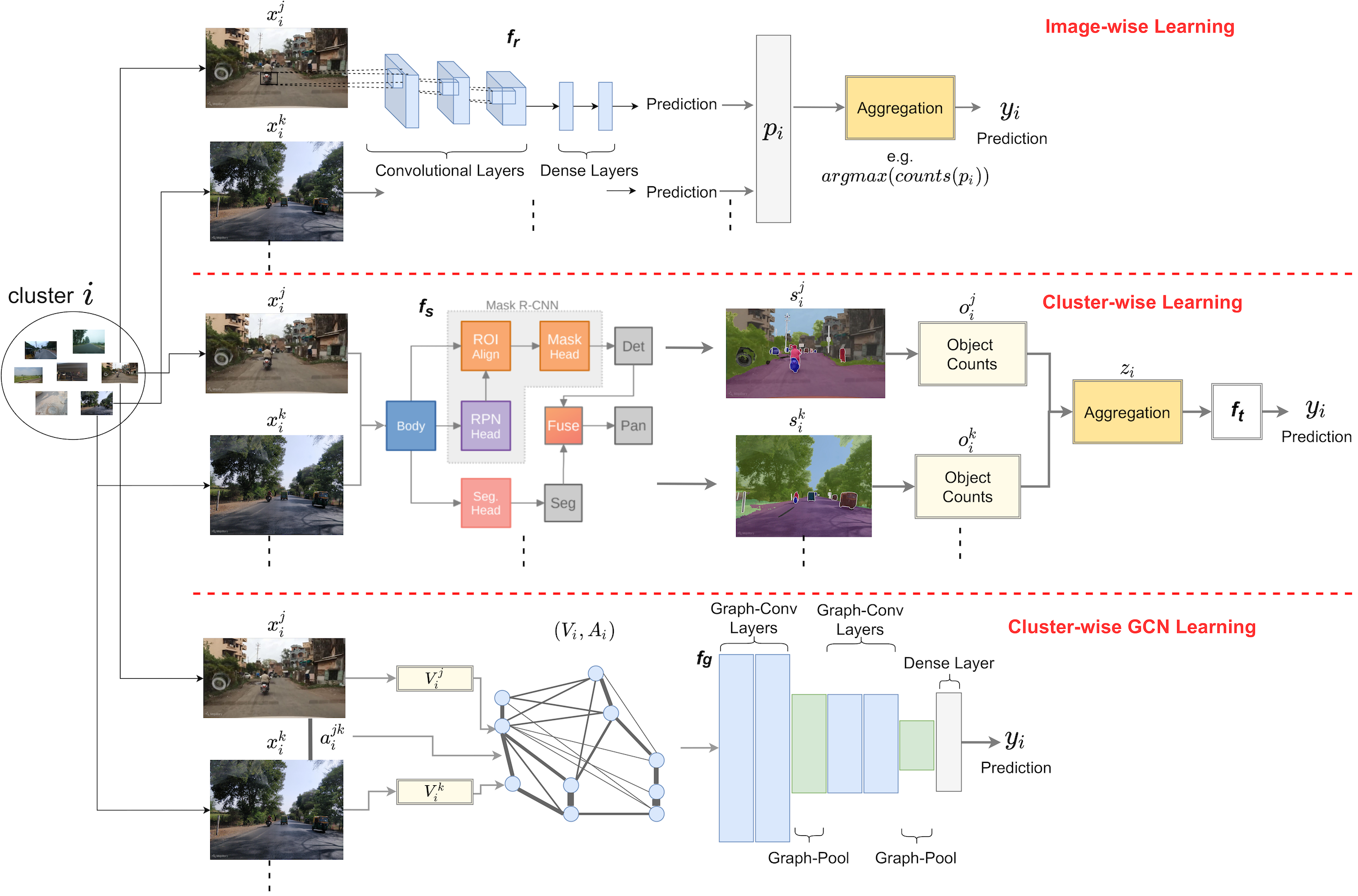
Figure 3: Overview of the proposed methods. Top: image-wise learning, which learns mapping $f_{r}$ from imagery as in (Suel et al. 2019). Middle: cluster-wise learning, which uses a panoptic segmentation model to create cluster-level representations and learns the mapping $f_{t}$. Bottom: GCN that represents clusters as a fully connected set of images. Some connections are left out in the above figure for the sake of clarity. Using Graph-Conv layers followed by a Graph-Pool layer, it learns mapping $f_{g}$.

Image-wise Learning

As did (Suel et al. 2019), we directly map each individual image in the cluster, $x_{j}\in\mathcal{X}_{i}$, to the label space. We refer to the model that learns this mapping as ResNet-ImageWise. As in Figure 3, image-wise predictions, $p_{i}$, are combined at test time using an aggregation strategy to produce final predictions, $y_{i}$. Each prediction is considered a vote, and the majority class is considered the final prediction for cluster $i$.

Cluster-wise Learning

Learning from Cluster Level Object Counts

In this section, we propose a method to utilize object counts from street-level images in a cluster. Image level object counts are aggregated across the cluster to create cluster-wise object counts. Finally, we train a classifier or regression model on cluster-level object counts to predict indexes.

Panoptic Segmentation on Mapillary Images

With the Mapillary Vistas (Neuhold et al. 2017) panoptic segmentation dataset, we can train a network to segment street-level images. Mapillary Vistas has 28 stuff and 37 thing classes, where stuff refers to amorphous regions, i.e. ”nature,” and things are enumerable objects, i.e. ”car.” It contains 25,000 annotated images with an average resolution of $\sim$9 megapixels captured at various conditions, times, and viewpoints (e.g. from a windshield, while walking, etc.), making Mapillary Vistas an ideal dataset to train a segmentation model.

We use the seamless scene segmentation model proposed by (Porzi et al. 2019). The model consists of two main modules–instance segmentation and semantic segmentation–and the third module fuses predictions from both to generate panoptic segmentation masks. The instance segmentation module uses Mask-RCNN (He et al. 2017), and the semantic segmentation module uses an encoder-decoder architecture similar to the Feature Pyramid Network (Lin et al. 2017). Finally, ResNet50 is used to parameterize the backbone model. During training, the Mapillary images are scaled such that the shortest size is $1024\times t$ pixels, where $t$ is randomly sampled from the interval $[0.5,2.0]$. The authors report $50.4\%$ mean IoU (intersection over union) score on the Mapillary Vistas test set. To be consistent with the trained model, we scale our Mapillary images such that the shortest size is represented by 1024 px.

Cluster Level Object Counts

Using the seamless scene segmentation model, we segment every image $x_{i}^{j}\in X_{i}$ in a cluster with the hypothesis that the 65 different roadway features provide useful information. The authors of (Ayush et al. 2020b) correlated object detections from satellite imagery with poverty in Uganda and used them as interpretable features. We expected to discover patterns as well, such as more bike racks appearing in high-wealth areas. Each image $x_{i}^{j}\in\mathcal{X}_{i}$ maps to a set of object detections $o_{i}^{j}$, where $o_{i}^{j}\in\mathbb{R}^{65}$. We then sum the number of instances for each class, or $\sum_{j=0}^{n_{i}}o_{i}^{j}$. To avoid bias towards clusters with many images, we append a feature with the total number of images in a cluster, or $n_{i}$. Each cluster is represented by a feature vector $z_{i}\in\mathbb{R}^{66}$. We map these interpretable embeddings to the label space and refer to the models as Obj-ClusterWise.

Graph Convolutional Networks

The methods thus far process images independently. We propose Graph Convolutional Networks (GCN) (Such et al. 2017) to learn relationships between images, representing a cluster as a graph, where image-based features serve as nodes connected by edges encoding their spatial distance. Each graph has a matrix $\mathcal{V}$ for nodes and $\mathcal{A}$ for edges. Our task is to learn the mapping: $f_{g}$: ($\mathcal{V}_{i}$, $\mathcal{A}_{i}$) $\mapsto$ $y_{i}$. We refer to these models as GCN. Since we model image connections with scalars, the GCN uses a convex combination of the adjacency and identity matrix to create a filter $\mathcal{H}$ that convolves $\mathcal{V}$ before passing the output through a ReLU activation and Dropout (Graph-Conv). Graph Embed Pooling (Graph-Pool) is the corollary for MaxPooling and treats the Graph-Conv output as an embedding matrix, reducing $\mathcal{V}$ and $\mathcal{A}$ to a desired number of vertices.

Node Representations

Each image in a cluster is represented by a node, which is composed of CNN features from ResNet-ImageWise, detected object counts ($o_{i}^{j}$ in Obj-ClusterWise), or the combination of the two. The node representations for any cluster $i$ is $\mathcal{V}_{i}\in\mathbb{R}^{n_{i}\times d}$, where $n_{i}$ is the maximum number of images per cluster and $d$ is the size of feature vector for each image.

Modeling Connections Between Nodes

There is an inherent spatial structure to clusters as Mapillary images uploaded by users are geo-tagged and captured while driving or walking on roads. We take advantage of this structure by connecting the image nodes. We initialize $\mathcal{A}$ as the normalized inverse distance between two images in a cluster. That is, let $d_{i}^{jk}=distance(x_{i}^{j},x_{i}^{k})$ be the spatial distance in kilometer unit between two images $x_{i}^{j}$ and $x_{i}^{k}$ in cluster $i$. Let the maximum distance between any two images in any one cluster is $d_{max}$. In this case, for $a_{i}^{jk}\in\mathcal{A}_{i}$, $a_{i}^{jk}=1-\frac{d_{i}^{jk}}{d_{max}}$. This way, we construct matrix $\mathcal{A}$ using a scalar for each edge and we get: $\mathcal{A}_{i}\in\mathcal{R}^{n_{i}}$ for any cluster $i$.

Experiments

			Wealth		Population		BMI
Eval Region	Feature	Method	Acc.	$r^{2}$	Acc.	$r^{2}$	Acc.	$r^{2}$
India	Image	ResNet-ImageWise (Suel et al. 2019)	74.34	0.51	93.50	0.85	85.28	0.52
India	Object Counts	MLP (3-layer)	74.98	0.52	91.71	0.81	82.60	0.53
India	Object Counts	Random Forest	75.77	0.52	88.99	0.79	83.49	0.54
India	Object Counts	GBDT	74.91	0.51	89.35	0.78	83.63	0.52
India	Object Counts	kNN (k=3)	68.69	0.34	85.78	0.75	77.98	0.36
India	Object Counts	GCN	72.05	0.39	86.63	0.86	80.13	0.38
India	CNN Embeddings	GCN	81.06	0.54	94.71	0.82	89.42	0.57
India	CNN Embeddings + Object Counts	GCN	80.91	0.53	94.42	0.89	89.56	0.56
India	Object Counts	Random Forest 50% Pooled	74.20	0.45	86.49	0.67	N/A
India	CNN Embeddings + Object Counts	GCN 50% Pooled	80.99	0.52	94.07	0.81
India	Object Counts	Random Forest 100% Pooled	74.98	0.52	89.78	0.76
India	CNN Embeddings + Object Counts	GCN 100% Pooled	81.34	0.51	94.50	0.88
Kenya	Image	ResNet-ImageWise (Suel et al. 2019)	73.71	0.39	87.79	0.90	N/A
Kenya	Object Counts	MLP (3-layer)	77.34	0.43	89.59	0.81
Kenya	Object Counts	Random Forest	75.59	0.50	86.38	0.81
Kenya	Object Counts	GBDT	72.77	0.50	86.38	0.81
Kenya	Object Counts	kNN (k=3)	70.42	0.38	82.63	0.53
Kenya	Object Counts	GCN	71.36	0.35	88.26	0.80
Kenya	CNN Embeddings	GCN	76.06	0.42	89.67	0.84
Kenya	CNN Embeddings + Object Counts	GCN	75.59	0.40	89.67	0.85
Kenya	Object Counts	Random Forest 50% Pooled	74.18	0.41	81.69	0.51	N/A
Kenya	CNN Embeddings + Object Counts	GCN 50% Pooled	76.53	0.38	89.20	0.79
Kenya	Object Counts	Random Forest 100% Pooled	74.18	0.47	86.85	0.58
Kenya	CNN Embeddings + Object Counts	GCN 100% Pooled	77.00	0.36	90.14	0.72
Avg of Both	None (Baseline)	Random	50.70	-	50.11	-	51.47	-
Avg of Both	Lat/Lon Coords (Baseline)	Avg of Neighbors	63.57	0.16	69.06	0.66	66.17	0.25

Table 1: Results on predicting wealth, population, and BMI. The method in (Suel et al. 2019) serves as an additional baseline. To the best of our knowledge, we are the first to present a scalable, intereptable pipeline to make predictions from only crowdsourced street-level imagery across India and Kenya.

We perform extensive experiments on our dataset consisting of Mapillary images and ground-truth indexes. As our work is the first to utilize Mapillary for indicator prediction, we build baselines to benchmark our model performance. The metrics are classification accuracy and the square of the Pearson correlation coefficient (Pearson’s $r^{2}$) for regression. For each country, we randomly sample 80% of the clusters as the training set and the remainder is the validation set.

Baselines

For each cluster, we predict a local (geographic) average of neighboring clusters as a baseline. This simulates how we often have access to district-level statistics about livelihood indicators. We approximate the district-level values as the mode or mean (in the case of binary classification and regression, respectively) of the 1,000 clusters closest to $c_{i}$. In other words, the baseline predicts the $\hat{y}$ from $\mathcal{Y}_{i}^{sort}\subseteq\mathcal{Y}$, where $\mathcal{Y}_{i}^{sort}$ represents a subset of clusters sorted by distance to $c_{i}$ in increasing order where $|\mathcal{Y}_{sort}|=1000$.

Implementation Details

For ResNet-ImageWise, all images $\mathcal{X}$ are resized to $224\times 224\times 3$. We train a ResNet34 (He et al. 2016) model initialized with weights pretrained on ImageNet (Russakovsky et al. 2015) to learn a mapping $f_{r}$ from image to $y_{i}\in\mathbb{R}^{K}$. There is one classification and one regression label for each indicator ($K=6$). We train with batch size 128 and learning rate 0.001 (after trying 0.1, 0.01, and 0.0001) for 50 epochs on a NVIDIA 1080TI GPU with 40G of memory.

We train different models as part of Obj-ClusterWise, which map the object counts feature to the label space. For the classification task, we use a 3-layer Multi-Layer Perceptron (layer size 256, ReLU activation, learning rate of 0.001), Random Forest (300 trees), Gradient Boosted Decision Trees (300 boosting stages), and k-Nearest Neighbors ($k=3$). The same models are used for regression.

For the GCN, we feed the representation of image nodes via $\mathcal{V}$ and node connections via $\mathcal{A}$ into two Graph-Conv layers of size 64 (each followed by a ReLU activation) followed by a Graph-Pool of size 32. Then there is another pair of Graph-Conv layers of size 32 and a Graph-Pool of size 8. The resulting output is then fed into a fully connected dense layer of size 256 and a final output layer of size 2 for binary classification or size 1 for regression. We trained with a batch size of 256 and learning rate of 0.0001 on a NVIDIA 1080TI GPU. We use Adam optimizer (Kingma and Ba 2014) for all the experiments in this study.
Pooled Models for Transferability We also train models that pool data from both India and Kenya to assess whether learning transfers. We train a Obj-ClusterWise model and a GCN model in two experimental settings. In the first, we randomly sample 50% of clusters from the training datasets of both countries, train the model, and evaluate on India and Kenya separately (50% Pooled). In the second setting, the models learn from all training clusters from both countries and evaluate on India and Kenya separately (100% Pooled).

Predictions on Livelihood Indicators

Poverty

ResNet-ImageWise, which is the baseline method from (Suel et al. 2019), achieves 74.34% accuracy in India and 73.71% in Kenya. Models that use cluster-wise representations perform better than the baselines. Obj-ClusterWise leverages the semantic information of object counts, obtaining 75.77% in India and 77.34% in Kenya. The GCN makes further improvements, achieving 81.06% in India, learning from both the visual features and spatial relationships between images. The 100% Pooled GCN achieves the best accuracy in India. As in Figure 2, Kenya is more left-skewed than India in its wealth distribution, providing additional examples of low-wealth clusters. For regression, wealth does not persist over large areas and can shift between clusters, so the baseline does especially poorly. Obj-ClusterWise methods achieved $r^{2}$ scores of 0.52 to 0.54 in India and the best score of 0.50 in Kenya, suggesting the semantic information encoded by object counts is useful.

Population

The GCN attained 94.71% accuracy in India and 89.67% accuracy in Kenya. The 100% Pooled GCN achieved the best performance in Kenya at 90.14%. The GCN also obtained the highest $r^{2}$, 0.89, in India. We hypothesized there would be clear visual indicators of population captured by imagery and detections (e.g. instances of ”person,” infrastructure, or transportation), which may explain why the GCN that uses both image embeddings and object counts performs strongly (further explored in next section).

Women’s BMI

BMI is a health-related indicator that may not be obvious from imagery, but one that our models learn to predict effectively. BMI data was not available for Kenya in the 2014 DHS, so we report results in India. The GCN achieved 89.56% classification accuracy and 0.57 $r^{2}$. Neither high nor low BMI is desirable, so for future experiments we plan to classify a healthy BMI, between 18.5 to 24.9 .

We observe the method from (Suel et al. 2019) is not adequate and make significant improvements on most tasks by leveraging cluster-wise representations. The GCN, which is designed to learn relationships between images through feature-rich nodes and spatial distance-based edges, attains the best performance on most tasks. Obj-ClusterWise models perform comparably, relying only on object counts, suggesting they capture useful semantic information. Pooled models achieve the best or close to best performance for most tasks, so learning a combination of spatial information, object counts, and visual features can be useful to generalize across countries, which will be useful for practitioners.

Analysis: Effect of Number of Images

We analyzed how many images are necessary for a cluster to be sufficiently representative. We took random samples of images, from 50 to 200 (the maximum size), from each cluster. We then trained an MLP model for 100 epochs with a learning rate of 1e-3 and evaluated it on classification in each country. As shown in Figure 4, more images led to increased accuracy, but surprisingly a relatively small number of images, even 50, was enough to achieve good accuracy.

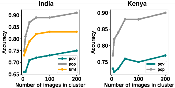
Figure 4: Accuracy vs. # of images per cluster.

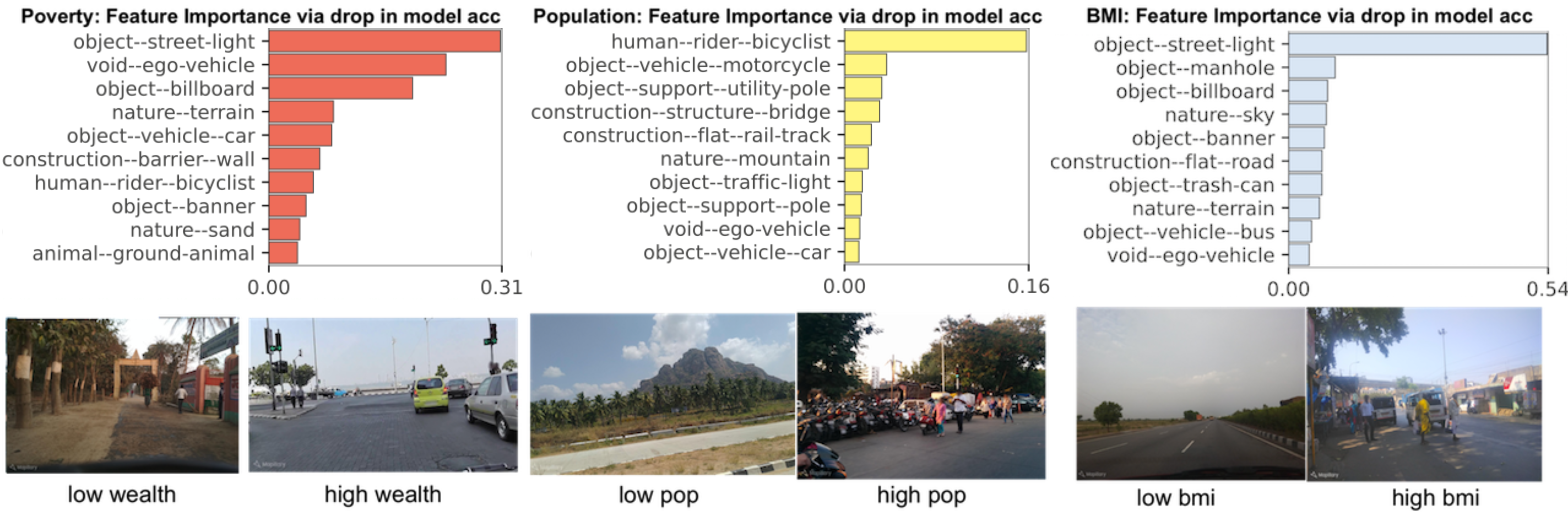
Figure 5: Top: Feature importance by indicator. We train a pooled random forest model, using data from both countries, for poverty and population. Women’s BMI data was not available in Kenya, so the BMI features are India-specific. We use permutation importance because it is more reliable than mean-decrease-in-impurity importance (Strobl et al. 2007), which can be highly biased when predictors variables vary in their scale of measurement or number of categories, as in our case.

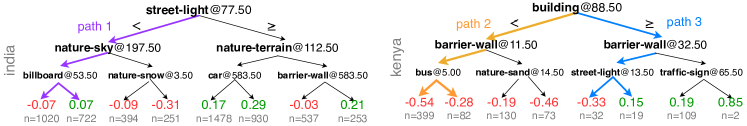
Figure 6: Decision tree visualizations. A decision tree classifier is trained for poverty regression in each country and then visualized . Each node displays the object class and threshold that determines how to split the node (left child means $<$ the threshold, right child $\geq$ the threshold). Visualizations for all indicators in Supplementary Material.

Interpretability using Object Counts

Interpretability of the predictions is an important aspect to consider for estimates from machine learning models to be adopted by policymakers and practitioners (Ayush et al. 2020b; Murdoch et al. 2019). Currently, the DHS constructs a wealth index using principal component analysis (PCA) on hand-collected characteristics of households, such as assets (i.e. televisions, bicycles, etc.), materials for housing construction, and types of water access . We demonstrate how models can learn from features visible from the road, offering a much cheaper but still effective method of index estimation. Moreover, many existing models trained from passively collected data sources (Jean et al. 2016; Cadamuro, Muhebwa, and Taneja 2019; Sheehan et al. 2019) are accurate but not inherently interpretable. We examine which objects are important for a given index and visualize decision trees to help end-user organizations understand the model. Although the GCN model performs strongly, CNN features are difficult to interpret compared to semantic objects. The 100% Pooled Random Forest model performs closely with only object counts, so we use this model for interpretation.

Feature Importance

As shown in Figure 5, signs of development, i.e. vehicles, traffic lights, street lights, and construction, were important in poverty prediction. Instances of terrain (e.g. dirt or exposed ground alongside a road) were also informative, likely because they suggest a lack of urbanization. For population, infrastructure, i.e. rail tracks and bridges, and transportation modes, i.e. bicyclist, motorcycle, and truck, were important. For women’s BMI, the most salient features were streetlights, manholes, and billboards, indicating the presence of services and development.

Visualizing Decision Trees

We train decision tree regressors with a max depth of 3 to predict poverty and then visualize them (Figure 7). At each node, moving left means the cluster has fewer than the threshold number of objects (right means $\geq$ to the threshold). Final predictions are at the leaves, where $n$ is the number of clusters with that prediction. We demonstrate how to use the trees by tracing paths:
Path 1: As expected, a cluster with few street lights is predicted as low-wealth, shown by how most leaves have negative values. Billboards, representing storefronts and ads, are also informative, with fewer leading to a negative estimate.
Path 2: Few buildings and barrier walls leads to a low-wealth prediction. These construction-type barrier walls are salient (used in the second level of the tree), indicating sites of development and growth for organizations to monitor.
Path 3: Alternatively, many buildings but few barrier walls signal varying levels of development. Street lights become important, as more instances correlate with higher estimates.

Conclusion

In this work, we present a novel approach to make predictions on poverty, population, and women’s body-mass index from street-level imagery. In spite of the inconsistent quality of such a large-scale, crowd-sourced dataset, we achieve strong performance in predicting indicators that have not previously been the focus of machine learning methods, such as women’s BMI, a key nutritional indicator. We demonstrate how our method is scalable, making predictions across India and Kenya. We present two approaches: (1) cluster-wise learning, which represents household clusters from detected object counts and enables interpretability and (2) a graph-based approach that aims to capture the spatial structure of a cluster, representing images as feature-rich nodes connected by edges based on spatial distance. We hope that our method can be employed as a cheap but effective alternative to traditional surveying methods for organizations to measure the well-being of developing regions.

References

- Albert, Kaur, and Gonzalez (2017) Albert, A.; Kaur, J.; and Gonzalez, M. C. 2017. Using Convolutional Networks and Satellite Imagery to Identify Patterns in Urban Environments at a Large Scale. In Proceedings of the 23rd ACM SIGKDD International Conference on Knowledge Discovery and Data Mining, KDD ’17, 1357–1366. New York, NY, USA: Association for Computing Machinery. ISBN 9781450348874. doi:10.1145/3097983.3098070. URL https://doi.org/10.1145/3097983.3098070.
- Andersson et al. (2017) Andersson, V. O.; Birck, M. A. F.; Araujo, R. M.; and Cechinel, C. 2017. Towards Crime Rate Prediction through Street-level Images and Siamese Convolutional Neural Networks. In ENIAC - Encontro Nacional de Inteligência Artificial e Computacional.
- Ayush et al. (2020a) Ayush, K.; Uzkent, B.; Burke, M.; Lobell, D.; and Ermon, S. 2020a. Efficient Poverty Mapping using Deep Reinforcement Learning. arXiv preprint arXiv:2006.04224 .
- Ayush et al. (2020b) Ayush, K.; Uzkent, B.; Burke, M.; Lobell, D.; and Ermon, S. 2020b. Generating Interpretable Poverty Maps using Object Detection in Satellite Images.
- Blumenstock, Cadamuro, and On (2015) Blumenstock, J.; Cadamuro, G.; and On, R. 2015. Predicting poverty and wealth from mobile phone metadata. Science 350(6264): 1073–1076.
- Bruederle and Hodler (2018) Bruederle, A.; and Hodler, R. 2018. Nighttime lights as a proxy for human development at the local level. PloS one 13(9): e0202231.
- Cadamuro, Muhebwa, and Taneja (2019) Cadamuro, G.; Muhebwa, A.; and Taneja, J. 2019. Street smarts: measuring intercity road quality using deep learning on satellite imagery. In Proceedings of the 2nd ACM SIGCAS Conference on Computing and Sustainable Societies, 145–154.
- Fu, Chen, and Lu (2018) Fu, K.; Chen, Z.; and Lu, C.-T. 2018. StreetNet: Preference Learning with Convolutional Neural Network on Urban Crime Perception. In Proceedings of the 26th ACM SIGSPATIAL International Conference on Advances in Geographic Information Systems, SIGSPATIAL ’18, 269–278. New York, NY, USA: Association for Computing Machinery. ISBN 9781450358897. doi:10.1145/3274895.3274975. URL https://doi.org/10.1145/3274895.3274975.
- Galdo, Li, and Rama (2019) Galdo, V.; Li, Y.; and Rama, M. 2019. Identifying urban areas by combining human judgment and machine learning: An application to India. Journal of Urban Economics 103229. ISSN 0094-1190. doi:https://doi.org/10.1016/j.jue.2019.103229. URL https://www.sciencedirect.com/science/article/pii/S0094119019301068.
- Gebru et al. (2017) Gebru, T.; Krause, J.; Wang, Y.; Chen, D.; Deng, J.; Aiden, E. L.; and Fei-Fei, L. 2017. Using deep learning and Google Street View to estimate the demographic makeup of neighborhoods across the United States. Proceedings of the National Academy of Sciences 114(50): 13108–13113. ISSN 0027-8424. doi:10.1073/pnas.1700035114. URL https://www.pnas.org/content/114/50/13108.
- Gong et al. (2019) Gong, Z.; Ma, Q.; Kan, C.; and Qi, Q. 2019. Classifying Street Spaces with Street View Images for a Spatial Indicator of Urban Functions. Sustainability 11: 6424. doi:10.3390/su11226424.
- Hauff (2013) Hauff, C. 2013. A study on the accuracy of Flickr’s geotag data. In Proceedings of the 36th International ACM SIGIR Conference on Research and Development in Information Retrieval, SIGIR ’13, 1037–1040. doi:10.1145/2484028.2484154.
- He et al. (2017) He, K.; Gkioxari, G.; Dollár, P.; and Girshick, R. 2017. Mask r-cnn. In Proceedings of the IEEE international conference on computer vision, 2961–2969.
- He et al. (2016) He, K.; Zhang, X.; Ren, S.; and Sun, J. 2016. Deep Residual Learning for Image Recognition. In 2016 IEEE Conference on Computer Vision and Pattern Recognition (CVPR), 770–778. doi:10.1109/CVPR.2016.90.
- Head et al. (2017) Head, A.; Manguin, M.; Tran, N.; and Blumenstock, J. E. 2017. Can human development be measured with satellite imagery? In ICTD.
- Jean et al. (2016) Jean, N.; Burke, M.; Xie, M.; Davis, W. M.; Lobell, D. B.; and Ermon, S. 2016. Combining satellite imagery and machine learning to predict poverty. Science 353(6301): 790–794. ISSN 0036-8075. doi:10.1126/science.aaf7894. URL https://science.sciencemag.org/content/353/6301/790.
- Kingma and Ba (2014) Kingma, D. P.; and Ba, J. 2014. Adam: A method for stochastic optimization. arXiv preprint arXiv:1412.6980 .
- Lee, Zhang, and Crandall (2015) Lee, S.; Zhang, H.; and Crandall, D. J. 2015. Predicting geo-informative attributes in large-scale image collections using convolutional neural networks. In 2015 IEEE Winter Conference on Applications of Computer Vision, 550–557. IEEE.
- Lin et al. (2017) Lin, T.-Y.; Dollár, P.; Girshick, R.; He, K.; Hariharan, B.; and Belongie, S. 2017. Feature pyramid networks for object detection. In Proceedings of the IEEE conference on computer vision and pattern recognition, 2117–2125.
- Murdoch et al. (2019) Murdoch, W. J.; Singh, C.; Kumbier, K.; Abbasi-Asl, R.; and Yu, B. 2019. Definitions, methods, and applications in interpretable machine learning. Proceedings of the National Academy of Sciences 116(44): 22071–22080. ISSN 0027-8424. doi:10.1073/pnas.1900654116. URL https://www.pnas.org/content/116/44/22071.
- Naik et al. (2014) Naik, N.; Philipoom, J.; Raskar, R.; and Hidalgo, C. 2014. Streetscore – Predicting the Perceived Safety of One Million Streetscapes. In 2014 IEEE Conference on Computer Vision and Pattern Recognition Workshops, 793–799.
- Neuhold et al. (2017) Neuhold, G.; Ollmann, T.; Rota Bulò, S.; and Kontschieder, P. 2017. The Mapillary Vistas Dataset for Semantic Understanding of Street Scenes. In International Conference on Computer Vision (ICCV). URL https://www.mapillary.com/dataset/vistas.
- Pandey, Agarwal, and Krishnan (2018) Pandey, S.; Agarwal, T.; and Krishnan, N. C. 2018. AAAI Conference on Artificial Intelligence. In Multi-Task Deep Learning for Predicting Poverty From Satellite Images. URL https://www.aaai.org/ocs/index.php/AAAI/AAAI18/paper/view/16441.
- Porzi et al. (2019) Porzi, L.; Bulo, S. R.; Colovic, A.; and Kontschieder, P. 2019. Seamless Scene Segmentation. In The IEEE Conference on Computer Vision and Pattern Recognition (CVPR).
- Pulse (2014) Pulse, U. G. 2014. Mining Indonesian Tweets to understand food price crises. Jakarta: UN Global Pulse .
- Redi et al. (2018) Redi, M.; Aiello, L. M.; Schifanella, R.; and Quercia, D. 2018. The Spirit of the City: Using Social Media to Capture Neighborhood Ambiance. Proc. ACM Hum.-Comput. Interact. 2(CSCW). doi:10.1145/3274413. URL https://doi.org/10.1145/3274413.
- Russakovsky et al. (2015) Russakovsky, O.; Deng, J.; Su, H.; Krause, J.; Satheesh, S.; Ma, S.; Huang, Z.; Karpathy, A.; Khosla, A.; Bernstein, M.; et al. 2015. Imagenet large scale visual recognition challenge. International journal of computer vision 115(3): 211–252.
- Sheehan et al. (2019) Sheehan, E.; Meng, C.; Tan, M.; Uzkent, B.; Jean, N.; Lobell, D.; Burke, M.; and Ermon, S. 2019. Predicting Economic Development using Geolocated Wikipedia Articles. arXiv preprint arXiv:1905.01627 .
- Signorini, Segre, and Polgreen (2011) Signorini, A.; Segre, A. M.; and Polgreen, P. M. 2011. The use of Twitter to track levels of disease activity and public concern in the US during the influenza A H1N1 pandemic. PloS one 6(5): e19467.
- Solem (2019) Solem, J. E. 2019. A Look Back at 2019 and the Road to One Billion Images. URL https://blog.mapillary.com/update/2019/12/16/the-road-to-one-billion-images.html. Last Accessed: Feb 2nd, 2020.
- Strobl et al. (2007) Strobl, C.; Boulesteix, A.-L.; Zeileis, A.; and Hothorn, T. 2007. Bias in random forest variable importance measures: Illustrations, sources and a solution. BMC Bioinformatics 8(1): 25. ISSN 1471-2105. doi:10.1186/1471-2105-8-25. URL https://doi.org/10.1186/1471-2105-8-25.
- Such et al. (2017) Such, F. P.; Sah, S.; Domínguez, M.; Pillai, S.; Zhang, C.; Michael, A.; Cahill, N. D.; and Ptucha, R. W. 2017. Robust Spatial Filtering with Graph Convolutional Neural Networks. CoRR abs/1703.00792. URL http://arxiv.org/abs/1703.00792.
- Suel et al. (2019) Suel, E.; Polak, J. W.; Bennett, J. E.; and Ezzati, M. 2019. Measuring social, environmental and health inequalities using deep learning and street imagery. Scientific Reports 9(1): 6229. ISSN 2045-2322. doi:10.1038/s41598-019-42036-w. URL https://doi.org/10.1038/s41598-019-42036-w.
- Uzkent et al. (2019) Uzkent, B.; Sheehan, E.; Meng, C.; Tang, Z.; Burke, M.; Lobell, D.; and Ermon, S. 2019. Learning to interpret satellite images in global scale using wikipedia. arXiv preprint arXiv:1905.02506 .
- Uzkent, Yeh, and Ermon (2020) Uzkent, B.; Yeh, C.; and Ermon, S. 2020. Efficient object detection in large images using deep reinforcement learning. In The IEEE Winter Conference on Applications of Computer Vision, 1824–1833.
- Yao et al. (2019) Yao, Y.; Liang, Z.; Yuan, Z.; Liu, P.; Bie, Y.; Zhang, J.; Wang, R.; Wang, J.; and Guan, Q. 2019. A human-machine adversarial scoring framework for urban perception assessment using street-view images. International Journal of Geographical Information Science 33(12): 2363–2384. doi:10.1080/13658816.2019.1643024. URL https://doi.org/10.1080/13658816.2019.1643024.
- Yeh et al. (2020) Yeh, C.; Perez, A.; Driscoll, A.; Azzari, G.; Tang, Z.; Lobell, D.; Ermon, S.; and Burke, M. 2020. Using publicly available satellite imagery and deep learning to understand economic well-being in Africa. Nature Communications 11(1): 1–11.