Visibility Guided NMS: Efficient Boosting of Amodal Object Detection in Crowded Traffic Scenes

Abstract

Object detection is an important task in environment perception for autonomous driving. Modern 2D object detection frameworks such as Yolo, SSD or Faster R-CNN predict multiple bounding boxes per object that are refined using Non-Maximum Suppression (NMS) to suppress all but one bounding box. While object detection itself is fully end-to-end learnable and does not require any manual parameter selection, standard NMS is parametrized by an overlap threshold that has to be chosen by hand. In practice, this often leads to an inability of standard NMS strategies to distinguish different objects in crowded scenes in the presence of high mutual occlusion, e.g. for parked cars or crowds of pedestians. Our novel Visibility Guided NMS (vg-NMS) leverages both pixel-based as well as amodal object detection paradigms and improves the detection performance especially for highly occluded objects with little computational overhead. We evaluate vg-NMS using KITTI, VIPER as well as the Synscapes dataset and show that it outperforms current state-of-the-art NMS.

1 Introduction

Object detection is the task of drawing a tight bounding box around an object of interest in an image while still covering all parts of this object. There are two possible ways to perform object detection: one option is to predict the pixel-based box which is restricted to only those parts of an object that are visible in the image. The other possibility is to predict a box covering the entire object – even if it is not fully visible in the image, for example due to partial occlusion by other objects. Humans perceive the environment in the latter way, an ability called amodal perception, which enables enhanced reasoning about a scene as it carries additional information on the geometry and full spatial extent of a given object. Figure 1 illustrates the difference between these two paradigms.

Independent of which object detection paradigm is chosen, the majority of the modern object detectors – such as Yolo [34, 32, 33], SSD [28, 11] or Faster-RCNN [15, 35] – are built upon CNN architectures and follow a three-step scheme during inference: (i) a set of initial bounding boxes – known as prior boxes or anchor boxes – are spread over the whole image. These template boxes are (ii) refined to match the outline of the object that is to be detected. Finally, all detections are (iii) processed to remove duplicates using Non-Maximum Suppression (NMS) [16, 15, 28, 32]. While today’s object detection frameworks are fully end-to-end trainable for steps (i) and (ii), NMS in its commonly used way is still a non-learnable algorithm that requires manual parameter tuning. Due to its simplicity, standard NMS is extremly fast while still yielding reasonable results for many applications.

NMS ranks all detections by their score and iteratively removes all candidates that exceed a manually chosen Intersection-over-Union (IoU) threshold, usually between 0.3 and 0.5. Detections with a smaller overlap are accepted as valid bounding boxes. However, as shown in Figure 2, there often exist many objects whose respective bounding boxes overlap more strongly than this carefully chosen threshold, but which are valid nonetheless and would falsely be suppressed. This behaviour can lead to problems e.g. in crowded traffic scenarios as by design some objects can never be detected, even if the network predicted them correctly.

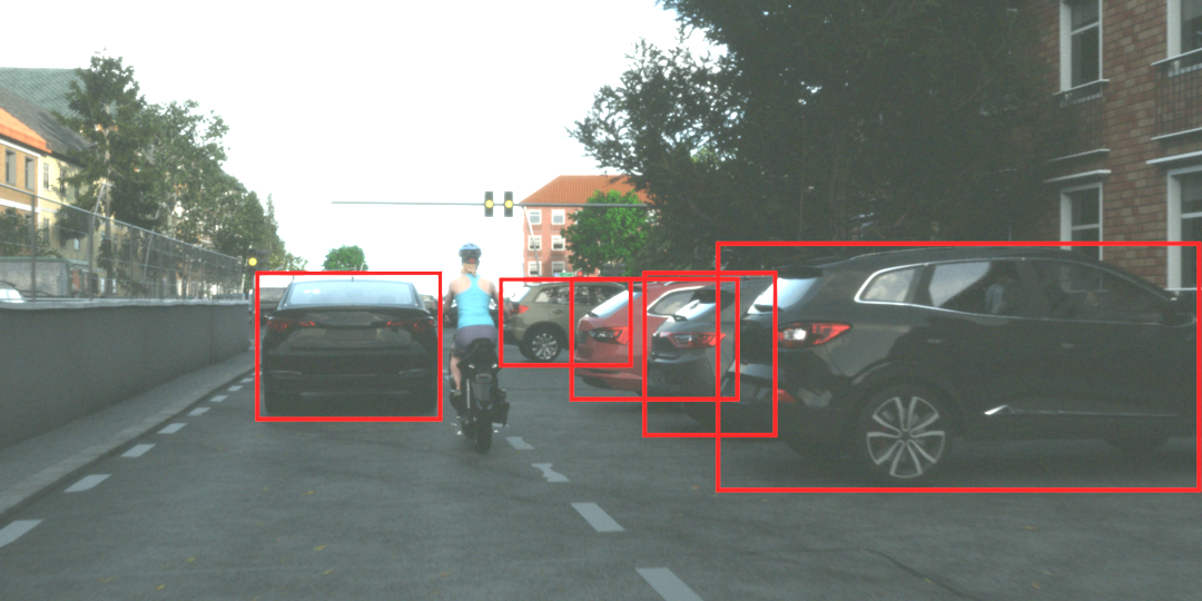
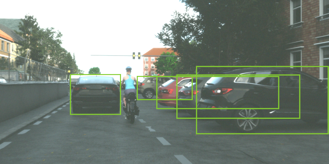
Figure 1: Left: Pixel-based bounding boxes. These bounding boxes only surround visible parts in the image. Right: Amodal bounding boxes. The full extend of the vehicles is surrounded by the bounding box providing a richer representation of the object. Image taken from the Synscapes dataset [42].

One solution to this problem is to predict pixel-based bounding boxes, as they tend to have lower bounding box overlap for mutually occluded objects than their amodal counterparts. However, this induces a loss of information as the full spatial extent of the object is no longer considered.

Our goal is to improve amodal object detection and its relatively poor detection performance. We summarize our contributions as follows: (i) We propose a novel NMS variant that we call Visibility Guided NMS (vg-NMS). For vg-NMS only little computational overhead is required as it is built upon joint pixel-based and amodal object detection. In contrast to other approaches no additional subnetworks are required. (ii) Due to its simple and efficient design, vg-NMS can be included in any object detector that features standard NMS. (iii) We evaluate vg-NMS on different and challenging datasets tailored especially for autonomous driving and show that it outperforms standard NMS and its variants.

2 Related Work

While amodal perception is a well addressed problem in instance segmentation [25, 45, 10, 9] only little attention is paid to amodal object detection in 2D. However, even instance segmentation can benefit from amodal object detection e.g. when using Mask R-CNN [17] as an amodal instance segmentation framework.

For pure object detection Deng and Latecki [8] show the potential of successfully lifting amodal 2D object detections to 3D space in an indoor setting using the NYU v2 dataset [7] using RGB-D data.

Especially in an autonomous driving context, several approaches make use of amodal object detection. The authors of [29, 12, 13, 41] use monocular RGB images to detect 3D vehicles and estimate their orientation. To this end these approaches feature an amodal object detection framework and the final 2D detections are enriched with additional 3D information. Gählert et al. [12, 13] build on specific keypoints in 2D that – given the camera projection matrix – allow for 3D estimates. All approaches are evaluated on the KITTI Object Detection and Orientation Estimation benchmark [14]. However, most of these methods use 2D object detectors that feature standard NMS which tends to perform poorly on amodal bounding boxes compared to pixel-based ones as shown in Figure 2.

There are several approaches addressing NMS related issues. Soft NMS [2] ranks candidates by their scores after re-weighting them depending on their IoU overlap with close-by predictions. He et al. [18, 19] propose a novel bounding box regression loss that improves detection performance in combination with a variant of Soft NMS called Softer NMS. Fitness NMS [40] include a fitness coefficient that measures the IoU overlap between the prediction and any GT bounding box.

Liu et al. [27] improve pedestrian detection performances in a crowd by estimating the object density in the image and applying dynamic object suppression during NMS. To this end, an additional density estimator subnet is required.

Another approach of overcoming issues induced by NMS is to model NMS as a fully end-to-end learnable part within the actual object detection framework. Hosang et al. [20, 21] convert the NMS scheme into an additional CNN-subnet, finally making NMS learnable.

However, appending additional networks like Hosang et al. [21] and Liu et al. [27] results in longer inference time which reduces their merit for fully autonomous driving where compute is limited and realtime capable algorithms are crucial. Hence, we focus on optimizing NMS with as little computational overhead as possible to allow for productive in-vehicle use. Contrary to Liu et al. [27], we do not only focus on pedestrians and extend detection to Cars/Vans and Trucks/Buses.

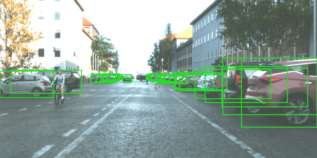
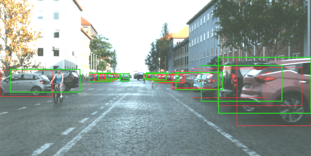
Figure 2: Left: Amodal GT data. Right: If standard NMS is applied on the GT data, several boxes (red) will be removed leading to a bad detection performance. Image taken from the Synscapes dataset [42].

3 Joint Pixel-Based and Amodal Object Detection

To allow for simultaneous amodal and pixel-based object detection several straight forward adjustments are required in the network as well as the loss design.

We explain the modifications exemplarily for the Single Shot Multibox Detector (SSD) [28] framework, a one-stage detector that performs object classification as well as bounding box regression in one step.

SSD features a CNN backbone network and places multiple prior boxes – template bounding boxes of different sizes and aspect ratios – that are placed regularly all over the image. During training, these prior boxes are trained to match the outlines of the object of interest. During inference for each box the class probabilities $p_{i}$ as well as the adjustments relative to the prior box $\delta_{x},\delta_{y},\delta_{w},\delta_{h}$ will be predicted. For each prior box there are $4+(n_{c}+1)$ free parameters with $n_{c}$ being the number of different classes. The numbers of prior boxes vary depending on the image size. E.g. for KITTI there are approx. $11,000$ prior boxes in our setting while VIPER with a resolution of $1920\text{\times}1080\text{\,}\mathrm{px}$ already has nearly $50,000$ prior boxes.

3.1 Adjustments in Object Detection Framework

Architecture:

To combine pixel-based and amodal object detection, slight adjustments in the network architecture are required. As each prior box is now asked to predict two bounding boxes, we add 4 additional regression parameters to each prior box leading to $4+4+(n_{c}+1)$ free parameters per prior box. The first set of regression parameters is trained to predict the pixel-based bounding boxes while the second set focuses on the amodal bounding boxes.

Compared to the standard SSD setting, these adjustments therefore introduce only a slight overhead of $n\times 4$ parameters with $n$ being the number of priors per image.

During training, the matching between prior and ground truth boxes is solely done using the first set of regression parameters corresponding to the pixel-based bounding boxes.

Loss:

Usually object detection frameworks feature a classification and box regression i.e. localization loss

$$L_{\text{total}}=L_{\text{cls}}+\alpha L_{\text{loc}}$$ (1)

where $\alpha$ denotes a weighting factor between the two losses. Common localization losses are e.g. (Smooth) L1, L2, IoU or gIoU [36] loss. For classification tasks Cross-Entropy Loss (CE) or its improved version Focal Loss [26] are commonly used.

For joint detection two different objectives must be optimized for – i.e. the regression of pixel-based and amodal bounding boxes. The overall localization loss is thus composed of two terms:

$$L_{\text{loc}} =\beta L_{\text{loc,pix}}+\gamma L_{\text{loc,amodal}}.$$ (2)

Hence the total loss is given by

$$L_{\text{total}} =L_{\text{cls}}+\beta L_{\text{loc,pix}}+\gamma L_{\text{loc,amodal}}.$$ (3)

In our experiments we use $\alpha=1$ for networks that only perform one detection task. For joint pixel-based and amodal object detection we find $\beta=1$ and $\gamma=2$ to be a good combination.

3.2 Visibility Guided NMS

To ensure that both pixel-based as well as amodal prior boxes at index $i$ will cover the same physical object, we employ element-wise sharing of the classifier weights between both sets of prior boxes $\mathcal{P}_{\text{pix}}$ and $\mathcal{P}_{\text{amodal}}$. An object covered by the corresponding prior boxes will therefore yield the same classification result.

The main idea of Visibility Guided NMS (vg-NMS) is to perform NMS on the pixel-based bounding boxes that describe the actually visible parts of the object, but output the amodal bounding boxes that belong to the indices that are retained during pixel-based NMS. For a set of initial detections $\mathcal{B}$, standard NMS returns a set of indices $\mathcal{I}$ containing all indices of detections in $\mathcal{B}$ that are retained during the NMS. Finally the corresponding boxes in $\mathcal{B}$ are selected by indices $\mathcal{I}$ yielding the final set of detections $\mathcal{D}$.

In contrast, vg-NMS combines standard NMS with the two different sets of object predictions $\mathcal{B}_{\text{pix}}$ and $\mathcal{B}_{\text{amodal}}$ and performs standard NMS on $\mathcal{B}_{\text{pix}}$ returning a set of indices $\mathcal{I}_{\text{pix}}$. The final valid detections both for pixel-based $\mathcal{D}_{\text{pix}}$ and amodal bounding boxes $\mathcal{D}_{\text{amodal}}$ are chosen by $\mathcal{I}_{\text{pix}}$.

Figure 3: vg-NMS compared to standard NMS for an amodal object detection task for a crowded traffic scene with many heavily overlapping objects. While standard NMS removes too many boxes, vg-NMS keeps bounding boxes for each object despite their huge overlap.

Figure 3 and algorithm 1 illustrate vg-NMS both visually and as pseudocode.

1

2VisibilityGuidedNMS $(\mathcal{B}_{\text{pix}},\mathcal{B}_{\text{amodal}})$;

Input : Set of predictions $\mathcal{B}_{\text{pix}}$, $\mathcal{B}_{\text{amodal}}$

Output : Set of detections $\mathcal{D}_{\text{pix}}$, $\mathcal{D}_{\text{amodal}}$

3

4$\mathcal{I}_{\text{pix}}\leftarrow$ NMS$(\mathcal{B}_{\text{pix}})$;

5 $\mathcal{D}_{\text{pix}}\leftarrow$ select$(\mathcal{B}_{\text{pix}},\mathcal{I}_{\text{pix}})$;

$\mathcal{D}_{\text{amodal}}\leftarrow$ select$(\mathcal{B}_{\text{amodal}},{\color[rgb]{1,0,0}\mathcal{I}_{\text{pix}}})$ ;

  /* $\mathcal{I}_{\text{pix}}$ is used here */

return $\mathcal{D}_{\text{pix}}$, $\mathcal{D}_{\text{amodal}}$

Algorithm 1 vg-NMS.

4 Experiments

4.1 Datasets and Evaluation Metrics

Several datasets exist that are tailored specifically for autonomous driving purposes. However, most of the datasets focus on specific tasks such as semantic and instance segmentation or object detection. An overview of currently available datasets is shown in Table 1. Only few datasets feature amodal object detection and even less datasets feature both amodal and pixel-based object detection. Fortunately, if instance segmentation data is available, pixel-based bounding boxes can easily be generated.

For our experiments we select KITTI [14], Viper [37] and Synscapes [42] as these datasets contain annotations for both amodal as well as pixel-based bounding boxes. KITTI contains nearly $15,000$ real images with a resolution of approx. $380\text{\times}1250\text{\,}\mathrm{px}$. Synscapes ($720\text{\times}1440\text{\,}\mathrm{px}$) and VIPER ($1080\text{\times}1920\text{\,}\mathrm{px}$) are synthetic datasets with outstanding and nearly photorealistic graphics. Synscapes contains $25,000$ images and VIPER, the most exhaustive resource of the three, offers more than $250,000$ images.

For KITTI we follow [43] to create a train-val-split. This ensures that no images from the same sequence are seen during both training and validation. Please note that KITTI does not provide official semantic and instance segmentation data. Instead we use KINS [31], which extends KITTI with the corresponding labels. Unfortunately, the label definitions used for KINS are not in full concordance with the definitions used in the original KITTI dataset.

VIPER offers an official train-val-split. For Synscapes, we selected the first $80\text{\,}\mathrm{\char 37\relax}$ of the $25,000$ images as a training set and hold out the remaining $20\text{\,}\mathrm{\char 37\relax}$ for validation. All experiments were evaluated on the respective validation sets.

As all datasets follow different labeling strategies we select three shared classes with matching definitions accross all datasets: (i) cars & vans, (ii) trucks & buses and (iii) pedestrians. Motorbikes and bicycles are not labeled in all datasets, hence we do not consider these objects to allow for a valid comparison.

While for Synscapes and VIPER there is no official object detection benchmark available, KITTI provides such a benchmark. However, as the label definitions as used within our experiments do not match the exact definitions for this benchmark, we did not evaluate on the official KITTI benchmark.

Table 1: Current datasets tailed especially for autonomous driving. For object detection not all datasets feature both pixel-based as well amodal bounding boxes.

		Annotations
Name	Real	Pixel-based 2D Box	Amodal 2D Box	3D Box
KITTI [14]	✓	✓ (KINS [31])	✓	✓
Cityscapes [6]	✓	✓	✗	✗
BDD100k [44]	✓	✓	✗	✗
ApolloScape [22]	✓	✓	✗	✓ (Lidar)
Mapillary [30]	✓	✓	✗	✗
Nuscenes [3]	✓	✗	✓	✓
Lyft [23]	✓	✗	✓	✓
Waymo Open Dataset [1]	✓	✗	✓	✓
Synthia [38]	✗	✓	✓	✓
VIPER [37]	✗	✓	✓	✓
Synscapes [42]	✗	✓	✓	✓

As shown in Figure 2 in a standard NMS setting, all objects with an overlap greater than a specific threshold – e.g. $0.45$ – cannot be resolved. However, especially for vehicles there is a higher fraction of objects with high overlap in amodal object bounding boxes compared to pixel-based bounding boxes. By using vg-NMS the non-resolvable objects will decrease to the pixel-based fraction and thus will yield better results.

For each dataset we train a network specialized for the task of detecting amodal bounding boxes and compare these with a network that features joint pixel-based and amodal object detection and vg-NMS.

We use Mean Average Precision (mAP) as the evaluation metric and exclude all boxes with a size of smaller than $20\text{\times}20\text{\,}\mathrm{px}$ as detecting small objects is a challenging task for all object detectors [4]. Other benchmarks use similar exclusion criteria, e.g. KITTI excludes all boxes with a size of smaller than $25\text{\times}25\text{\,}\mathrm{px}$. In Cityscapes [6] all objects with a size of less than $10\text{\times}10\text{\,}\mathrm{px}$ are not taken into account during evaluation. Additionally, IoU calculation is very unstable for very small objects leading to a higher number of False Positives (FP) as well as False Negatives (FN).

Other evaluation methods like KITTI [14] also ignore heavily occluded or truncated boxes. As vg-NMS specifically addresses this scenario, we do not exclude these boxes to allow for a realistic assessment of its performance. Furthermore, we require an IoU overlap of $0.5$ to accept a detection as a True Positive (TP).

4.2 Theoretical Problem Analysis

Each dataset is evaluated to quantify the theoretically possible improvement for detection performance for both pedestrians as well as vehicles including cars, vans, trucks and buses.

As standard NMS removes objects instead of spawning new ones, the number of False Negatives (FN) will increase yielding a decreased Recall value $R=\tfrac{TP}{TP+FN}$. The maximal theoretically possible Recall values are shown in Table 2 and an in-depth analysis is given in the appendix A.1.

Table 2: Theoretically improvements of vg-NMS. The maximum possible Recall values $R_{\text{max}}$ and $R_{\text{vg}}$ are given for the standard NMS as well as the vg-NMS. Furthermore the number of objects per image is given. We only consider boxes with a size of at least $20\text{\times}20\text{\,}\mathrm{px}$ as smaller objects are hard to identify even for humans. Especially for vehicles there is huge potential of theoretical improvments by using vg-NMS.

	Vehicles				Pedestrians
	$R_{\text{max}}$	$R_{\text{vg}}$	$\Delta$ [%]	#/image	$R_{\text{max}}$	$R_{\text{vg}}$	$\Delta$ [%]	#/image
KITTI [14]	$0.956$	$0.965$	+$0.94$	$2.9$	$0.978$	$0.982$	+$0.41$	$0.4$
VIPER [37]	$0.948$	$0.981$	+$3.48$	$3.7$	$0.951$	$0.980$	+$3.05$	1.4
Synscapes [42]	$0.869$	$0.939$	+$8.05$	$7.1$	$0.918$	$0.952$	+$3.75$	$7.9$

While KITTI is the only dataset used in this study that features real-world data, it is the dataset with the smallest possible improvements compared to VIPER and Synscapes. This is because KITTI includes only a few valid objects per image compared to VIPER and Synscapes since it includes traffic scenes from both urban and overland environments. The latter scenario of course features crowded scenes much less frequently.

A more reasonable real-world dataset for the evaluation on crowded traffic scenes is Cityscapes [6] as it mainly focuses on urban environments. However, with an average of $4.2$ and $8.4$ bounding boxes per image for the pedestrian and vehicle class respectively, the typical scene composition in Cityscapes is similar to the Synscapes dataset, making it an adequate surrogate for our purposes.

Please note that these theoretical values can only be reached if the underlying object detector perfectly predicts all bounding boxes. In practice these numbers may therefore vary or $R_{\text{max}}$ as well as $R_{\text{vg}}$ might not be reached at all.

4.3 Results

Table 3: Average Precision (AP) results of different NMS variants for amodal object detection. Evaluation was performed on the validation splits of each dataset. vg-NMS outperforms both standard and Soft NMS and shows excellent performance in combination with Soft NMS.

		AP [%]
		Car / Van	Truck / Bus	Pedestrian	mAP	Runtime*
KITTI [14]	Standard NMS	$80.26$	$37.12$	$62.57$	$59.98$	$21.2\text{\,}\mathrm{ms}$
	Soft	$79.86$	$36.88$	$62.24$	$59.66$	$71.3\text{\,}\mathrm{ms}$
	vg	$80.65$	$36.46$	$63.74$	$60.29$	$22.8\text{\,}\mathrm{ms}$
	vg + Soft	$80.30$	$36.54$	$63.51$	$60.12$	$75.2\text{\,}\mathrm{ms}$
VIPER [37]	Standard NMS	$72.28$	$33.30$	$51.49$	$52.36$	$35.5\text{\,}\mathrm{ms}$
	Soft	$72.40$	$33.34$	$51.46$	$52.40$	$85.3\text{\,}\mathrm{ms}$
	vg	$72.98$	$33.47$	$54.78$	$53.74$	$37.4\text{\,}\mathrm{ms}$
	vg + Soft	$73.04$	$33.53$	$54.80$	$53.79$	$68.4\text{\,}\mathrm{ms}$
Synscapes [42]	Standard NMS	$83.97$	$84.62$	$87.33$	$85.31$	$26.7\text{\,}\mathrm{ms}$
	Soft	$83.66$	$84.59$	$86.99$	$85.08$	$113.1\text{\,}\mathrm{ms}$
	vg	$88.25$	$85.61$	$89.68$	$87.85$	$28.2\text{\,}\mathrm{ms}$
	vg + Soft	$88.26$	$85.63$	$89.60$	$87.83$	$78.8\text{\,}\mathrm{ms}$

* For Soft NMS we use TensorFlow’s built-in function non_max_suppression_v5 which is still under development and not yet publically available in an official release. We suspect that due to the implementation runtime of Soft NMS increases with the number of box predictions with high IoU overlap. In case of amodal object detection much more predictions have a high overlap, hence Soft NMS is much slower for amodal bounding boxes compared to pixel-based ones. E.g. for a subset of 100 Synscapes images we find in average $2.35$ times more amodal bounding boxes with an IoU overlap of more than $0.45$ compared to pixel-based bounding boxes.

All experiments were conducted under the same setup. We use TensorFlow and InceptionV1 [39] as a backbone for our SSD network. We trained the networks using the Adam optimizer [24] with a learning rate of $lr=0.0001$, $\beta_{1}=0.9$, $\beta_{2}=0.999$ and a batch size of 1. Every training was performed multiple times with different random seeds and evaluated after each epoch using the validation set. Finally, the results of the best snapshots are reported. During training we choose L2 as the bounding box regression loss $L_{\text{loc}}$ for both pixel-based and amodal bounding boxes. Furthermore, we use Focal Loss [26] as the classification task loss. Both training and inference were performed on an NVIDIA Titan RTX.

Table 3 shows the results for the standard NMS setting as well as for Soft NMS and vg-NMS. Qualitative results of vg-NMS are shown in the appendix A.2.

For all datasets vg-NMS outperforms standard NMS and Soft NMS. The combination of Soft and vg-NMS often yields even better results. Especially for VIPER and Synscapes the detection performance was significantly increased. This is in concordance to Table 2 where we expect the most gain in performance primarily for datasets with crowded scenes – i.e. many overlapping objects in one image.

While detection performance is improved, the runtime of vg-NMS remains comparable or even decreases: On average, vg-NMS is just $6.2\text{\,}\mathrm{\char 37\relax}$ slower when paired with a standard hard suppresion strategy. This amounts to less than $2\text{\,}\mathrm{ms}$ computational overhead due to the simultanous estimation of both pixel-based and amodal bounding boxes. Furthermore, vg-NMS is capable of significantly reducing the overall runtime if used in combination with Soft NMS for both VIPER and Synscapes images. We suspect that this is because pixel-based boxes inherently overlap less strongly with each other than their amodal counterparts. Hence the number of candidate pairings that need to be considered during the score reweighting step in Soft NMS is significantly smaller for pixel-based bounding boxes.

4.4 Ablation Study

By simultaneously predicting both pixel-based and amodal bounding boxes we de facto created a multitask setting as two tasks are optimized in parallel. Caruana [5] shows that multitask learning inherently improves the overall detection performance as it allows for better generalizations of the features that are learned.

Hence, we evaluate all 3 datasets regarding their performance in the single task networks and in the multitask setting. For these experiments we use the same data as for the previous ones. The results are shown in Table 4.

As expected, the simultaneous regression of both pixel-based and amodal object detection leads to an improved single task performance.

Table 4: Single task Average Precision (AP) results for standard NMS for both single task and multitask networks. Evaluation was performed on the validation splits of each dataset. Regressing both pixel-based and amodal bounding boxes jointly leads to an improvement compared the single task setting.

			AP [%]
	Box type	Network	Car / Van	Truck / Bus	Pedestrian	mAP
KITTI [14]	Pixel	Single	$78.37$	$36.89$	$63.18$	$59.51$
	Pixel	Multi	$79.24$	$36.25$	$62.71$	$59.40$
	Amodal	Single	$80.26$	$37.12$	$62.57$	$59.98$
	Amodal	Multi	$80.26$	$36.58$	$63.54$	$60.12$
VIPER [37]	Pixel	Single	$75.28$	$38.41$	$48.47$	$54.05$
	Pixel	Multi	$76.88$	$40.48$	$49.45$	$55.60$
	Amodal	Single	$72.28$	$33.30$	$51.49$	$52.36$
	Amodal	Multi	$72.39$	$33.25$	$55.32$	$53.65$
Synscapes [42]	Pixel	Single	$84.25$	$82.72$	$86.54$	$84.50$
	Pixel	Multi	$85.11$	$83.58$	$87.26$	$85.32$
	Amodal	Single	$83.97$	$84.62$	$87.33$	$85.31$
	Amodal	Multi	$85.41$	$85.84$	$88.76$	$86.67$

5 Conclusion

In this paper a new variant of Non-Maximum Suppression (NMS) called Visibility Guided NMS (vg-NMS) was proposed. vg-NMS can be used to boost amodal object detection in crowded traffic scenes as it prevents highly occluded amodal bounding boxes from being falsely suppressed. In contrast to other techniques we do not require an additional subnet but only need labeled GT data for both pixel-based as well as amodal bounding boxes. While vg-NMS itself does not need any additional computation, slight adjustments in the network design are required to allow for a simultaneous detection of both types of bounding boxes. In average these adjustments cause an increase of runtime of only $6.2\text{\,}\mathrm{\char 37\relax}$. Furthermore, we showed that simultaneous pixel-based and amodal bounding object detection also leads to an improved performance in the single task setting without vg-NMS.

vg-NMS can be included in all modern object detectors such as SSD [28], YOLO [32] or Faster RCNN [35]. We evaluated vg-NMS on KITTI, VIPER and Synscapes – datasets tailored especially for autonomous driving – and show that vg-NMS outperforms standard NMS as well as Soft NMS especially in crowded scenarios with a high number of objects per image.

Appendix A Appendix

A.1 In-Depth Theoretical Analysis

For each dataset we analyze the distribution of overlapping objects for all vehicles (including cars, trucks and buses) as well as for pedestrians. As bicycles and motorbikes are not labeled in each dataset, these vehicles are excluded in our analysis. For each image in the dataset we opt for the maximum IoU of one bounding box with any other object.

The corresponding histograms are shown in Figure 4 and zoomed to all IoU overlaps $>0.05$. All objects above the IoU threshold – in our experiments we set it to $0.45$ – cannot be resolved. Hence the number of False Negatives (FN) will increase. Given the appearance histogram with bins $i\in\mathcal{B}$ with density $p(i)$, IoU threshold $t_{\text{IoU}}$ we will find for the theoretical maximum True Positive (TP), False Negative (FN) and Recall ($R$) values for amodal object detection

$$TP_{\text{max}} =1-\sum_{i>t_{\text{IoU}}}^{1}p_{\text{amodal}}(i)$$ (4)

$$FN_{\text{max}} =\sum_{i>t_{\text{IoU}}}^{1}p_{\text{amodal}}(i)$$ (5)

$$R_{\text{max}} =\frac{TP_{\text{max}}}{TP_{\text{max}}+FN_{\text{max}}}$$ (6)

$$=1-\sum_{i>t_{\text{IoU}}}^{1}p_{\text{amodal}}(i).$$ (7)

For vg-NMS these theoretical upper bounds can be calculated as

$$TP_{\text{vg}} =1-\sum_{i>t_{\text{IoU}}}^{1}\underbrace{\left(p_{\text{amodal}}(i)-p_{\text{pix}}(i)\right)}_{\kappa_{i}}$$ (8)

$$FN_{\text{vg}} =\sum_{i>t_{\text{IoU}}}^{1}\underbrace{\left(p_{\text{amodal}}(i)-p_{\text{pix}}(i)\right)}_{\kappa_{i}}$$ (9)

$$R_{\text{vg}} =\frac{TP_{\text{vg}}}{TP_{\text{vg}}+FN_{\text{vg}}}$$ (10)

$$=1-\sum_{i>t_{\text{IoU}}}^{1}\left(p_{\text{amodal}}(i)-p_{\text{pix}}(i)\right)$$ (11)

$$=1-\sum_{i>t_{\text{IoU}}}^{1}p_{\text{amodal}}(i)+\sum_{i>t_{\text{IoU}}}^{1}p_{\text{pix}}(i)$$ (12)

$$R_{\text{vg}} =R_{\text{max}}+\sum_{i>t_{\text{IoU}}}^{1}p_{\text{pix}}(i).$$ (13)

As shown in Figure 4 the coefficient $\kappa_{i}$ is very small for pedestrians compared to vehicles. Hence, vehicles benefit the most of vg-NMS. An overview about the theoretical improvements is shown in Table 2.

Figure 4: Histograms for vehicles and pedestrians in the VIPER, KITTI and Synscapes dataset for both amodal and pixel-based bounding boxes. Due to the standard NMS design all detections with an IoU of greater than e.g. $0.45$ cannot be resolved. For amodal bounding boxes a higher number of objects will be lost due to NMS.

A.2 Visual Examples

The following images are taken from the val split of each dataset. For KITTI the images are part of the official test set.

A.2.1 KITTI

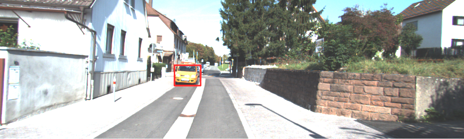
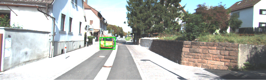
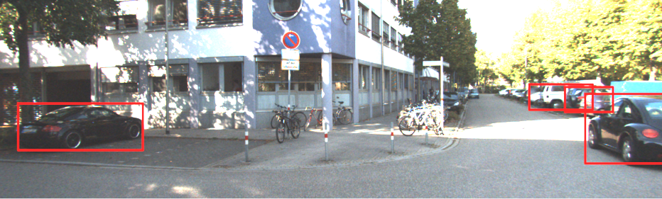
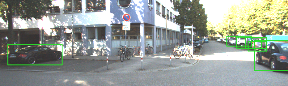
Figure 5: Left: Final detections without vg-NMS. Right: Final detections with vg-NMS.

A.2.2 VIPER

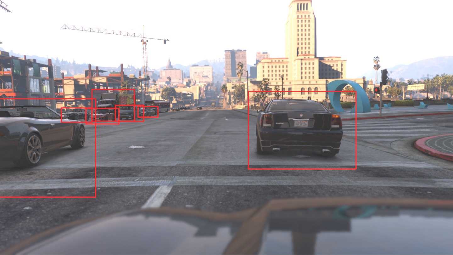
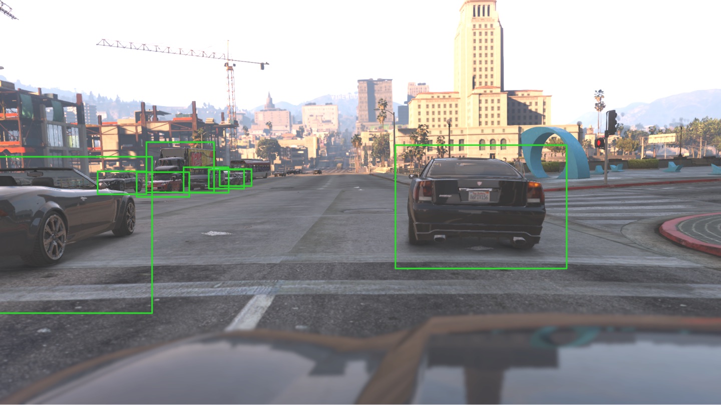
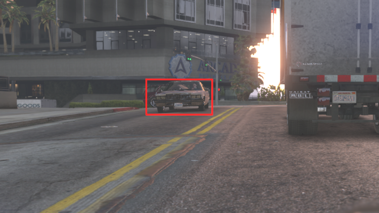
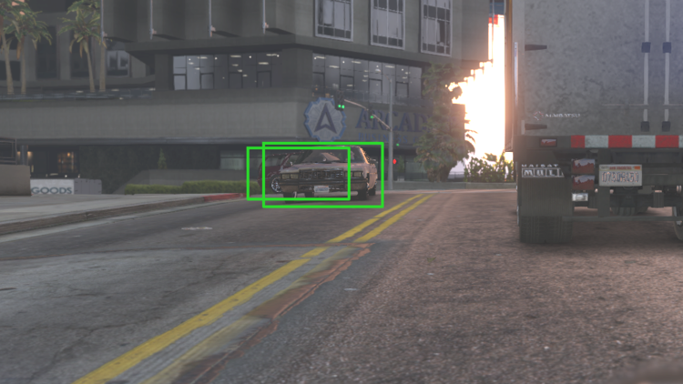
Figure 6: Left: Final detections without vg-NMS. Right: Final detections with vg-NMS.

A.2.3 Synscapes

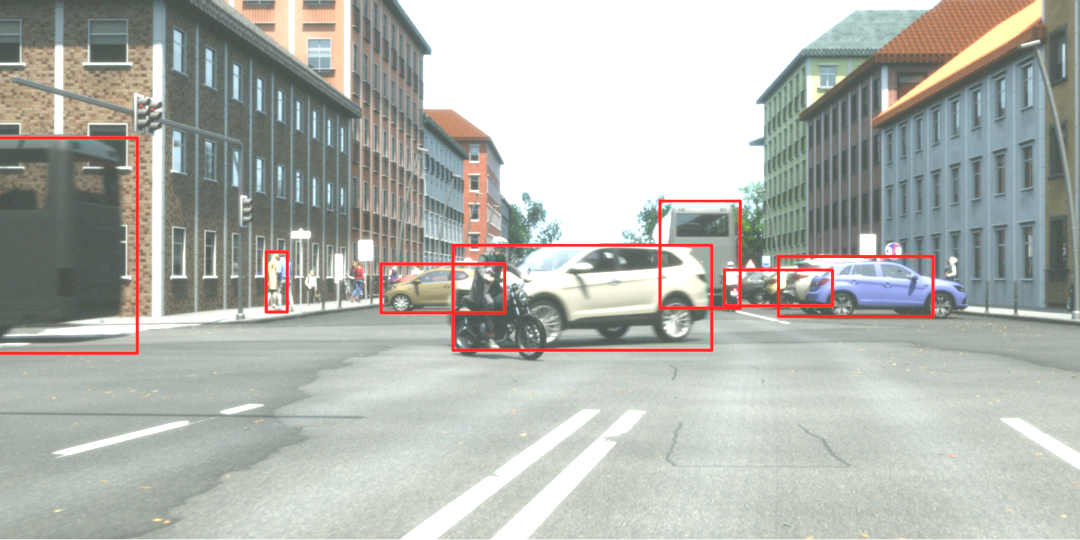
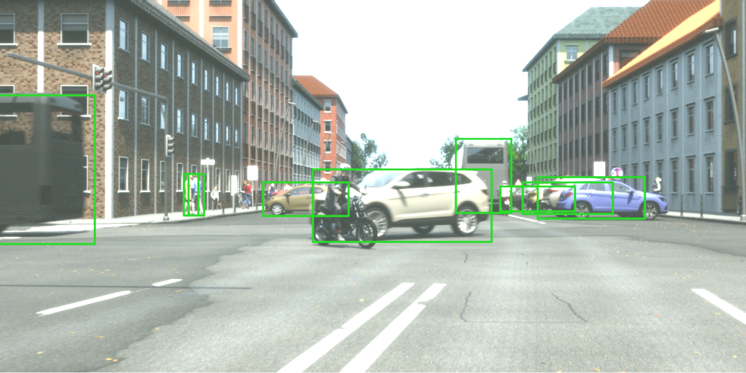
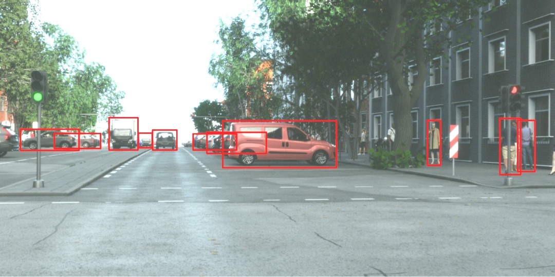
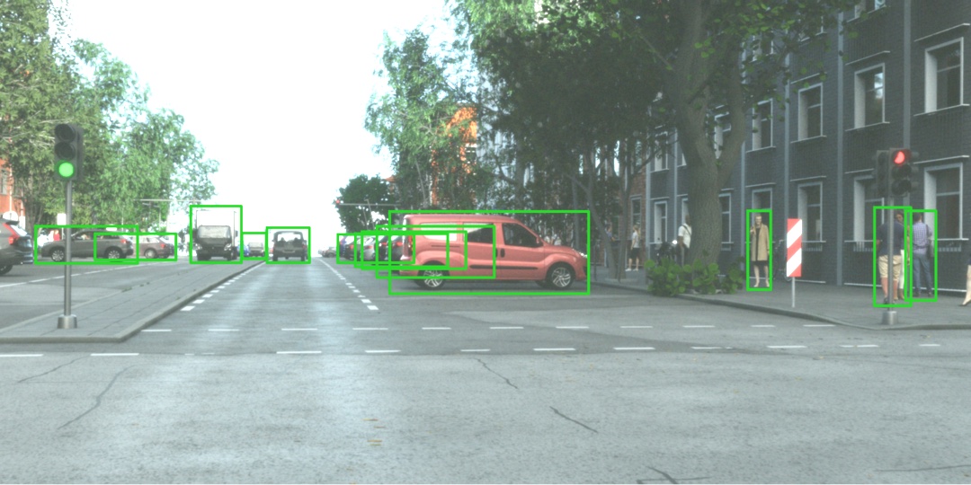
Figure 7: Left: Final detections without vg-NMS. Right: Final detections with vg-NMS.

References

- way [2019] Waymo open dataset: An autonomous driving dataset. https://waymo.com/open/, 2019.
- Bodla et al. [2017] Navaneeth Bodla, Bharat Singh, Rama Chellappa, and Larry S Davis. Soft-nms – improving object detection with one line of code. In Proceedings of the IEEE International Conference on Computer Vision, pages 5561–5569, 2017.
- Caesar et al. [2019] Holger Caesar, Varun Bankiti, Alex H. Lang, Sourabh Vora, Venice Erin Liong, Qiang Xu, Anush Krishnan, Yu Pan, Giancarlo Baldan, and Oscar Beijbom. nuscenes: A multimodal dataset for autonomous driving. arXiv preprint arXiv:1903.11027, 2019.
- Cao et al. [2018] Guimei Cao, Xuemei Xie, Wenzhe Yang, Quan Liao, Guangming Shi, and Jinjian Wu. Feature-fused ssd: fast detection for small objects. In Ninth International Conference on Graphic and Image Processing. International Society for Optics and Photonics, 2018.
- Caruana [1997] Rich Caruana. Multitask learning. Machine learning, 28(1):41–75, 1997.
- Cordts et al. [2016] Marius Cordts, Mohamed Omran, Sebastian Ramos, Timo Rehfeld, Markus Enzweiler, Rodrigo Benenson, Uwe Franke, Stefan Roth, and Bernt Schiele. The cityscapes dataset for semantic urban scene understanding. In Proceedings of the IEEE Conference on Computer Vision and Pattern Recognition, pages 3213–3223, 2016.
- Couprie et al. [2013] Camille Couprie, Clément Farabet, Laurent Najman, and Yann LeCun. Indoor semantic segmentation using depth information. arXiv preprint arXiv:1301.3572, 2013.
- Deng and Latecki [2017] Zhuo Deng and Jan Longin Latecki. Amodal detection of 3d objects: Inferring 3d bounding boxes from 2d ones in rgb-depth images. In Proceedings of the IEEE Conference on Computer Vision and Pattern Recognition, pages 5762–5770, 2017.
- Ehsani et al. [2018] Kiana Ehsani, Roozbeh Mottaghi, and Ali Farhadi. Segan: Segmenting and generating the invisible. In Proceedings of the IEEE Conference on Computer Vision and Pattern Recognition, pages 6144–6153, 2018.
- Follmann et al. [2019] Patrick Follmann, Rebecca König, Philipp Härtinger, Michael Klostermann, and Tobias Böttger. Learning to see the invisible: End-to-end trainable amodal instance segmentation. In 2019 IEEE Winter Conference on Applications of Computer Vision, pages 1328–1336, 2019.
- Fu et al. [2017] Cheng-Yang Fu, Wei Liu, Ananth Ranga, Ambrish Tyagi, and Alexander C Berg. Dssd: Deconvolutional single shot detector. arXiv preprint arXiv:1701.06659, 2017.
- Gählert et al. [2018] Nils Gählert, Marina Mayer, Lukas Schneider, Uwe Franke, and Joachim Denzler. Mb-net: Mergeboxes for real-time 3d vehicles detection. In 2018 IEEE Intelligent Vehicles Symposium, pages 2117–2124, 2018.
- Gählert et al. [2019] Nils Gählert, Jun-Jun Wan, Michael Weber, J. Marius Zöllner, Uwe Franke, and Joachim Denzler. Beyond bounding boxes: Using bounding shapes for real-time 3d vehicle detection from monocular rgb images. In 2019 IEEE Intelligent Vehicles Symposium, pages 675–682, 2019.
- Geiger et al. [2012] Andreas Geiger, Philip Lenz, and Raquel Urtasun. Are we ready for autonomous driving? the kitti vision benchmark suite. In 2012 IEEE Conference on Computer Vision and Pattern Recognition, pages 3354–3361, 2012.
- Girshick [2015] Ross Girshick. Fast r-cnn. In Proceedings of the IEEE International Conference on Computer Vision, pages 1440–1448, 2015.
- Girshick et al. [2014] Ross Girshick, Jeff Donahue, Trevor Darrell, and Jitendra Malik. Rich feature hierarchies for accurate object detection and semantic segmentation. In Proceedings of the IEEE Conference on Computer Vision and Pattern Recognition, pages 580–587, 2014.
- He et al. [2017] Kaiming He, Georgia Gkioxari, Piotr Dollár, and Ross Girshick. Mask r-cnn. In Proceedings of the IEEE International Conference on Computer Vision, pages 2961–2969, 2017.
- He et al. [2018] Yihui He, Xiangyu Zhang, Marios Savvides, and Kris Kitani. Softer-nms: Rethinking bounding box regression for accurate object detection. arXiv preprint arXiv:1809.08545, 2018.
- He et al. [2019] Yihui He, Chenchen Zhu, Jianren Wang, Marios Savvides, and Xiangyu Zhang. Bounding box regression with uncertainty for accurate object detection. In Proceedings of the IEEE Conference on Computer Vision and Pattern Recognition, pages 2888–2897, 2019.
- Hosang et al. [2016] Jan Hosang, Rodrigo Benenson, and Bernt Schiele. A convnet for non-maximum suppression. In German Conference on Pattern Recognition, pages 192–204. Springer, 2016.
- Hosang et al. [2017] Jan Hosang, Rodrigo Benenson, and Bernt Schiele. Learning non-maximum suppression. In Proceedings of the IEEE Conference on Computer Vision and Pattern Recognition, pages 4507–4515, 2017.
- Huang et al. [2018] Xinyu Huang, Xinjing Cheng, Qichuan Geng, Binbin Cao, Dingfu Zhou, Peng Wang, Yuanqing Lin, and Ruigang Yang. The apolloscape dataset for autonomous driving. In Proceedings of the IEEE Conference on Computer Vision and Pattern Recognition Workshops, pages 954–960, 2018.
- Kesten et al. [2019] R. Kesten, M. Usman, J. Houston, T. Pandya, K. Nadhamuni, A. Ferreira, M. Yuan, B. Low, A. Jain, P. Ondruska, S. Omari, S. Shah, A. Kulkarni, A. Kazakova, C. Tao, L. Platinsky, W. Jiang, and V. Shet. Lyft level 5 av dataset 2019. https://level5.lyft.com/dataset/, 2019.
- Kingma and Ba [2014] Diederik P Kingma and Jimmy Ba. Adam: A method for stochastic optimization. arXiv preprint arXiv:1412.6980, 2014.
- Li and Malik [2016] Ke Li and Jitendra Malik. Amodal instance segmentation. In European Conference on Computer Vision, pages 677–693. Springer, 2016.
- Lin et al. [2017] Tsung-Yi Lin, Priya Goyal, Ross Girshick, Kaiming He, and Piotr Dollár. Focal loss for dense object detection. In Proceedings of the IEEE International Conference on Computer Vision, pages 2980–2988, 2017.
- Liu et al. [2019] Songtao Liu, Di Huang, and Yunhong Wang. Adaptive nms: Refining pedestrian detection in a crowd. In Proceedings of the IEEE Conference on Computer Vision and Pattern Recognition, pages 6459–6468, 2019.
- Liu et al. [2016] Wei Liu, Dragomir Anguelov, Dumitru Erhan, Christian Szegedy, Scott Reed, Cheng-Yang Fu, and Alexander C Berg. Ssd: Single shot multibox detector. In European Conference on Computer Vision, pages 21–37. Springer, 2016.
- Mousavian et al. [2017] Arsalan Mousavian, Dragomir Anguelov, John Flynn, and Jana Kosecka. 3d bounding box estimation using deep learning and geometry. In Proceedings of the IEEE Conference on Computer Vision and Pattern Recognition, pages 7074–7082, 2017.
- Neuhold et al. [2017] Gerhard Neuhold, Tobias Ollmann, Samuel Rota Bulo, and Peter Kontschieder. The mapillary vistas dataset for semantic understanding of street scenes. In Proceedings of the IEEE International Conference on Computer Vision, pages 4990–4999, 2017.
- Qi et al. [2019] Lu Qi, Li Jiang, Shu Liu, Xiaoyong Shen, and Jiaya Jia. Amodal instance segmentation with kins dataset. In Proceedings of the IEEE Conference on Computer Vision and Pattern Recognition, pages 3014–3023, 2019.
- Redmon and Farhadi [2017] Joseph Redmon and Ali Farhadi. Yolo9000: better, faster, stronger. In Proceedings of the IEEE Conference on Computer Vision and Pattern Recognition, pages 7263–7271, 2017.
- Redmon and Farhadi [2018] Joseph Redmon and Ali Farhadi. Yolov3: An incremental improvement. arXiv preprint arXiv:1804.02767, 2018.
- Redmon et al. [2016] Joseph Redmon, Santosh Divvala, Ross Girshick, and Ali Farhadi. You only look once: Unified, real-time object detection. In Proceedings of the IEEE Conference on Computer Vision and Pattern Recognition, pages 779–788, 2016.
- Ren et al. [2015] Shaoqing Ren, Kaiming He, Ross Girshick, and Jian Sun. Faster r-cnn: Towards real-time object detection with region proposal networks. In Advances in Neural Information Processing Systems, pages 91–99, 2015.
- Rezatofighi et al. [2019] Hamid Rezatofighi, Nathan Tsoi, JunYoung Gwak, Amir Sadeghian, Ian Reid, and Silvio Savarese. Generalized intersection over union: A metric and a loss for bounding box regression. In Proceedings of the IEEE Conference on Computer Vision and Pattern Recognition, pages 658–666, 2019.
- Richter et al. [2017] Stephan R Richter, Zeeshan Hayder, and Vladlen Koltun. Playing for benchmarks. In Proceedings of the IEEE International Conference on Computer Vision, pages 2213–2222, 2017.
- Ros et al. [2016] German Ros, Laura Sellart, Joanna Materzynska, David Vazquez, and Antonio M Lopez. The synthia dataset: A large collection of synthetic images for semantic segmentation of urban scenes. In Proceedings of the IEEE Conference on Computer Vision and Pattern Recognition, pages 3234–3243, 2016.
- Szegedy et al. [2015] Christian Szegedy, Wei Liu, Yangqing Jia, Pierre Sermanet, Scott Reed, Dragomir Anguelov, Dumitru Erhan, Vincent Vanhoucke, and Andrew Rabinovich. Going deeper with convolutions. In Proceedings of the IEEE Conference on Computer Vision and Pattern Recognition, pages 1–9, 2015.
- Tychsen-Smith and Petersson [2018] Lachlan Tychsen-Smith and Lars Petersson. Improving object localization with fitness nms and bounded iou loss. In Proceedings of the IEEE Conference on Computer Vision and Pattern Recognition, pages 6877–6885, 2018.
- Weber et al. [2019] Michael Weber, Michael Fürst, and J Marius Zöllner. Direct 3d detection of vehicles in monocular images with a cnn based 3d decoder. In 2019 IEEE Intelligent Vehicles Symposium, pages 417–423, 2019.
- Wrenninge and Unger [2018] Magnus Wrenninge and Jonas Unger. Synscapes: A photorealistic synthetic dataset for street scene parsing. arXiv preprint arXiv:1810.08705, 2018.
- Xiang et al. [2015] Yu Xiang, Wongun Choi, Yuanqing Lin, and Silvio Savarese. Data-driven 3d voxel patterns for object category recognition. In Proceedings of the IEEE Conference on Computer Vision and Pattern Recognition, pages 1903–1911, 2015.
- Yu et al. [2018] Fisher Yu, Wenqi Xian, Yingying Chen, Fangchen Liu, Mike Liao, Vashisht Madhavan, and Trevor Darrell. Bdd100k: A diverse driving video database with scalable annotation tooling. arXiv preprint arXiv:1805.04687, 2018.
- Zhu et al. [2017] Yan Zhu, Yuandong Tian, Dimitris Metaxas, and Piotr Dollár. Semantic amodal segmentation. In Proceedings of the IEEE Conference on Computer Vision and Pattern Recognition, pages 1464–1472, 2017.