\newsiamremark

remarkRemark \newsiamremarkhypothesisHypothesis \newsiamthmclaimClaim \headersAEM Methods for Matrix EquationsK. Lee, H. C. Elman, C. E. Powell, and D. Lee \externaldocumentex_supplement

Alternating Energy Minimization Methods for Multi-term Matrix Equations

Kookjin Lee Extreme Scale Data Science and Analytics Department, Sandia National Laboratories (). koolee@sandia.gov    Howard C. Elman Department of Computer Science, University of Maryland, College Park (). elman@cs.umd.edu    Catherine E. Powell Department of Mathematics, University of Manchester, UK (). c.powell@manchester.ac.uk    Dongeun Lee Department of Computer Science, Texas A&M University-Commerce (). dongeun.lee@tamuc.edu
Abstract

We develop computational methods for approximating the solution of a linear multi-term matrix equation in low rank. We follow an alternating minimization framework, where the solution is represented as a product of two matrices, and approximations to each matrix are sought by solving certain minimization problems repeatedly. The solution methods we present are based on a rank-adaptive variant of alternating energy minimization methods that builds an approximation iteratively by successively computing a rank-one solution component at each step. We also develop efficient procedures to improve the accuracy of the low-rank approximate solutions computed using these successive rank-one update techniques. We explore the use of the methods with linear multi-term matrix equations that arise from stochastic Galerkin finite element discretizations of parameterized linear elliptic PDEs, and demonstrate their effectiveness with numerical studies.

keywords:
low-rank approximation, alternating energy minimization, stochastic Galerkin methods, matrix equations
{AMS}

35R60, 60H35, 65F10, 65N30

1 Introduction

We are interested in computing a low-rank approximate solution of a Kronecker-product structured linear system Au=b𝐴𝑢𝑏Au=b,

(1) (i=0mGiKi)u=i=0rgifi,superscriptsubscript𝑖0𝑚tensor-productsubscript𝐺𝑖subscript𝐾𝑖𝑢superscriptsubscript𝑖0𝑟tensor-productsubscript𝑔𝑖subscript𝑓𝑖\left(\sum_{i=0}^{m}G_{i}\otimes K_{i}\right)u=\sum_{i=0}^{r}g_{i}\otimes f_{i},

where A=i=0mGiKi𝐴superscriptsubscript𝑖0𝑚tensor-productsubscript𝐺𝑖subscript𝐾𝑖A=\sum_{i=0}^{m}G_{i}\otimes K_{i} is symmetric positive definite, tensor-product\otimes is the Kronecker product, {Ki}i=0mn1×n1superscriptsubscriptsubscript𝐾𝑖𝑖0𝑚superscriptsubscript𝑛1subscript𝑛1\{K_{i}\}_{i=0}^{m}\in\mathbb{R}^{n_{1}\times n_{1}}, {Gi}i=0mn2×n2superscriptsubscriptsubscript𝐺𝑖𝑖0𝑚superscriptsubscript𝑛2subscript𝑛2\{G_{i}\}_{i=0}^{m}\in\mathbb{R}^{n_{2}\times n_{2}}, {fi}i=0rn1superscriptsubscriptsubscript𝑓𝑖𝑖0𝑟superscriptsubscript𝑛1\{f_{i}\}_{i=0}^{r}\in\mathbb{R}^{n_{1}}, and {gi}i=0rn2superscriptsubscriptsubscript𝑔𝑖𝑖0𝑟superscriptsubscript𝑛2\{g_{i}\}_{i=0}^{r}\in\mathbb{R}^{n_{2}}. Systems with such structure arise in the discretization of linear elliptic PDEs in high dimensions [2, 18, 19, 20] and stochastic Galerkin finite element discretization of parameterized linear elliptic PDEs [11, 22, 25, 38]. The solution vector un1n2𝑢superscriptsubscript𝑛1subscript𝑛2u\in\mathbb{R}^{n_{1}n_{2}} consists of n2subscript𝑛2n_{2} subvectors of dimension n1subscript𝑛1n_{1}, i.e., u=[u1𝖳,,un2𝖳]𝖳𝑢superscriptsuperscriptsubscript𝑢1𝖳superscriptsubscript𝑢subscript𝑛2𝖳𝖳u=[u_{1}^{\mathsf{T}},\ldots,u_{n_{2}}^{\mathsf{T}}]^{\mathsf{T}}, where {ui}i=1n2n1superscriptsubscriptsubscript𝑢𝑖𝑖1subscript𝑛2superscriptsubscript𝑛1\{u_{i}\}_{i=1}^{n_{2}}\in\mathbb{R}^{n_{1}}. It also has an alternative representation in matrix format, U=[u1,,un2]n1×n2𝑈subscript𝑢1subscript𝑢subscript𝑛2superscriptsubscript𝑛1subscript𝑛2U=[u_{1},\ldots,u_{n_{2}}]\in\mathbb{R}^{n_{1}\times n_{2}}, for which the system equivalent to (1) is the linear multi-term matrix equation [31]

(2) i=0mKiUGi𝖳=B,superscriptsubscript𝑖0𝑚subscript𝐾𝑖𝑈superscriptsubscript𝐺𝑖𝖳𝐵\sum_{i=0}^{m}K_{i}UG_{i}^{\mathsf{T}}=B,

where B=i=0rfigi𝖳n1×n2𝐵superscriptsubscript𝑖0𝑟subscript𝑓𝑖superscriptsubscript𝑔𝑖𝖳superscriptsubscript𝑛1subscript𝑛2B=\sum_{i=0}^{r}f_{i}g_{i}^{\mathsf{T}}\in\mathbb{R}^{n_{1}\times n_{2}} and it is assumed that m,rn1,n2formulae-sequencemuch-less-than𝑚𝑟subscript𝑛1subscript𝑛2m,r\ll n_{1},n_{2}. The system matrices Kisubscript𝐾𝑖K_{i} and Gisubscript𝐺𝑖G_{i} obtained from discretization methods are typically sparse and, thus, for moderately large system matrices, Krylov subspace methods [29, 30] and multigrid methods [3, 9, 21] have been natural choices to solve such systems.

The dimensions of the system matrices grow rapidly, however, if a solution is sought on a refined grid or (in the case of stochastic Galerkin methods) if the so-called parametric space is high-dimensional. For large n1subscript𝑛1n_{1} and n2subscript𝑛2n_{2}, direct applications of standard iterative methods may be computationally prohibitive and storing or explicitly forming the matrix U𝑈U may be prohibitive in terms of memory. Instead of computing an exact solution of (2), we are interested in inexpensive computation of an approximate solution of low rank. To achieve this goal, we begin by introducing a factored representation of Un1×n2𝑈superscriptsubscript𝑛1subscript𝑛2U\in\mathbb{R}^{n_{1}\times n_{2}},

U=VW𝖳,𝑈𝑉superscript𝑊𝖳U=VW^{\mathsf{T}},

where, if U𝑈U is of full rank m:=min(n1,n2)assign𝑚subscript𝑛1subscript𝑛2m:=\min(n_{1},n_{2}), Vn1×m𝑉superscriptsubscript𝑛1𝑚V\in\mathbb{R}^{n_{1}\times m} and Wn2×m𝑊superscriptsubscript𝑛2𝑚W\in\mathbb{R}^{n_{2}\times m}. Our aim is to find a low-rank approximation to this factored matrix of the form

(3) Up=VpWp𝖳n1×n2,subscript𝑈𝑝subscript𝑉𝑝superscriptsubscript𝑊𝑝𝖳superscriptsubscript𝑛1subscript𝑛2U_{p}=V_{p}W_{p}^{\mathsf{T}}\in\mathbb{R}^{n_{1}\times n_{2}},

where Vp=[v1,,vp]n1×psubscript𝑉𝑝subscript𝑣1subscript𝑣𝑝superscriptsubscript𝑛1𝑝V_{p}=[v_{1},\ldots,v_{p}]\in\mathbb{R}^{n_{1}\times p} and Wp=[w1,,wp]n2×psubscript𝑊𝑝subscript𝑤1subscript𝑤𝑝superscriptsubscript𝑛2𝑝W_{p}=[w_{1},\ldots,w_{p}]\in\mathbb{R}^{n_{2}\times p} and pmmuch-less-than𝑝𝑚p\ll m, and we want to derive solution algorithms for computing Upsubscript𝑈𝑝U_{p} that operate only on the factors Vpsubscript𝑉𝑝V_{p} and Wpsubscript𝑊𝑝W_{p} without explicitly forming Upsubscript𝑈𝑝U_{p}.

One such solution algorithm has been developed for matrix completion/sensing [14, 16], which, at the p𝑝pth iteration, computes Vpsubscript𝑉𝑝V_{p} and Wpsubscript𝑊𝑝W_{p} by alternately solving certain minimization problems. Although the algorithm computes highly accurate approximations, it can become very expensive as p𝑝p increases. Another approach is to use successive rank-one approximations and successively compute pairs of vectors {(vi\{(v_{i},wi)}i=1pw_{i})\}_{i=1}^{p} to build the factors Vpsubscript𝑉𝑝V_{p} and Wpsubscript𝑊𝑝W_{p} of (3) until a stopping criterion is satisfied. The p𝑝pth iteration starts with Vp1subscript𝑉𝑝1V_{p-1} and Wp1subscript𝑊𝑝1W_{p-1} and constructs vpsubscript𝑣𝑝v_{p} and wpsubscript𝑤𝑝w_{p} as the solutions of certain minimization problems. This approach for solving parameterized PDEs is one component of a methodology known as Proper Generalized Decomposition (PGD) [26, 27, 37]. As observed in those works, using only successive rank-one approximations is less expensive but may not be practical because it typically results in approximate solutions with an unnecessarily large value of p𝑝p for satisfying a certain error tolerance.

Our goal in this study is to develop solution algorithms that preserve only the good properties of the above two types of solution strategies, i.e., algorithms that compute an accurate solution in a computationally efficient way. In developing such algorithms, we take our cue from PGD methods, in which, to improve accuracy, the successive rank-one constructions are supplemented with an updating procedure that is performed intermittently during the iteration. Inspired by this approach, we propose a solution algorithm that adaptively computes approximate solutions in an inexpensive way via the successive rank-one approximation method. This is then supplemented by an enhancement procedure, which effectively improves the accuracy of the resulting approximate solutions. We propose two novel enhancement procedures developed by modifying some ideas used for matrix completion problems [16].

Some other rank-adaptive approaches for approximating solutions of parameterized or high-dimensional PDEs in low-rank format are as follows. A method in [4] uses alternating energy minimization techniques in combination with tensor-train decompositions [28]. One can incrementally compute rank-one solution pairs by solving a residual minimization problem, an approach known as alternating least-squares (ALS) methods, which has been used to compute low-rank approximate solutions of parameterized PDEs in [5, 6], and to solve matrix recovery problems, matrix sensing and completion problems, [13, 14, 16, 32]. In [31], an adaptive iterative procedure to solve the matrix equation (2) is given, which incrementally computes a set of orthonormal basis vectors for use in representing the spatial part of the solution, Vpsubscript𝑉𝑝V_{p}. See [36] for an overview of other computational approaches for solving linear matrix equations.

An outline of the paper is as follows. In Section 2, we introduce and derive alternating energy minimization (AEM) methods using the well-known general projection framework and discuss a collection of methods developed for constructing low-rank approximate solutions of the form (3). In Section 3, we discuss enhancement procedures and derive two new approaches for performing such updates. In Section 4, we measure the effectiveness and the efficiency of the variants of the methods with numerical experiments. Finally, in Section 5, we draw some conclusions.

2 Alternating energy minimization (AEM) methods

In this section, we derive AEM methods for solving the matrix equation (2) from the optimal projection framework, and review two variants of such methods. We first introduce some notation. Capital and small letters are used to denote matrices and vectors, respectively. As a special case, a zero-column matrix is indicated by using a subscript 0, e.g., X0n1×0subscript𝑋0superscriptsubscript𝑛10X_{0}\in\mathbb{R}^{n_{1}\times 0}. An inner product between two matrices X,Yn1×n2𝑋𝑌superscriptsubscript𝑛1subscript𝑛2X,Y\in\mathbb{R}^{n_{1}\times n_{2}} is defined as X,Ytr(X𝖳Y)=tr(XY𝖳)=i,jXijYij𝑋𝑌trsuperscript𝑋𝖳𝑌tr𝑋superscript𝑌𝖳subscript𝑖𝑗subscript𝑋𝑖𝑗subscript𝑌𝑖𝑗\langle X,Y\rangle\equiv\text{tr}(X^{\mathsf{T}}Y)=\text{tr}(XY^{\mathsf{T}})=\sum_{i,j}X_{ij}Y_{ij}, where tr is the trace operator, and tr(X)=i=1nxiitr𝑋superscriptsubscript𝑖1𝑛subscript𝑥𝑖𝑖\text{tr}(X)=\sum_{i=1}^{n}x_{ii} if Xn×n𝑋superscript𝑛𝑛X\in\mathbb{R}^{n\times n}. The norm induced by ,\langle\cdot,\cdot\rangle is the Frobenius norm XF=X,Xsubscriptnorm𝑋F𝑋𝑋\|X\|_{\text{F}}=\sqrt{\langle X,X\rangle}. For shorthand notation, we introduce a linear operator 𝒜(X)=i=0mKiXGi𝖳𝒜𝑋superscriptsubscript𝑖0𝑚subscript𝐾𝑖𝑋superscriptsubscript𝐺𝑖𝖳\mathcal{A}(X)=\sum_{i=0}^{m}K_{i}XG_{i}^{\mathsf{T}} for Xn1×n2𝑋superscriptsubscript𝑛1subscript𝑛2X\in\mathbb{R}^{n_{1}\times n_{2}}. Using this, we can define the weighted inner product X,YA=𝒜(X),Y=X,𝒜(Y)subscript𝑋𝑌𝐴𝒜𝑋𝑌𝑋𝒜𝑌\langle X,Y\rangle_{A}=\langle\mathcal{A}(X),Y\rangle=\langle X,\mathcal{A}(Y)\rangle and the induced A𝐴A-norm A\|\cdot\|_{A}. Finally, vec denotes a vectorization operator, vec(X)=xvec𝑋𝑥\text{vec}(X)=x, where X=[x1,,xn2]n1×n2𝑋subscript𝑥1subscript𝑥subscript𝑛2superscriptsubscript𝑛1subscript𝑛2X=[x_{1},\ldots,x_{n_{2}}]\in\mathbb{R}^{n_{1}\times n_{2}} and x=[x1𝖳,,xn2𝖳]𝖳n1n2𝑥superscriptsuperscriptsubscript𝑥1𝖳superscriptsubscript𝑥subscript𝑛2𝖳𝖳superscriptsubscript𝑛1subscript𝑛2x=[x_{1}^{\mathsf{T}},\ldots,x_{n_{2}}^{\mathsf{T}}]^{\mathsf{T}}\in\mathbb{R}^{n_{1}n_{2}}, where xin1subscript𝑥𝑖superscriptsubscript𝑛1x_{i}\in\mathbb{R}^{n_{1}}, for i=1,,n2𝑖1subscript𝑛2i=1,\ldots,n_{2}.

2.1 General projection framework

For the computation of Vpsubscript𝑉𝑝V_{p} and Wpsubscript𝑊𝑝W_{p} in (3), we rely on the classical theory of orthogonal (Galerkin) projection methods [33, Proposition 5.2]. Let 𝒦n1×n2𝒦superscriptsubscript𝑛1subscript𝑛2\mathcal{K}\subset\mathbb{R}^{n_{1}\times n_{2}} be a search space in which an approximate solution Upn1×n2subscript𝑈𝑝superscriptsubscript𝑛1subscript𝑛2U_{p}\in\mathbb{R}^{n_{1}\times n_{2}} is sought, and let \mathcal{L} be a constraint space onto which the residual B𝒜(Up)𝐵𝒜subscript𝑈𝑝B-\mathcal{A}(U_{p}) is projected. Following [33, Proposition 5.2], if the system matrix A𝐴A is symmetric positive definite and =𝒦𝒦\mathcal{L}=\mathcal{K}, then a matrix Upsuperscriptsubscript𝑈𝑝U_{p}^{\ast} is the result of an orthogonal projection onto \mathcal{L} if and only if it minimizes the A𝐴A-norm of the error over 𝒦𝒦\mathcal{K}, i.e.,

Up=argminUp𝒦JA(Up),superscriptsubscript𝑈𝑝subscript𝑈𝑝𝒦subscript𝐽𝐴subscript𝑈𝑝U_{p}^{\ast}=\underset{U_{p}\in\mathcal{K}}{\arg\min}\>J_{A}(U_{p}),

where the objective function is

(4) JA(Up)=12UUpA2.subscript𝐽𝐴subscript𝑈𝑝12superscriptsubscriptnorm𝑈subscript𝑈𝑝𝐴2J_{A}(U_{p})=\frac{1}{2}\|U-U_{p}\|_{A}^{2}.

Because we seek a factored representation of Upsubscript𝑈𝑝U_{p}, we slightly modify (4) to give

(5) JA(Vp,Wp)=12UVpWp𝖳A2,subscript𝐽𝐴subscript𝑉𝑝subscript𝑊𝑝12superscriptsubscriptnorm𝑈subscript𝑉𝑝superscriptsubscript𝑊𝑝𝖳𝐴2J_{A}(V_{p},W_{p})=\frac{1}{2}\|U-V_{p}W_{p}^{\mathsf{T}}\|_{A}^{2},

and obtain a new minimization problem

(6) minVpn1×p,Wpn2×pJA(Vp,Wp).subscriptformulae-sequencesubscript𝑉𝑝superscriptsubscript𝑛1𝑝subscript𝑊𝑝superscriptsubscript𝑛2𝑝subscript𝐽𝐴subscript𝑉𝑝subscript𝑊𝑝\min_{V_{p}\in\mathbb{R}^{n_{1}\times p},W_{p}\in\mathbb{R}^{n_{2}\times p}}J_{A}(V_{p},W_{p}).

Since JAsubscript𝐽𝐴J_{A} is quadratic, gradients with respect to Vpsubscript𝑉𝑝V_{p} and Wpsubscript𝑊𝑝W_{p} can be easily obtained as

(7) VpJAsubscriptsubscript𝑉𝑝subscript𝐽𝐴\displaystyle\nabla_{V_{p}}J_{A} =(𝒜(VpWp𝖳)B)Wp=i=0m(KiVpWp𝖳Gi𝖳)WpBWp,absent𝒜subscript𝑉𝑝superscriptsubscript𝑊𝑝𝖳𝐵subscript𝑊𝑝superscriptsubscript𝑖0𝑚subscript𝐾𝑖subscript𝑉𝑝superscriptsubscript𝑊𝑝𝖳superscriptsubscript𝐺𝑖𝖳subscript𝑊𝑝𝐵subscript𝑊𝑝\displaystyle=\left(\mathcal{A}(V_{p}W_{p}^{\mathsf{T}})-B\right)W_{p}=\sum_{i=0}^{m}(K_{i}V_{p}W_{p}^{\mathsf{T}}G_{i}^{\mathsf{T}})W_{p}-BW_{p},
(8) WpJAsubscriptsubscript𝑊𝑝subscript𝐽𝐴\displaystyle\nabla_{W_{p}}J_{A} =(𝒜(VpWp𝖳)B)𝖳Vp=i=0m(KiVpWp𝖳Gi𝖳)𝖳VpB𝖳Vp.absentsuperscript𝒜subscript𝑉𝑝superscriptsubscript𝑊𝑝𝖳𝐵𝖳subscript𝑉𝑝superscriptsubscript𝑖0𝑚superscriptsubscript𝐾𝑖subscript𝑉𝑝superscriptsubscript𝑊𝑝𝖳superscriptsubscript𝐺𝑖𝖳𝖳subscript𝑉𝑝superscript𝐵𝖳subscript𝑉𝑝\displaystyle=\left(\mathcal{A}(V_{p}W_{p}^{\mathsf{T}})-B\right)^{\mathsf{T}}V_{p}=\sum_{i=0}^{m}(K_{i}V_{p}W_{p}^{\mathsf{T}}G_{i}^{\mathsf{T}})^{\mathsf{T}}V_{p}-B^{\mathsf{T}}V_{p}.

Employing the first-order optimality condition on (7)–(8) (i.e., setting (7) and (the transpose of) (8) to be zero) results in the set of equations

(9) i=0m(KiVpWp𝖳Gi𝖳)Wpsuperscriptsubscript𝑖0𝑚subscript𝐾𝑖subscript𝑉𝑝superscriptsubscript𝑊𝑝𝖳superscriptsubscript𝐺𝑖𝖳subscript𝑊𝑝\displaystyle\sum_{i=0}^{m}(K_{i}V_{p}W_{p}^{\mathsf{T}}G_{i}^{\mathsf{T}})W_{p} =BWpn1×p,absent𝐵subscript𝑊𝑝superscriptsubscript𝑛1𝑝\displaystyle=BW_{p}\in\mathbb{R}^{n_{1}\times p},
(10) i=0mVp𝖳(KiVpWp𝖳Gi𝖳)superscriptsubscript𝑖0𝑚superscriptsubscript𝑉𝑝𝖳subscript𝐾𝑖subscript𝑉𝑝superscriptsubscript𝑊𝑝𝖳superscriptsubscript𝐺𝑖𝖳\displaystyle\sum_{i=0}^{m}V_{p}^{\mathsf{T}}(K_{i}V_{p}W_{p}^{\mathsf{T}}G_{i}^{\mathsf{T}}) =Vp𝖳Bp×n2.absentsuperscriptsubscript𝑉𝑝𝖳𝐵superscript𝑝subscript𝑛2\displaystyle=V_{p}^{\mathsf{T}}B\in\mathbb{R}^{p\times n_{2}}.

These equations can be interpreted as projections of the residual B𝒜(VpWp𝖳)𝐵𝒜subscript𝑉𝑝superscriptsubscript𝑊𝑝𝖳B-\mathcal{A}(V_{p}W_{p}^{\mathsf{T}}) onto the spaces spanned by the columns of Wpsubscript𝑊𝑝W_{p} and Vpsubscript𝑉𝑝V_{p}, respectively.

Given (9)–(10), a widely used strategy for solving the minimization problem (6) is to compute each component of the solution pair (Vp,Wp)subscript𝑉𝑝subscript𝑊𝑝(V_{p},W_{p}) alternately [4, 5, 6, 13, 14, 16]. That is, one can fix Wpsubscript𝑊𝑝W_{p} and solve the system of equations of order n1psubscript𝑛1𝑝n_{1}p in (9) for Vpsubscript𝑉𝑝V_{p}, and then one can fix Vpsubscript𝑉𝑝V_{p} and solve the system of equations of order n2psubscript𝑛2𝑝n_{2}p in (10) for Wpsubscript𝑊𝑝W_{p}. However, in this approach, suitable choices of p𝑝p for satisfying a fixed error tolerance are typically not known a priori. Thus, adaptive schemes that incrementally compute solution pairs (visubscript𝑣𝑖v_{i},wisubscript𝑤𝑖w_{i}) have been introduced [16, 26, 27, 37]. All of these schemes are based on alternately solving two systems of equations for two types of variables in an effort to minimize a certain error measure. In this study, we employ alternating methods for minimizing the energy norm of the error (6) and, thus, we refer to approaches of this type as alternating energy minimization (AEM) methods. In the following sections, we present two adaptive variants of AEM methods: a Stage-p𝑝p AEM method and a successive rank-one AEM method.

2.2 Stage-p𝑝p AEM method

An alternating minimization method that entails solving a sequence of least-squares problems whose dimensions increase with p𝑝p was developed in [16] for solving matrix-recovery problems [13, 14, 16]. We adapt this approach to the energy minimization problem (6) and refer to it as the Stage-p𝑝p  AEM method. It is an iterative method that runs until an approximate solution satisfies a stopping criterion (e.g., the relative residual B𝒜(VpWp𝖳)FϵBFsubscriptnorm𝐵𝒜subscript𝑉𝑝superscriptsubscript𝑊𝑝𝖳Fitalic-ϵsubscriptnorm𝐵F\|B-\mathcal{A}(V_{p}W_{p}^{\mathsf{T}})\|_{\text{F}}\leq\epsilon\|B\|_{\text{F}} with a user-specified stopping tolerance ϵitalic-ϵ\epsilon). At the p𝑝pth iteration, called a “stage” in [16], this method seeks p𝑝p-column factors Vpsubscript𝑉𝑝V_{p} and Wpsubscript𝑊𝑝W_{p} determining an approximate solution by initializing Wp(0)superscriptsubscript𝑊𝑝0W_{p}^{(0)} and solving the following systems of equations in sequence:

(11) i=0m(Ki)Vp(k)(Wp(k1)Gi𝖳Wp(k1))𝖳superscriptsubscript𝑖0𝑚subscript𝐾𝑖superscriptsubscript𝑉𝑝𝑘superscriptsuperscriptsubscript𝑊𝑝𝑘1superscriptsubscript𝐺𝑖𝖳superscriptsubscript𝑊𝑝𝑘1𝖳\displaystyle\sum_{i=0}^{m}(K_{i})V_{p}^{(k)}(W_{p}^{(k-1)}{}^{\mathsf{T}}G_{i}W_{p}^{(k-1)})^{\mathsf{T}} =BWp(k1),absent𝐵superscriptsubscript𝑊𝑝𝑘1\displaystyle=BW_{p}^{(k-1)},
(12) i=0m(Vp(k)Ki𝖳Vp(k))Wp(k)(Gi𝖳)𝖳\displaystyle\sum_{i=0}^{m}(V_{p}^{(k)}{}^{\mathsf{T}}K_{i}V_{p}^{(k)})W_{p}^{(k)}{}^{\mathsf{T}}(G_{i}^{\mathsf{T}}) =Vp(k)B𝖳,absentsuperscriptsubscript𝑉𝑝𝑘superscript𝐵𝖳\displaystyle=V_{p}^{(k)}{}^{\mathsf{T}}B,

for k=1,,kmax𝑘1subscript𝑘k=1,\ldots,k_{\max}, where the superscript indicates the number of alternations between the two systems of equations (11)–(12). Note that the method can also begin by initializing Vp(0)superscriptsubscript𝑉𝑝0V_{p}^{(0)} and alternating between (12) and (11). Algorithm 1 summarizes the entire procedure. For the initialization of Wp(0)superscriptsubscript𝑊𝑝0W_{p}^{(0)} (line 3), one step of the singular value projection method [15] is performed with the exact settings from [16, Algorithm 3]. The CheckConvergence procedure (line 9) is detailed in Section 3.

Algorithm 1 Stage-p𝑝p  AEM method

INPUT: pmaxsubscript𝑝p_{\max}: the maximum number of solution pairs,
                   kmaxsubscript𝑘k_{\max}: the maximum number of alternations in each stage,
                   ϵitalic-ϵ\epsilon: a parameter for checking convergence,

1:function StagepAEM(pmax,kmax,ϵsubscript𝑝subscript𝑘italic-ϵp_{\max},k_{\max},\epsilon)
2:     for  p=1,,pmax𝑝1subscript𝑝p=1,\ldots,p_{\max} do
3:         [Vp(0),Wp(0)]=superscriptsubscript𝑉𝑝0superscriptsubscript𝑊𝑝0absent[V_{p}^{(0)},W_{p}^{(0)}]= first p𝑝p singular vectors of Vp1Wp1𝖳34(𝒜(Vp1Wp1𝖳)B)subscript𝑉𝑝1superscriptsubscript𝑊𝑝1𝖳34𝒜subscript𝑉𝑝1superscriptsubscript𝑊𝑝1𝖳𝐵V_{p-1}W_{p-1}^{\mathsf{T}}-\frac{3}{4}(\mathcal{A}(V_{p-1}W_{p-1}^{\mathsf{T}})\!-\!B)
4:         for  k=1,,kmax𝑘1subscript𝑘k=1,\ldots,k_{\max} do
5:              Vp(k)superscriptsubscript𝑉𝑝𝑘absentV_{p}^{(k)}\leftarrow solve (11)
6:              Wp(k)superscriptsubscript𝑊𝑝𝑘absentW_{p}^{(k)}\leftarrow solve (12)
7:         end for
8:         VpVp(k)subscript𝑉𝑝superscriptsubscript𝑉𝑝𝑘V_{p}\leftarrow V_{p}^{(k)} and WpWp(k)subscript𝑊𝑝superscriptsubscript𝑊𝑝𝑘W_{p}\leftarrow W_{p}^{(k)}
9:         Vp,Wpsubscript𝑉𝑝subscript𝑊𝑝absentV_{p},W_{p}\leftarrow CheckConvergence(Vp,Wp,ϵsubscript𝑉𝑝subscript𝑊𝑝italic-ϵV_{p},W_{p},\epsilon)
10:     end for
11:end function

Systems of equations for “vectorized” versions of the matrix factors Vpsubscript𝑉𝑝V_{p} and Wpsubscript𝑊𝑝W_{p} can be derived111The left-hand sides of (13)–(14) are derived using vec(KUG𝖳)=(GK)vec(U)vec𝐾𝑈superscript𝐺𝖳tensor-product𝐺𝐾vec𝑈\text{vec}(KUG^{\mathsf{T}})=(G\otimes K)\text{vec}(U). Note that (14) is derived by first transposing (12) and then vectorizing the resulting equation. In the sequel, vectorized versions of equations for the factor Wpsubscript𝑊𝑝W_{p} are derived by first taking the transpose. from (11) and (12) as follows

(13) i=0m[(Wp(k1)Gi𝖳Wp(k1))Ki]vec(Vp(k))superscriptsubscript𝑖0𝑚delimited-[]tensor-productsuperscriptsubscript𝑊𝑝𝑘1superscriptsubscript𝐺𝑖𝖳superscriptsubscript𝑊𝑝𝑘1subscript𝐾𝑖vecsuperscriptsubscript𝑉𝑝𝑘\displaystyle\sum_{i=0}^{m}[(W_{p}^{(k-1)}{}^{\mathsf{T}}G_{i}W_{p}^{(k-1)})\otimes K_{i}]\,\text{vec}(V_{p}^{(k)}) =vec(BWp(k1)),absentvec𝐵superscriptsubscript𝑊𝑝𝑘1\displaystyle=\text{vec}(BW_{p}^{(k-1)}),
(14) i=0m[(Vp(k)Ki𝖳Vp(k))Gi]vec(Wp(k))superscriptsubscript𝑖0𝑚delimited-[]tensor-productsuperscriptsubscript𝑉𝑝𝑘superscriptsubscript𝐾𝑖𝖳superscriptsubscript𝑉𝑝𝑘subscript𝐺𝑖vecsuperscriptsubscript𝑊𝑝𝑘\displaystyle\sum_{i=0}^{m}[(V_{p}^{(k)}{}^{\mathsf{T}}K_{i}V_{p}^{(k)})\otimes G_{i}]\,\text{vec}(W_{p}^{(k)}) =vec(B𝖳Vp(k)).absentvecsuperscript𝐵𝖳superscriptsubscript𝑉𝑝𝑘\displaystyle=\text{vec}(B^{\mathsf{T}}V_{p}^{(k)}{}).

Thus, solving (11) and (12) is equivalent to solving coupled linear systems with coefficient matrices of dimensions n1p×n1psubscript𝑛1𝑝subscript𝑛1𝑝n_{1}p\times n_{1}p and n2p×n2psubscript𝑛2𝑝subscript𝑛2𝑝n_{2}p\times n_{2}p, respectively, which are smaller than that of the original system (2) when p𝑝p is small. However, the reduced matrix factors (of size p×p𝑝𝑝p\times p) are dense, even if the original ones are sparse, and so as p𝑝p increases, the computational costs for solving (11)–(12) increase and the Stage-p𝑝p AEM method may be impractical for large-scale problems.

2.3 Successive rank-one AEM method

We now describe a successive rank-one (S-rank-111) approximation method which, at each iteration, adds a rank-one correction to the current iterate. This is a basic component of PGD methods [26, 27, 37] for solving parameterized PDEs. The method only requires solutions of linear systems with coefficient matrices of size n1×n1subscript𝑛1subscript𝑛1n_{1}\times n_{1} and n2×n2subscript𝑛2subscript𝑛2n_{2}\times n_{2} rather than coupled systems like those in the Stage-p𝑝p AEM method that grow in size with the step counter p𝑝p.

Assume that p1𝑝1p-1 pairs of solutions are computed, giving Vp1subscript𝑉𝑝1V_{p-1} and Wp1subscript𝑊𝑝1W_{p-1}. The next step is to compute a new solution pair (vp,wp)subscript𝑣𝑝subscript𝑤𝑝(v_{p},w_{p}) by choosing the objective function

JA(vp,wp)=12UVp1Wp1𝖳vpwp𝖳A2,subscript𝐽𝐴subscript𝑣𝑝subscript𝑤𝑝12superscriptsubscriptnorm𝑈subscript𝑉𝑝1superscriptsubscript𝑊𝑝1𝖳subscript𝑣𝑝superscriptsubscript𝑤𝑝𝖳𝐴2J_{A}(v_{p},w_{p})=\frac{1}{2}\|U-V_{p-1}W_{p-1}^{\mathsf{T}}-v_{p}w_{p}^{\mathsf{T}}\|_{A}^{2},

and solving the following minimization problem

minvpn1,wpn2JA(vp,wp).subscriptformulae-sequencesubscript𝑣𝑝superscriptsubscript𝑛1subscript𝑤𝑝superscriptsubscript𝑛2subscript𝐽𝐴subscript𝑣𝑝subscript𝑤𝑝\min_{v_{p}\in\mathbb{R}^{n_{1}},w_{p}\in\mathbb{R}^{n_{2}}}J_{A}(v_{p},w_{p}).

The gradients of JAsubscript𝐽𝐴J_{A} with respect to vpsubscript𝑣𝑝v_{p} and wpsubscript𝑤𝑝w_{p} are

(15) vpJAsubscriptsubscript𝑣𝑝subscript𝐽𝐴\displaystyle\nabla_{v_{p}}J_{A} =(𝒜(vpwp𝖳)+𝒜(Vp1Wp1𝖳)B)wp,absent𝒜subscript𝑣𝑝superscriptsubscript𝑤𝑝𝖳𝒜subscript𝑉𝑝1superscriptsubscript𝑊𝑝1𝖳𝐵subscript𝑤𝑝\displaystyle=\left(\mathcal{A}(v_{p}w_{p}^{\mathsf{T}})+\mathcal{A}(V_{p-1}W_{p-1}^{\mathsf{T}})-B\right)w_{p},
(16) wpJAsubscriptsubscript𝑤𝑝subscript𝐽𝐴\displaystyle\nabla_{w_{p}}J_{A} =(𝒜(vpwp𝖳)+𝒜(Vp1Wp1𝖳)B)𝖳vp.absentsuperscript𝒜subscript𝑣𝑝superscriptsubscript𝑤𝑝𝖳𝒜subscript𝑉𝑝1superscriptsubscript𝑊𝑝1𝖳𝐵𝖳subscript𝑣𝑝\displaystyle=\left(\mathcal{A}(v_{p}w_{p}^{\mathsf{T}})+\mathcal{A}(V_{p-1}W_{p-1}^{\mathsf{T}})-B\right)^{\mathsf{T}}v_{p}.

Employing the first-order optimality conditions (setting (15) and (the transpose of) (16) to zero) results in systems of equations for which, in a succession of steps k=1,,kmax𝑘1subscript𝑘k=1,\ldots,k_{\max}, vpsubscript𝑣𝑝v_{p} is updated using fixed wpsubscript𝑤𝑝w_{p} and then wpsubscript𝑤𝑝w_{p} is updated using fixed vpsubscript𝑣𝑝v_{p}:

(17) i=0m(Ki)vp(k)(wp(k1)Gi𝖳wp(k1))𝖳superscriptsubscript𝑖0𝑚subscript𝐾𝑖superscriptsubscript𝑣𝑝𝑘superscriptsuperscriptsubscript𝑤𝑝𝑘1superscriptsubscript𝐺𝑖𝖳superscriptsubscript𝑤𝑝𝑘1𝖳\displaystyle\sum_{i=0}^{m}(K_{i})v_{p}^{(k)}(w_{p}^{(k-1)}{}^{\mathsf{T}}G_{i}w_{p}^{(k-1)})^{\mathsf{T}} =Bwp(k1)𝒜(Vp1Wp1𝖳)wp(k1),absent𝐵superscriptsubscript𝑤𝑝𝑘1𝒜subscript𝑉𝑝1superscriptsubscript𝑊𝑝1𝖳superscriptsubscript𝑤𝑝𝑘1\displaystyle=Bw_{p}^{(k-1)}-\mathcal{A}(V_{p-1}W_{p-1}^{\mathsf{T}})w_{p}^{(k-1)},
(18) i=0m(vp(k)Ki𝖳vp(k))wp(k)(Gi𝖳)𝖳\displaystyle\sum_{i=0}^{m}(v_{p}^{(k)}{}^{\mathsf{T}}K_{i}v_{p}^{(k)})w_{p}^{(k)}{}^{\mathsf{T}}(G_{i}^{\mathsf{T}}) =vp(k)B𝖳vp(k)𝒜𝖳(Vp1Wp1𝖳).absentsuperscriptsubscript𝑣𝑝𝑘superscript𝐵𝖳superscriptsubscript𝑣𝑝𝑘superscript𝒜𝖳subscript𝑉𝑝1superscriptsubscript𝑊𝑝1𝖳\displaystyle=v_{p}^{(k)}{}^{\mathsf{T}}B-v_{p}^{(k)}{}^{\mathsf{T}}\mathcal{A}(V_{p-1}W_{p-1}^{\mathsf{T}}).

Algorithm 2 summarizes this procedure, which randomly initializes wp(0)superscriptsubscript𝑤𝑝0w_{p}^{(0)} and then alternately solves (17)–(18). Like the Stage-p𝑝p AEM method, the algorithm can start with either wp(0)superscriptsubscript𝑤𝑝0w_{p}^{(0)} or vp(0)superscriptsubscript𝑣𝑝0v_{p}^{(0)}.

Algorithm 2 Successive rank-one AEM method

INPUT: pmaxsubscript𝑝p_{\max}, kmaxsubscript𝑘k_{\max}, and ϵitalic-ϵ\epsilon

1:function SrankoneAEM(pmaxsubscript𝑝p_{\max}, kmaxsubscript𝑘k_{\max}, ϵitalic-ϵ\epsilon)
2:     for  p=1,,pmax𝑝1subscript𝑝p=1,\ldots,p_{\max} do
3:         Set a random initial guess for wp(0)superscriptsubscript𝑤𝑝0w_{p}^{(0)}.
4:         for  k=1,,kmax𝑘1subscript𝑘k=1,\ldots,k_{\max} do
5:              vp(k)superscriptsubscript𝑣𝑝𝑘absentv_{p}^{(k)}\leftarrow solve (17)
6:              wp(k)superscriptsubscript𝑤𝑝𝑘absentw_{p}^{(k)}\leftarrow solve (18)
7:         end for
8:         vpvp(k)subscript𝑣𝑝superscriptsubscript𝑣𝑝𝑘v_{p}\leftarrow v_{p}^{(k)} and wpwp(k)subscript𝑤𝑝superscriptsubscript𝑤𝑝𝑘w_{p}\leftarrow w_{p}^{(k)}
9:         Add to solution matrices, Vp[Vp1,vp]subscript𝑉𝑝subscript𝑉𝑝1subscript𝑣𝑝V_{p}\leftarrow[V_{p-1},v_{p}], Wp[Wp1,wp]subscript𝑊𝑝subscript𝑊𝑝1subscript𝑤𝑝W_{p}\leftarrow[W_{p-1},w_{p}]
10:         Vp,Wpsubscript𝑉𝑝subscript𝑊𝑝absentV_{p},W_{p}\leftarrow CheckConvergence(Vp,Wp,ϵsubscript𝑉𝑝subscript𝑊𝑝italic-ϵV_{p},W_{p},\epsilon)
11:     end for
12:end function

2.4 Algebraic interpretation of the methods

Algorithms 1 and 2 both entail an “outer iteration” with counter p𝑝p and an “inner iteration” with counter k𝑘k, and both are designed to minimize the objective function (5). It is instructive to see the difference between the two methods in vectorized format. To this end, let

𝒜w(wi,wj)=l=0mKl(wj𝖳Gl𝖳wi)n1×n1,𝒜v(vi,vj)=l=0mGl(vj𝖳Kl𝖳vi)n2×n2,formulae-sequencesubscript𝒜𝑤subscript𝑤𝑖subscript𝑤𝑗superscriptsubscript𝑙0𝑚subscript𝐾𝑙superscriptsubscript𝑤𝑗𝖳superscriptsubscript𝐺𝑙𝖳subscript𝑤𝑖superscriptsubscript𝑛1subscript𝑛1subscript𝒜𝑣subscript𝑣𝑖subscript𝑣𝑗superscriptsubscript𝑙0𝑚subscript𝐺𝑙superscriptsubscript𝑣𝑗𝖳superscriptsubscript𝐾𝑙𝖳subscript𝑣𝑖superscriptsubscript𝑛2subscript𝑛2\displaystyle{\mathcal{A}_{w}}(w_{i},w_{j})=\sum_{{l=0}}^{m}K_{l}(w_{j}^{\mathsf{T}}G_{l}^{\mathsf{T}}w_{i})\in\mathbb{R}^{n_{1}\times n_{1}},\quad{\mathcal{A}_{v}}(v_{i},v_{j})=\sum_{{l=0}}^{m}G_{l}(v_{j}^{\mathsf{T}}K_{l}^{\mathsf{T}}v_{i})\in\mathbb{R}^{n_{2}\times n_{2}},

and let us assume p=2𝑝2p=2 for simplifying the presentation.

Both methods seek solution pairs (V2,W2)subscript𝑉2subscript𝑊2(V_{2},W_{2}) satisfying the systems of equations (9)–(10), which can be written in a vectorized form:

(25) [Aw(w1,w1)Aw(w1,w2)Aw(w2,w1)Aw(w2,w2)][v1v2]delimited-[]subscript𝐴𝑤subscript𝑤1subscript𝑤1subscript𝐴𝑤subscript𝑤1subscript𝑤2missing-subexpressionmissing-subexpressionsubscript𝐴𝑤subscript𝑤2subscript𝑤1subscript𝐴𝑤subscript𝑤2subscript𝑤2missing-subexpressionmissing-subexpressiondelimited-[]subscript𝑣1missing-subexpressionmissing-subexpressionmissing-subexpressionsubscript𝑣2missing-subexpressionmissing-subexpressionmissing-subexpression\displaystyle\left[\begin{array}[]{*4{C{1.8cm}}}A_{w}(w_{1},w_{1})$\@add@centering&A_{w}(w_{1},w_{2})$\@add@centering\cr A_{w}(w_{2},w_{1})$\@add@centering&A_{w}(w_{2},w_{2})$\@add@centering\cr\end{array}\right]\left[\begin{array}[]{*4{C{.4cm}}}v_{1}$\@add@centering\cr v_{2}$\@add@centering\end{array}\right] =[Bw1Bw2],absentdelimited-[]𝐵subscript𝑤1missing-subexpressionmissing-subexpressionmissing-subexpression𝐵subscript𝑤2missing-subexpressionmissing-subexpressionmissing-subexpression\displaystyle=\left[\begin{array}[]{*4{C{.8cm}}}Bw_{1}$\@add@centering\cr Bw_{2}$\@add@centering\end{array}\right],
(32) [Av(v1,v1)Av(v1,v2)Av(v2,v1)Av(v2,v2)][w1w2]delimited-[]subscript𝐴𝑣subscript𝑣1subscript𝑣1subscript𝐴𝑣subscript𝑣1subscript𝑣2missing-subexpressionmissing-subexpressionsubscript𝐴𝑣subscript𝑣2subscript𝑣1subscript𝐴𝑣subscript𝑣2subscript𝑣2missing-subexpressionmissing-subexpressiondelimited-[]subscript𝑤1missing-subexpressionmissing-subexpressionmissing-subexpressionsubscript𝑤2missing-subexpressionmissing-subexpressionmissing-subexpression\displaystyle\left[\begin{array}[]{*4{C{1.8cm}}}A_{v}(v_{1},v_{1})$\@add@centering&A_{v}(v_{1},v_{2})$\@add@centering\cr A_{v}(v_{2},v_{1})$\@add@centering&A_{v}(v_{2},v_{2})$\@add@centering\cr\end{array}\right]\left[\begin{array}[]{*4{C{.4cm}}}w_{1}$\@add@centering\cr w_{2}$\@add@centering\end{array}\right] =[B𝖳v1B𝖳v2].absentdelimited-[]superscript𝐵𝖳subscript𝑣1missing-subexpressionmissing-subexpressionmissing-subexpressionsuperscript𝐵𝖳subscript𝑣2missing-subexpressionmissing-subexpressionmissing-subexpression\displaystyle=\left[\begin{array}[]{*4{C{.8cm}}}B^{\mathsf{T}}v_{1}$\@add@centering\cr B^{\mathsf{T}}v_{2}$\@add@centering\end{array}\right].

In the second outer iteration, the Stage-p𝑝p AEM method alternately solves fully coupled linear systems (11)–(12) specified by W2(k1)superscriptsubscript𝑊2𝑘1W_{2}^{(k-1)} and V2(k)superscriptsubscript𝑉2𝑘V_{2}^{(k)}, which can be written in vectorized form as in (25)–(32):

(39) [Aw(w1(k1),w1(k1))Aw(w1(k1),w2(k1))Aw(w2(k1),w1(k1))Aw(w2(k1),w2(k1))][v1(k)v2(k)]delimited-[]subscript𝐴𝑤superscriptsubscript𝑤1𝑘1superscriptsubscript𝑤1𝑘1subscript𝐴𝑤superscriptsubscript𝑤1𝑘1superscriptsubscript𝑤2𝑘1missing-subexpressionmissing-subexpressionsubscript𝐴𝑤superscriptsubscript𝑤2𝑘1superscriptsubscript𝑤1𝑘1subscript𝐴𝑤superscriptsubscript𝑤2𝑘1superscriptsubscript𝑤2𝑘1missing-subexpressionmissing-subexpressiondelimited-[]superscriptsubscript𝑣1𝑘missing-subexpressionmissing-subexpressionmissing-subexpressionsuperscriptsubscript𝑣2𝑘missing-subexpressionmissing-subexpressionmissing-subexpression\displaystyle\left[\begin{array}[]{*4{C{2.8cm}}}\!\!\!A_{w}(w_{1}^{(k-1)},w_{1}^{(k-1)})\!\!$\@add@centering&\!\!\!A_{w}(w_{1}^{(k-1)},w_{2}^{(k-1)})\!\!$\@add@centering\cr\!\!\!A_{w}(w_{2}^{(k-1)},w_{1}^{(k-1)})\!\!$\@add@centering&\!\!\!A_{w}(w_{2}^{(k-1)},w_{2}^{(k-1)})\!\!$\@add@centering\cr\end{array}\right]\!\!\!\left[\begin{array}[]{*4{C{.3cm}}}\!\!\!v_{1}^{(k)}\!\!\!$\@add@centering\cr\!\!\!v_{2}^{(k)}\!\!\!$\@add@centering\end{array}\right] =[Bw1(k1)Bw2(k1)],absentdelimited-[]𝐵superscriptsubscript𝑤1𝑘1missing-subexpressionmissing-subexpressionmissing-subexpression𝐵superscriptsubscript𝑤2𝑘1missing-subexpressionmissing-subexpressionmissing-subexpression\displaystyle\!\!=\!\!\left[\begin{array}[]{*4{C{0.9cm}}}\!\!\!\!Bw_{1}^{(k-1)}\!\!\!\!$\@add@centering\cr\!\!\!\!Bw_{2}^{(k-1)}\!\!\!\!$\@add@centering\end{array}\right],\!\!
(46) [Av(v1(k),v1(k))Av(v1(k),v2(k))Av(v2(k),v1(k))Av(v2(k),v2(k))][w1(k)w2(k)]delimited-[]subscript𝐴𝑣superscriptsubscript𝑣1𝑘superscriptsubscript𝑣1𝑘subscript𝐴𝑣superscriptsubscript𝑣1𝑘superscriptsubscript𝑣2𝑘missing-subexpressionmissing-subexpressionsubscript𝐴𝑣superscriptsubscript𝑣2𝑘superscriptsubscript𝑣1𝑘subscript𝐴𝑣superscriptsubscript𝑣2𝑘superscriptsubscript𝑣2𝑘missing-subexpressionmissing-subexpressiondelimited-[]superscriptsubscript𝑤1𝑘missing-subexpressionmissing-subexpressionmissing-subexpressionsuperscriptsubscript𝑤2𝑘missing-subexpressionmissing-subexpressionmissing-subexpression\displaystyle\left[\begin{array}[]{*4{C{2.8cm}}}\!\!A_{v}(v_{1}^{(k)},v_{1}^{(k)})\!\!$\@add@centering&\!\!A_{v}(v_{1}^{(k)},v_{2}^{(k)})\!\!$\@add@centering\cr\!\!A_{v}(v_{2}^{(k)},v_{1}^{(k)})\!\!$\@add@centering&\!\!A_{v}(v_{2}^{(k)},v_{2}^{(k)})\!\!$\@add@centering\cr\end{array}\right]\!\!\!\left[\begin{array}[]{*4{C{.3cm}}}\!\!\!\!w_{1}^{(k)}\!\!\!\!$\@add@centering\cr\!\!\!\!w_{2}^{(k)}\!\!\!\!$\@add@centering\end{array}\right] =[B𝖳v1(k)B𝖳v2(k)].absentdelimited-[]superscript𝐵𝖳superscriptsubscript𝑣1𝑘missing-subexpressionmissing-subexpressionmissing-subexpressionsuperscript𝐵𝖳superscriptsubscript𝑣2𝑘missing-subexpressionmissing-subexpressionmissing-subexpression\displaystyle\!\!=\!\!\left[\begin{array}[]{*4{C{0.9cm}}}\!\!B^{\mathsf{T}}v_{1}^{(k)}\!\!$\@add@centering\cr\!\!B^{\mathsf{T}}v_{2}^{(k)}\!\!$\@add@centering\end{array}\!\!\right].

In contrast, the S-rank-111 method seeks approximate solutions of (25)–(32) by solving systems of equations associated with only the diagonal blocks. In the first iteration, the method alternates between the following equations to find v1subscript𝑣1v_{1} and w1subscript𝑤1w_{1}:

[Aw(w1(k1),w1(k1))][v1(k)]delimited-[]subscript𝐴𝑤superscriptsubscript𝑤1𝑘1superscriptsubscript𝑤1𝑘1missing-subexpressionmissing-subexpressiondelimited-[]superscriptsubscript𝑣1𝑘missing-subexpressionmissing-subexpressionmissing-subexpression\displaystyle\left[\begin{array}[]{*4{C{2.7cm}}}\!\!\!A_{w}(w_{1}^{(k-1)},w_{1}^{(k-1)})\!\!\!$\@add@centering&$\@add@centering\end{array}\right]\!\!\!\left[\begin{array}[]{*4{C{.35cm}}}\!\!v_{1}^{(k)}\!\!\!$\@add@centering\end{array}\right] =[Bw1(k1)],absentdelimited-[]𝐵superscriptsubscript𝑤1𝑘1missing-subexpressionmissing-subexpressionmissing-subexpression\displaystyle\!\!=\!\!\left[\begin{array}[]{*4{C{1.1cm}}}\!\!\!Bw_{1}^{(k-1)}\!\!\!$\@add@centering\end{array}\right],
[Av(v1(k),v1(k))][w1(k)]delimited-[]subscript𝐴𝑣superscriptsubscript𝑣1𝑘superscriptsubscript𝑣1𝑘missing-subexpressionmissing-subexpressiondelimited-[]superscriptsubscript𝑤1𝑘missing-subexpressionmissing-subexpressionmissing-subexpression\displaystyle\left[\begin{array}[]{*4{C{2.7cm}}}\!\!A_{v}(v_{1}^{(k)},v_{1}^{(k)})\!\!$\@add@centering&$\@add@centering\end{array}\right]\!\!\!\left[\begin{array}[]{*4{C{.35cm}}}\!\!\!w_{1}^{(k)}\!\!\!$\@add@centering\end{array}\right] =[B𝖳v1(k)].absentdelimited-[]superscript𝐵𝖳superscriptsubscript𝑣1𝑘missing-subexpressionmissing-subexpressionmissing-subexpression\displaystyle\!\!=\!\!\left[\begin{array}[]{*4{C{1.1cm}}}B^{\mathsf{T}}v_{1}^{(k)}$\@add@centering\end{array}\right].

In the second iteration, the method alternately solves the systems of equations in the second rows of the following equations:

[Aw(w1,w1)Aw(w2(k1),w1)Aw(w2(k1),w2(k1))][v1v2(k)]delimited-[]subscript𝐴𝑤subscript𝑤1subscript𝑤1missing-subexpressionmissing-subexpressionsubscript𝐴𝑤superscriptsubscript𝑤2𝑘1subscript𝑤1subscript𝐴𝑤superscriptsubscript𝑤2𝑘1superscriptsubscript𝑤2𝑘1missing-subexpressionmissing-subexpressiondelimited-[]subscript𝑣1missing-subexpressionmissing-subexpressionmissing-subexpressionsuperscriptsubscript𝑣2𝑘missing-subexpressionmissing-subexpressionmissing-subexpression\displaystyle\left[\begin{array}[]{*4{C{2.7cm}}}\!\!\!A_{w}(w_{1},w_{1})\!\!\!$\@add@centering&$\@add@centering\\ \!\!\!A_{w}(w_{2}^{(k-1)},w_{1})\!\!\!$\@add@centering&\!\!\!A_{w}(w_{2}^{(k-1)},w_{2}^{(k-1)})\!\!\!$\@add@centering\end{array}\right]\!\!\!\left[\begin{array}[]{*4{C{.35cm}}}\!\!v_{1}\!\!\!$\@add@centering\cr\!\!v_{2}^{(k)}\!\!\!$\@add@centering\end{array}\right] =[Bw1Bw2(k1)],absentdelimited-[]𝐵subscript𝑤1missing-subexpressionmissing-subexpressionmissing-subexpression𝐵superscriptsubscript𝑤2𝑘1missing-subexpressionmissing-subexpressionmissing-subexpression\displaystyle\!\!=\!\!\left[\begin{array}[]{*4{C{1.1cm}}}\!\!\!Bw_{1}\!\!\!$\@add@centering\cr\!\!\!Bw_{2}^{(k-1)}\!\!\!$\@add@centering\end{array}\right],
[Av(v1,v1)Av(v2(k),v1)Av(v2(k),v2(k))][w1w2(k)]delimited-[]subscript𝐴𝑣subscript𝑣1subscript𝑣1missing-subexpressionmissing-subexpressionsubscript𝐴𝑣superscriptsubscript𝑣2𝑘subscript𝑣1subscript𝐴𝑣superscriptsubscript𝑣2𝑘superscriptsubscript𝑣2𝑘missing-subexpressionmissing-subexpressiondelimited-[]subscript𝑤1missing-subexpressionmissing-subexpressionmissing-subexpressionsuperscriptsubscript𝑤2𝑘missing-subexpressionmissing-subexpressionmissing-subexpression\displaystyle\left[\begin{array}[]{*4{C{2.7cm}}}\!\!A_{v}(v_{1},v_{1})\!\!$\@add@centering&$\@add@centering\\ \!\!A_{v}(v_{2}^{(k)},v_{1})\!\!$\@add@centering&\!\!A_{v}(v_{2}^{(k)},v_{2}^{(k)})\!\!$\@add@centering\end{array}\right]\!\!\!\left[\begin{array}[]{*4{C{.35cm}}}\!\!\!w_{1}\!\!\!$\@add@centering\cr\!\!\!w_{2}^{(k)}\!\!\!$\@add@centering\end{array}\right] =[B𝖳v1B𝖳v2(k)].absentdelimited-[]superscript𝐵𝖳subscript𝑣1missing-subexpressionmissing-subexpressionmissing-subexpressionsuperscript𝐵𝖳superscriptsubscript𝑣2𝑘missing-subexpressionmissing-subexpressionmissing-subexpression\displaystyle\!\!=\!\!\left[\begin{array}[]{*4{C{1.1cm}}}B^{\mathsf{T}}v_{1}$\@add@centering\cr B^{\mathsf{T}}v_{2}^{(k)}$\@add@centering\end{array}\right].

Because v1subscript𝑣1v_{1} and w1subscript𝑤1w_{1} are fixed, the (2,1)-block matrices are multiplied with v1subscript𝑣1v_{1} and w1subscript𝑤1w_{1} and the resulting vectors are moved to the right-hand sides. Then solving the equations associated with the (2,2)-block matrices gives v2(k)superscriptsubscript𝑣2𝑘v_{2}^{(k)} and w2(k)superscriptsubscript𝑤2𝑘w_{2}^{(k)}. As illustrated in this example, the S-rank-111 AEM method approximately solves (25)–(32) by taking the matrices in the lower-triangular blocks to the right-hand sides and solving only the systems associated with the diagonal blocks, as opposed to solving fully coupled systems as in the Stage-p𝑝p AEM method.

The system matrices that arise in Algorithm 1 have reduced factors that are dense but small (of size p×p𝑝𝑝p\times p) and their counterpart factors are large but sparse. In Algorithm 2, the system matrices are sparse and of order n1subscript𝑛1n_{1} and n2subscript𝑛2n_{2} (as the reduced factors are of size 1 ×\times 1). Thus in both cases, we may use Krylov subspace methods to solve the systems. Then, with the iteration counter p𝑝p, the cost of the Stage-p𝑝p AEM method grows quadratically (since the reduced factors are dense), whereas that of the S-rank-111 AEM method grows linearly with p𝑝p. Thus, using the Stage-p𝑝p AEM method can be impractical for large-scale applications. On the other hand, as the S-rank-111 AEM method employs only the lower-triangular part of the system matrices, convergence tends to be slow and the level of accuracy that can be achieved in a small number of steps is limited. To overcome these shortcomings, in the next section, we will consider several ways to modify and enhance them to improve accuracy.

\remark

The Stage-p𝑝p AEM and S-rank-111 AEM methods can be seen as two extreme versions of AEM methods. The former solves fully coupled systems and the latter sequentially solves systems associated with the diagonal blocks. Although it has not been explored in this study, in an intermediate approach, more than one consecutive pair of solution vectors ({vp,,vp+},{wp,,wp+})subscript𝑣𝑝subscript𝑣𝑝subscript𝑤𝑝subscript𝑤𝑝(\{v_{p},\ldots,v_{p+\ell}\},\{w_{p},\ldots,w_{p+\ell}\}), with \ell\in\mathbb{N}, can be computed in a coupled manner at each outer iteration.

3 Enhancements

We now describe variants of the S-rank-111 AEM method that perform extra computations to improve accuracy. The general strategy is to compute an enhancement of the approximate solution at every nupdatesubscript𝑛updaten_{\text{update}} outer iterations of the S-rank-111 AEM method, as specified in Algorithms 35.

Algorithm 3 Enhanced AEM method

INPUT: pmaxsubscript𝑝maxp_{\text{max}}, kmaxsubscript𝑘k_{\max}, nupdatesubscript𝑛updaten_{\text{update}}, and ϵitalic-ϵ\epsilon

1:function EnhancedAEM(pmax,kmax,nupdate,ϵsubscript𝑝subscript𝑘subscript𝑛updateitalic-ϵp_{\max},k_{\max},n_{\text{update}},\epsilon)
2:     for  p=1,,pmax𝑝1subscript𝑝p=1,\ldots,p_{\max} do
3:         vp,wpsubscript𝑣𝑝subscript𝑤𝑝absentv_{p},w_{p}\leftarrow RankOneCorrection(Vp1,Wp1,kmaxsubscript𝑉𝑝1subscript𝑊𝑝1subscript𝑘V_{p-1},W_{p-1},k_{\max})
4:         Add to solution matrices, Vp[Vp1,vp]subscript𝑉𝑝subscript𝑉𝑝1subscript𝑣𝑝V_{p}\leftarrow[V_{p-1},v_{p}], Wp[Wp1,wp]subscript𝑊𝑝subscript𝑊𝑝1subscript𝑤𝑝W_{p}\leftarrow[W_{p-1},w_{p}]
5:         if pmodnupdate==0p\mod n_{\text{update}}==0 then
6:              Vp,Wpsubscript𝑉𝑝subscript𝑊𝑝absentV_{p},W_{p}\leftarrow Enhancement(Vp,Wpsubscript𝑉𝑝subscript𝑊𝑝V_{p},W_{p})
7:         end if
8:         Vp,Wpsubscript𝑉𝑝subscript𝑊𝑝absentV_{p},W_{p}\leftarrow CheckConvergence(Vp,Wp,ϵsubscript𝑉𝑝subscript𝑊𝑝italic-ϵV_{p},W_{p},\epsilon)
9:     end for
10:end function
Algorithm 4 Rank one correction

INPUT: Vp1,Wp1subscript𝑉𝑝1subscript𝑊𝑝1V_{p-1},W_{p-1}, and kmaxsubscript𝑘k_{\max}

1:function RankOneCorrection(Vp1subscript𝑉𝑝1V_{p-1},Wp1subscript𝑊𝑝1W_{p-1},kmaxsubscript𝑘k_{\max})
2:     Set a random initial guess for wp(0)superscriptsubscript𝑤𝑝0w_{p}^{(0)}.
3:     for  k=1,,kmax𝑘1subscript𝑘k=1,\ldots,k_{\max} do
4:         vp(k)superscriptsubscript𝑣𝑝𝑘absentv_{p}^{(k)}\leftarrow solve (17)
5:         wp(k)superscriptsubscript𝑤𝑝𝑘absentw_{p}^{(k)}\leftarrow solve (18)
6:     end for
7:     vpvp(k)subscript𝑣𝑝superscriptsubscript𝑣𝑝𝑘v_{p}\leftarrow v_{p}^{(k)} and wpwp(k)subscript𝑤𝑝superscriptsubscript𝑤𝑝𝑘w_{p}\leftarrow w_{p}^{(k)}
8:end function
Algorithm 5 Checking for convergence

INPUT: Vp,Wpsubscript𝑉𝑝subscript𝑊𝑝V_{p},W_{p}, and ϵitalic-ϵ\epsilon

1:function CheckConvergence(Vpsubscript𝑉𝑝V_{p}, Wpsubscript𝑊𝑝W_{p}, ϵitalic-ϵ\epsilon)
2:     if VpWp𝖳Vp1Wp1𝖳FϵVpWp𝖳Fsubscriptnormsubscript𝑉𝑝superscriptsubscript𝑊𝑝𝖳subscript𝑉𝑝1superscriptsubscript𝑊𝑝1𝖳Fitalic-ϵsubscriptnormsubscript𝑉𝑝superscriptsubscript𝑊𝑝𝖳F\|V_{p}W_{p}^{\mathsf{T}}-V_{p-1}W_{p-1}^{\mathsf{T}}\|_{\text{F}}\leq\epsilon\|V_{p}W_{p}^{\mathsf{T}}\|_{\text{F}} then
3:         Vp,Wpsubscript𝑉𝑝subscript𝑊𝑝absentV_{p},W_{p}\leftarrow Enhancement(Vp,Wpsubscript𝑉𝑝subscript𝑊𝑝V_{p},W_{p})
4:         if VpWp𝖳Vp1Wp1𝖳FϵVpWp𝖳Fsubscriptnormsubscript𝑉𝑝superscriptsubscript𝑊𝑝𝖳subscript𝑉𝑝1superscriptsubscript𝑊𝑝1𝖳Fitalic-ϵsubscriptnormsubscript𝑉𝑝superscriptsubscript𝑊𝑝𝖳F\|V_{p}W_{p}^{\mathsf{T}}-V_{p-1}W_{p-1}^{\mathsf{T}}\|_{\text{F}}\leq\epsilon\|V_{p}W_{p}^{\mathsf{T}}\|_{\text{F}} then Stop
5:         end if
6:     end if
7:end function

We present three enhancement procedures, one taken from the literature and two new ones. These are (i) a procedure adopted from an updating technique developed in [37, Section 2.5], which defines one variant of PGD methods; (ii) a refined version of this approach, which only solves systems associated with the diagonal blocks of the system matrices but incorporates information (upper-triangular blocks) in a manner similar to Gauss-Seidel iterations; and (iii) an adaptive enhancement of the Stage-p𝑝p AEM method that decreases costs with negligible impact on accuracy. In discussing these ideas, we distinguish updated solutions using the notation, v¯isubscript¯𝑣𝑖\overline{v}_{i}, w¯isubscript¯𝑤𝑖\overline{w}_{i} (for vectors), and V¯p=[v¯1,,v¯p]subscript¯𝑉𝑝subscript¯𝑣1subscript¯𝑣𝑝\overline{V}_{p}=[\overline{v}_{1},\ldots,\overline{v}_{p}], W¯p=[w¯1,,w¯p]subscript¯𝑊𝑝subscript¯𝑤1subscript¯𝑤𝑝\overline{W}_{p}=[\overline{w}_{1},\ldots,\overline{w}_{p}] (for matrices).

Before we detail each method, we first elaborate on the CheckConvergence procedure in Algorithm 5. This checks the relative difference between the current iterate and the previous iterate VpWp𝖳Vp1Wp1𝖳FϵVpWp𝖳Fsubscriptnormsubscript𝑉𝑝superscriptsubscript𝑊𝑝𝖳subscript𝑉𝑝1superscriptsubscript𝑊𝑝1𝖳Fitalic-ϵsubscriptnormsubscript𝑉𝑝superscriptsubscript𝑊𝑝𝖳F\|V_{p}W_{p}^{\mathsf{T}}-V_{p-1}W_{p-1}^{\mathsf{T}}\|_{\text{F}}\leq\epsilon\|V_{p}W_{p}^{\mathsf{T}}\|_{\text{F}} in the Frobenius norm.222To compute VpWp𝖳F2superscriptsubscriptnormsubscript𝑉𝑝superscriptsubscript𝑊𝑝𝖳F2\|V_{p}W_{p}^{\mathsf{T}}\|_{\text{F}}^{2}, we form X=(Vp𝖳Vp)(Wp𝖳Wp)p×p𝑋direct-productsuperscriptsubscript𝑉𝑝𝖳subscript𝑉𝑝superscriptsubscript𝑊𝑝𝖳subscript𝑊𝑝superscript𝑝𝑝X=(V_{p}^{\mathsf{T}}V_{p})\odot(W_{p}^{\mathsf{T}}W_{p})\in\mathbb{R}^{p\times p}, where direct-product\odot is the Hadamard product, and then sum-up all the elements of X. The product VpWp𝖳subscript𝑉𝑝superscriptsubscript𝑊𝑝𝖳V_{p}W_{p}^{\mathsf{T}} is never explicitly formed. If this condition is met, we apply the Enhancement procedure and check the convergence with the same criterion. The purpose of this extra enhancement is to help prevent Algorithm 3 from terminating prematurely (i.e., the stopping condition can be met when Algorithm 3 stagnates.).

3.1 PGD-updated AEM

Suppose the factors Vpsubscript𝑉𝑝V_{p} and Wpsubscript𝑊𝑝W_{p} obtained from RankOneCorrection do not satisfy the first-order optimality conditions (9)–(10). An enhancement like that of the PGD update [26, 27, 37] modifies one of these factors (e.g., the one corresponding to the smaller dimension n1subscript𝑛1n_{1} or n2subscript𝑛2n_{2}) by solving the associated minimization problem for Vpsubscript𝑉𝑝V_{p} (given Wpsubscript𝑊𝑝W_{p}, when n1<n2subscript𝑛1subscript𝑛2n_{1}<n_{2}) or for Wpsubscript𝑊𝑝W_{p} (given Vpsubscript𝑉𝑝V_{p} when n1>n2subscript𝑛1subscript𝑛2n_{1}>n_{2}) so that one of the first-order conditions holds. We outline the procedure for approximating Wpsubscript𝑊𝑝W_{p}; the procedure for Vpsubscript𝑉𝑝V_{p} is analogous. The basic procedure is to solve the optimization problem minWpn2×pJA(Vp,Wp)subscriptsubscript𝑊𝑝superscriptsubscript𝑛2𝑝subscript𝐽𝐴subscript𝑉𝑝subscript𝑊𝑝\min_{W_{p}\in\mathbb{R}^{n_{2}\times p}}J_{A}\left(V_{p},W_{p}\right) every nupdatesubscript𝑛u𝑝𝑑𝑎𝑡𝑒n_{\text{u}pdate} steps. In place of Vpsubscript𝑉𝑝V_{p}, an orthonormal matrix V~psubscript~𝑉𝑝{\widetilde{V}}_{p} is used, so that the construction entails solving

(47) W¯p=argminWpn2×pJA(V~p,Wp),subscript¯𝑊𝑝subscript𝑊𝑝superscriptsubscript𝑛2𝑝subscript𝐽𝐴subscript~𝑉𝑝subscript𝑊𝑝\overline{W}_{p}=\underset{W_{p}\in\mathbb{R}^{n_{2}\times p}}{\arg\min}J_{A}\left(\widetilde{V}_{p},W_{p}\right),

where JAsubscript𝐽𝐴J_{A} is the quadratic objective function defined in (5). The gradient of the objective function JAsubscript𝐽𝐴J_{A} with respect to Wpsubscript𝑊𝑝W_{p} can be computed as

WpJAsubscriptsubscript𝑊𝑝subscript𝐽𝐴\displaystyle\nabla_{W_{p}}J_{A} =(𝒜(V~pWp𝖳)B)𝖳V~p=i=0m(KiV~pWp𝖳Gi𝖳)𝖳V~pB𝖳V~p.absentsuperscript𝒜subscript~𝑉𝑝superscriptsubscript𝑊𝑝𝖳𝐵𝖳subscript~𝑉𝑝superscriptsubscript𝑖0𝑚superscriptsubscript𝐾𝑖subscript~𝑉𝑝superscriptsubscript𝑊𝑝𝖳superscriptsubscript𝐺𝑖𝖳𝖳subscript~𝑉𝑝superscript𝐵𝖳subscript~𝑉𝑝\displaystyle=\left(\mathcal{A}(\widetilde{V}_{p}W_{p}^{\mathsf{T}})-B\right)^{\mathsf{T}}\widetilde{V}_{p}=\sum_{i=0}^{m}(K_{i}\widetilde{V}_{p}W_{p}^{\mathsf{T}}G_{i}^{\mathsf{T}})^{\mathsf{T}}\widetilde{V}_{p}-B^{\mathsf{T}}\widetilde{V}_{p}.

Thus, solving the minimization problem (47) by employing the first-order optimality condition is equivalent to solving a system of equations similar in structure to (10),

(48) i=0m(V~p𝖳KiV~p)W¯p𝖳(Gi𝖳)superscriptsubscript𝑖0𝑚superscriptsubscript~𝑉𝑝𝖳subscript𝐾𝑖subscript~𝑉𝑝superscriptsubscript¯𝑊𝑝𝖳superscriptsubscript𝐺𝑖𝖳\displaystyle\sum_{i=0}^{m}(\widetilde{V}_{p}^{\mathsf{T}}K_{i}\widetilde{V}_{p})\overline{W}_{p}^{\mathsf{T}}(G_{i}^{\mathsf{T}}) =V~p𝖳Bp×n2.absentsuperscriptsubscript~𝑉𝑝𝖳𝐵superscript𝑝subscript𝑛2\displaystyle=\widetilde{V}_{p}^{\mathsf{T}}B\in\mathbb{R}^{p\times n_{2}}.

Compared to the original system (2), the dimension of this matrix is reduced via a “single-sided” reduction; in (48), the reduction is on the side of the first dimension, i.e., n1subscript𝑛1n_{1} is reduced to p𝑝p. The vectorized form of this system, for p=2𝑝2p=2, is

[Av(v~1,v~1)Av(v~1,v~2)Av(v~2,v~1)Av(v~2,v~2)][w¯1w¯2]delimited-[]subscript𝐴𝑣subscript~𝑣1subscript~𝑣1subscript𝐴𝑣subscript~𝑣1subscript~𝑣2missing-subexpressionmissing-subexpressionsubscript𝐴𝑣subscript~𝑣2subscript~𝑣1subscript𝐴𝑣subscript~𝑣2subscript~𝑣2missing-subexpressionmissing-subexpressiondelimited-[]subscript¯𝑤1missing-subexpressionmissing-subexpressionmissing-subexpressionsubscript¯𝑤2missing-subexpressionmissing-subexpressionmissing-subexpression\displaystyle\left[\begin{array}[]{*4{C{2.7cm}}}\!\!A_{v}(\tilde{v}_{1},\tilde{v}_{1})\!\!$\@add@centering&\!\!A_{v}(\tilde{v}_{1},\tilde{v}_{2})\!\!$\@add@centering\cr\!\!A_{v}(\tilde{v}_{2},\tilde{v}_{1})\!\!$\@add@centering&\!\!A_{v}(\tilde{v}_{2},\tilde{v}_{2})\!\!$\@add@centering\cr\end{array}\right]\!\!\!\left[\begin{array}[]{*4{C{.3cm}}}\!\!\!\overline{w}_{1}\!\!\!$\@add@centering\cr\!\!\!\overline{w}_{2}\!\!\!$\@add@centering\end{array}\right] =[B𝖳v~1B𝖳v~2],absentdelimited-[]superscript𝐵𝖳subscript~𝑣1missing-subexpressionmissing-subexpressionmissing-subexpressionsuperscript𝐵𝖳subscript~𝑣2missing-subexpressionmissing-subexpressionmissing-subexpression\displaystyle\!\!=\!\!\left[\begin{array}[]{*4{C{.8cm}}}B^{\mathsf{T}}\tilde{v}_{1}$\@add@centering\cr B^{\mathsf{T}}\tilde{v}_{2}$\@add@centering\end{array}\right],

which has structure like that of the second system in (46) of the Stage-p𝑝p  AEM method. We summarize this single-sided enhancement method in Algorithm 6.

\remark

Another approach for computing a set of orthonormal basis vectors and computing a low-rank solution by solving a reduced system of type (48) is given in [31]. The MultiRB method of [31] incrementally computes a set of orthonormal basis vectors for the spatial part of the solution (i.e., V~pn1×psubscript~𝑉𝑝superscriptsubscript𝑛1𝑝\widetilde{V}_{p}\in\mathbb{R}^{n_{1}\times p}) using rational Krylov subspace methods and solves a reduced system for W¯psubscript¯𝑊𝑝\overline{W}_{p} and, consequently, Up=V~pW¯p𝖳subscript𝑈𝑝subscript~𝑉𝑝superscriptsubscript¯𝑊𝑝𝖳U_{p}=\widetilde{V}_{p}\overline{W}_{p}^{\mathsf{T}}.

Algorithm 6 PGD-update enhancement

Input: Vpsubscript𝑉𝑝V_{p} and Wpsubscript𝑊𝑝W_{p}

1:function PGDupdate(Vp,Wpsubscript𝑉𝑝subscript𝑊𝑝V_{p},W_{p})
2:     if n1<n2subscript𝑛1subscript𝑛2n_{1}<n_{2} then
3:         W~psubscript~𝑊𝑝absent\widetilde{W}_{p}\leftarrow orthonormalize Wpsubscript𝑊𝑝W_{p}.
4:         V¯psubscript¯𝑉𝑝absent{\overline{V}_{p}}\leftarrow solve i=0m(Ki)V¯p(W~p𝖳GiW~p)𝖳=BW~psuperscriptsubscript𝑖0𝑚subscript𝐾𝑖subscript¯𝑉𝑝superscriptsuperscriptsubscript~𝑊𝑝𝖳subscript𝐺𝑖subscript~𝑊𝑝𝖳𝐵subscript~𝑊𝑝\sum_{i=0}^{m}(K_{i})\overline{V}_{p}(\widetilde{W}_{p}^{\mathsf{T}}G_{i}\widetilde{W}_{p})^{\mathsf{T}}=B\widetilde{W}_{p}
5:         VpV¯psubscript𝑉𝑝subscript¯𝑉𝑝V_{p}\leftarrow\overline{V}_{p}
6:     else
7:         V~psubscript~𝑉𝑝absent\widetilde{V}_{p}\leftarrow orthonormalize Vpsubscript𝑉𝑝V_{p}.
8:         W¯psubscript¯𝑊𝑝absent{\overline{W}_{p}}\leftarrow solve i=0m(V~p𝖳KiV~p)W¯p𝖳(Gi𝖳)=V~p𝖳Bsuperscriptsubscript𝑖0𝑚superscriptsubscript~𝑉𝑝𝖳subscript𝐾𝑖subscript~𝑉𝑝superscriptsubscript¯𝑊𝑝𝖳superscriptsubscript𝐺𝑖𝖳superscriptsubscript~𝑉𝑝𝖳𝐵\sum_{i=0}^{m}(\widetilde{V}_{p}^{\mathsf{T}}K_{i}\widetilde{V}_{p})\overline{W}_{p}^{\mathsf{T}}(G_{i}^{\mathsf{T}})=\widetilde{V}_{p}^{\mathsf{T}}B
9:         WpW¯psubscript𝑊𝑝subscript¯𝑊𝑝W_{p}\leftarrow\overline{W}_{p}
10:     end if
11:end function

3.2 PGD/Gauss–Seidel-updated AEM

The second strategy for enhancement, like the “unenhanced” S-rank-111 AEM method (and in contrast to PGD-updated AEM), only requires solutions of linear systems with coefficient matrices of dimensions n1×n1subscript𝑛1subscript𝑛1n_{1}\times n_{1} and n2×n2subscript𝑛2subscript𝑛2n_{2}\times n_{2}, independent of p𝑝p. As observed in Section 2.4, the S-rank-111 AEM method loosely corresponds to solving lower block-triangular systems of equations. We modify these computations by using more information (from the upper triangular part), as soon as it becomes available. This leads to a method that resembles the (block) Gauss–Seidel method for linear systems [12]. Suppose {(vi,wi)}i=1psuperscriptsubscriptsubscript𝑣𝑖subscript𝑤𝑖𝑖1𝑝\{(v_{i},w_{i})\}_{i=1}^{p} are obtained from p𝑝p iterations of Algorithm 3. When the condition on line 5 of Algorithm 3 is met, these quantities will be updated in sequence to produce {(v¯i,w¯i)}i=1psuperscriptsubscriptsubscript¯𝑣𝑖subscript¯𝑤𝑖𝑖1𝑝\{(\overline{v}_{i},\overline{w}_{i})\}_{i=1}^{p} using the most recently computed quantities. In particular, suppose the updated pairs {(v¯i,w¯i)}i=1l1superscriptsubscriptsubscript¯𝑣𝑖subscript¯𝑤𝑖𝑖1𝑙1\{(\overline{v}_{i},\overline{w}_{i})\}_{i=1}^{l-1} have been computed. Then the l𝑙lth pair (vl,wl)subscript𝑣𝑙subscript𝑤𝑙(v_{l},w_{l}) is updated as follows. First, given wlsubscript𝑤𝑙w_{l}, the update v¯lsubscript¯𝑣𝑙\overline{v}_{l} is computed by solving

(49) 𝒜w(wl,wl)v¯l=Bwli=1l1𝒜w(wl,w¯i)v¯ii=l+1p𝒜w(wl,wi)vi.subscript𝒜𝑤subscript𝑤𝑙subscript𝑤𝑙subscript¯𝑣𝑙𝐵subscript𝑤𝑙superscriptsubscript𝑖1𝑙1subscript𝒜𝑤subscript𝑤𝑙subscript¯𝑤𝑖subscript¯𝑣𝑖superscriptsubscript𝑖𝑙1𝑝subscript𝒜𝑤subscript𝑤𝑙subscript𝑤𝑖subscript𝑣𝑖\displaystyle\mathcal{A}_{w}(w_{l},w_{l})\overline{v}_{l}=Bw_{l}-{\sum_{i=1}^{l-1}\mathcal{A}_{w}(w_{l},\overline{w}_{i})\overline{v}_{i}}-\sum_{i=l+1}^{p}\mathcal{A}_{w}(w_{l},w_{i})v_{i}.

Then given v¯lsubscript¯𝑣𝑙\overline{v}_{l}, w¯lsubscript¯𝑤𝑙\overline{w}_{l} is computed by solving

(50) 𝒜v(v¯l,v¯l)w¯l=B𝖳v¯li=1l1𝒜v(v¯l,v¯i)w¯ii=l+1p𝒜v(v¯l,vi)wi.subscript𝒜𝑣subscript¯𝑣𝑙subscript¯𝑣𝑙subscript¯𝑤𝑙superscript𝐵𝖳subscript¯𝑣𝑙superscriptsubscript𝑖1𝑙1subscript𝒜𝑣subscript¯𝑣𝑙subscript¯𝑣𝑖subscript¯𝑤𝑖superscriptsubscript𝑖𝑙1𝑝subscript𝒜𝑣subscript¯𝑣𝑙subscript𝑣𝑖subscript𝑤𝑖\displaystyle\mathcal{A}_{v}(\overline{v}_{l},\overline{v}_{l})\overline{w}_{l}=B^{\mathsf{T}}\overline{v}_{l}-\sum_{i=1}^{l-1}\mathcal{A}_{v}(\overline{v}_{l},\overline{v}_{i})\overline{w}_{i}-\sum_{i=l+1}^{p}\mathcal{A}_{v}(\overline{v}_{l},{v}_{i}){w}_{i}.
Algorithm 7 PGD/GS enhancement

Input: Vpsubscript𝑉𝑝V_{p} and Wpsubscript𝑊𝑝W_{p}

1:function PGD/GS(Vp,Wpsubscript𝑉𝑝subscript𝑊𝑝V_{p},W_{p})
2:     for l=1,,p𝑙1𝑝l=1,\ldots,p do
3:         v¯lsubscript¯𝑣𝑙absent\overline{v}_{l}\leftarrow solution of equation (49)
4:         w¯lsubscript¯𝑤𝑙absent\overline{w}_{l}\leftarrow solution of equation (50)
5:     end for
6:     VpV¯psubscript𝑉𝑝subscript¯𝑉𝑝V_{p}\leftarrow\overline{V}_{p}, WpW¯psubscript𝑊𝑝subscript¯𝑊𝑝W_{p}\leftarrow\overline{W}_{p}
7:end function

With p=2𝑝2p=2 as an example, in vector format, the first step of this enhancement is to update (v1,w1)subscript𝑣1subscript𝑤1(v_{1},w_{1}) to (v¯1,w¯1)subscript¯𝑣1subscript¯𝑤1(\overline{v}_{1},\overline{w}_{1}) by solving the following equations:

[Aw(w1,w1)Aw(w1,w2)][v¯1v2]delimited-[]subscript𝐴𝑤subscript𝑤1subscript𝑤1subscript𝐴𝑤subscript𝑤1subscript𝑤2missing-subexpressionmissing-subexpressionmissing-subexpressionmissing-subexpressionmissing-subexpressiondelimited-[]subscript¯𝑣1missing-subexpressionmissing-subexpressionmissing-subexpressionsubscript𝑣2missing-subexpressionmissing-subexpressionmissing-subexpression\displaystyle\left[\begin{array}[]{*4{C{2.4cm}}}\!\!\!A_{w}({w}_{1},{w}_{1})\!\!\!$\@add@centering&\!\!\!A_{w}({w}_{1},w_{2})\!\!\!$\@add@centering\cr\phantom{\!\!\!A_{w}({w}_{1},{w}_{1})\!\!\!}$\@add@centering\cr\end{array}\right]\!\!\!\left[\begin{array}[]{*4{C{.35cm}}}\!\!\overline{v}_{1}\!\!\!$\@add@centering\cr\!\!{v}_{2}\!\!\!$\@add@centering\end{array}\right] =[Bw1],absentdelimited-[]𝐵subscript𝑤1missing-subexpressionmissing-subexpressionmissing-subexpressionmissing-subexpressionmissing-subexpressionmissing-subexpression\displaystyle\!\!=\!\!\left[\begin{array}[]{*4{C{1.1cm}}}\!\!\!Bw_{1}\!\!\!$\@add@centering\cr\phantom{\!\!\!Bw_{1}\!\!\!}$\@add@centering\end{array}\right],
[Av(v¯1,v¯1)Av(v¯1,v2)][w¯1w2]delimited-[]subscript𝐴𝑣subscript¯𝑣1subscript¯𝑣1subscript𝐴𝑣subscript¯𝑣1subscript𝑣2missing-subexpressionmissing-subexpressionmissing-subexpressionmissing-subexpressionmissing-subexpressiondelimited-[]subscript¯𝑤1missing-subexpressionmissing-subexpressionmissing-subexpressionsubscript𝑤2missing-subexpressionmissing-subexpressionmissing-subexpression\displaystyle\left[\begin{array}[]{*4{C{2.4cm}}}\!\!A_{v}(\overline{v}_{1},\overline{v}_{1})\!\!$\@add@centering&\!\!A_{v}(\overline{v}_{1},v_{2})\!\!$\@add@centering\cr\phantom{\!\!A_{v}(\overline{v}_{1},\overline{v}_{1})\!\!}$\@add@centering\cr\end{array}\right]\!\!\!\left[\begin{array}[]{*4{C{.35cm}}}\!\!\!\overline{w}_{1}\!\!\!$\@add@centering\cr\!\!\!w_{2}\!\!\!$\@add@centering\end{array}\right] =[B𝖳v¯1],absentdelimited-[]superscript𝐵𝖳subscript¯𝑣1missing-subexpressionmissing-subexpressionmissing-subexpressionmissing-subexpressionmissing-subexpressionmissing-subexpression\displaystyle\!\!=\!\!\left[\begin{array}[]{*4{C{1.1cm}}}\!\!\!B^{\mathsf{T}}\overline{v}_{1}\!\!\!$\@add@centering\cr\phantom{\!\!\!B^{\mathsf{T}}\overline{v}_{1}\!\!\!}$\@add@centering\end{array}\right],

and the second step is to update (v2,w2)subscript𝑣2subscript𝑤2(v_{2},w_{2}) to (v¯2,w¯2)subscript¯𝑣2subscript¯𝑤2(\overline{v}_{2},\overline{w}_{2}) by solving the second row of the following equations:

[Aw(w¯1,w¯1)Aw(w¯1,w2)Aw(w2,w¯1)Aw(w2,w2)][v¯1v¯2]=[Bw¯1Bw2],[Av(v¯1,v¯1)Av(v¯1,v¯2)Av(v¯2,v¯1)Av(v¯2,v¯2)][w¯1w¯2]=[B𝖳v¯1B𝖳v¯2].formulae-sequencedelimited-[]subscript𝐴𝑤subscript¯𝑤1subscript¯𝑤1subscript𝐴𝑤subscript¯𝑤1subscript𝑤2missing-subexpressionmissing-subexpressionsubscript𝐴𝑤subscript𝑤2subscript¯𝑤1subscript𝐴𝑤subscript𝑤2subscript𝑤2missing-subexpressionmissing-subexpressiondelimited-[]subscript¯𝑣1missing-subexpressionmissing-subexpressionmissing-subexpressionsubscript¯𝑣2missing-subexpressionmissing-subexpressionmissing-subexpressiondelimited-[]𝐵subscript¯𝑤1missing-subexpressionmissing-subexpressionmissing-subexpression𝐵subscript𝑤2missing-subexpressionmissing-subexpressionmissing-subexpressiondelimited-[]subscript𝐴𝑣subscript¯𝑣1subscript¯𝑣1subscript𝐴𝑣subscript¯𝑣1subscript¯𝑣2missing-subexpressionmissing-subexpressionsubscript𝐴𝑣subscript¯𝑣2subscript¯𝑣1subscript𝐴𝑣subscript¯𝑣2subscript¯𝑣2missing-subexpressionmissing-subexpressiondelimited-[]subscript¯𝑤1missing-subexpressionmissing-subexpressionmissing-subexpressionsubscript¯𝑤2missing-subexpressionmissing-subexpressionmissing-subexpressiondelimited-[]superscript𝐵𝖳subscript¯𝑣1missing-subexpressionmissing-subexpressionmissing-subexpressionsuperscript𝐵𝖳subscript¯𝑣2missing-subexpressionmissing-subexpressionmissing-subexpression\displaystyle\begin{split}\left[\begin{array}[]{*4{C{2.4cm}}}\!\!\!A_{w}(\overline{w}_{1},\overline{w}_{1})\!\!\!$\@add@centering&\!\!\!A_{w}(\overline{w}_{1},{w}_{2})\!\!\!$\@add@centering\cr\!\!\!A_{w}(w_{2},\overline{w}_{1})\!\!\!$\@add@centering&\!\!\!A_{w}(w_{2},w_{2})\!\!\!$\@add@centering\cr\end{array}\right]\!\!\!\left[\begin{array}[]{*4{C{.35cm}}}\!\!\overline{v}_{1}\!\!\!$\@add@centering\cr\!\!\overline{v}_{2}\!\!\!$\@add@centering\end{array}\right]&\!\!=\!\!\left[\begin{array}[]{*4{C{1.1cm}}}\!\!\!B\overline{w}_{1}\!\!\!$\@add@centering\cr\!\!\!Bw_{2}\!\!\!$\@add@centering\end{array}\right],\\ \left[\begin{array}[]{*4{C{2.4cm}}}\!\!A_{v}(\overline{v}_{1},\overline{v}_{1})\!\!$\@add@centering&\!\!A_{v}(\overline{v}_{1},\overline{v}_{2})\!\!$\@add@centering\cr\!\!A_{v}(\overline{v}_{2},\overline{v}_{1})\!\!$\@add@centering&\!\!A_{v}(\overline{v}_{2},\overline{v}_{2})\!\!$\@add@centering\end{array}\right]\!\!\!\left[\begin{array}[]{*4{C{.35cm}}}\!\!\!\overline{w}_{1}\!\!\!$\@add@centering\cr\!\!\!\overline{w}_{2}\!\!\!$\@add@centering\end{array}\right]&\!\!=\!\!\left[\begin{array}[]{*4{C{1.1cm}}}B^{\mathsf{T}}\overline{v}_{1}$\@add@centering\cr B^{\mathsf{T}}\overline{v}_{2}$\@add@centering\end{array}\right].\end{split}

This strategy, which we call the PGD/GS enhancement, is summarized in Algorithm 7. It is an alternative to Algorithm 6 and is also applied every nupdatesubscript𝑛updaten_{\text{update}} outer iterations. For a comparison of Algorithms 6 and 7, note that Algorithm 6 (PGD-update) works with a larger system but it can exploit the matricized representation (48). Once the system matrices G~i=W~p𝖳GiW~psubscript~𝐺𝑖superscriptsubscript~𝑊𝑝𝖳subscript𝐺𝑖subscript~𝑊𝑝\widetilde{G}_{i}=\widetilde{W}_{p}^{\mathsf{T}}G_{i}\widetilde{W}_{p} or K~i=V~p𝖳KiV~psubscript~𝐾𝑖superscriptsubscript~𝑉𝑝𝖳subscript𝐾𝑖subscript~𝑉𝑝\widetilde{K}_{i}=\widetilde{V}_{p}^{\mathsf{T}}K_{i}\widetilde{V}_{p} are formed, if it is not too large, the system in (48) (of order n2psubscript𝑛2𝑝n_{2}p in this example) can be solved using a single application of an iterative method such as the preconditioned conjugate gradient (PCG) method. In contrast, Algorithm 7 (PGD/GS) requires sequential updates of individual components in equations (49)-(50), but with smaller blocks, of order n1subscript𝑛1n_{1} and n2subscript𝑛2n_{2}. As we will show in Section 4, the PGD/GS-updated AEM method exhibits better performance in some error measures.

We have found that in practice, the enhancement procedure can be improved by updating only a chosen subset of solution pairs rather than all the solution pairs {(vi,wi)}i=1psuperscriptsubscriptsubscript𝑣𝑖subscript𝑤𝑖𝑖1𝑝\{(v_{i},w_{i})\}_{i=1}^{p}. We discuss a criterion to choose such a subset next.

3.3 Reduced stage-p𝑝p AEM method

The third enhancement procedure excerpts and modifies certain computations in the Stage-p𝑝p  AEM method (Lines 5 and 6 in Algorithm 1) in a computationally efficient way. The procedure adaptively chooses solution pairs to be updated and solves reduced systems to update only those pairs. Let us assume for now that a subset of the solution pairs to be updated has been chosen. Denote the set of indices of those solution pairs by (p){1,,p1}𝑝1𝑝1\ell(p)\subseteq\{1,\ldots,p-1\} and the remaining indices by c(p)={1,,p1}(p)superscriptc𝑝1𝑝1𝑝\ell^{\text{c}}(p)=\{1,\ldots,p-1\}\setminus\ell(p). Then the update is performed by solving the following equations for V¯(p)subscript¯𝑉𝑝\overline{V}_{\ell(p)} and W¯(p)subscript¯𝑊𝑝\overline{W}_{\ell(p)}:

(51) i=0m(Ki)V¯(p)(W~(p)𝖳GiW~(p))𝖳superscriptsubscript𝑖0𝑚subscript𝐾𝑖subscript¯𝑉𝑝superscriptsuperscriptsubscript~𝑊𝑝𝖳subscript𝐺𝑖subscript~𝑊𝑝𝖳\displaystyle\sum_{i=0}^{m}(K_{i})\overline{V}_{\ell(p)}(\widetilde{W}_{\ell(p)}^{\mathsf{T}}G_{i}\widetilde{W}_{\ell(p)})^{\mathsf{T}} =BW~(p)i=0m(Ki)Vc(p)(W~(p)𝖳GiWc(p))𝖳,absent𝐵subscript~𝑊𝑝superscriptsubscript𝑖0𝑚subscript𝐾𝑖subscript𝑉superscriptc𝑝superscriptsuperscriptsubscript~𝑊𝑝𝖳subscript𝐺𝑖subscript𝑊superscriptc𝑝𝖳\displaystyle=B\widetilde{W}_{\ell(p)}-\sum_{i=0}^{m}(K_{i})V_{\ell^{\text{c}}(p)}(\widetilde{W}_{\ell(p)}^{\mathsf{T}}G_{i}W_{\ell^{\text{c}}(p)})^{\mathsf{T}},

where W~(p)subscript~𝑊𝑝\widetilde{W}_{\ell(p)} is obtained by orthonormalizing the columns of W(p)subscript𝑊𝑝W_{\ell(p)}, and

(52) i=0m(V~(p)𝖳KiV~(p))W¯(p)𝖳(Gi𝖳)superscriptsubscript𝑖0𝑚superscriptsubscript~𝑉𝑝𝖳subscript𝐾𝑖subscript~𝑉𝑝superscriptsubscript¯𝑊𝑝𝖳superscriptsubscript𝐺𝑖𝖳\displaystyle\sum_{i=0}^{m}(\widetilde{V}_{\ell(p)}^{\mathsf{T}}K_{i}\widetilde{V}_{\ell(p)})\overline{W}_{\ell(p)}^{\mathsf{T}}(G_{i}^{\mathsf{T}}) =V~(p)𝖳Bi=0m(V~(p)𝖳KiVc(p))Wc(p)𝖳(Gi𝖳),absentsuperscriptsubscript~𝑉𝑝𝖳𝐵superscriptsubscript𝑖0𝑚superscriptsubscript~𝑉𝑝𝖳subscript𝐾𝑖subscript𝑉superscriptc𝑝superscriptsubscript𝑊superscriptc𝑝𝖳superscriptsubscript𝐺𝑖𝖳\displaystyle=\widetilde{V}_{\ell(p)}^{\mathsf{T}}B-\sum_{i=0}^{m}(\widetilde{V}_{\ell(p)}^{\mathsf{T}}K_{i}V_{\ell^{\text{c}}(p)})W_{\ell^{\text{c}}(p)}^{\mathsf{T}}(G_{i}^{\mathsf{T}}),

where V~(p)subscript~𝑉𝑝\widetilde{V}_{\ell(p)} is obtained by orthonormalizing the columns of V¯(p)subscript¯𝑉𝑝\overline{V}_{\ell(p)}. Then, V(p)subscript𝑉𝑝{V}_{\ell(p)} and W(p)subscript𝑊𝑝{W}_{\ell(p)} are updated to V¯(p)subscript¯𝑉𝑝\overline{V}_{\ell(p)} and W¯(p)subscript¯𝑊𝑝\overline{W}_{\ell(p)}, while Vc(p)subscript𝑉superscriptc𝑝{V}_{\ell^{\text{c}}(p)} and Wc(p)subscript𝑊superscriptc𝑝{W}_{\ell^{\text{c}}(p)} remain the same.

We now describe a criterion to choose a subset of the solution pairs to be updated. Let us assume that p1𝑝1p-1 iterations of Algorithm 3 have been performed, and Vp1subscript𝑉𝑝1V_{p-1} and Wp1subscript𝑊𝑝1W_{p-1} have been computed. The p𝑝pth solution pair (vpsubscript𝑣𝑝v_{p}, wpsubscript𝑤𝑝w_{p}) is then computed via Algorithm 4. If pmodnupdate=0modulo𝑝subscript𝑛update0p\mod n_{\text{update}}=0, then a subset of the previous p1𝑝1p-1 solution pairs is chosen by inspecting the angles between vpsubscript𝑣𝑝v_{p} and the columns of Vp1subscript𝑉𝑝1V_{p-1} and similarly for wpsubscript𝑤𝑝w_{p} and Wp1subscript𝑊𝑝1W_{p-1}. We normalize all vectors v~i=vivi2subscript~𝑣𝑖subscript𝑣𝑖subscriptnormsubscript𝑣𝑖2\tilde{v}_{i}=\frac{v_{i}}{\|v_{i}\|_{2}} and compute βV=V~p1𝖳v~pp1subscript𝛽𝑉superscriptsubscript~𝑉𝑝1𝖳subscript~𝑣𝑝superscript𝑝1\beta_{V}=\widetilde{V}_{p-1}^{\mathsf{T}}\tilde{v}_{p}\in\mathbb{R}^{p-1} (the vector of cosines of the angles), and an analogous vector βWsubscript𝛽𝑊\beta_{W} using wpsubscript𝑤𝑝w_{p} and Wp1subscript𝑊𝑝1W_{p-1}. The entries of βVsubscript𝛽𝑉\beta_{V} and βWsubscript𝛽𝑊\beta_{W} indicate how far from orthogonal all previous vectors are to vpsubscript𝑣𝑝v_{p} and wpsubscript𝑤𝑝w_{p}. Ideally, we want the method to compute p𝑝p left and right singular vectors of the solution U𝑈U (i.e., βV=βW=0subscript𝛽𝑉subscript𝛽𝑊0\!\beta_{V}\!=\!\beta_{W}\!=\!0). As the aim is to find good basis vectors for approximating U𝑈U, it is undesirable to keep vectors that are far from being orthogonal to vpsubscript𝑣𝑝v_{p} and wpsubscript𝑤𝑝w_{p}. To resolve this, we choose a subset of columns of Vp1subscript𝑉𝑝1V_{p-1} and Wp1subscript𝑊𝑝1W_{p-1} for which the entries of βVsubscript𝛽𝑉\beta_{V} and βWsubscript𝛽𝑊\beta_{W} are too large; we fix τ>0𝜏0\tau>0 and choose

(p)={i{1,,p1}|[βV]i|>τ or |[βW]i|>τ}.𝑝conditional-set𝑖1𝑝1subscriptdelimited-[]subscript𝛽𝑉𝑖𝜏 or subscriptdelimited-[]subscript𝛽𝑊𝑖𝜏\ell(p)=\{i\in\{1,\ldots,p-1\}\mid|[\beta_{V}]_{i}|>\tau\text{ or }|[\beta_{W}]_{i}|>\tau\}.

Algorithm 8 summarizes the resulting reduced stage-p𝑝p (R-stage-p𝑝p) enhancement.

Algorithm 8 Reduced stage-p𝑝p enhancement

Input: Vpsubscript𝑉𝑝V_{p}, Wpsubscript𝑊𝑝W_{p}, and τ𝜏\tau

1:function Rstagep(Vp,Wp,τsubscript𝑉𝑝subscript𝑊𝑝𝜏V_{p},W_{p},\tau)
2:     Normalize the columns: v~i=vivi2subscript~𝑣𝑖subscript𝑣𝑖subscriptnormsubscript𝑣𝑖2\tilde{v}_{i}=\frac{v_{i}}{\|v_{i}\|_{2}}, w~i=wiwi2subscript~𝑤𝑖subscript𝑤𝑖subscriptnormsubscript𝑤𝑖2\tilde{w}_{i}=\frac{w_{i}}{\|w_{i}\|_{2}} for i=1,,p𝑖1𝑝i=1,\ldots,p
3:     Compute βV=V~p1𝖳v~psubscript𝛽𝑉superscriptsubscript~𝑉𝑝1𝖳subscript~𝑣𝑝\beta_{V}=\widetilde{V}_{p-1}^{\mathsf{T}}\tilde{v}_{p}, βW=W~p1𝖳w~psubscript𝛽𝑊superscriptsubscript~𝑊𝑝1𝖳subscript~𝑤𝑝\beta_{W}=\widetilde{W}_{p-1}^{\mathsf{T}}\tilde{w}_{p}
4:     Select (p)={i[1,,p1]|[βV]i|>τ or |[βW]i|>τ}𝑝conditional-set𝑖1𝑝1subscriptdelimited-[]subscript𝛽𝑉𝑖𝜏 or subscriptdelimited-[]subscript𝛽𝑊𝑖𝜏\ell(p)=\{i\in[1,\ldots,p-1]\mid|[\beta_{V}]_{i}|>\tau\text{ or }|[\beta_{W}]_{i}|>\tau\}
5:     W~(p)subscript~𝑊𝑝absent\widetilde{W}_{\ell(p)}\leftarrow orthonormalize W(p)subscript𝑊𝑝W_{\ell(p)}
6:     V¯(p)subscript¯𝑉𝑝absent\overline{V}_{\ell(p)}\leftarrow solve (51)
7:     V~(p)subscript~𝑉𝑝absent\widetilde{V}_{\ell(p)}\leftarrow orthonormalize V¯(p)subscript¯𝑉𝑝\overline{V}_{\ell(p)}
8:     W¯(p)subscript¯𝑊𝑝absent\overline{W}_{\ell(p)}\leftarrow solve (52)
9:     V(p)=V¯(p)subscript𝑉𝑝subscript¯𝑉𝑝V_{\ell(p)}=\overline{V}_{\ell(p)}, W(p)=W¯(p)subscript𝑊𝑝subscript¯𝑊𝑝W_{\ell(p)}=\overline{W}_{\ell(p)}
10:end function

4 Numerical experiments

In this section, we present the results of numerical experiments with the algorithms described in Sections 2 and 3. For benchmark problems, we consider stochastic diffusion problems, where the stochasticity is assumed to be characterized by a prescribed set of real-valued random variables. We apply suitable stochastic Galerkin finite element discretizations to these problems, which results in linear multi-term matrix equations of the form (2) whose system matrices are symmetric positive-definite. All numerical experiments are performed on an Intel 3.1 GHz i7 CPU, with 16 GB RAM, using Matlab R2019b.

4.1 Stochastic Diffusion Problems

Let (Ω,,P)Ω𝑃(\Omega,\mathcal{F},P) be a probability space and let D=[0,1]×[0,1]𝐷0101D=[0,1]\times[0,1] be the spatial domain. Next, let ξi:ΩΓi:subscript𝜉𝑖ΩsubscriptΓ𝑖\xi_{i}:\Omega\to\Gamma_{i}\subset\mathbb{R}, for i=1,,m,𝑖1𝑚i=1,\ldots,m, be independent and identically distributed random variables and define ξ=[ξ1,,ξm]𝜉subscript𝜉1subscript𝜉𝑚\xi=[\xi_{1},\ldots,\xi_{m}]. Then, ξ:ΩΓ:𝜉ΩΓ\xi:\Omega\to\Gamma where Γi=1mΓiΓsuperscriptsubscriptproduct𝑖1𝑚subscriptΓ𝑖\Gamma\equiv\prod_{i=1}^{m}\Gamma_{i} denotes the image. Given a second-order random field a:D×Γ:𝑎𝐷Γa:D\times\Gamma\to\mathbb{R}, we consider the following boundary value problem with constant forcing term f(x)=1𝑓𝑥1f(x)=1. Find u:D×Γ:𝑢𝐷Γu:D\times\Gamma\to\mathbb{R} such that

(53) {(a(x,ξ)u(x,ξ))=f(x) in D×Γ,u(x,ξ)=0 on D×Γ.cases𝑎𝑥𝜉𝑢𝑥𝜉absent𝑓𝑥 in 𝐷Γ𝑢𝑥𝜉absent0 on 𝐷Γ\left\{\begin{array}[]{r l l}-\nabla\cdot(a(x,\xi)\nabla u(x,\xi))&=f(x)&\text{ in }D\times\Gamma,\\ u(x,\xi)&=0&\text{ on }\partial D\times\Gamma.\end{array}\right.

In particular, we will assume that the input random field a(x,ξ)𝑎𝑥𝜉a(x,\xi) has the affine form

(54) a(x,ξ)=a0(x)+i=1mai(x)ξi,𝑎𝑥𝜉subscript𝑎0𝑥superscriptsubscript𝑖1𝑚subscript𝑎𝑖𝑥subscript𝜉𝑖a(x,\xi)=a_{0}(x)+\sum_{i=1}^{m}a_{i}(x)\xi_{i},

which has the same structure as a truncated Karhunen-Loève (KL) expansion [24], and we will choose the ξisubscript𝜉𝑖\xi_{i} to be independent uniform random variables. Recall that if we denote the joint probability density function of ξ𝜉\xi by ρ(ξ)𝜌𝜉\rho(\xi) then the expected value of a random function v(ξ)𝑣𝜉v(\xi) on ΓΓ\Gamma is vρ=Γv(ξ)ρ(ξ)𝑑ξ.subscriptdelimited-⟨⟩𝑣𝜌subscriptΓ𝑣𝜉𝜌𝜉differential-d𝜉\langle v\rangle_{\rho}=\int_{\Gamma}v(\xi)\rho(\xi)d\xi.

For the discretization, we consider the stochastic Galerkin method [1, 11, 25, 38], which seeks an approximation to the solution of the following weak formulation of (53): Find u(x,ξ)𝑢𝑥𝜉u(x,\xi) in V=H01(D)Lρ2(Γ)𝑉tensor-productsuperscriptsubscript𝐻01𝐷superscriptsubscript𝐿𝜌2ΓV=H_{0}^{1}(D)\otimes L_{\rho}^{2}(\Gamma) such that

(55) Da(x,ξ)u(x,ξ)v(x,ξ)𝑑xρ=Df(x)v(x,ξ)𝑑xρ,vV.formulae-sequencesubscriptdelimited-⟨⟩subscript𝐷𝑎𝑥𝜉𝑢𝑥𝜉𝑣𝑥𝜉differential-d𝑥𝜌subscriptdelimited-⟨⟩subscript𝐷𝑓𝑥𝑣𝑥𝜉differential-d𝑥𝜌for-all𝑣𝑉\left\langle\int_{D}a({x},\,\xi)\nabla u({x},\,\xi)\cdot\nabla v({x},\,\xi)d{x}\right\rangle_{\rho}=\left\langle\int_{D}f(x)v({x},\,\xi)dx\right\rangle_{\rho}\!\!,\quad\forall v\in V.

In particular, we seek a finite-dimensional approximation of the solution of the form u~(x,ξ)=s=1nξr=1nxursϕr(x)ψs(ξ),~𝑢𝑥𝜉superscriptsubscript𝑠1subscript𝑛𝜉superscriptsubscript𝑟1subscript𝑛𝑥subscript𝑢𝑟𝑠subscriptitalic-ϕ𝑟𝑥subscript𝜓𝑠𝜉\tilde{u}({x},\,{\xi})=\sum_{s=1}^{n_{\xi}}\sum_{r=1}^{n_{x}}u_{rs}\phi_{r}({x})\psi_{s}({\xi}), where {ϕr}r=1nxsuperscriptsubscriptsubscriptitalic-ϕ𝑟𝑟1subscript𝑛𝑥\{\phi_{r}\}_{r=1}^{n_{x}} is a set of standard finite element basis functions, which arises from using continuous piecewise bilinear approximation on a uniform mesh of square elements (Q1 elements333Our implementation uses the Incompressible Flow & Iterative Solver Software (IFISS) [10, 35].) and nxsubscript𝑛𝑥n_{x} is related to the refinement level of the spatial mesh. In addition, {ψs}s=1nξsuperscriptsubscriptsubscript𝜓𝑠𝑠1subscript𝑛𝜉\{\psi_{s}\}_{s=1}^{n_{\xi}} is chosen to be a finite subset of the set of orthonormal polynomials that provides a basis for Lρ2(Γ)superscriptsubscript𝐿𝜌2ΓL_{\rho}^{2}(\Gamma) (also known as a generalized polynomial chaos (gPC), [39]). As the random variables are uniformly distributed, we use m𝑚m-variate normalized Legendre polynomials {ψs}s=1nξsuperscriptsubscriptsubscript𝜓𝑠𝑠1subscript𝑛𝜉\{\psi_{s}\}_{s=1}^{n_{\xi}}, which are constructed as products of univariate Legendre polynomials, ψs(ξ)=i=1mπdi(s)(ξi)subscript𝜓𝑠𝜉superscriptsubscriptproduct𝑖1𝑚subscript𝜋subscript𝑑𝑖𝑠subscript𝜉𝑖\psi_{s}(\xi)=\prod_{i=1}^{m}\pi_{d_{i}(s)}(\xi_{i}). Here, d(s)=(d1(s),,dm(s))𝑑𝑠subscript𝑑1𝑠subscript𝑑𝑚𝑠d(s)=(d_{1}(s),\ldots,d_{m}(s)) is a multi-index and πdi(s)subscript𝜋subscript𝑑𝑖𝑠\pi_{d_{i}(s)} is the di(s)subscript𝑑𝑖𝑠d_{i}(s)-order univariate Legendre polynomial in ξisubscript𝜉𝑖\xi_{i}. A set of multi-indices {d(s)}s=1nξsuperscriptsubscript𝑑𝑠𝑠1subscript𝑛𝜉\{d(s)\}_{s=1}^{n_{\xi}} is specified as a set Λm,dtot={d(s)0m:d(s)1dtot}subscriptΛ𝑚subscript𝑑totconditional-set𝑑𝑠subscriptsuperscript𝑚0subscriptnorm𝑑𝑠1subscript𝑑tot\Lambda_{m,\,d_{\text{tot}}}=\{d(s)\in\mathbb{N}^{m}_{0}:\|{d}(s)\|_{1}\leq d_{\text{tot}}\}, where 0subscript0\mathbb{N}_{0} is the set of non-negative integers, d(s)1=j=1mdj(s)subscriptnorm𝑑𝑠1superscriptsubscript𝑗1𝑚subscript𝑑𝑗𝑠\|{d}(s)\|_{1}=\sum_{j=1}^{m}d_{j}(s), and dtotsubscript𝑑totd_{\text{tot}} defines the maximal degree of {ψs(ξ)}s=1nξsuperscriptsubscriptsubscript𝜓𝑠𝜉𝑠1subscript𝑛𝜉\{\psi_{s}(\xi)\}_{s=1}^{n_{\xi}}. With this setting, the number of gPC basis functions is nξ=dim(Λm,dtot)=(m+dtot)!m!dtot!subscript𝑛𝜉dimsubscriptΛ𝑚subscript𝑑tot𝑚subscript𝑑tot𝑚subscript𝑑totn_{\xi}=\text{dim}(\Lambda_{m,\,d_{\text{tot}}})=\frac{(m+d_{\text{tot}})!}{m!d_{\text{tot}}!}.

Employing a Galerkin projection to (55) onto the chosen finite-dimensional space (i.e., using the same test basis functions as the trial basis functions) and ordering the coefficients of the solution expansion as u=[u11,,unx1,u12,,unxnξ]𝖳𝑢superscriptsubscript𝑢11subscript𝑢subscript𝑛𝑥1subscript𝑢12subscript𝑢subscript𝑛𝑥subscript𝑛𝜉𝖳u=[u_{11},\ldots,u_{n_{x}1},u_{12},\ldots,u_{n_{x}n_{\xi}}]^{\mathsf{T}} results in

(56) (i=0mGiKi)u=g0f0,superscriptsubscript𝑖0𝑚tensor-productsubscript𝐺𝑖subscript𝐾𝑖𝑢tensor-productsubscript𝑔0subscript𝑓0\left(\sum_{i=0}^{m}G_{i}\otimes K_{i}\right)u=g_{0}\otimes f_{0},

where the system matrices are defined as

[G0]stsubscriptdelimited-[]subscript𝐺0𝑠𝑡\displaystyle[G_{0}]_{st} =ψs(ξ)ψt(ξ)ρ,absentsubscriptdelimited-⟨⟩subscript𝜓𝑠𝜉subscript𝜓𝑡𝜉𝜌\displaystyle=\left\langle\psi_{s}({\xi})\psi_{t}({\xi})\right\rangle_{\rho}, [K0]ksubscriptdelimited-[]subscript𝐾0𝑘\displaystyle\quad[K_{0}]_{k\ell} =Da0(x)ϕk(x)ϕ(x)𝑑x,absentsubscript𝐷subscript𝑎0𝑥subscriptitalic-ϕ𝑘𝑥subscriptitalic-ϕ𝑥differential-d𝑥\displaystyle=\int_{D}a_{0}(x)\nabla\phi_{k}({x})\cdot\nabla\phi_{\ell}({x})d{x},
[Gi]stsubscriptdelimited-[]subscript𝐺𝑖𝑠𝑡\displaystyle[G_{i}]_{st} =ξiψs(ξ)ψt(ξ)ρ,absentsubscriptdelimited-⟨⟩subscript𝜉𝑖subscript𝜓𝑠𝜉subscript𝜓𝑡𝜉𝜌\displaystyle=\left\langle\xi_{i}\,\psi_{s}({\xi})\psi_{t}({\xi})\right\rangle_{\rho}, [Ki]ksubscriptdelimited-[]subscript𝐾𝑖𝑘\displaystyle\quad[K_{i}]_{k\ell} =Dai(x)ϕk(x)ϕ(x)𝑑x,absentsubscript𝐷subscript𝑎𝑖𝑥subscriptitalic-ϕ𝑘𝑥subscriptitalic-ϕ𝑥differential-d𝑥\displaystyle=\int_{D}a_{i}({x})\nabla\phi_{k}({x})\cdot\nabla\phi_{\ell}({x})d{x},

for i=1,,m𝑖1𝑚i=1,\,\ldots,\,m, s,t=1,,nξformulae-sequence𝑠𝑡1subscript𝑛𝜉s,t=1,\ldots,n_{\xi} and k,=1,nxformulae-sequence𝑘1subscript𝑛𝑥k,\ell=1,\ldots n_{x}. Due to the deterministic forcing term f(x)=1𝑓𝑥1f(x)=1, the right-hand side has a rank-one structure (i.e., r=0𝑟0r=0 in (1)), with [f0]k=Df(x)ϕk(x)𝑑x,subscriptdelimited-[]subscript𝑓0𝑘subscript𝐷𝑓𝑥subscriptitalic-ϕ𝑘𝑥differential-d𝑥[f_{0}]_{k}=\int_{D}f(x)\phi_{k}({x})d{x}, and [g0]s=ψs(ξ)ρsubscriptdelimited-[]subscript𝑔0𝑠subscriptdelimited-⟨⟩subscript𝜓𝑠𝜉𝜌[g_{0}]_{s}=\left\langle\psi_{s}({\xi})\right\rangle_{\rho}. Matricizing (56) gives the multi-term matrix equation as shown in (2) with n1=nxsubscript𝑛1subscript𝑛𝑥n_{1}=n_{x} and n2=nξsubscript𝑛2subscript𝑛𝜉n_{2}=n_{\xi}, and now we can apply the AEM methods to compute an approximate solution of the equation.

4.2 Benchmark problem 1: separable exponential covariance

In this problem, we assume that the random field a(x,ξ)𝑎𝑥𝜉a(x,\xi) is a truncated KL expansion

(57) a(x,ξ)=μ+σi=1mλiφi(x)ξi,𝑎𝑥𝜉𝜇𝜎superscriptsubscript𝑖1𝑚subscript𝜆𝑖subscript𝜑𝑖𝑥subscript𝜉𝑖a(x,\xi)=\mu+\sigma\sum_{i=1}^{m}\sqrt{\lambda_{i}}\varphi_{i}(x)\xi_{i},

where μ𝜇\mu is the mean of a(x,ξ)𝑎𝑥𝜉a(x,\xi), {(φi(x),λi)}i=1msuperscriptsubscriptsubscript𝜑𝑖𝑥subscript𝜆𝑖𝑖1𝑚\{(\varphi_{i}(x),\lambda_{i})\}_{i=1}^{m} are eigenpairs of the integral operator associated with the separable covariance kernel C(x,y)exp(|x1y1|c|x2y2|c)𝐶𝑥𝑦subscript𝑥1subscript𝑦1𝑐subscript𝑥2subscript𝑦2𝑐C({x},\,{y})\equiv\exp\left(-\frac{|x_{1}-y_{1}|}{c}-\frac{|x_{2}-y_{2}|}{c}\right), c𝑐c is the associated correlation length, and σ2superscript𝜎2\sigma^{2} is the variance of the untruncated random field. In addition, each ξiU(3,3)similar-tosubscript𝜉𝑖𝑈33\xi_{i}\sim U(-\sqrt{3},\sqrt{3}) and so has mean zero and variance one.

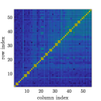
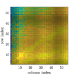
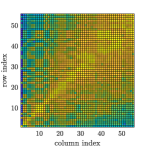
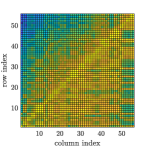
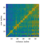
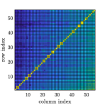
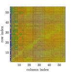
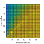
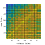
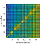
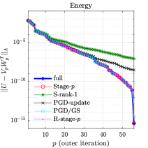
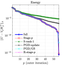
In the following sections, we compare the five AEM variants, Stage-p𝑝p (Algorithm 1), S-rank-111 (Algorithm 2), PGD-updated  (Algorithm 6), PGD/GS-updated  (Algorithm 7), and reduced stage-p𝑝p  (Algorithm 8). For orthonormalization in PGD-updated  (Algorithm 6) and reduced stage-p𝑝p  (Algorithm 8), we use Matlab’s qr function. For assessing performances, we explore two key aspects. The first is the accuracy of the computed solutions, which we assess by computing two error metrics: cosines of angles between the truth singular vectors and the columns of the computed factors (Section 4.2.1), and errors between the truth solution and the computed solution measured in three different norms (Section 4.2.2). The second aspect is timings and scalability (Section 4.2.3). As the assessment of the first aspect requires the ground truth solution of (56), which is computed using Matlab’s backslash operator, and its singular vectors, we choose small-sized problems in Sections 4.2.14.2.2. When making comparisons with the truth solution, we set the maximum number of outer iterations for all the AEM methods to be pmax=min(nx,nξ)=56subscript𝑝subscript𝑛𝑥subscript𝑛𝜉56p_{\max}=\min(n_{x},n_{\xi})=56. Larger problems are considered in Section 4.2.3, where scalability matters and finding the truth solution is impossible with the available resources.

[Uncaptioned image]
Refer to caption
(a) Stage-p𝑝p, VV~p𝖳superscript𝑉superscriptsubscript~𝑉𝑝𝖳V^{\ast}{}^{\mathsf{T}}\widetilde{V}_{p}
Refer to caption
(b) S-rank-111, VV~p𝖳superscript𝑉superscriptsubscript~𝑉𝑝𝖳V^{\ast}{}^{\mathsf{T}}\widetilde{V}_{p}
Refer to caption
(c) PGD-update, VV~p𝖳superscript𝑉superscriptsubscript~𝑉𝑝𝖳V^{\ast}{}^{\mathsf{T}}\widetilde{V}_{p}
Refer to caption
(d) PGD/GS, VV~p𝖳superscript𝑉superscriptsubscript~𝑉𝑝𝖳V^{\ast}{}^{\mathsf{T}}\widetilde{V}_{p}
Refer to caption
(e) R-stage-p𝑝p, VV~p𝖳superscript𝑉superscriptsubscript~𝑉𝑝𝖳V^{\ast}{}^{\mathsf{T}}\widetilde{V}_{p}
Figure 1: Cosines of angles (plotted in log\log scale) between the left singular vectors Vsuperscript𝑉V^{\ast} and V~psubscript~𝑉𝑝\widetilde{V}_{p}, and the right singular vectors Wsuperscript𝑊W^{\ast} and W~psubscript~𝑊𝑝\widetilde{W}_{p}, where V~psubscript~𝑉𝑝\widetilde{V}_{p} and W~psubscript~𝑊𝑝\widetilde{W}_{p} are computed using the Stage-p𝑝p and S-rank-111 AEM methods, and the EnhancedAEM methods with PGD-update, PGD/GS, and R-stage-p𝑝p enhancements.

  [Uncaptioned image] Refer to caption (f) Stage-p𝑝p, WW~p𝖳superscript𝑊superscriptsubscript~𝑊𝑝𝖳W^{\ast}{}^{\mathsf{T}}\widetilde{W}_{p} Refer to caption (g) S-rank-111, WW~p𝖳superscript𝑊superscriptsubscript~𝑊𝑝𝖳W^{\ast}{}^{\mathsf{T}}\widetilde{W}_{p}
Refer to caption (h) PGD-update, WW~p𝖳superscript𝑊superscriptsubscript~𝑊𝑝𝖳W^{\ast}{}^{\mathsf{T}}\widetilde{W}_{p} Refer to caption (i) PGD/GS, WW~p𝖳superscript𝑊superscriptsubscript~𝑊𝑝𝖳W^{\ast}{}^{\mathsf{T}}\widetilde{W}_{p} Refer to caption (j) R-stage-p𝑝p, WW~p𝖳superscript𝑊superscriptsubscript~𝑊𝑝𝖳W^{\ast}{}^{\mathsf{T}}\widetilde{W}_{p}

4.2.1 Relation to singular vectors

We begin by exploring how the factors in the approximate solutions constructed by each of the methods compare with the left and right singular vectors of the true solution matrix U𝑈U. This is important because (i) singular vectors represent the most effective choice with respect to the Frobenius norm for approximating a matrix U𝑈U. That is, the minimum error over all rank-p𝑝p approximations is UV~pΣpW~p𝖳Fsubscriptnorm𝑈subscript~𝑉𝑝subscriptΣ𝑝superscriptsubscript~𝑊𝑝𝖳F\|U-\widetilde{V}_{p}\Sigma_{p}\widetilde{W}_{p}^{\mathsf{T}}\|_{\text{F}}, where U=V~ΣW~𝖳𝑈~𝑉Σsuperscript~𝑊𝖳U=\widetilde{V}\Sigma\widetilde{W}^{\mathsf{T}} is the singular value decomposition [7], and (ii) in some applications such as collaborative filtering for recommendation systems, computing singular vectors accurately is very important for precise predictions [16, 17, 40]. For these tests, the diffusion coefficient is given by (57) with (μ,σ)=(1,.1)𝜇𝜎1.1(\mu,\sigma)=(1,.1) and c=2𝑐2c=2. We use a spatial discretization with grid level 4 (i.e., grid spacing 1241superscript24\frac{1}{2^{4}}, and nx=225subscript𝑛𝑥225n_{x}=225) and we truncate the expansion (57) at m=5𝑚5m=5. For the stochastic Galerkin approximation, we choose dtot=3subscript𝑑tot3d_{\text{tot}}=3 which gives nξ=56subscript𝑛𝜉56n_{\xi}=56.

For any approximation of the form (3), let V~psubscript~𝑉𝑝\widetilde{V}_{p} and W~psubscript~𝑊𝑝\widetilde{W}_{p} be normalized versions of the factors, i.e., each column of V~psubscript~𝑉𝑝\widetilde{V}_{p} and W~psubscript~𝑊𝑝\widetilde{W}_{p} is scaled to have unit norm. From the ground truth solution U𝑈U, the matrices Vsuperscript𝑉V^{\ast} and Wsuperscript𝑊W^{\ast} of left and right singular vectors are computed. The entries of VV~p𝖳superscript𝑉superscriptsubscript~𝑉𝑝𝖳V^{\ast}{}^{\mathsf{T}}\widetilde{V}_{p}, the cosines of the angles between the left singular vectors of the true solution and the left vectors defining the approximate solution, together with the analogous angles for the right vectors, WW~p𝖳superscript𝑊superscriptsubscript~𝑊𝑝𝖳W^{\ast}{}^{\mathsf{T}}\widetilde{W}_{p}, give insight into the quality of the approximate solution. Figures 1a and 1f and Figures 1b and 1g depict the cosines of the angles between the singular vectors and the columns of V~psubscript~𝑉𝑝\widetilde{V}_{p} and W~psubscript~𝑊𝑝\widetilde{W}_{p} computed using the Stage-p𝑝p AEM and S-rank-111 AEM methods discussed in Section 2. It can be seen from these results (in Figures 1a and 1f) that the Stage-p𝑝p AEM method does a good job of approximating the singular vectors of the solution. That is, the values of the diagonal entries are close to one and the values of the off-diagonal entries are close to zero. On the other hand, the S-rank-111 AEM method (see Figures 1b and 1g) is far less effective. The 2×2222\times 2 blocks on the diagonals in Figures 1a and 1f reflect the presence of equal singular values.

Figures 1c1e and 1h1j show analogous results for EnhancedAEM with PGD-update (Algorithm 6), PGD/GS (Algorithm 7), and R-stage-p𝑝p (Algorithm 8). Since we attempt to see each method’s best possible results without considering the computational costs, we set kmax=5subscript𝑘5k_{\max}=5 and nupdate=1subscript𝑛update1n_{\text{update}}=1 (i.e., enhancements are performed at every outer iteration) in Algorithm 3. For the same reason, we set PGD/GS to update all the solution pairs and, for R-stage-p𝑝p, we set τ=.001𝜏.001\tau=.001. With PGD-update, the spatial component gets reduced (i.e., we form K~i=V~p𝖳KiV~psubscript~𝐾𝑖superscriptsubscript~𝑉𝑝𝖳subscript𝐾𝑖subscript~𝑉𝑝\widetilde{K}_{i}=\widetilde{V}_{p}^{\mathsf{T}}K_{i}\widetilde{V}_{p}) and Wpsubscript𝑊𝑝W_{p} is updated. Figures 1c and 1h show that this computation improves the quality of the resulting factor Wpsubscript𝑊𝑝W_{p} (and Vpsubscript𝑉𝑝V_{p} as well) as approximate singular vectors, compared to those obtained with the S-rank-111 method. It is evident that PGD/GS further improves the quality of V~psubscript~𝑉𝑝\widetilde{V}_{p} and W~psubscript~𝑊𝑝\widetilde{W}_{p} (Figures 1d and 1i) as approximate singular vectors, and R-stage-p𝑝p is nearly as effective as the Stage-p𝑝p AEM approach (Figures 1e and 1j).

4.2.2 Assessment of solution accuracy

We now compare the convergence behavior of the variants of the AEM methods introduced in Sections 2 and 3. We use two different settings for the stochastic diffusion coefficient: [exp1] (μ,σ)=(1,.1)𝜇𝜎1.1(\mu,\sigma)=(1,.1), c=2𝑐2c=2 and [exp2] (μ,σ)=(1,.2)𝜇𝜎1.2(\mu,\sigma)=(1,.2), c=.5𝑐.5c=.5. We again truncate the series (57) at m=5𝑚5m=5 and, for the Legendre basis polynomials, we consider dtot=3subscript𝑑tot3d_{\text{tot}}=3 which gives nξ=56subscript𝑛𝜉56n_{\xi}=56. We deliberately keep the same value for m𝑚m and dtotsubscript𝑑totd_{\text{tot}} for both settings so that we can keep the dimensions of the problem the same and, thus, directly compare the behavior of each method in different problem settings. We also use the same parameters for the EnhancedAEM methods as before (i.e., kmax=5subscript𝑘5k_{\max}=5, nupdate=1subscript𝑛update1n_{\text{update}}=1, and τ=.001𝜏.001\tau=.001).

Refer to caption
(a) Energy norm - Exp1
Refer to caption
(b) Energy norm - Exp2
Figure 2: Solution errors measured in the energy norm

For each method, the approximate solution Upsubscript𝑈𝑝U_{p} is computed and we measure the accuracy compared to the reference solution U𝑈U. We did this using three different metrics: the energy norm error UUpAsubscriptnorm𝑈subscript𝑈𝑝𝐴\|U-U_{p}\|_{A}, the error in the Frobenius norm UUpFsubscriptnorm𝑈subscript𝑈𝑝F\|U-U_{p}\|_{\text{F}}, and the residual in the Frobenius norm B𝒜(Up)Fsubscriptnorm𝐵𝒜subscript𝑈𝑝F\|B-\mathcal{A}(U_{p})\|_{\text{F}}. Here, we only report the energy norm errors (in Figure 2), as behavior for the other two metrics is virtually identical. For comparison, a rank-p𝑝p reference solution (referred to as “full” in Figure 2) is also obtained directly from the first p𝑝p singular values and singular vectors of U𝑈U.

For both settings, as expected, the convergence behavior of the S-rank-111 AEM method is significantly worse than that of the rank-p𝑝p reference solution, whereas that of the Stage-p𝑝p AEM method is virtually the same as for the full direct solver. The EnhancedAEM method with PGD-update converges well until a certain level of accuracy is achieved, but it fails to achieve a high level of accuracy. In both experiments, the EnhancedAEM methods with PGD/GS and R-stage-p𝑝p are more effective than with the PGD-update. The accuracy that those two methods achieve is virtually the same as that of the Stage-p𝑝p AEM method and the full direct solver.

4.2.3 Computational timings

The above results do not account for computational costs; we now investigate timings under various experimental settings. This is important for large-scale applications, and so we now consider a finer spatial grid, with grid level 6 (i.e., grid spacing 1261superscript26\frac{1}{2^{6}}, and nx=3969subscript𝑛𝑥3969n_{x}=3969), as well as larger parameter spaces, with m={20,24}𝑚2024m=\{20,24\} (the number of random variables in (57)) and dtot=4subscript𝑑tot4d_{\text{tot}}=4, which results in nξ={10626,20475}subscript𝑛𝜉1062620475n_{\xi}=\{10626,20475\}. We use the same settings for the stochastic diffusion coefficient [exp1] (μ,σ)=(1,.1)𝜇𝜎1.1(\mu,\sigma)=(1,.1), c=2𝑐2c=2 and [exp2] (μ,σ)=(1,.2)𝜇𝜎1.2(\mu,\sigma)=(1,.2), c=.5𝑐.5c=.5. Again, we set m𝑚m and dtotsubscript𝑑totd_{\text{tot}} to be the same for both problems, as we want to keep the dimensions fixed so that we can make direct and fair comparisons.

Before we present these results, we summarize the systems of equations to be solved for each of the EnhancedAEM methods and the adjustable parameters that affect the performances of the methods.444The results of using the Stage-p𝑝p and S-rank-111 AEM methods are not reported because the Stage-p𝑝p AEM method is computationally too expensive and the S-rank-111 AEM method exhibits poor convergence behavior and, indeed, fails to satisfy the given convergence criterion. We first describe how we solve the systems arising at the p𝑝pth outer iteration when the condition for applying the enhancement is met, as well as the systems arising in RankOneCorrection (Algorithm 4). We use PCG to solve each system of equations using mean-based preconditioners [30], which are constructed using reduced versions of the matrices K0subscript𝐾0K_{0} and G0subscript𝐺0G_{0}, that are adapted to each method. For all systems, each PCG iteration requires matrix-vector products in the matricized form (see [2, 20, 23] for detailed matrix operations)

i=0m(Mx1K~i)X(Mξ1G~i)𝖳,superscriptsubscript𝑖0𝑚superscriptsubscript𝑀𝑥1subscript~𝐾𝑖𝑋superscriptsuperscriptsubscript𝑀𝜉1subscript~𝐺𝑖𝖳\sum_{i=0}^{m}(M_{x}^{-1}\widetilde{K}_{i})X(M_{\xi}^{-1}\widetilde{G}_{i})^{\mathsf{T}},

where X𝑋X is a quantity to be updated, K~isubscript~𝐾𝑖\widetilde{K}_{i} and G~isubscript~𝐺𝑖\widetilde{G}_{i} are reduced matrices, and Mxsubscript𝑀𝑥M_{x} and Mξsubscript𝑀𝜉M_{\xi} are the preconditioner factors. Table 1 summarizes each system matrix and preconditioner.555Note that, for PGD-update, one can always choose the smallest solution component to update. In practice, however, updating the Wpsubscript𝑊𝑝W_{p} component (i.e., reduction in {Ki}i=0msuperscriptsubscriptsubscript𝐾𝑖𝑖0𝑚\{K_{i}\}_{i=0}^{m}) always requires the smallest computational costs and, thus, we only report the result of updating Wpsubscript𝑊𝑝W_{p}.

Table 1: System matrices and preconditioners for each Enhancement procedure
Name X K~isubscript~𝐾𝑖\widetilde{K}_{i} G~isubscript~𝐺𝑖\widetilde{G}_{i} Mxsubscript𝑀𝑥M_{x} Mξsubscript𝑀𝜉M_{\xi} Eqs
S-rank-111 vpsubscript𝑣𝑝v_{p} Kisubscript𝐾𝑖K_{i} wp𝖳Giwpsuperscriptsubscript𝑤𝑝𝖳subscript𝐺𝑖subscript𝑤𝑝w_{p}^{\mathsf{T}}G_{i}w_{p} K0subscript𝐾0K_{0} 1 (17)
(Alg. 4) wp𝖳superscriptsubscript𝑤𝑝𝖳w_{p}^{\mathsf{T}} vp𝖳Kivpsuperscriptsubscript𝑣𝑝𝖳subscript𝐾𝑖subscript𝑣𝑝v_{p}^{\mathsf{T}}K_{i}v_{p} Gisubscript𝐺𝑖G_{i} 111 G0subscript𝐺0G_{0} (18)
PGD-update Vpsubscript𝑉𝑝V_{p} Kisubscript𝐾𝑖K_{i} W~p𝖳GiW~psuperscriptsubscript~𝑊𝑝𝖳subscript𝐺𝑖subscript~𝑊𝑝\widetilde{W}_{p}^{\mathsf{T}}G_{i}\widetilde{W}_{p} K0subscript𝐾0K_{0} W~p𝖳G0W~psuperscriptsubscript~𝑊𝑝𝖳subscript𝐺0subscript~𝑊𝑝\widetilde{W}_{p}^{\mathsf{T}}G_{0}\widetilde{W}_{p}
(Alg. 6) Wp𝖳superscriptsubscript𝑊𝑝𝖳W_{p}^{\mathsf{T}} V~p𝖳KiV~psuperscriptsubscript~𝑉𝑝𝖳subscript𝐾𝑖subscript~𝑉𝑝\widetilde{V}_{p}^{\mathsf{T}}K_{i}\widetilde{V}_{p} Gisubscript𝐺𝑖G_{i} V~p𝖳K0V~psuperscriptsubscript~𝑉𝑝𝖳subscript𝐾0subscript~𝑉𝑝\widetilde{V}_{p}^{\mathsf{T}}K_{0}\widetilde{V}_{p} G0subscript𝐺0G_{0} (48)
PGD/GS vlsubscript𝑣𝑙v_{l} Kisubscript𝐾𝑖K_{i} wl𝖳Giwlsuperscriptsubscript𝑤𝑙𝖳subscript𝐺𝑖subscript𝑤𝑙w_{l}^{\mathsf{T}}G_{i}w_{l} K0subscript𝐾0K_{0} 1 (49)
(Alg. 7) wl𝖳superscriptsubscript𝑤𝑙𝖳w_{l}^{\mathsf{T}} v¯l𝖳Kiv¯lsuperscriptsubscript¯𝑣𝑙𝖳subscript𝐾𝑖subscript¯𝑣𝑙\bar{v}_{l}^{\mathsf{T}}K_{i}\bar{v}_{l} Gisubscript𝐺𝑖G_{i} 1 G0subscript𝐺0G_{0} (50)
R-stage-p𝑝p V(p)subscript𝑉𝑝V_{\ell(p)} Kisubscript𝐾𝑖K_{i} W~(p)𝖳GiW~(p)superscriptsubscript~𝑊𝑝𝖳subscript𝐺𝑖subscript~𝑊𝑝\!\!\widetilde{W}_{\ell(p)}^{\mathsf{T}}G_{i}\widetilde{W}_{\ell(p)}\!\! K0subscript𝐾0K_{0} W~(p)𝖳G0W~(p)superscriptsubscript~𝑊𝑝𝖳subscript𝐺0subscript~𝑊𝑝\!\!\widetilde{W}_{\ell(p)}^{\mathsf{T}}G_{0}\widetilde{W}_{\ell(p)}\!\! (51)
(Alg. 8) W(p)𝖳superscriptsubscript𝑊𝑝𝖳W_{\ell(p)}^{\mathsf{T}} V~(p)𝖳KiV~(p)superscriptsubscript~𝑉𝑝𝖳subscript𝐾𝑖subscript~𝑉𝑝\widetilde{V}_{\ell(p)}^{\mathsf{T}}K_{i}\widetilde{V}_{\ell(p)} Gisubscript𝐺𝑖G_{i} V~(p)𝖳K0V~(p)superscriptsubscript~𝑉𝑝𝖳subscript𝐾0subscript~𝑉𝑝\widetilde{V}_{\ell(p)}^{\mathsf{T}}K_{0}\widetilde{V}_{\ell(p)} G0subscript𝐺0G_{0} (52)

Now, we discuss adjustable parameters. The EnhancedAEM methods (Algorithms 35) require parameters pmaxsubscript𝑝p_{\max}, kmaxsubscript𝑘k_{\max}, nupdatesubscript𝑛updaten_{\text{update}}, and ϵitalic-ϵ\epsilon. We set pmax=1000subscript𝑝1000p_{\max}=1000 to prevent excessive computations. We found that choosing kmax>2subscript𝑘2k_{\max}>2 results in negligible difference in accuracy, but requires extra computations and, thus, we use kmax={1,2}subscript𝑘12k_{\max}=\{1,2\}. For nupdatesubscript𝑛updaten_{\text{update}}, which determines how often the enhancement procedure is called, we vary nupdatesubscript𝑛updaten_{\text{update}} as {5,10,20,30}5102030\{5,10,20,30\}. Next, we use ϵitalic-ϵ\epsilon to check the convergence (as in Algorithm 5), and we vary ϵitalic-ϵ\epsilon as {1010,109,108,107}superscript1010superscript109superscript108superscript107\{10^{-10},10^{-9},10^{-8},10^{-7}\}. Finally, for PGD/GS and R-stage-p𝑝p, we empirically found that choosing τ>0.05𝜏0.05\tau>0.05 results in decreased accuracy in the approximate solution and, thus, we set τ=0.05𝜏0.05\tau=0.05.

Next, we set parameters for the PCG method. For all systems, the stopping criterion uses the relative residual in the Frobenius norm. We use two different tolerances: τbasissubscript𝜏basis\tau_{\text{basis}}{} for solving systems that arise in RankOneCorrection and PGD/GS, and τcoupledsubscript𝜏coupled\tau_{\text{coupled}}{} for solving systems that arise in PGD-update and R-stage-p𝑝p. We choose the values of τbasissubscript𝜏basis\tau_{\text{basis}}{} and τcoupledsubscript𝜏coupled\tau_{\text{coupled}}{} based on results of preliminary numerical experiments with the EnhancedAEM methods for (τbasis,τcoupled)={108,107,106,105}2subscript𝜏basissubscript𝜏coupledsuperscriptsuperscript108superscript107superscript106superscript1052(\tau_{\text{basis}}{},\tau_{\text{coupled}}{})=\{10^{-8},10^{-7},10^{-6},10^{-5}\}^{2}: (i) setting τbasis<105subscript𝜏basissuperscript105\tau_{\text{basis}}{}<10^{-5} does not result in improved accuracy of approximate solutions and, thus we set τbasis=105subscript𝜏basissuperscript105\tau_{\text{basis}}{}=10^{-5}, and (ii) for a given outer iteration tolerance ϵitalic-ϵ\epsilon, having too mild PCG tolerance τcoupled>102ϵsubscript𝜏coupledsuperscript102italic-ϵ\tau_{\text{coupled}}{}>10^{2}\epsilon results in poor performance and having stringent tolerance τcoupled<102ϵsubscript𝜏coupledsuperscript102italic-ϵ\tau_{\text{coupled}}{}<10^{2}\epsilon results in negligible difference in accuracy; thus, we use τcoupled=102ϵsubscript𝜏coupledsuperscript102italic-ϵ\tau_{\text{coupled}}{}=10^{2}\epsilon. Table 2 summarizes the parameters used for the experiments.

Table 2: Parameters used in the experiments for measuring timings
the maximum number of outer iterations pmax=1000subscript𝑝1000p_{\max}=1000
the maximum number of inner iterations kmax={1,2}subscript𝑘12k_{\max}=\{1,2\}
the frequency of the enhancement procedure nupdate={5,10,20,30}subscript𝑛update5102030n_{\text{update}}=\{5,10,20,30\}
the stopping tolerance for outer iterations ϵ={1010,109,108,107}italic-ϵsuperscript1010superscript109superscript108superscript107\epsilon\!=\!\{10^{-10},10^{-9},10^{-8},10^{-7}\}\!\!\!\!\!
PCG stopping tolerance for RankOneCorrection and PGD/GS τbasis=105subscript𝜏basissuperscript105\tau_{\text{basis}}{}=10^{-5}
PCG stopping tolerance for PGD-update and R-stage-p𝑝p τcoupled=102ϵsubscript𝜏coupledsuperscript102italic-ϵ\tau_{\text{coupled}}{}=10^{2}\epsilon
Refer to caption
Refer to caption
(a) m=20𝑚20m=20, [exp1]
Refer to caption
(b) m=24𝑚24m=24, [exp1]
Refer to caption
(c) m=20𝑚20m=20, [exp2]
Refer to caption
(d) m=24𝑚24m=24, [exp2]
Figure 3: Computational timings (in seconds) of three EnhancedAEM methods for varying kmaxsubscript𝑘k_{\max} and nupdatesubscript𝑛updaten_{\text{update}}. Timings of each method with each parameter set-up are averaged over 5 testing runs.

In Figure 3, we plot elapsed time (in seconds) against relative residual error for both [exp1] and [exp2]. Note that the relative residual is computed afterwards in a post-processing step. Recall that the stopping condition for the outer iteration (see Algorithm 5) is not based on the relative residual (as this is expensive to compute). The values of ϵitalic-ϵ\epsilon used for the stopping test for these results (see Algorithm 5) are shown in the figure. Note that for these experiments, the relative residual error is approximately three orders of magnitude larger than ϵitalic-ϵ\epsilon. Results obtained with the EnhancedAEM methods with PGD-update, PGD/GS, and R-stage-p𝑝p are marked in red, green, and blue, respectively, and each configuration of nupdatesubscript𝑛updaten_{\text{update}} and kmaxsubscript𝑘k_{\max} is marked with a different symbol. It can be seen from the figures that

  • the costs of R-stage-p𝑝p and PGD/GS are less sensitive to nupdatesubscript𝑛updaten_{\text{update}} and kmaxsubscript𝑘k_{\max} than those of PGD-update;

  • R-stage-p𝑝p is more efficient for smaller values of nupdatesubscript𝑛updaten_{\text{update}} whereas PGD/GS and PGD-update are better with larger nupdatesubscript𝑛updaten_{\text{update}};

  • for PGD-update and PGD/GS, relatively large nupdate>10subscript𝑛update10n_{\text{update}}>10 and kmax=2subscript𝑘2k_{\max}=2 results in better performances, and, for R-stage-p𝑝p, relatively small nupdate10subscript𝑛update10n_{\text{update}}\leq 10 and kmax=1subscript𝑘1k_{\max}=1 results in better performances.

Table 3 reports the number of outer iterations p𝑝p required to achieve the stopping tolerance ϵitalic-ϵ\epsilon for problems [exp1] and [exp2] when PGD-update, PGD/GS, and R-stage-pR-stage-𝑝\text{R-stage-}p are used. The benefit of using R-stage-p𝑝p becomes more pronounced as we seek highly accurate solutions with smaller ϵitalic-ϵ\epsilon. Our general observation is that among the three enhancement approaches, the R-stage-p method is less sensitive to choice of algorithm parameter inputs, scales better for larger problem sizes, and is the most effective of the three approaches.

Table 3: The number of outer iterations p𝑝p required to achieve the stopping tolerance ϵitalic-ϵ\epsilon for solving the problems [exp1] and [exp2] when PGD-update, PGD/GS, and R-stage-p𝑝p are used. The reported values of p𝑝p are computed by averaging values of p𝑝p obtained with the eight different combinations of nupdatesubscript𝑛updaten_{\text{update}} and kmaxsubscript𝑘k_{\max} shown in the legend of Figure 3.
[exp1]
m=20𝑚20m=20 m=24𝑚24m=24
PGD-update PGD/GS R-stage-p𝑝p PGD-update PGD/GS R-stage-p𝑝p
ϵ=107italic-ϵsuperscript107\epsilon=10^{-7} 163.8 160.4 152.9 184.9 177.8 173.0
ϵ=108italic-ϵsuperscript108\epsilon=10^{-8} 264.6 273.9 259.5 306.6 312.3 296.7
ϵ=109italic-ϵsuperscript109\epsilon=10^{-9} 356.3 363.7 340.1 415.0 421.5 397.3
ϵ=1010italic-ϵsuperscript1010\epsilon=10^{-10} 531.1 520.6 486.0 609.4 593.7 563.9
[exp2]
m=20𝑚20m=20 m=24𝑚24m=24
PGD-update PGD/GS R-stage-p𝑝p PGD-update PGD/GS R-stage-p𝑝p
ϵ=107italic-ϵsuperscript107\epsilon=10^{-7} 293.1 287.7 282.1 344.0 334.9 330.6
ϵ=108italic-ϵsuperscript108\epsilon=10^{-8} 414.6 422.7 397.7 492.8 506.7 478.3
ϵ=109italic-ϵsuperscript109\epsilon=10^{-9} 569.8 544.6 511.6 673.7 640.5 616.7
ϵ=1010italic-ϵsuperscript1010\epsilon=10^{-10} 821.6 716.4 677.1 933.1 848.1 810.1

We now briefly consider a second benchmark problem whose solution matrix has different rank characteristics and for which low-rank solvers ought to perform well.

4.3 Benchmark problem 2: fast decay coefficients

We define the random field a(x,ξ)𝑎𝑥𝜉a(x,\xi) as in (54) but now we choose ξiU(1,1)similar-tosubscript𝜉𝑖𝑈11\xi_{i}\sim U(-1,1) and the functions ai(x)subscript𝑎𝑖𝑥a_{i}(x) have coefficients that decay more rapidly than in the first benchmark problem. The details of this problem can be found in [8]. Specifically, the coefficients of the expansion are

a0=1,ai(x)=αicos(2πϱ1(i)x1)cos(2πϱ2(i)x2),i=1,2,,mformulae-sequencesubscript𝑎01formulae-sequencesubscript𝑎𝑖𝑥subscript𝛼𝑖2𝜋subscriptitalic-ϱ1𝑖subscript𝑥12𝜋subscriptitalic-ϱ2𝑖subscript𝑥2𝑖12𝑚a_{0}=1,\qquad a_{i}(x)=\alpha_{i}\cos(2\pi\varrho_{1}(i)x_{1})\cos(2\pi\varrho_{2}(i)x_{2}),\quad i=1,2,\ldots,m

where αi=α¯iσsubscript𝛼𝑖¯𝛼superscript𝑖𝜎\alpha_{i}=\bar{\alpha}i^{-\sigma} with σ>1𝜎1\sigma>1 and α¯¯𝛼\bar{\alpha} satisfies 0<α¯<1/ζ(σ)0¯𝛼1𝜁𝜎0<\bar{\alpha}<1/\zeta(\sigma), where ζ𝜁\zeta is the Riemann zeta function. Furthermore, ϱ1(i)=ik(i)(k(i)+1)/2subscriptitalic-ϱ1𝑖𝑖𝑘𝑖𝑘𝑖12\varrho_{1}(i)=i-k(i)(k(i)+1)/2 and ϱ2(i)=k(i)ϱ1(i)subscriptitalic-ϱ2𝑖𝑘𝑖subscriptitalic-ϱ1𝑖\varrho_{2}(i)=k(i)-\varrho_{1}(i) where k(i)=1/2+1/4+2i𝑘𝑖12142𝑖k(i)=\lfloor-1/2+\sqrt{1/4+2i}\rfloor. Our implementation is based on the Matlab software package S-IFISS [34]. In the following experiment, we choose σ=4𝜎4\sigma=4 and α¯=0.832¯𝛼0.832\bar{\alpha}=0.832. The parameter σ𝜎\sigma controls the rate of algebraic decay of the coefficients. The specific choice σ=4𝜎4\sigma=4 leads to fast decay and this causes the true solution matrix to have a lower rank than in the first benchmark problem.
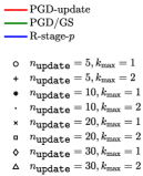
Refer to caption
Refer to caption
Figure 4: Computational timings (in seconds) of three EnhancedAEM methods for varying kmaxsubscript𝑘k_{\max} and nupdatesubscript𝑛updaten_{\text{update}}. Timings of each method with each parameter set-up are averaged over 5 testing runs.

We investigate computational timings of the EnhancedAEM methods with the same experimental settings used in Section 4.2.3. Here, we vary the stopping tolerance for the outer iterations as ϵ={109,108,107 106}italic-ϵsuperscript109superscript108superscript107superscript106\epsilon=\{10^{-9},10^{-8},10^{-7}\,10^{-6}\} and we choose the same values of nupdatesubscript𝑛updaten_{\text{update}} and kmaxsubscript𝑘k_{\max} as before. Figure 4 reports elapsed time (in seconds) against relative residual error. In nearly all cases, our observations agree with the findings in Figure 3. However, the impact of nupdatesubscript𝑛updaten_{\text{update}} is slightly less clear for these tests. The R-stage-p method is generally still less sensitive than the other two methods to the choices of nupdatesubscript𝑛updaten_{\text{update}} and kmaxsubscript𝑘k_{\max}, with one exception, indicated by the blue triangle marker, which is located to the far right in Figure 4. With nupdate=30subscript𝑛update30n_{\text{update}}=30, kmax=2subscript𝑘2k_{\max}=2, and ϵ=109italic-ϵsuperscript109\epsilon=10^{-9} (giving the right-most blue triangle), the R-stage-p𝑝p method does not meet the stopping criterion until p125𝑝125p\approx 125, which is larger than the value p90𝑝90p\approx 90 needed for the other choices of algorithm inputs. We attribute this to the large number of steps (30) between enhancements; in this case, the method fell just short of the stopping criterion after 90 steps. Finally, we report the number of outer iterations p𝑝p required to achieve the stopping tolerance ϵitalic-ϵ\epsilon in Table 4. As the true solution matrix has an intrinsic low-rank structure, the reported values of p𝑝p are much smaller than those shown in Table 3.

Table 4: The number of outer iterations p𝑝p required to achieve the stopping tolerance ϵitalic-ϵ\epsilon for solving the second benchmark problem when PGD-update, PGD/GS, and R-stage-p𝑝p are used. The reported values of p𝑝p are computed by averaging values of p𝑝p obtained with the eight different combinations of nupdatesubscript𝑛updaten_{\text{update}} and kmaxsubscript𝑘k_{\max} shown in the legend of Figure 4.
PGD-update PGD/GS R-stage-p𝑝p
ϵ=106italic-ϵsuperscript106\epsilon=10^{-6} 43.7 49.0 30.1
ϵ=107italic-ϵsuperscript107\epsilon=10^{-7} 58.3 68.3 41.4
ϵ=108italic-ϵsuperscript108\epsilon=10^{-8} 81.7 91.7 61.3
ϵ=109italic-ϵsuperscript109\epsilon=10^{-9} 130.9 121.6 91.6

4.4 Further Extensions

We also tested all the AEM methods on matrix equations obtained from stochastic Galerkin finite element discretizations of stochastic convection-diffusion problems [23, Section 5.2], where the randomness is in the diffusion coefficient as in Section 4.2. Although the energy norm cannot be defined for this problem because it has a non-symmetric operator, the same projection framework described herein can be applied to compute approximate solutions. Experiments (not reported here) were conducted similar to the ones in Sections 4.2.14.2.2. We observed that the proposed R-stage-p𝑝p method produces qualitatively better approximate factors Vpsubscript𝑉𝑝V_{p} and Wpsubscript𝑊𝑝W_{p}, as measured in the error metrics used in Sections 4.2.14.2.2, than the S-rank-111 AEM method and the other two EnhancedAEM methods.

5 Conclusions

In this study, we have investigated several variants of alternating minimization methods to compute low-rank solutions of linear systems that arise from stochastic Galerkin finite element discretizations of parameterized elliptic PDEs. Using a general formulation of alternating energy minimization methods derived from the well-known general projection method, our starting point was a variant of the stagewise ALS method, a technique for building rank-p𝑝p approximate solutions developed for matrix completion and matrix sensing. Our main contribution consists of a combination of this approach with so-called enhancement procedures of the type used for PGD methods [26, 27] in which rank-one approximate solutions are enhanced by adaptive use of higher-rank quantities that improve solution quality but limit costs by adaptively restricting the rank of updates. Experimental results demonstrate that the proposed PGD/GS and R-stage-p𝑝p methods produce accurate low-rank approximate solutions built from good approximations of the singular vectors of the matricized parameter-dependent solutions. Moreover, the results show that the R-stage-pR-stage-𝑝\text{R-stage-}p method scales better for larger problems, is less sensitive to algorithm inputs, and produces approximate solutions in the fastest times.

6 Acknowledgements

This paper describes objective technical results and analysis. Any subjective views or opinions that might be expressed in the paper do not necessarily represent the views of the U.S. Department of Energy or the United States Government. Sandia National Laboratories is a multimission laboratory managed and operated by National Technology and Engineering Solutions of Sandia, a wholly owned subsidiary of Honeywell International, for the U.S. Department of Energy’s National Nuclear Security Administration under contract DE-NA-0003525. This work was supported by the U.S. Department of Energy Office of Advanced Scientific Computing Research, Applied Mathematics program under award DE-SC0009301 and by the U.S. National Science Foundation under grant DMS1819115.

References

  • [1] I. Babuška, R. Tempone, and G. E. Zouraris, Galerkin finite element approximations of stochastic elliptic partial differential equations, SIAM Journal on Numerical Analysis, 42 (2004), pp. 800–825.
  • [2] J. Ballani and L. Grasedyck, A projection method to solve linear systems in tensor format, Numerical Linear Algebra with Applications, 20 (2013), pp. 27–43.
  • [3] S. Corveleyn, E. Rosseel, and S. Vandewalle, Iterative solvers for a spectral Galerkin approach to elliptic partial differential equations with fuzzy coefficients, SIAM Journal on Scientific Computing, 35 (2013), pp. S420–S444.
  • [4] S. V. Dolgov and D. V. Savostyanov, Alternating minimal energy methods for linear systems in higher dimensions, SIAM Journal on Scientific Computing, 36 (2014), pp. A2248–A2271.
  • [5] A. Doostan and G. Iaccarino, A least-squares approximation of partial differential equations with high-dimensional random inputs, Journal of Computational Physics, 228 (2009), pp. 4332–4345.
  • [6] A. Doostan, A. Validi, and G. Iaccarino, Non-intrusive low-rank separated approximation of high-dimensional stochastic models, Computer Methods in Applied Mechanics and Engineering, 263 (2013), pp. 42–55.
  • [7] C. Eckart and G. Young, The approximation of one matrix by another of lower rank, Psychometrika, 1 (1936), pp. 211–218.
  • [8] M. Eigel, M. Pfeffer, and R. Schneider, Adaptive stochastic Galerkin FEM with hierarchical tensor representations, Numerische Mathematik, 136 (2017), pp. 765–803.
  • [9] H. C. Elman and D. Furnival, Solving the stochastic steady-state diffusion problem using multigrid, IMA Journal of Numerical Analysis, (2007).
  • [10] H. C. Elman, A. Ramage, and D. J. Silvester, IFISS: A computational laboratory for investigating incompressible flow problems, SIAM Review, 56 (2014), pp. 261–273.
  • [11] R. G. Ghanem and P. D. Spanos, Stochastic Finite Elements: a Spectral Approach, Dover Publications, 2003.
  • [12] G. H. Golub and C. F. Van Loan, Matrix Computations, vol. 3, JHU Press, 2012.
  • [13] J. P. Haldar and D. Hernando, Rank-constrained solutions to linear matrix equations using powerfactorization, IEEE Signal Processing Letters, 16 (2009), pp. 584–587.
  • [14] M. Hardt, Understanding alternating minimization for matrix completion, in Foundations of Computer Science (FOCS), 2014 IEEE 55th Annual Symposium on, IEEE, 2014, pp. 651–660.
  • [15] P. Jain, R. Meka, and I. S. Dhillon, Guaranteed rank minimization via singular value projection, in Advances in Neural Information Processing Systems, 2010, pp. 937–945.
  • [16] P. Jain, P. Netrapalli, and S. Sanghavi, Low-rank matrix completion using alternating minimization, in Proceedings of the forty-fifth annual ACM Symposium on Theory of Computing, ACM, 2013, pp. 665–674.
  • [17] Y. Koren, R. Bell, and C. Volinsky, Matrix factorization techniques for recommender systems, Computer, (2009), pp. 30–37.
  • [18] D. Kressner and P. Sirković, Truncated low-rank methods for solving general linear matrix equations, Numerical Linear Algebra with Applications, 22 (2015), pp. 564–583.
  • [19] D. Kressner and C. Tobler, Krylov subspace methods for linear systems with tensor product structure, SIAM Journal on Matrix Analysis and Applications, 31 (2010), pp. 1688–1714.
  • [20] D. Kressner and C. Tobler, Low-rank tensor Krylov subspace methods for parametrized linear systems, SIAM Journal on Matrix Analysis and Applications, 32 (2011), pp. 1288–1316.
  • [21] O. P. Le Maître, O. M. Knio, B. J. Debusschere, H. N. Najm, and R. G. Ghanem, A multigrid solver for two-dimensional stochastic diffusion equations, Computer Methods in Applied Mechanics and Engineering, 192 (2003), pp. 4723–4744.
  • [22] K. Lee, K. Carlberg, and H. C. Elman, Stochastic least-squares Petrov–Galerkin method for parameterized linear systems, SIAM/ASA Journal on Uncertainty Quantification, 6 (2018), pp. 374–396.
  • [23] K. Lee and H. C. Elman, A preconditioned low-rank projection method with a rank-reduction scheme for stochastic partial differential equations, SIAM Journal on Scientific Computing, 39 (2017), pp. S828–S850.
  • [24] M. Loève, Probability Theory, Vol. II, vol. 46, Springer, 1978.
  • [25] G. J. Lord, C. E. Powell, and T. Shardlow, An Introduction to Computational Stochastic PDEs, Cambridge University Press, Cambridge, 2014.
  • [26] A. Nouy, A generalized spectral decomposition technique to solve a class of linear stochastic partial differential equations, Computer Methods in Applied Mechanics and Engineering, 196 (2007), pp. 4521–4537.
  • [27] A. Nouy, Proper generalized decompositions and separated representations for the numerical solution of high dimensional stochastic problems, Archives of Computational Methods in Engineering, 17 (2010), pp. 403–434.
  • [28] I. V. Oseledets, Tensor-train decomposition, SIAM Journal on Scientific Computing, 33 (2011), pp. 2295–2317.
  • [29] M. F. Pellissetti and R. G. Ghanem, Iterative solution of systems of linear equations arising in the context of stochastic finite elements, Advances in Engineering Software, 31 (2000), pp. 607–616.
  • [30] C. E. Powell and H. C. Elman, Block-diagonal preconditioning for spectral stochastic finite-element systems, IMA Journal of Numerical Analysis, 29 (2009), pp. 350–375.
  • [31] C. E. Powell, D. J. Silvester, and V. Simoncini, An efficient reduced basis solver for stochastic Galerkin matrix equations, SIAM Journal on Scientific Computing, 39 (2017), pp. A141–A163.
  • [32] B. Recht, M. Fazel, and P. A. Parrilo, Guaranteed minimum-rank solutions of linear matrix equations via nuclear norm minimization, SIAM review, 52 (2010), pp. 471–501.
  • [33] Y. Saad, Iterative Methods for Sparse Linear Systems, SIAM, 2003.
  • [34] D. J. Silvester, A. Bespalov, and C. E. Powell, S-IFISS, available online at http://www.manchester.ac.uk/ifiss/s-ifiss1.0.tar.gz.
  • [35] D. J. Silvester, H. C. Elman, and A. Ramage, Incompressible Flow and Iterative Solver Software (IFISS) version 3.5, September 2016. http://www.manchester.ac.uk/ifiss/.
  • [36] V. Simoncini, Computational methods for linear matrix equations, SIAM Review, 58 (2016), pp. 377–441.
  • [37] L. Tamellini, O. P. Le Maître, and A. Nouy, Model reduction based on proper generalized decomposition for the stochastic steady incompressible Navier–Stokes equations, SIAM Journal on Scientific Computing, 36 (2014), pp. A1089–A1117.
  • [38] D. Xiu, Numerical Methods for Stochastic Computations: a Spectral Method Approach, Princeton University Press, 2010.
  • [39] D. Xiu and G. E. Karniadakis, The Wiener-Askey polynomial chaos for stochastic differential equations, SIAM Journal on Scientific Computing, 24 (2002), pp. 619–644.
  • [40] Y. Zhou, D. Wilkinson, R. Schreiber, and R. Pan, Large-scale parallel collaborative filtering for the Netflix prize, in International conference on algorithmic applications in management, Springer, 2008, pp. 337–348.