A connection between the Ice-type model of Linus Pauling and the three-color problem

Abstract

The ice-type model proposed by Linus Pauling to explain its entropy at low temperatures is here approached in a didactic way. We first present a theoretically estimated low-temperature entropy and compare it with numerical results. Then, we consider the mapping between this model and the three-colour problem, i.e.,colouring a regular graph with coordination equal to 4 (a two-dimensional lattice) with three colours, for which we apply the transfer-matrix method to calculate all allowed configurations for two-dimensional square lattices of $N$ oxygen atoms ranging from 4 to 225. Finally, from a linear regression of the transfer matrix results, we obtain an estimate for the case $N\rightarrow\infty$ which is compared with the exact solution by Lieb.

I Introduction

Counting problems are part of our daily lives, normally disguised in the format of probability calculation. There is no way to estimate probabilities (at least within the Laplace definition) without enumerating all possibilities (the sample space), which is why lottery apportionment is frequently postponed to later weeks. In addition to challenging gamblers, this type of games often resists the cleverness and intelligence of mathematicians, statisticians, and physicists. This is what happened with the so-called ice-type model, the subject of this article. It can be summarized with a simple question: How many different ways can hydrogen bonds be arranged if water is frozen to $T=0$ K? In the nomenclature of thermodynamics, what is the residual entropy of the ice, i.e. $S=k_{B}\ln\Omega$? Here, $k_{B}$ is the Boltzmann constant, $\Omega$ is the number of accessible configurations to the system with $N$ oxygen atoms. This is not only a curiosity. Such problem appeared in 1933 when Giauque & Ashley Giauque measured the entropy of ice at low temperatures and found the molar entropy to be $s=0.82\pm 0.05\$cal/(mol K), remembering that $1$cal$\ \approx 4.18$ J. The molar entropy corresponds to the product of the Avogrado number ($N_{0}$) by the entropy per site, which is $S/N=k_{B}\frac{1}{N}\ln\Omega=k_{B}\ln\Omega^{1/N}$ or $k_{B}\ln W$, where $W=\Omega^{1/N}$.

It is important to note that the answer depends on the spatial dimension in which the H₂O molecules are inserted.

The first theoretical estimate for the residual entropy of ice was published in 1935 by Linus Pauling who obtained $s=0.805$ cal/(mol K) Pauling . This value is in good agreement with the experimental value, despite the several approximations used by Pauling. In Lieb’s own words Lieb , ”this calculation must be considered as one of the more fortunate applications of statistical mechanics to real substances”. Only in the 1960’s Nagle Nagle performed more precise numerical estimates for the entropy for a three-dimensional lattice and taking into account interaction among the vertices in a structure that simulates the ice and obtained $s=0.8145\pm 0.0002$ cal/(mol K). Both results are in complete agreement with the experimental estimate obtained by Giauque and Ashley Giauque .

Considering a two-dimensional version for the ice, Nagle obtained $s=$ $0.8580\pm 0.0013\$cal/(mol K) Nagle ; Nagle2 . Lieb Lieb obtained an exact solution for the problem in two dimensions ($s=0.856$ cal/(mol K)).

It is important to mention that the ice has a tetrahedral three-dimensional structure with oxygen atoms occupying the vertices. Thus, each oxygen atom is linked by hydrogen bonds to four other oxygen atoms. This means that the two-dimensional version of the model preserves a fundamental characteristic of the real structure which is the fact of each oxygen atom has four neighbours, with hydrogen atoms between them. Since each water molecule has only two hydrogen atoms, in the real structure, two of these hydrogen atoms must be in the nearest equilibrium position ($d=0.95$ Å) and the two other at the larger distance ($d=1.81$ Å), which belong to the neighbouring oxygen atoms. We shall come back to this subject and show that it corresponds to consider neutral molecules, giving rise to the well-known six-vertex model in Statistical Mechanics.

As the note added in proof of the paper by Lieb due to an observation of A. Lennard Lieb , this problem is equivalent, except by a factor 3, to discover how many ways exist to paint a square map using only 3 colours. A proper colouring of a map means that two neighbour countries cannot have the same colour, for if two countries have the same colour the border between them would disappear, i.e., the two countries would be merged into one.

In the next section we introduce the ice-type model and reproduce the calculation presented by Linus Pauling. In section III, we show the equivalence between this problem and the three-colouring map. In the same section, we also enumerate the acceptable configurations for small systems and present the numerical solution of the problem using a “brute force” method motivating our next section.

In section V we present an original numerical calculation developed for the colouring version of the problem which allows to proceed to the systems with $N=225$ atoms. In addition, after an extrapolation to the thermodynamic limit ($N\rightarrow\infty$), our numerical estimate is compared with the exact result by Lieb Lieb . Finally, we present some conclusions in section VI.

II The estimate of Linus Pauling

Since each hydrogen atom can be in two distinct positions, Pauling used an arrow to indicate if it is near (arrow comes in) or far (arrow exits of) each oxygen atom. The percentages of ions $H_{3}O^{+}$ and $OH^{-}$ are taken as zero which means that each oxygen atom (site in the lattice) must necessarily have 2 and only 2 hydrogen atoms next to it (two arrows arriving and two arrows departing from a site). The consequence is that from 16 possible types of vertices in Fig. 1, only $6$ (the first six vertices in that same plot, outlined in blue) satisfy the so-called “ice rules” introduced by Bernal and Fowler Bernal  in 1933 and improved by Pauling.

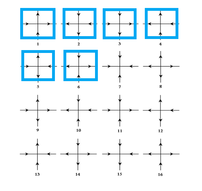
Figure 1: The sixteen possibilities of the vertex-types with only the six first vertices satisfying the ice rules, i.e., satisfying the conservation law where two and only two arrows are coming in (which means two and only two arrows coming out) (the allowed vertices outlined in blue).

This problem gave rise to the so called six-vertex model which was solved exactly in the 1960s. Returning to Pauling’s calculation, there is a fraction of $6/16$ allowed vertices in each site and the total number of configurations of the lattice (when one randomly chooses the direction of the $2N$ arrows starting from the $N$ oxygen atoms) is $2^{2N}$. Thus, assuming statistically independent sites (which is not true) and that in all $N$ vertices the ice rules are satisfied, we have

$$\begin{array}[]{lll}\Omega&\cong&2^{2N}(\frac{6}{16})^{N}\end{array}$$ (1)

or

$$W\cong\dfrac{3}{2},$$

which leads to an entropy per mol equal to

$$s=N_{0}k_{B}\ln W\cong R\ln(1.5)=0.805\ \text{cal}/(\text{mol\ }K),$$

where $N_{0}$ is the Avogadro number, $k_{B}$ is the Boltzmann constant and $\ R=N_{0}k_{B}=1.985$ cal$/($mol $K)$  is the universal gas constant.

III The language of colours

In this section we will show how the six-vertex model can be mapped onto the three colour problem.

Let us familiarize with the problem of colouring maps by analysing a small “world”with only 4 countries. There are 81 ways of painting the map with three colours, resulting from the operation with the product $(3\times 3\times 3\times 3)$ = $3^{4}$ since each country can be painted (in principle) with any of the three colours. However, many of these 81 ways do not satisfy the condition according to which two adjacent countries cannot be painted with the same colour. This condition destroys the independence between events, thus prohibiting the multiplication $3\times 3\times 3\times 3=3^{4}$ and drastically reducing the number of acceptable paintings. There is no simple reasoning to calculate this number because the events are not independent, but we may nevertheless solve the problem for a small number of countries. Let us consider that the countries are coloured with yellow (Y), green (G), and red (R). Fig. 2 shows the countries labelled as $P_{1},P_{2},P_{3}$ e $P_{4}$, starting from the upper left corner and rotating clockwise. The arrangement in Fig. 2 (a) does not satisfy the constraint as two neighbour countries are painted with the same colour ($P_{3}=P_{4}$). In contrast, the constraint is fulfilled in Fig 2 (b) where all neighbours are painted with distinct colours.

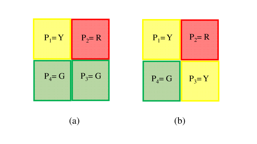
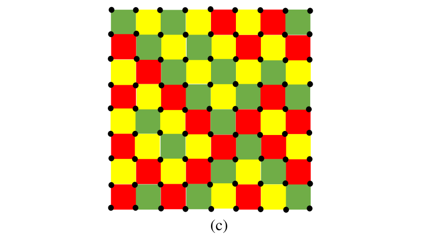
Figure 2: (a) Improper colouring (b) Proper Colouring. (c) Example of a proper colouring of a map with $8\times 8$ countries.

We can now enumerate the number of distinct paintings keeping in mind that after painting one of the countries, its neighbours can be coloured with one of the two remaining colours. For instance, if yellow is chosen to paint country $P_{1}$, country $P_{2}$ can only be painted with colours red or green. In addition, country $P_{4}$ has to satisfy the same constraint which means that choosing the colour of country $P_{1}$ one has $2+2=4$ ways to paint countries $P_{1}$, $P_{2}$ and $P_{4}$. For the remaining country $P_{3}$, there are the following alternatives: Either its two neighbours ($P_{2}$ and $P_{4}$) are painted with the same colour (both with the colour red or both with the colour green) or they are painted with different colours. In the first case country $P_{3}$ can be painted with colour yellow, the same colour of $P_{1}$, or with a remaining colour (G or R). Therefore, the two first possibilities are multiplied by 2, leading to 4 possible configurations. In the second case ($P_{2}$ and $P_{4}$ with different colours) there is no other way to paint $P_{3}$: it must be painted with the colour yellow (the same colour of $P_{1}$). The total number is then 6, the same found by Pauling for the number of vertices that satisfy the iced-type rules. However this is not yet the final result for the case of colours. We obtained 6 paintings by choosing yellow to paint $P_{1}$. There are 6 more possible colourings starting with Red for $P_{1}$ and another 6 by painting the first country with green. Therefore, the total number is $3\times 6=18$ different ways to colour a 4-country world with 3 colours.

But, why is this problem interesting to us? How does it work for larger worlds? In the next subsection we will show that the 3-colouring problem is equivalent to the six-vertex problem except by a multiplicative factor. It is important to notice that the colouring can contemplate more complex structures than simply maps (regular graphs) and using a different number of colours which is known graph-colouring. For the interested readers we strongly suggest read the Appendix I. In this appendix we present the problem in the light of the graph theory by showing extensions. In addition a report about analytical results related to the 3-colouring problem.

III.1 Mapping the six-vertex problem onto the three-colouring problem

Let us attribute the same three colours (yellow, green, and red) to countries in larger maps with the restriction that neighbouring countries cannot have the same colour. Fig 2 (c) shows a example of a proper colouring of a map with $8\times 8$ countries. .

We shall use a cyclical convention for the colours: Y follows G, G follows R, and R follows Y (YGRYGRYGR…). Every time that, rotating clockwise in relation to a perpendicular axis to the lattice plane, passing by the common point to the neighbouring 4 countries (the black points in Fig 2 (c)), and let us considering all worlds of the 4 countries in the $L\times L$ worlds.

Starting for example by convention from $P_{1}$ in each of these small worlds of the four countries, if we change from yellow to green (or from green to red or from red to yellow) the arrow in the boundary will be directed to the common point (blue arrow), while the changing from red to green (or from green to yellow or from yellow to red) it will be exiting from the common point (orange arrow), and this for both situations: horizontal and vertical boundaries.

This common point that resembles the position of oxygen atoms will always have two arrows in and two arrows out. Fig. 3 shows the six possible configurations of the arrows.

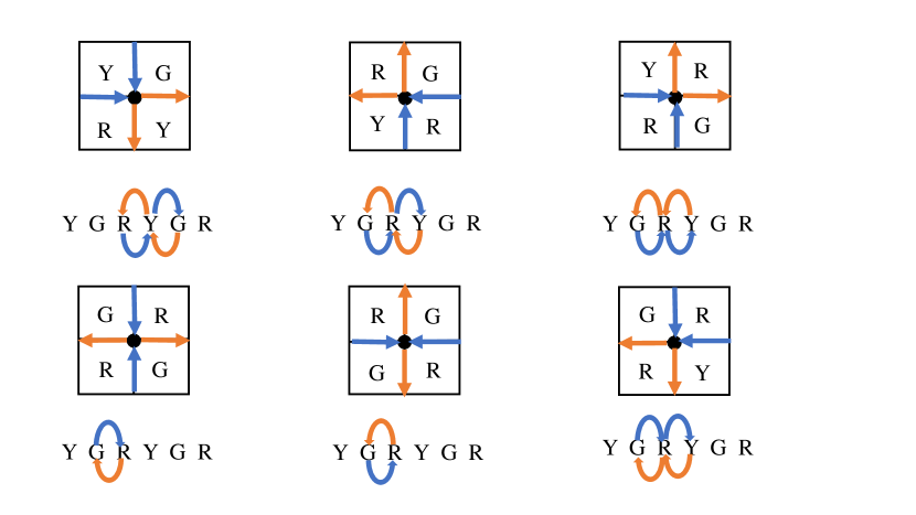
Figure 3: Examples of colourings of worlds with four countries translated to the possible 6 configurations of arrows. We start from P1 and rotate clockwise until P1 again following the cyclical convention established,considering blue (arrow in) and orange (arrow out). Any other configuration of colours is translated into one of these possible 6 configurations of arrows.

Let us consider the first colour configuration in that same figure 3. We start in $P_{1}$ with Y and $P_{2}$ with G, and following the clockwise orientation there is a blue vertical arrow pointing to the black point. From $P_{2}$ to $P_{3}$, one has G to Y, following the counter-clockwise direction, and thus there is an orange horizontal arrow out from the black point. From $P_{3}$ to $P_{4}\$ there is an orange vertical arrow out of the black point, and from $P_{4}$ to $P_{1}$ there is a blue horizontal arrow pointing to the black point. The other colourings in this translation only can lead to the one of possible arrow configurations represented in Fig. 3

It is reminded that each configuration of arrows corresponds to three possible colourings since there are three possible colours to start in $P_{1}$.

Thus we can write

$$\Omega_{\text{colours}}(N)=3W^{N}$$ (2)

and the factor 3 links the number of configurations of six-vertex problem to the three-colour problem.

However to solve this problem using a computer should be interesting to know if we can perform this calculation for larger values of $N$. In the next section we start this task first using an algorithm which calculates $\Omega_{\text{colours}}(N)$ using brute force (BF).

IV Computers and Brute Force: Preliminary Numerical Results

A table can be generated by showing the increasing of the number of possibilities $\Omega_{\text{colours}}(N)$ when the number of countries increases, which can be done by enumerating all possibilities of painting discarding the ones that do not satisfy the condition of the problem. A Fortran program (with Fortran 77), which can compiled in any Fortran compiler, with a few lines is sufficient to calculate $\Omega_{\text{colours}}(N)$ for a world with four countries (see Table: 1). This is carried out using “brute force”, i.e., checking all possible colourings in the map. In these programs we consider that G becomes 0, R becomes 1, and Y becomes 2.

	Program: Colouring a small world with 4 countries using exaustive enumeration (“Brute Force ”)
0	Integer $P_{1},P_{2},P_{3},P_{4},Icount$
1	$Icount=0$
2	Do $P_{1}=0,2$
3	Do $P_{2}=0,2$
4	Do $P_{3}=0,2$
5	Do $P_{4}=0,2$
6	If ($P_{1}$.ne.$P_{2}$.and.$P_{1}$.ne.$P_{4}$) then
7	If($P_{2}$.ne.$P_{3}$.and.$P_{4}$.ne.$P_{3}$) then
8	$\ \ \ \ \ \ \ \ \ \ \ \ \ \ \ \ \ \ \ \ \ \ \ \ \ \ \ \ \ Icount=Icount+1$
9	Endif
10	Endif
11	Enddo
12	Enddo
13	Enddo
14	Enddo
15	Write(*,*)${\acute{}}Number\ of\ configurations$ =${\acute{}}$,$\ Icount$
16	Stop
17	End

Table 1: A Brute Force algorithm

There is no increase in difficulty to replace a world of 4 countries to another with 9. The program will enumerate $3^{9}=\allowbreak 1.\,9683\times 10^{4}$ configurations for $9$ countries, using one of two alternatives: Free boundary conditions (FBC) or Periodic boundary conditions (PBC) in one of the directions to perform the counting. This was not important for 4 countries because in that case there was no difference between FBC and PBC. However, for $N=9$ countries this is not the case. For example, $P_{1}$ is neighbour to $P_{3}$, or $P_{7}$ is neighbour to $P_{9}$ with PBC but such neighbourhood relations are not considered for FBC, i.e., the red links in Fig. 4 are removed. Note, for instance, how the brute force algorithm for $N=9$ with PBC (Table 2) demands a lot more of ”brute force” compared to the case of $N=4$.

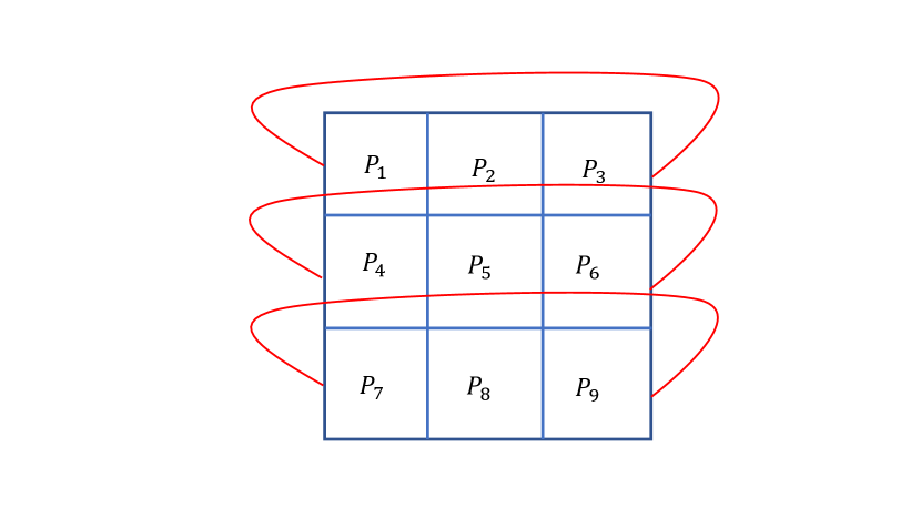
Figure 4: Configuration with $N=9$ countries. The red lines correspond to neighbourhood relations created for periodic boundary conditions. Such connections must be removed for free boundary conditions.

	Program: Colouring “Brute Force $N=9$”
0	Integer $P_{1},P_{2},P_{2},P_{3},P_{4},P_{5},P_{6},P_{7},P_{8},P_{9},Icount$
1	$Icount=0$
2	Do $P_{1}=0,2$
3	Do $P_{2}=0,2$
4	Do $P_{3}=0,2$
5	Do $P_{4}=0,2$
6	Do $P_{5}=0,2$
7	Do $P_{6}=0,2$
8	Do $P_{7}=0,2$
9	Do $P_{8}=0,2$
10	Do $P_{9}=0,2$
11	If ($P_{1}$.ne.$P_{2}$.and.$P_{1}$.ne.$P_{4}$) then
12	If ($P_{2}$.ne.$P_{3}$.and.$P_{2}$.ne.$P_{5}$) then
13	If ($P_{4}$.ne.$P_{5}$.and.$P_{4}$.ne.$P_{7}$) then
14	If($P_{5}$.ne.$P_{6}$.and.$P_{5}$.ne.$P_{8}$) then
15	If($P_{3}$.ne.$P_{6}$.and.$P_{6}$.ne.$P_{9}$.and.$P_{9}$.ne.$P_{8}$.and.$P_{8}.$ne.$P_{7}$) then
16	** Inclusion of the conditions for the PBC in one direction:
17	If($P_{1}$.ne.$P_{3}$.and.$P_{4}$.ne.$P_{6}$.and.$P_{7}$.ne.$P_{9}$) then
18	$\ \ \ \ \ \ \ \ \ \ \ \ \ \ \ \ \ \ \ \ \ \ \ \ \ \ \ \ \ \ \ \ \ \ \ \ \ \ \ \ \ \ \ \ \ \ \ \ \ \ \ \ \ \ \ \ \ \ \ \ \ \ \ \ \ \ \ \ \ \ \ \ \ \ \ \ \ \ \ \ \ \ Icount=Icount+1$
19	Endif
20	Endif
21	Endif
22	Endif
23	Endif
24	Endif
25	Enddo
26	Enddo
27	Enddo
28	Enddo
29	Enddo
30	Enddo
31	Enddo
32	Enddo
33	Enddo
34	Write(*,*)${\acute{}}Number\ of\ configurations$ =${\acute{}}$,$\ Icount$
35	Stop
36	End

Table 2: ”Brute Force” algorithm for N=9

For $N=16$ there are $3^{16}=\allowbreak 4.\,30467\,21\times 10^{7}$ colour configurations to select among them the acceptable colourings, which increase to $3^{25}$ or $8.\,47288\,60944\,3\times 10^{11}$ for $N=25$.

And how long would it take a personal computer to generate all those configurations? Well, it depends on the time it takes to generate each configuration. Actually, nowadays we have very fast personal computers and they can execute small operations in thousandths of billionths of a second. Technically, the computational performance is measured in FLOPS (floating-point operations per second) and so actually the computers operate in the scale of GIGAFLOPS and beyond.

For $N=25$, even thinking in GIGAFLOPS, the task is not easy, since it will be necessary at least $\Delta t\simeq$ $10^{12}$.$10^{-9}$ $=10^{3}\$seconds , or $10^{3}/(60)$ $\simeq$ $17$ minutes which is only a rough estimate. So the task gets more and more complicated even in faster computers. And there is not point in arguing that in faster computers will be possible to advance much more. For example, in order to enumerate the configurations of a map with $6$ $\times$ $6=36$ countries in the same time that we today perform the computation of the configurations for a map $5$ $\times$ $5$ it will be necessary to build a computer $170000$ faster than these which we are considering. Well, but the things are no so bad!

$N$	$\Omega_{\text{colours}}^{(FBC)}$	Time	$\Omega_{\text{colours}}^{(PBC)}$	Time
4	18	$<O(10^{-2})$	18	$<O(10^{-2})$
9	246	$<O(10^{-2})$	24	$<O(10^{-2})$
16	7812	$\approx\ 0.17$ sec	4626	$\approx 0.18\$sec
25	580986	$\approx 41$ min	38880	$\approx 39$ min

Table 3: Time spent to enumerate the acceptable configurations to paint a map with 9 countries by the ”brute force” method

We already have in hands some exact results from small systems using the “brute force” method (see Table 3). In that table, we show the execution of the algorithm using FBC and PBC. We also present the time required for the execution by using a processor Intel i7-8565 U for both situations. Sure, the time depends a lot on situations and we present the results of one execution only for an idea of the order of magnitude. Such times are impracticable since from $N=16$ to $N=25$, which are very small systems, the time changes from fraction of  seconds approximately to spent times about hours. Thus, it is mandatory to find a numerical alternative for working with larger systems which permits to us to do an extrapolation to the thermodynamic limit: $N\rightarrow\infty$. This will be performed in the next section.

V Elegant numerical results: The transfer-matrix method

For larger systems one has to resort a strategy very useful in Statistical Physics, which reduces a two-dimensional problem to a succession of one-dimensional problems. This approach is particularly useful for problems with cylindrical or toroidal geometry Barber , infinite in one of the directions. The first attempts to work with finite systems in two directions were made by Binder Binder . However, it was Creswick Creswick who obtained in 1995 the most efficient way to apply the technique to this geometry. Herein, we present this procedure in a system which is probably the most simple case where the technique can be applied, without requiring any prior knowledge of magnetic models and Statistical Mechanics. For that, we used functions of the programming language Fortran (similar functions exist in C language) and the task involves passing from one line (of countries) to the next. In the context of computer science this type of algorithm is known as greedy, since it discards the previously analysed instances. To apply this technique we also use PBC in one of the directions exactly as Creswick, which leads to a faster convergence at limit $N\rightarrow\infty$ when compared with FBC.

The calculation begins by choosing the possible colourings (configurations) for any line of countries. A country can be coloured with one of the three colours (from now on substituted by numbers $0,1$, and $2$) and two adjacent countries cannot have the same colour (the last country cannot have the colour of the first one due to PBC in the horizontal direction). Since $L$ is the width of the map there are

$$N_{\max}=(3-1)^{L}+(-1)^{L}(3-1)=2^{L}+2(-1)^{L}$$

possible different colourings to colour a line of countries, as shown in Eq. 5 in the Appendix A.

$N$	$\Omega_{\text{colours}}^{(PBC)}$	Time (secs)
4	$18$	$<O(10^{-2})$
9	$24$	$<O(10^{-2})$
16	$4626$	$<O(10^{-2})$
25	$38880$	$<O(10^{-2})$
36	$37284186$	$<O(10^{-2})$
49	$1886476032$	$<O(10^{-2})$
64	$9527634436194$	$\approx 0.016$
81	$2825260002442752$	$\approx 0.047$
100	$77048019386428981200$	$\approx 0.14$
121	$132046297983569476000000$	$\approx 0.66$
144	$19698820973096973600000000000$	$\approx 2.06$
169	$193554351965523488000000000000000$	$\approx 12$
196	$159147870862109172000000000000000000000$	$\approx 64$
225	$8920091695709351210000000000000000000000000$	$\approx 333$

Table 4: Results obtained with the transfer matrix method. The saving in processing times using this method when compared with BF method is notorious. One can run in a few minutes colourings with 225 countries. From $N=100$ onwards, the zeros are placed only to complete the power obtained in the numerical result since one has at most 18 significant digits in double precision.

There are $L$ loops and ($L/2+1$) decision commands (if’s) to discover the possible configurations during evolution. Next, we move to the second line that can also present only one of these acceptable configurations in the initial step. Among them, we need to discover which are the compatible colourings with each configuration of the first line, i.e., those with no two countries in the same position, coloured with the same colour. This operation can be performed associating each configuration of a line to an integer number, using a binary language. This integer has $2L$ bits since each country needs two bits to store its colour ($00$ corresponds to the colour $0$, $01$ corresponds to colour $1$, and $10$ to colour $2$). We then apply the operation exclusive $OR$ or simply $XOR$ ( $IEOR$ for Fortran compilers) to the two integers representing the configurations of the first and second lines. Since XOR (exclusive OR) works on all bits (see Fig. 5), then the result is $0$ if the bits are equal in the same position, and 1 if they are different. A double zero occurs only if one has the same bits occupying the same position in the lines, corresponding to two countries with the same colour.

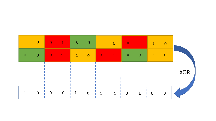
Figure 5: Exclusive OR (XOR) operation between two configurations. A double zero occurs only if one has the same bits occupying the same position in the lines.

Thus, $L$ decision commands (if’s) between bits of the integer resulting from operation IEOR(Line1,Line2) are enough to detect the existence of adjacent countries with the same colour. In this case, a configuration of the second line will not be compatible with the first line. After performing this selection, a comparison is made between the second and third lines and so on until the last line is considered, since the PBC condition does not apply in this direction. This is important to make the algorithm faster; it is thus greedy, i.e., information of past lines is discarded by using the subroutine Transfere accessed from the main algorithm (shown in Appendix II of this paper for $N=225$). The results with this algorithm in Table 4 are the same obtained by direct counting (BF) in the simpler cases ($N=9,16$ and $25$) but now it can be readily extended to $N=225$. It is then possible to perform an extrapolation to $N\rightarrow\infty$, shown in Fig. 6. According to Eq. 2 it is expected that $\ln\Omega_{\text{colours}}=\ln 3+N\ln W$, and a plot of $\ln\Omega_{\text{colours}}$ as function of $N$ suggests a linear behaviour with a slope numerically equal to $\ln W$, which is exactly observed in the Fig. 6.

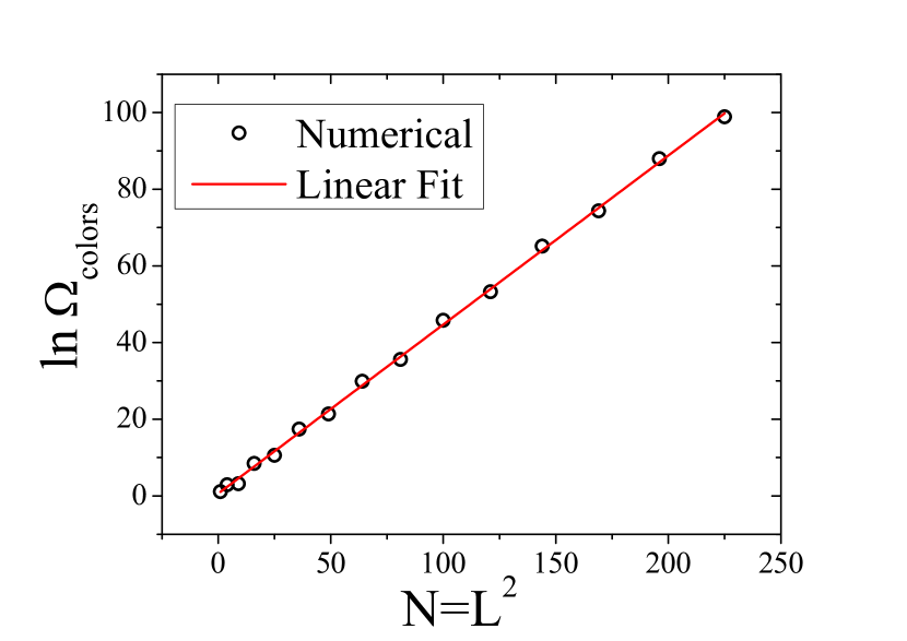
Figure 6: Plot of $\ln\Omega$ obtained by the transfer matrix method as function of $N$. It is expected that the slope of this curve gives an estimate to $\ln W$.

A linear fitting leads to $W_{num}=1.5421\pm 0.0054$ which must be compared with the result obtained by Lieb in 1967 Lieb :

$$W=(4/3)^{(3/2)}\approx 1.5396007.$$

Additional points about this result can be observed in Appendix I. After this problem treated by Lieb, actually based on the work of Lee and Yang LeeYang , other works involving six-vertex models were explored in the literature. The novelty about these problems is that vertices are not equally probable (they have no the same weight) since they represent energetically distinct situations. These models present phase transition even in one dimension when one changes the temperature Salinas since they do not obey the Mermin-Wagner theorem. But this is another history for other opportunity!

VI Conclusions

The problem of residual entropy of the ice was revisited by using a useful procedure in Statistical Mechanics. To employ this method, it was necessary to use a mapping of the ice-type model onto the problem of three colours.

The results with the transfer-matrix method indicate that even working with small systems and considering periodic boundary conditions in only one direction according to Creswick ideas, it is possible to obtain a good estimate by performing an extrapolation to the thermodynamic limit of the residual entropy. The use of the binary language in the representation of the configurations and the possibility of comparing two configurations, by using only simple operations with bits, is the other point that must be highlighted.

We call the attention of the reader, mainly that one who is interested in the Combinatorics and Number theory, for the exact result obtained by Lieb for $W=\lim_{N\rightarrow\infty}\Omega^{1/N}$ given by fraction of integers (4/3) raised to (3/2) with $\Omega$ corresponding to the number of the proper colourings of square lattices/maps with three colours. The colouring with more colours of the same square lattices, on the other hand, does not have an exact solution, only an upper and a lower bound are known in the thermodynamic limit as demonstrated by Biggs in 1977 Biggs77 .

Finally, the residual entropy of the ice is, no doubt, a interesting problem of the Physics and our main pedagogical contribution is to show that the transformation of the problem into the colouring map problem, makes possible an elegant numerical solution, accessible by undergraduate students and with only a basic knowledge in Mathematics and Computer Programming. In addition, more interested readers can go beyond considering more technical aspects in graph theory found in the first appendix, and that ones that desire to explore the computer codes by using transfer matrix method.

Appendix I: Understanding a little bit about graph theory and the problem of map colouring

Looking from a graph theory point of view, we can observe maps as a set of countries as vertices, while the borders between the countries representing edges linking these vertices. We can observe a map with four countries and its respective graph in the Figs. 7 (a) and 7 (b).

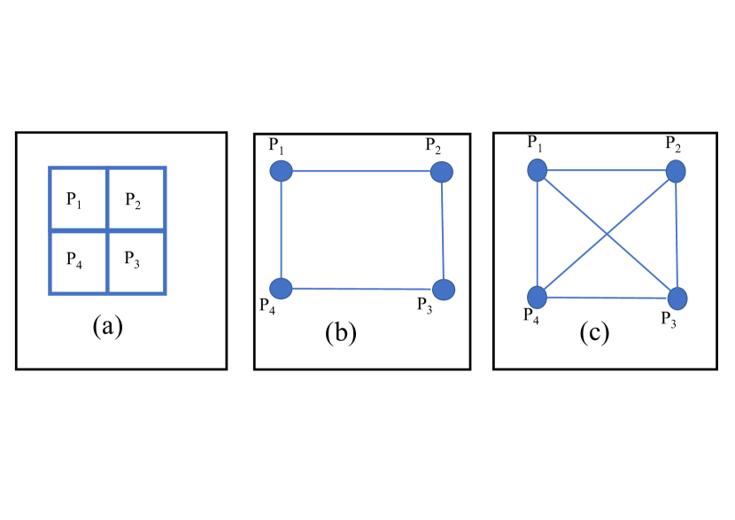
Figure 7: Plot (a) Map with four countries. Plot (b) Corresponding graph of the map represented in (a). Plot (c) This graph does not correspond to situation (a) since the country $P_{1}$ is not a neighbor of $P_{3}$, and $P_{2}$ is not a neighbour of $P_{4}$.

It is important to mention that the graph represented in Fig. 7 (c) does not correspond to the map observed in Fig. 7 (a) since the country $P_{1}$ is not a neighbour of $P_{3}$, and $P_{2}$ is not a neighbour of $P_{3}$. Since we studied as properly colouring with three colours a graph/map with four vertices/countries, the Graph theory is much more general and we can extend this for $x$ colours and even for more general graphs, which consists in a interesting and important illustration for readers that want to understand a little more about graph colouring.

In graph theory the number of ways to properly colour a graph with $x$ colours is so called the chromatic polynomial of this graph which is here denoted by $\phi(x)$, and you will see that for the graph 7 (b) it is a easy step since you have understood the case of 3 colours previously performed in this paper.

First there are only two possibilities: $P_{1}$ and $P_{3}$ have the same colour, or they have different colours. In the first case, one has $x$ ways to put the same colour simultaneously in $P_{1}$ and $P_{3}$ in this case you can colour $P_{2}$ with $x-1$ colours while $P_{4}$ one also has $x-1$ ways since they are not neighbours, so one has in this first case

$$\phi_{1}(x)=x(x-1)(x-1)=x(x-1)^{2}$$

On the other hand (second case) one has $P_{1}$ and $P_{3}$ painted with different colours. There are $x(x-1)$ ways to perform this task. For each of these possibilities, one can paint $P_{2}$ with $x-2$ colours and $P_{4}$ also with $x-2$ colours, resulting in this second case a total number of ways calculated by

$$\phi_{2}(x)=x(x-1)(x-2)(x-2)=x(x-1)(x-2)^{2}$$

Thus the total number of colouring the graph 7 (b) is

$$\begin{array}[]{lll}\phi(x)&=&\phi_{1}(x)+\phi_{2}(x)\\ &&\\ &=&x(x-1)^{2}+x(x-1)(x-2)^{2}\\ &&\\ &=&x(x-1)(x^{2}-3x+3)\end{array}$$ (3)

A fast test of this formulae is to perform the particular case $x=3$, and according to our previous calculations we must obtain $\phi(3)=18$, which is exactly the result previously obtained. Please see the graph in Fig. 7 (c). In this case we have all vertices connected to all vertices, and graphs that satisfy this condition are known as complete graphs and are denoted by $K_{n}$. The particular case of Fig. 7 (c) corresponds to $K_{4}$ (complete graph with $n=4$ vertices) and it must be observed that only the number of vertices define the graph since they have all possible edges (a total of $\binom{n}{2}$ edges for $K_{n}$). With some effort, one can observe that a proper colouring of this graph demands $x\geq n$ colours. Thus, the chromatic polynomial of the graph $K_{4}$ is easily calculated:

$$\phi_{K_{4}}(x)=x(x-1)(x-2)(x-3)$$

and the result can be extended for $K_{n}$, using the fundamental counting principle:

$$\phi_{K_{n}}(x)=x(x-1)(x-2)...(x-n+1)$$

Actually, these graphs are much more “sui generis” than we can imagine, since for example for $n\geq 5$ they have not a planar representation (or in simple words, a map representation), i.e., we cannot draw a planar representation of these graphs without necessarily having two or more edges intersecting. Let us better explain this point. For example, one observes that $K_{4}$ has a notorious planar representation (see Fig. 8 (a)), we are able to draw this graph as a map (in this case with 3 regions) or yet, without the edges intersecting (of course, unless the vertices themselves).

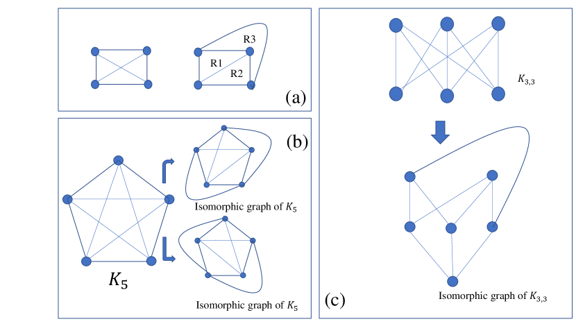
Figure 8: (a) $K_{4}$ is a planar graph (b) $K_{5}$ is not a planar graph. (c) $K_{3,3}$ is not also a planar graph. Both $K_{5}$ and $K_{3,3}$ are the small graphs non planar and represent fundamental structures for the graph theory.

On the other hand, we are not able to draw $K_{5}$ in a planar way. For example in Fig. 8 (b) we observe two attempts (two isomorphic graphs of $K_{5}$– i.e., roughly speaking are the same graph $K_{5}$ drawn in a different way). No one of them leads to a planar representation. The graph $K_{5}$ is a kind of “minimal non planar graph”. Other similar structure is the graph $K_{3,3}$ (complete bipartite graph on six vertices, three of which belonging a set only connect to each of the three belonging to the other set) that can be observed in Fig. 8 (c). Actually, any non-planar graph cannot have a subgraph which is a subdivision of the $K_{5}$ or $K_{3,3}$. But why the planarity is a important concept if we are talking about graph colouring? Because a fundamental theorem says that any planar graph can be properly coloured with a maximum of 4 colours. The theorem was demonstrated for the first time by 1976 by Kenneth Appel e Wolfgang Haken (see for example Four-Color ), by using an IBM 360, the first accepted proof by using a computer. For example $\phi_{K_{5}}(x)=x(x-1)(x-2)(x-3)(x-4)$. If we make $x=4$, $\phi_{K_{5}}(4)=0$ which corroborates the theorem, since $K_{5}$ is a non-planar graph. On the other hand $\phi_{K_{4}}(3)=0$, but $\phi_{K_{4}}(4)=24$ ways, which also corroborates the theorem since $K_{4}$ is a planar graph.

Let us go back to our world with four countries. As we saw, it is more complicated to colour this map than the graph $K_{4}$. We also can observe that a world with four countries is a particular case of colouring a disk of $n$ sectors/countries (Fig. 9 (a) ), where the Fig. 9 (b) is a graph representation of the this world where the countries are placed as disk sectors. This graph is known as a circular disk.

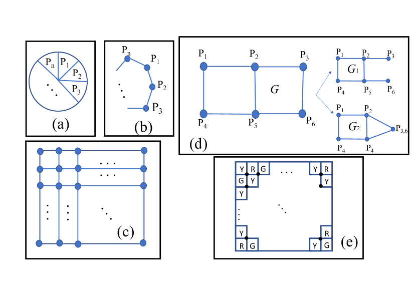
Figure 9: (a) Circular sector, (b) graph representation of a circular sector (c) A generalization of map with $N=L^{2}$ countries (a two-dimensional lattice) (d) Graph corresponding a world with 6 countries (e) A particular configuration of colours Y (yellow), G (green), and R (red) to the vertex of the lattice represented in (c) where the blue balls are changed by square cells (countries).

The idea is the same, for example, fixing two countries $P_{1}$ and $P_{3}$, or any couple of countries (non-adjacent sectors) separated by only a sector or neighbour a common sector (in this particular choice, $P_{2}$). In this situation we have two options, that these countries ($P_{1}$ and $P_{3}$) can be coloured with the same colour (situation I) or with two different colours (situation II). Denoting $\phi_{n}(x)$ the number of ways to properly colour this sector can be described by the recurrence relation

$$\phi_{n}(x)=(x-2)\phi_{n-1}(x)+(x-1)\phi_{n-2}(x)$$ (4)

which demands some explanation. In situation I, i.e., $P_{1}$ and $P_{3}$ have the same colour works as if these two sectors were merged in a same sector. Thus, for each colouring of the disk of $n-2$ sectors composed by the sector originated from the fusion of the sector $P_{1}$ with sector $P_{3}$ and by other all sectors $n-3$ sectors (except by sector $P_{2}$), one has $x-1$ ways to paint the sector $P_{2}$ which cannot have the same colour of $P_{1}$ neither $P_{3}$. On the other hand (situation II), we have that for each colouring of a disc with $n-1$ sectors composed by all sectors except by the sector $P_{2}$, and for each painting of this disk we have $x-2$ options to the sector $P_{2}$ which necessarily has a colour different of the colours attributed to neighbouring sectors $P_{1}$ and $P_{3}$, which justify the recurrence relation 4.

An interesting answer for this recurrence relation is $\varphi_{n}(x)=\alpha^{n}$, by direct substitution one has:

$$\alpha^{2}-(x-2)\alpha-(x-1)=0$$

that has two distinct roots: $\alpha_{1}=p-1$ and $\alpha_{2}=-1$, and a general solution is given by the linear combination: $\phi_{n}(x)=A(x-1)^{n}+B(-1)^{n}$. Such equation requires two initial conditions which we know. First a disk with two sectors has $\phi_{2}(x)=x(x-1)$ ways to be coloured, since the colour attributed to $P_{1}$ necessarily have a colour different of $P_{2}$. In a disk with 3 sectors, all of them are neighbours, thus similarly $\phi_{2}(x)=x(x-1)(x-2)$. So with these two initial conditions we can conclude that $A=1$ and $B=x-1$, which results in

$$\phi_{n}(x)=(x-1)^{n}+(-1)^{n}(x-1)$$ (5)

It is important to mention that such equation recovers the map with four countries (disk with four sectors) since $\phi_{4}(x)=(x-1)^{4}+(-1)^{4}(x-1)=x(x-1)(x^{2}-3x+3)$, exactly as we obtained in Eq. 3. After this tour across the graph theory and its connection with the colouring of the graphs, let us come back to the colouring of worlds with many countries. We already study the simple case of world with four countries described by Fig. 7 (a) and represented by Fig. 7 (b). In the case of many countries which is represented by the two-dimensional lattice (Fig. 9 (c) ), the colouring is not easy. We can start extending the world of four countries to six countries (Fig. 9 (d) ).  An important theorem in graph theory is the deletion-contraction theorem. This theorem says that for example choosing the edge between the countries $P_{1}$ and $P_{6}$ in the original graph ($G$), the chromatic polynomial of $G$ is the polynomial of the graph obtained by deletion of this edge ($G_{1}$) minus the polynomial of the graph obtained by contraction of this edge ($G_{2}$). To calculate $\phi_{G_{1}}(x)$, we can observe that it is obtained multiplying $\phi_{4}(x)$ times the ways of properly colouring the vertex $P_{3}$, which occurs in $x-1$ possible ways, times the ways of properly colouring the vertex $P_{6}$ which also occurs in $x-1$ possible ways, so:

$$\begin{array}[]{lll}\phi_{G_{1}}(x)&=&\phi_{4}(x).(x-1)(x-1)\\ &&\\ &=&x(x-1)^{3}(x^{2}-3x+3)\text{.}\end{array}$$

On the other hand, we must observe that the vertex $P_{3,6}$ has a stronger restriction, it can be coloured with colours different of $P_{2}$ and $P_{4}$ that always have different colours, thus

$$\begin{array}[]{lll}\phi_{G_{2}}(x)&=&\phi_{4}(x)(x-2)\\ &&\\ &=&x(x-1)(x-2)(x^{2}-3x+3)\end{array}$$

So, one has

$$\begin{array}[]{lll}\phi_{G}(x)&=&\phi_{G_{1}}(x)-\phi_{G_{2}}(x)\\ &&\\ &=&x(x-1)^{3}(x^{2}-3x+3)-x(x-1)(x-2)(x^{2}-3x+3)\\ &&\\ &=&x(x-1)(x^{2}-3x+3)^{2}\end{array}$$

With $x=3$ colours, we obtain $\phi_{G}(3)=54$ ways. In a more general case, one can attribute three colours (the same previous colours: Yellow, Green, and Red) to the vertices in the lattice (Fig. 9 (c) ) such that neighbouring vertices cannot have the same colour, exactly as countries in a map, by following our convention where vertices (little balls) correspond to cells (countries), as for example we can observe in Fig. 9 (e).We should naively imagine that recursively an expression for the lattice with $N=L^{2}$ countries should be obtained. But is is not true! Actually we have no an analytical expression for an arbitrary $N$.

In Biggs77 for example it is shown that for $N\rightarrow\infty$ upper and lower bounds are obtained:

$$\frac{1}{2}(x-2+\sqrt{x^{2}-4x+8})\geq\phi(x)\geq\frac{x^{2}-3x+3}{x-1}$$

However for $x=3$, both bounds are the golden ratio $\frac{1}{2}(1+\sqrt{5})$ and $3/2$. However Lieb in a brilliant work has obtained a exact result for $x=3$ at limit $N\rightarrow\infty$: $\phi_{\infty}(3)=(\frac{4}{3})^{3/2}$. But is $x=3$ an important case to us? Absolutely, since we can show that three-colouring problem is exactly the six-vertex problem (ice-type model) except by a multiplicative factor, which is exactly our original problem as we show in the the next subsection.

Appendix II: Transfer matrix algorithm for L=15 using PBC in one of the directions

1. Main algorithm

2. Subroutine

References

- (1) W. Giauque, M. Ashley, Phys. Rev. 43, 81 (1933)
- (2) L. Pauling, J. Am. Chem. Soc. 57, 2680 (1935)
- (3) E. H. Lieb, Phys. Rev. Lett. 18, 692 (1967), Phys. Rev. 162 , 162 (1967)
- (4) J. F. Nagle, Journal of Mathematical Physics 7, 1484 (1966)
- (5) It is important to mention that Nagle presented the estimate in his original work and not exactly an estimate for the entropy of the two-dimensional version of the ice-type model model. We take the liberty to present the estimate for based on this value considering that the uncertainty in was performed via error propagation: , once , where and are respectively the uncertainties in and , since cal/mol K.
- (6) J.D. Bernal, R. H. Fowler, J. Chem. Phys. 1, 515 (1933)
- (7) M. N. Barber in Phase Transitions and Critical Phenomena, vol.9, edited by Domb & Lebowitz, Academic Press, New York (1984)
- (8) K. Binder, Physica 62, 508 (1972)
- (9) R. J. Creswick, Phys. Rev. E 52, R5735 (1995)
- (10) C. N. Yang, T. D. Lee, Phys. Rev. 150, 321 (1966)
- (11) J. A. Plascak, S. R. A. Salinas, Rev. Bras. de Ensino de Fis. 10, 173 (1980)
- (12) N. Biggs, Bull. London Math. Soc. 9, 54 (1977)
- (13) K. Appel, W. Haken, The Four-Color Problem. In: Steen L.A. (eds) Mathematics Today Twelve Informal Essays. Springer, New York, NY (1978)