Shaken and stirred: When Bond meets Suess-de Vries and Gnevyshev-Ohl

1 Introduction

Thanks to the seminal work of Gerard Bond and his collaborators, we now have overwhelming evidence that a significant component of sub-Milankovich climate variability occurs in certain 1-3-kyears “cycles” of abrupt changes of the North Atlantic’s surface hydrography (Bond et al., 1997, 1999), and that those Bond events are closely related to corresponding variations in solar output, evidenced by measurements of the cosmogenic radionuclides ¹⁴C and ¹⁰Be (Bond et al., 2001). While originally identified for the Holocene (Bond et al., 1997) from certain ice drift proxies (in particular volcanic glass from Iceland and hematite-stained grains from East Greenland, found in deep-see sediments), many similar events were later revealed by Bond et al. (1999) in the last glacial period, too. Viewed from this angle, the little ice age, comprising in particular the Spörer and Maunder grand minima, appears just as the latest link in the chain of Bond events, and the temperature increase since the end of the Dalton minimum as a rebound from those frosty times.

In solar physics, similar variations with time scales of 1-3 kyears are usually discussed under the notion Eddy cycle and Hallstadt cycle (Steinhilber et al., 2012; Abreu et al., 2012; Soon et al., 2014; Scafetta et al., 2016; Usoskin et al., 2016). Yet, some caution seems to be appropriate when stretching the very concept of “cycles” from the decadal (Schwabe, Hale) to the millennial time scale, in particular when the underlying ¹⁴C and ¹⁰Be data bases have typical durations of only 10 kyears, or just slightly longer (Kudryavtsev and Dergachev, 2020). To gain more insight into the statistics of those “cycles”, we make here the plausible assumption that the established link between solar activity and Bond events, with correlation coefficients of around 0.5 during the Holocene (Bond et al., 2001), extends also to the last glacial. With this proviso, we re-plot in Figure fig:bond_and_sim(a) the data of time separations (or waiting times) between the 54 Bond events as identified over the last 80 kyears, which we have drawn from Figure 6(c) of Bond et al. (1999). What we observe then is a broad range of time separations between 600 years and 2600 years, with a mean value of 1469 years and a standard deviation of 514 years, according to Bond et al. (1999). However, when focusing only on the first eight time separations in the Holocene, located chiefly around 1500 years, 2400 years and 600 years, it comes as no surprise to find similar periods in Fourier or wavelet analyses (Mayewski et al., 1997; Dima and Lohmann, 2009; Soon et al., 2014). Special attention on the mean 1470-years cycle, and even speculations about its origin from a coincidence of 17 Gleissberg and 7 Suess-de Vries cycles (Braun et al., 2005), seem to be justified in this case.

If, on the contrary, we consider the entire series of Bond events over 80 kyears, we get the same impression as Usoskin et al. (2007) who had argued that the “occurrence of grand minima/maxima is driven not by long-term cyclic variability, but by a stochastic/chaotic process.” More quantitatively, the random walk character of this series is analyzed in Figure fig:bond_and_sim(b) which shows Dicke’s ratio $\sum_{i}^{N}r_{i}^{2}/\sum_{i}(r_{i}-r_{i-1})^{2}$ between the mean square of the residuals $r_{i}$ (i.e., the distances between the actual Bond events and hypothetical events according to a linear fit to the series) to the mean square of the differences $r_{i}-r_{i-1}$ between two consecutive residuals (Dicke, 1978). Obviously, Dicke’s ratio for $N$ Bond events taken into account roughly approaches the theoretical random walk dependence $(N+1)(N^{2}-1)/(3(5N^{2}+6N-3))$, with its limit $N/15$, while significantly deviating from the corresponding dependence $(N^{2}-1)/(2(N^{2}+2N+3))$ for a clocked process, with its limit $1/2$, as it had been confirmed previously for the Schwabe cycle (Stefani, Giesecke and Weier, 2019).

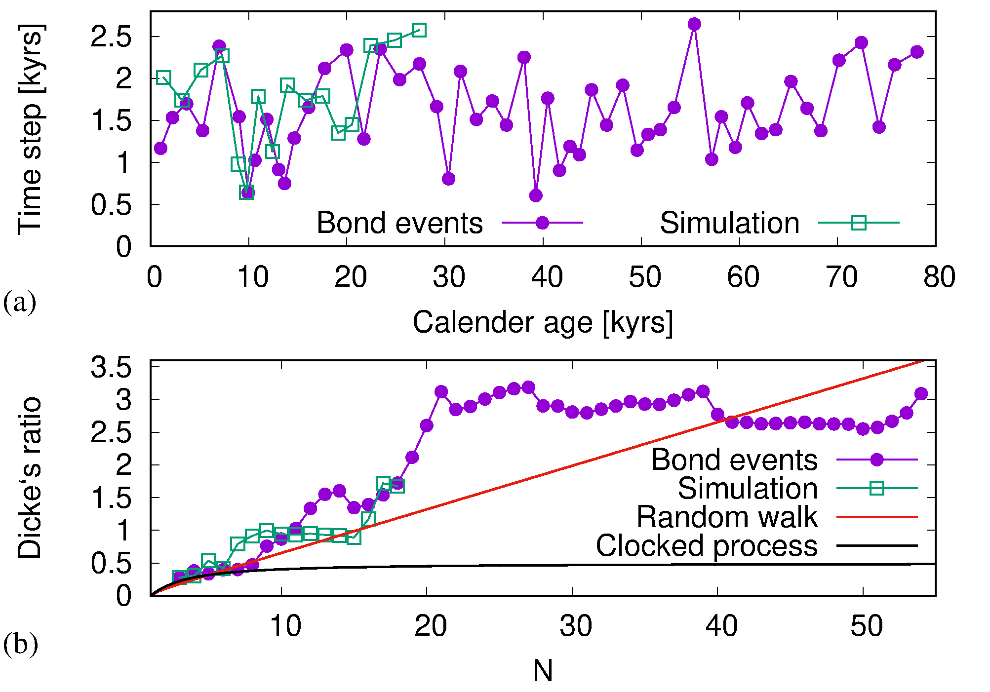
Figure 1.: (a) Violet full dots are time separations of the Bond events for the last 80 kyears, as inferred from Figure 6(c) of Bond et al. (1999) for the data of the deep-sea sediment core VM23-81. Green empty squares denote the corresponding time separations of numerically simulated “Bond events” for the parameters $\omega_{0}=10000$, $\alpha^{c}_{0}=15$, $\alpha^{p}_{0}=50$ $q^{p}_{\alpha}=0.2$, $q^{c}_{\alpha}=0.8$, $D=0.05$ and $\kappa(t)=0.6+0.2m(t)$). (b) Dependence of Dicke’s ratio on $N$ for the two time series from (a), together with the theoretical curves for a random walk and a clocked process. Note that the horizontal positions of the individual points slightly differ between (a) and (b) since the abscissa in (a) shows the centre point for the time separation, while the abscissa in (b) indicates the number of Bond events taken into account. fig:bond˙and˙sim

Figure fig:bond_and_sim(a) is complemented by another curve of 16 time separations (restricted to an interval of 30 kyears), as it will come out of our numerical model to be described further below. Suffice it to say here that the average of the waiting times, and their broad distribution, are quite similar to those of the 54 real Bond events, and that Dicke’s ratio points also in direction of a random walk process, although the statistical significance of those mere 17 numerical “Bond events” is certainly not satisfactory.

In this paper we will try to give a relatively simple and self-consistent answer to the questions of how such an intermittent and random walk like behaviour comes about, and how it can be related to the much clearer periodicities of the Hale, the Suess-de Vries, and the Gleissberg cycle(s). For this purpose, we will start from a rather conventional $\alpha-\Omega$-dynamo model in form of a simple 1D PDE system (with co-latitude as the only spatial variable), to allow for very long simulations of appr. 30 kyears. With the source terms $\alpha$ and $\Omega$ appropriately chosen, this dynamo develops typical oscillation periods of 20-30 years. After enhancing these internal “stirring” terms of the dynamo by two external “shaking” terms with the specific periods 11.07 years and 19.86 years (both being related to planetary motions), we will end up with a more or less complete reproduction of the most relevant temporal features of the solar dynamo. But beforehand, we have to clarify the origin of these two external “shaking” terms, and how their use in a solar dynamo model can be justified.

We start with the 11.07-years period. Although the similarity of the Schwabe cycle and the spring-tide period of the Venus–Earth–Jupiter (VEJ) system has been known for a long time (Bollinger, 1952; Takahashi, 1968; Wood, 1972; Condon and Schmidt, 1975), the precise correspondence of these two 11.07-years periodicities was recognized only recently by Hung (2007); Scafetta (2012); Wilson (2013); Okhlopkov (2014, 2016). According to Scafetta (2012), this period, corresponding to 4043 days, results from the resonance condition

$$P_{\rm VEJ} = \frac{1}{2}\left[\frac{3}{P_{\rm V}}-\frac{5}{P_{\rm E}}+\frac{2}{P_{\rm J}}\right]^{-1}$$ (1)

for the period of VEJ alignments, with the sidereal periods $P_{\rm V}=224.701$ days, $P_{\rm E}=365.256$ days, and $P_{\rm J}=44332.589$ days for Venus, Earth and Jupiter, respectively.

Quite often, the action of planetary tidal forces on the Sun is discarded in view of the tiny acceleration in the order of $10^{-10}$ ms^-2 (De Jager and Versteegh, 2005; Callebaut, de Jager, and Duhau, 2012), leading to a negligible tidal height $h_{\rm tidal}\approx GmR^{2}_{\rm tacho}/(g_{\rm tacho}d^{3})$ in the order of 1 mm ($m$ is the planet’s mass and $d$ its distance to the Sun). One should note, however, that this tidal height translates (by virtue of the virial theorem) into a non-negligible tidal flow velocity of $v\sim(2g_{\rm tacho}h_{\rm tidal})^{1/2}\approx 1$ m/s, when taking into account the huge gravity at the tachocline of $g_{\rm tacho}\approx 500$ m/s² (Öpik, 1972). But even then it is hard to conceptualize how tidal forces could influence the solar dynamo without employing any sort of amplification mechanism. One candidate for such a mechanism was discussed by Wolff and Patrone (2010); Scafetta (2012) who speculated that planetary forces might affect the nuclear burning rate deep in the solar core and that this effect would be promptly felt at the tachocline via the resulting change in g-mode oscillations. While this sounds highly speculative, we mention here a pertinent observation by Kotov and Haneychuk (2020) regarding a possible influence of Jupiter’s synodic cycle on the (still controversially discussed) 160 min oscillation of the Sun’s radius.

An entire suite of most interesting synchronization models was corroborated by Wilson (2013). First, the 11.07-years periodicity was explained in terms of a VEJ tidal-torque model, in which Jupiter plays a distinguished role by exerting a torque upon the periodically forming Venus-Earth tidal bulges. Second, a gear effect was invoked to modulate the changes in the rotation rates (as driven by the tidal-torque effect) by the 19.86-year periodic Saturn-Jupiter quadratures, leading ultimately to a long-term modulation with 193-year period (which will play a key role further below). Further derivations of a 208-years Suess-de Vries cycle, a 1156-years Eddy cycle, and a 2302-years Hallstatt cycle can also be found in this highly instructive and recommendable paper.

In Wilson (2013) and in the earlier model of Zaqarashvili (1997), the synchronization of the solar cycle was essentially based on some variation of the rotation rate in the tachocline and/or the convective layers of the Sun. This leads to the questions: how can the solar dynamo be synchronized by such a weak variation of $\Omega$? Both from our above estimation of the tidal effect on the velocity, as well as from the helioseismological measurements (Howe, 2009), we can infer that the variation of the $\Omega$ effect is certainly not larger than 1 per cent, and very likely much smaller, since a significant portion of the $\Omega$ variation can also be attributed to the back-reaction of the self-excited field on the flow (Proctor, 2007). If such a minor change is not sufficient to entrain the entire solar dynamo, can we perhaps take resort to the idea of Abreu et al. (2012) who emphasized that the maximum field strength of flux tubes (which can be stored prior to eruption) is very sensitive to small perturbations by gravitational, tidal and, as we add here, centrifugal forces due to changes of $\Omega$? Although our preliminary efforts (Stefani et al., 2018) to implement synchronization mechanisms of this sort into a Babcock-Leighton type dynamo model with time delay (Wilmot-Smith et al., 2006), either via a direct 11-07-years variation of the $\Omega$ effect or a corresponding variation of the rise condition for flux tubes, have not been very promising so far, we do not exclude that greater success may result from future investigations.

Still another avenue for synchronization was opened by Weber et al. (2015); Stefani et al. (2016), who recognized that the intrinsic helicity oscillations of the current-driven, kink-type Tayler instability (Tayler, 1973; Pitts and Tayler, 1985; Seilmayer et al., 2012; Weber et al., 2013), characterized by an azimuthal wavenumber $m=1$, can be entrained by a tide-like ($m=2$) perturbation, without (or barely) changing the energy content of the $m=1$ mode. This idea of an “energy-efficient” mechanism of helicity synchronization was then first incorporated into a simple ODE solar dynamo model (Stefani et al., 2016, 2017, 2018), and later into a 1D PDE system with the co-latitude as the only spatial variable (Stefani, Giesecke and Weier, 2019). From the 11.07-years tidal entrainment of the helicity, and the $\alpha$-effect associated with it, these models produced dipolar fields with an oscillatory 22.14-years Hale cycle, although in some parameter regions quadrupolar and hemispherical fields were observed, too. For the somewhat academic case of a purely 11.07-years periodic $\alpha$-effect we proved the existence of a massively nonlinear dynamo of the Tayler-Spruit type (Spruit, 2002; Rüdiger and Schultz, 2020), whereas for a more realistic hybrid dynamo, comprising both an externally “shaken” and an internally “stirred” $\alpha$-term, synchronization was accomplished by parametric resonance.

We would like to point out that meanwhile the empirical evidence for an 11.07-years synchronization is quite impressive, though not accepted (or not even recognized) throughout the solar dynamo community. Not only have the cycle minima from the last 1000 years turned out to be very close to a clocked-process with 11.07-years periodicity (Stefani, Giesecke and Weier, 2019), but various algae growth data from a 1000-years period in the early Holocene have also shown a phase coherent cycle with basically the same period (Vos et al., 2004).

As longer-term cycles are concerned, it was recently confirmed (Stefani et al., 2020a) that the modulation period of the duration of the Schwabe cycles, as inferred from Schove’s maxima data (Schove, 1983), is close to 200 years, a number which is consistent with previous results for the Suess-de Vries cycle relying on historic sunspot observations (Ma and Vaquero, 2020), ¹⁰Be and ¹⁴C data (Muscheler et al., 2007), and various climate related data (Lüdecke, Weiss and Hempelmann, 2015). It was not least the relative sharpness of that Suess-de Vries cycle which had motivated many authors (Jose, 1965; Fairbridge and Shirley, 1987; Charvatova, 1997; Landscheidt, 1999; Abreu et al., 2012; Wolff and Patrone, 2010; McCracken, Beer and Steinhilber, 2014; Cionco and Soon, 2015; Scafetta et al., 2016) to search for a link between the solar dynamo and planetary forcings with correspondingly long periods.

Yet, when entering this playing field one can hardly avoid the question why not to consider, first and foremost, the strongest of all planetary influences on the Sun’s motion, namely the 19.86-years synodic cycle of Jupiter and Saturn. This cycle governs the orbit of the Sun around the barycenter of the planetary system, comprising vast deflections in the order of the Sun’s diameter and velocities of up to 15 m/s (Sharp, 2013; Cionco and Pavlov, 2018). Superposed on that period are minor wiggles stemming mainly from the orbits of Uranus and Neptun, which ultimately leads to a rather complicated motion with another 172-years periodicity, sometimes called “Jose cycle” (Jose, 1965; Charvatova, 1997; Landscheidt, 1999; Sharp, 2013). Still, it is the dominant 19.86-years cycle which has the capacity to produce, in concert with the 22.14-years Hale cycle, a beat period of $19.86\times 22.14/(22.14-19.86)=193$  years, as worked out in the above mentioned paper by Wilson (2013) and also by Solheim (2013). This 193-years period is suspiciously close to the Suess-de Vries cycle. Assuming an appropriate, though not yet well understood, coupling effect of the Sun’s orbital motion into some change of the stratification of the tachocline, this beat period was numerically found to produce a 193-years modulation of the North-South asymmetry of the dynamo field (Stefani et al., 2020a).

This sequel to Stefani, Giesecke and Weier (2019); Stefani et al. (2020a) is structured as follows: in Section 2 we recapitulate our 1D solar dynamo code, and motivate the choice and structure of its main ingredients, such as the $\Omega$ effect, two parts of the $\alpha$-effect, and the time variation of the loss parameter $\kappa$. The results of our simulations over 30 kyears are then presented in Section 3. We will illustrate how a weak time-variation of $\kappa$ produces a clear 193-years modulation of the North-South-asymmetry, and the Gnevyshev-Ohl effect associated with it. For stronger variations of $\kappa$ we then obtain intermittent breakdowns of the solar cycle which are indeed reminiscent of grand minima, and clusters thereof. Since those breakdowns occur already in the absence of any noise, we argue here for the onset of an intermittent route to chaos. One of those long runs will be utilized to produce the numerical time series of breakdowns as shown in Figure 1. We will conclude with a number of suggestions for future work, including an urgent call for a better physical and numerical modelling of the two main synchronization mechanisms, which in the present paper can only be implemented in a parameterized form.

2 Numerical model

Inspired by early work of Parker (1955); Schmalz and Stix (1991); Jennings and Weiss (1991); Roald and Thomas (1997); Kuzanyan and Sokoloff (1997), we will use here the same system of PDSs as in Stefani, Giesecke and Weier (2019); Stefani et al. (2020a), with the solar co-latitude $\theta$ as the only spatial coordinate. While appropriately constructed ODE systems have been surprisingly successful in describing different types of dynamo modulations (Knobloch, Tobias and Weiss, 1998), and even supermodulation (Weiss and Tobias, 2016), we consider a 1D PDE model a reasonable intermediate step towards a 2D model (in $r$ and $\theta$) which is presently under development, but which might become numerically costly when aiming at very long dynamo runs over 30 kyears, say.

With the axisymmetric magnetic field split into a poloidal component ${\bf{B}}_{P}=\nabla\times(A{\bf{e}}_{\phi})$ and a toroidal component ${\bf{B}}_{T}=B{\bf{e}}_{\phi}$, the 1D PDE system reads

$$\frac{{\partial}B(\theta,t)}{{\partial}t} = \omega(\theta,t)\frac{\partial A(\theta,t)}{\partial\theta}+\frac{\partial^{2}B(\theta,t)}{\partial\theta^{2}}-\kappa(t)B^{3}(\theta,t)$$ (2)

$$\frac{{\partial}A(\theta,t)}{{\partial}t} = \alpha(\theta,t)B(\theta,t)+\frac{\partial^{2}A(\theta,t)}{\partial\theta^{2}},$$ (3)

where $A(\theta,t)$ represents the vector potential of the poloidal field at co-latitude $\theta$ (running between 0 and $\pi$) and time $t$, and $B(\theta,t)$ the corresponding toroidal field. The two sources of dynamo action are the helical turbulence parameter $\alpha$ and the radial derivative $\omega=\sin(\theta)d(\Omega r)/dr$ of the rotational profile. Here, $\alpha$ and $\omega$ denote the non-dimensionalized versions of the dimensional quantities $\alpha_{\rm dim}$ and $\omega_{\rm dim}$, according to $\alpha=\alpha_{\rm dim}R/\eta$ and $\omega=\omega_{\rm dim}R^{2}/\eta$, where $R$ is the radius of the considered dynamo region and $\eta$ the magnetic diffusivity. The time is non-dimensionalized by the diffusion time, i.e. $t=t_{\rm dim}\eta/R^{2}$. The boundary conditions at the North and South pole are $A(0,t)=A(\pi,t)=B(0,t)=B(\pi,t)=0$. The PDE system is solved by a finite-difference scheme using the Adams-Bashforth method. The initial conditions are $A(\theta,0)=0$ and $B(\theta,0)=s\sin(\theta)+u\sin(2\theta)$, with the chosen pre-factors $s=-1$ and $u-0.001$ denoting symmetric and asymmetric components of the toroidal field.

We employ the typical solar $\theta$-dependence of the $\omega$-effect (Charbonneau, 2010) in the form

$$\omega(\theta) = \omega_{0}(1-0.939-0.136\cos^{2}(\theta)-0.1457\cos^{4}(\theta))\sin(\theta)$$ (4)

with a plausible, but still moderate, value $\omega_{0}=10000$. The helical source term $\alpha$ comprises, first, a non-periodic part

$$\alpha^{c}(\theta,t) = \alpha^{c}_{0}(1+\xi(t))\sin(2\theta)/{(1+q^{c}_{\alpha}B^{2}(\theta,t))}$$ (5)

with a constant $\alpha^{c}_{0}$ and a noise term $\xi(t)$ (which is defined by the correlator $\langle\xi(t)\xi(t+t_{1})\rangle=D^{2}(1-|t_{1}|/t_{\rm corr})\Theta(1-|t_{1}|/t_{\rm corr})$), and second, a periodic part

$$\alpha^{p}(\theta,t) = \alpha^{p}_{0}\sin(2\pi t/t_{11.07})\frac{B^{2}(\theta,t)}{(1+q^{p}_{\alpha}B^{4}(\theta,t))}S(\theta)\;\mbox{for $55^{\circ}<\theta<125^{\circ}$}$$ (6)

$$= 0\;\mbox{elsewhere}\;,$$

where the $B$-dependent term has the typical resonance-type structure $\sim B^{2}/(1+q^{p}_{\alpha}B^{4})$. The expression $t_{11.07}$ denotes the dimensionless counterpart of the 11.07-year tidal forcing period. With our special choice of the diffusion time $R^{2}/\eta=110.7$ years, this amounts to $t_{11.07}=0.1$. Note that the latitudinal dependence

$$S(\theta) = {\rm{sgn}}(90^{\circ}-\theta)\tanh^{2}\left(\frac{\theta/180^{\circ}-0.5}{0.2}\right)$$ (7)

comprises the same smoothing term (although more conveniently written here) as in Stefani, Giesecke and Weier (2019), which avoids a steep jump of $\alpha$ at the equator.

The term $\kappa(t)B^{3}(\theta,t)$ in Eq. (1), as originally introduced by Jones (1983); Jennings and Weiss (1991), has been included to account for field losses owing to magnetic buoyancy, on the assumption that the escape velocity is proportional to $B^{2}$. While we openly admit that the spin-orbit coupling of the angular momentum of the Sun around the barycenter into some dynamo relevant parameters remains an open question (for ideas, see Zaqarashvili (1997); Palus et al. (2000); Wilson (2008); Sharp (2013)) we employ in the following a time-variation of the parameter $\kappa(t)$ proportional to the time series of the angular momentum. Since $\kappa(t)$ is related to the very sensitive adiabaticity in the tachocline (Abreu et al., 2012), which could be easily influenced by slight changes in the internal rotation profile, its modification by some sort of spin-orbit coupling seems not completely unrealistic.

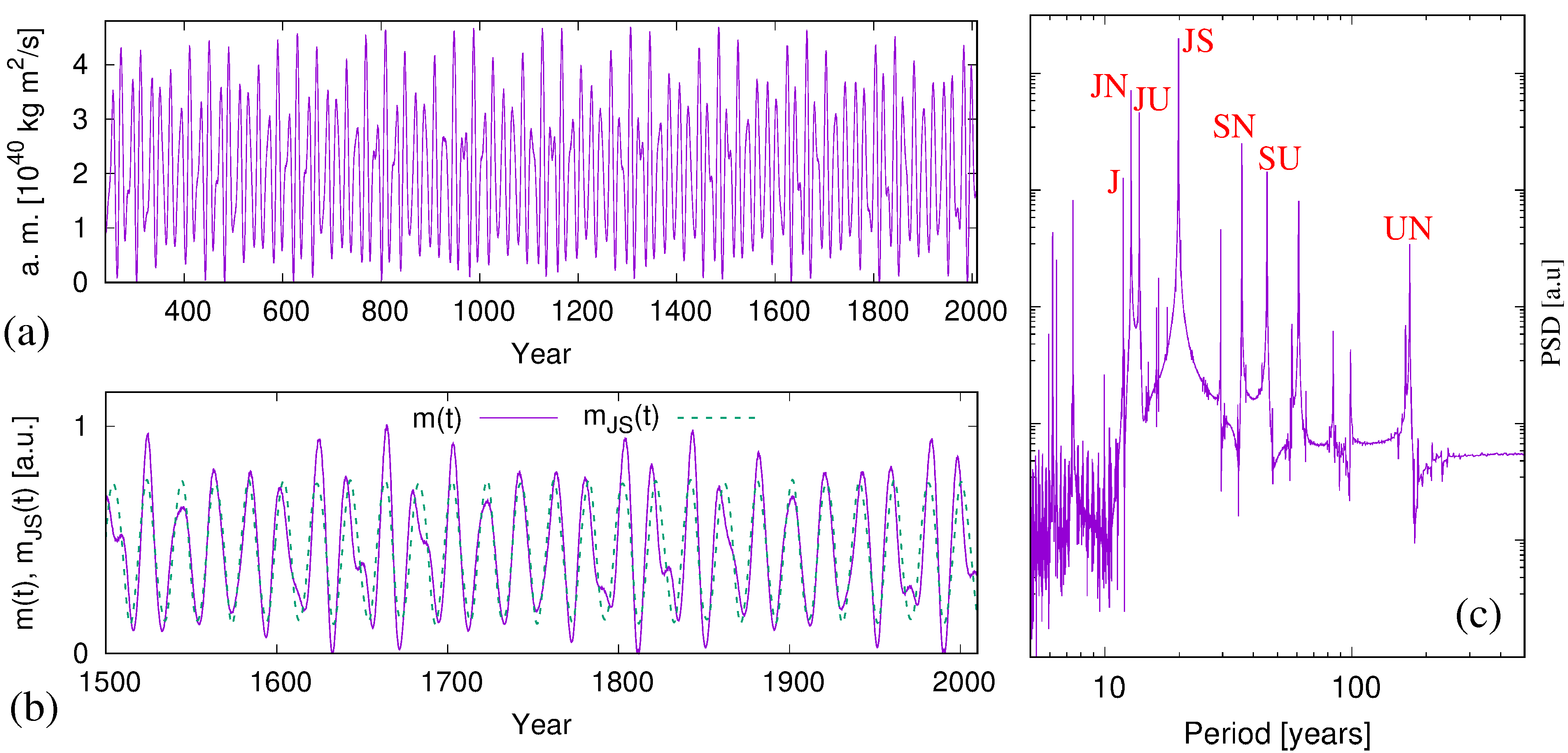
Figure 2.: (a) Time series of the orbital angular momentum (a.m.) of the Sun around the barycenter of the solar system during the interval A.D. 240-2010, based on the DE431 ephemerides (Folkner et al., 2014). (b) Zoom of (a) for the interval A.D. 1500-2010, normalized to 1, giving the modulation function $m(t)$ (violet full line). The corresponding function $m_{\rm JS}$ (green dashed) is a theoretical line that would result from the exclusive action of Jupiter and Saturn. (c) PSD of the angular momentum for the long interval 13199 B.C.-A.D. 17000, with some individual peaks attributed to planetary synodes (cf. Scafetta et al. (2016)): JN: Jupiter-Neptune (12.78 years), JU: Jupiter-Uranus (13.95 years), JS: Jupiter-Saturn (19.86 years), SN: Saturn-Neptune (35.87 years), SU: Saturn-Uranus (45.36 years), UN: Uranus-Neptune (171.39 years). J indicates the 11.86 years period of Jupiter. Fig:angular

For the computation of the Sun’s orbital angular momentum we utilized the DE431 ephemerides (Folkner et al., 2014) in the time interval between 13199 B.C.-A.D. 17000, of which a $\approx$1800-years segment is visualized in Figure Fig:angular(a). This function is dominated by the 19.86-years synodes of Jupiter and Saturn, to which further contributions, mainly from Uranus and Neptun, are added (see the PSD in Figure Fig:angular(c)). Further below, we will use the normalized version $m(t)$ of this angular momentum curve for parametrizing the time-variation of $\kappa(t)$. For the sake of comparison, we will also assess the results for a modified variant $m_{\rm JS}(t)$ which relies exclusively on the 19.86-years periodic motion of Jupiter and Saturn.

3 Results

In this section, we present and discuss numerical results for a sequence of parameters similar to those utilized in Stefani et al. (2020a). The main difference is the much longer simulation time of 30 kyears, which is actually the interval for which the orbital angular momentum of the Sun was available to us (Folkner et al., 2014). Such longer simulations will allow for a more systematic study of the typical breakdowns of the 193-years modulated wave, and some preliminary comparisons with the sequence of Bond events. Another difference to Stefani et al. (2020a) is that here we focus chiefly on the noise-free case in order to evidence the intermittent route to deterministic chaos. A few results with noise included will nevertheless be presented at the end of the section and in the Appendix.

3.1 All planets, no noise

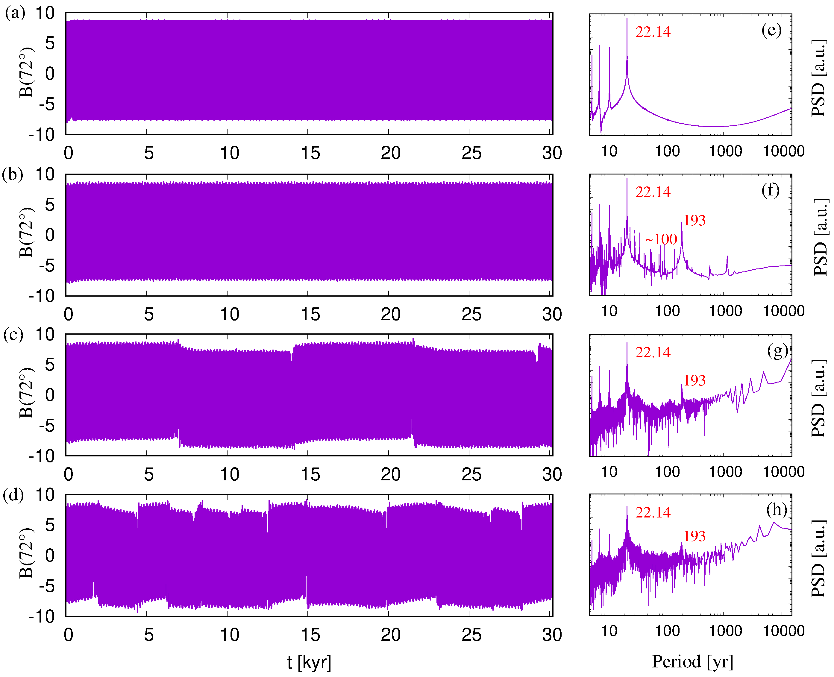
Figure 3.: (a-d) Time evolution of $B(72^{\circ},t)$, and its Lomb-Scargle PSD (e-h), with the common parameters $\omega_{0}=10000$, $\alpha^{c}_{0}=15$, $\alpha^{p}_{0}=50$ $q^{p}_{\alpha}=0.2$, $q^{c}_{\alpha}=0.8$, $D=0$. The time variation of the parameter $\kappa(t)$ increases from top to bottom. (a,e): $\kappa(t)=0.6$, a tidally synchronized dynamo producing a dipole with 22.14-year period. Note already the slight positive-negative asymmetry of $B(72^{\circ},t)$. (b,f): $\kappa(t)=0.6+0.3m(t)$, as (a,e), but with a modulation of $\kappa$ with an angular momentum function $m(t)$ according to Figure Fig:angular(b). As seen in the spectrum (f), this dipole solution contains a beat period of 193 years, which also appears in (b) as a minor wiggle of $B(72^{\circ},t)$. Note the appearance of Gleissberg-type cycles around 100 years in (f). (c,g): $\kappa(t)=0.6+0.32m(t)$, as (b,f), but with a slightly increased variation of $\kappa$. Note the appearance in (c) of four sudden events, where the positive-negative asymmetry of $B(72^{\circ},t)$ changes sign. The spectrum (g) has become noisy. (d,h): $\kappa(t)=0.6+0.4m(t)$, as (c,g), but with increased variation of $\kappa$, producing significantly more breakdowns. Fig:fiveexamples

Figure Fig:fiveexamples summarizes four different dynamo simulations carried out over an interval of 30.2 kyears. The time series of $B(\Theta=72^{\circ},t)$ are illustrated in the left panels (a-d), whose “patchy” appearances simply result from the large number ($\sim 1350$) of Hale cycles involved (more details will be shown further below). The right panels (e-h) show the associated power spectral densities (PSD) resulting from Lomb-Scargle analyses of the respective curves in (a-d).

The fixed parameters $\omega_{0}=10000$, $\alpha^{c}_{0}=15$, $\alpha^{p}_{0}=50$ $q^{p}_{\alpha}=0.2$, $q^{c}_{\alpha}=0.8$, $D=0$ are chosen similar to those of previous studies (Stefani, Giesecke and Weier, 2019; Stefani et al., 2020a), but note the complete absence of noise in the present runs. Moreover, here we set out with a sufficiently large value of $\alpha^{p}_{0}$ so that the dynamo is already synchronized to 22.14 years; the parametric resonance phenomenon behind the frequency synchronization, when going over from $\alpha^{p}_{0}=0$ to some finite value, had been discussed in detail in Stefani, Giesecke and Weier (2019); Stefani et al. (2020a) and will not be re-iterated here. Hence, the only parameter to be varied from top to bottom of Figure Fig:fiveexamples is the loss parameter $\kappa$.

We start in Figure Fig:fiveexamples(a,e) with a time-independent value $\kappa(t)=0.6$, which yields a very clean Hale cycle with a period 22.14 years. Already in panel (a) we observe a slight asymmetry between positive values (reaching $\approx 9$) and negative values (reaching $\approx-8$) that can be attributed to the presence of a mixed mode, in which a weak quadrupolar field component part is added to the dominant dipolar one. This effect is related to the Gnevyshev-Ohl rule (Gnevyshev and Ohl, 1948). Apart from the two minor peaks at the doubled and tripled Hale frequency (which naturally result from the nonlinear terms in the PDE system) the spectrum in (e) is quite smooth and featureless.

This is changing in Figure Fig:fiveexamples(b,f) when the loss parameter is equipped with a time-variation according to $\kappa(t)=0.6+0.3m(t)$, where $m(t)$ is the normalized orbital angular momentum function from Figure Fig:angular(b). The most prominent feature that appears in the PSD (f) is the strong peak at 193 years. In panel (b) this peak manifests itself in form of minor wiggles of the maxima and minima, which indeed correspond to a modulation of the positive-negative asymmetry. We note in passing the occurrence of some peaks at Gleissberg-type periods (around 96 years and 64 years), and two side bands at around 20 and 25 years which are reminiscent of the Wilson gap (Hathaway, 2010). These two features were discussed in more detail in Stefani et al. (2020a), and will not play a particular role in the following.

When increasing the variation of the loss parameter just a little further to $\kappa(t)=0.6+0.32m(t)$, we observe in panel (c) four sudden jumps of the positive-negative asymmetry. While the main peaks at 22.14 years and 193 years survive, the rest of the spectrum (g) becomes noisy, an effect of spectral leakage due to the segmentation of the entire time domain into 5 parts. While in this case one might still speculate about a regular occurrence of these breakdowns (with a waiting time of appr. 7 kyears), any alleged regularity is clearly lost in our last example (d,h), corresponding to $\kappa(t)=0.6+0.4m(t)$. Here we observe approximately 11 breakdowns without any clear periodicity. This insinuates an intermittent route to chaos, although we leave the detailed analysis of this transition, for our non-trivial case of double synchronized system, to future work.

For three of the examples from Figure Fig:fiveexamples, some details are discussed in the following. Figure Fig:kappavar0 shows the central interval between 14 and 16 kyears from Figure Fig:fiveexamples(a), both for $B(72^{\circ},t)$ (a) and for the entire field $B(\theta,t)$ as shown here as a contour-plot (b). In panel (a) we observe again the positive-negative asymmetry (the value varies between -8 and +9), which translates into a North-South asymmetry as visible in (b) by the color asymmetry between Northern and Southern regions. Evidently this asymmetry is also connected with a Gnevyshev-Ohl rule.

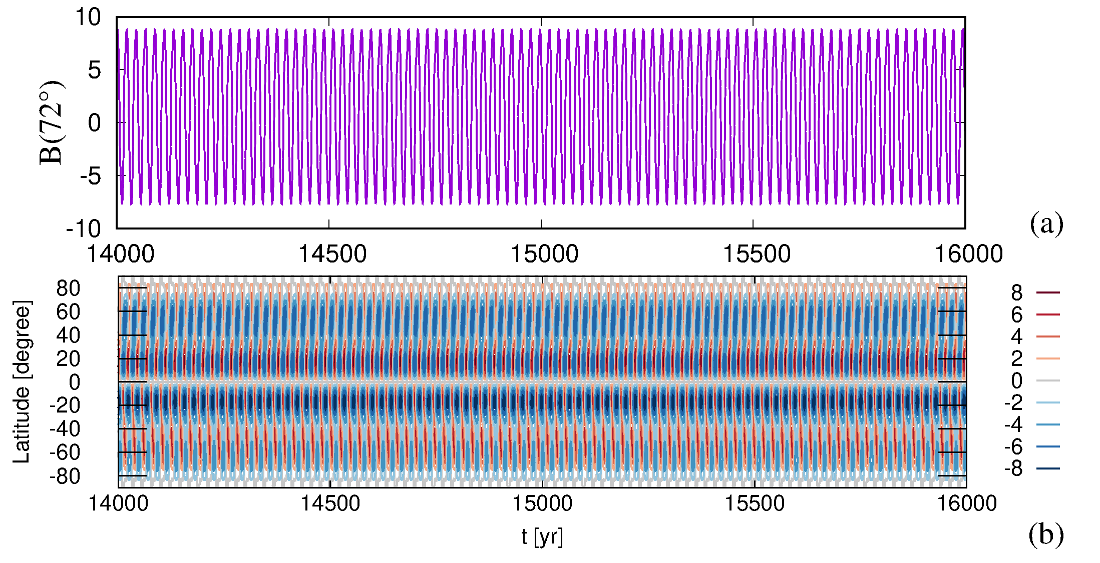
Figure 4.: (a) Details of Figure Fig:fiveexamples(a) for the central interval between 14000 and 16000 years, with parameters $\omega_{0}=10000$, $\alpha^{c}_{0}=15$, $\alpha^{p}_{0}=50$ $q^{p}_{\alpha}=0.2$, $q^{c}_{\alpha}=0.8$, $D=0$, $\kappa=0.6$. (b) Contour-plot of $B(\theta,t)$ for the same parameters. Note that in (b) the ordinate axis represents not the colatitude $\theta$ but the normal solar latitude $90^{\circ}-\theta$.Fig:kappavar0

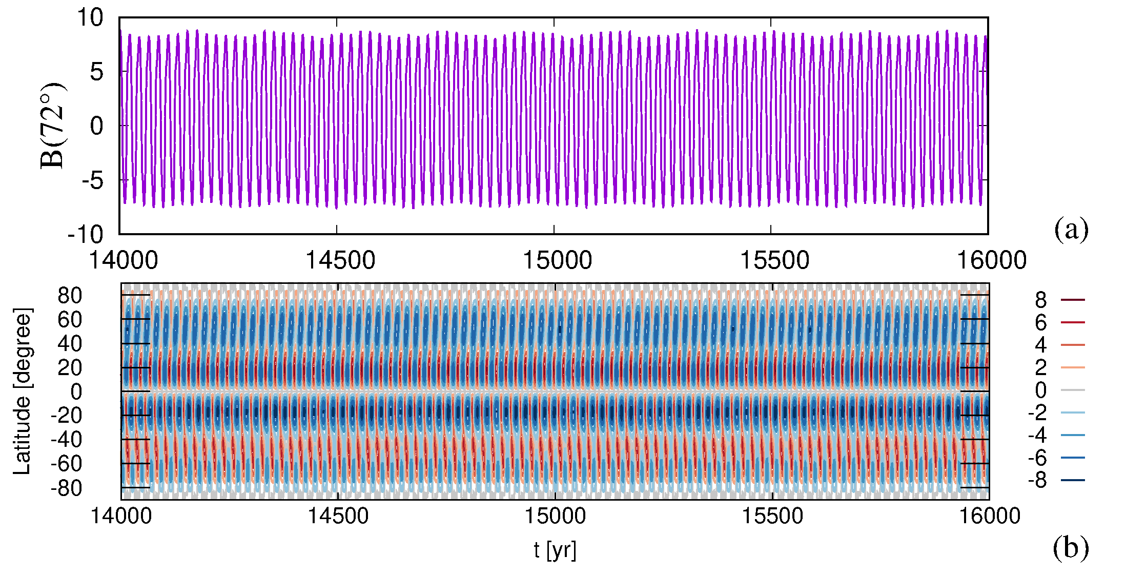
Figure 5.: Same as Figure Fig:kappavar0, but for Figure Fig:fiveexamples(b) with $\kappa=0.6+0.3m(t)$.Fig:kappavar03

A clear 193-years modulation of the positive-negative asymmetry, and the Gnevyshev-Ohl effect related to it, appears in Figure Fig:kappavar03 which illustrates some details of Figure Fig:fiveexamples(b). For the central interval of Figure Fig:fiveexamples(d), with $\kappa=0.6+0.4m(t)$, Figure Fig:kappavar04 shows one typical breakdown of the modulated wave. The resulting disordered state, lasting appr. 500 years, resembles indeed a cluster of grand minima where the dynamo is not switched off (Beer, Tobias and Weiss, 1998), but just in another state. Quite interesting here is the appearance of hemispherical fields (around 14900) and quadrupole fields (around 15000), which are reminiscent of sunspot observations within or shortly after the Maunder minimum (Sokoloff and Nesme-Ribes, 1994; Arlt, 2009). The corresponding trajectory in the dipole-quadrupole space, as shown in Figure Fig:dipole-quadrupole, resembles strongly the corresponding behaviour in Figure 5a of Knobloch, Tobias and Weiss (1998) and Figure 4 of Weiss and Tobias (2016). Meanwhile, a similar supermodulation effect has a also been found in a 3D simulation of dynamo action in rotating anelastic convection (Raynaud and Tobias, 2016).

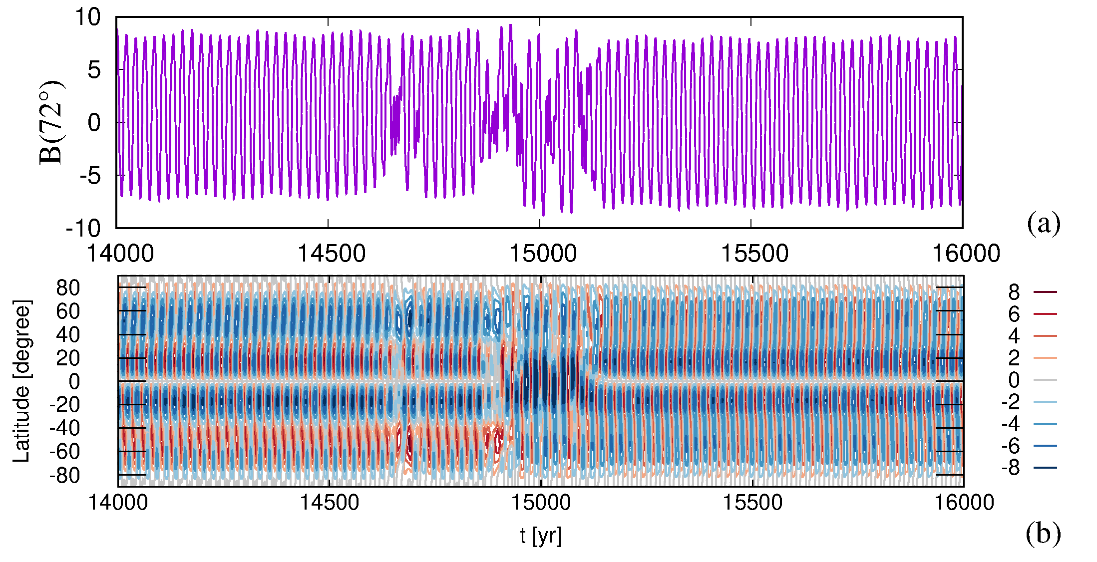
Figure 6.: Same as Figure Fig:kappavar0, but for Figure Fig:fiveexamples(d) with $\kappa=0.6+0.4m(t)$.Fig:kappavar04

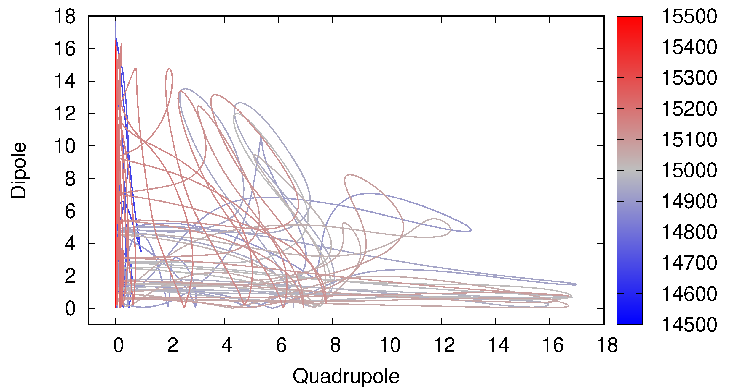
Figure 7.: Trajectory of the solution from Figure Fig:kappavar04 for the shortened interval between 14500-15500 years. The abscissa shows the quadrupolar component defined here as $|B(72^{\circ})+B(108^{\circ})|$, the corresponding dipolar component $|B(72^{\circ})-B(108^{\circ})|$ is shown on the ordinate axis.Fig:dipole-quadrupole

3.2 Only Jupiter and Saturn, no noise

We now consider a modification of the angular momentum that enters the time-variation of the loss parameter $\kappa(t)$. While in the previous subsection the full (normalized) angular momentum curve $m(t)$ was used (violet full line in Figure Fig:angular(b)), we consider now the idealized curve $m_{\rm JS}(t)$ as it would result from exclusively taking into account the orbital motion of Jupiter and Saturn (green dashed curve in Figure Fig:angular(b)).

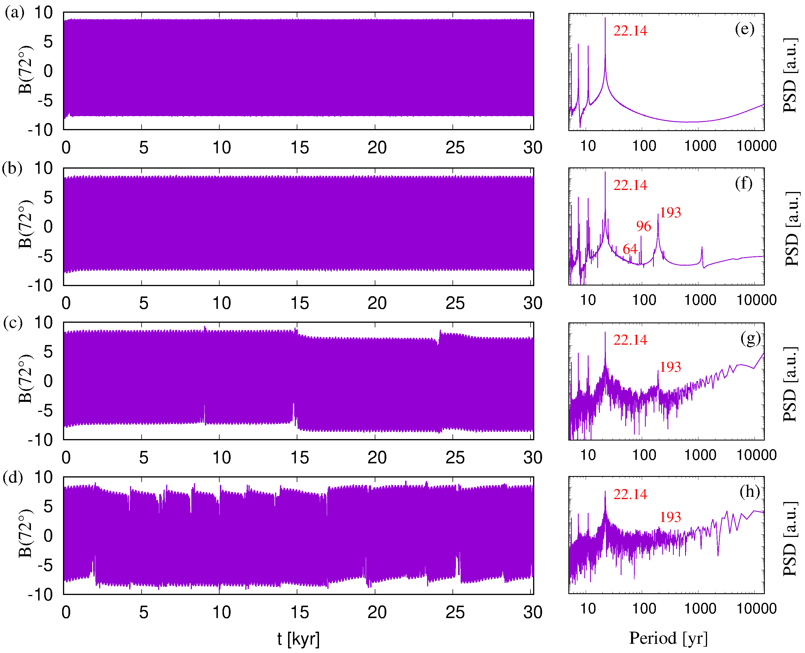
Figure 8.: Same as Figure Fig:fiveexamples but with the simpler angular momentum variation $m_{\rm JS}(t)$ (green dashed line in Figure Fig:angular(b)) which is restricted to the 19.86-years periodic part resulting from the orbital motion of Jupiter and Saturn only. Fig:simple

Figure Fig:simple shows the corresponding numerical results for otherwise the same parameters as used previously in Figure Fig:fiveexamples. Superficially, the results are very similar, with the most significant differences showing up for the range of Gleissberg-type periods. With the simplified $m_{\rm JS}(t)$curve, we observe now clean peaks at one half (96.5 years) and one third (64.3 years) of the 193-years beat period, whereas in Figure Fig:fiveexamples those peaks were more complicated. In Figure Fig:period_vergleich we summarize our present understanding regarding the origin of the different peaks. The PSD for $m(t)$ (violet) is a reproduction from Figure Fig:angular(c). It is dominated by the Jupiter-Saturn-peak at 19.86 years, and some other peaks, including the Jupiter-Neptune synode (12.78 years) and the Jupiter-Uranus synode (13.81 years). Both for the field resulting from $m(t)$ and from $m_{\rm JS}(t)$, the two dominant peaks are the Hale period (22.14 years) and the Suess-de Vries period (193 years). While the (blue) field curve for $m_{\rm JS}(t)$ contains basically only one half (96.5 years) and one third (64.3 years) of this Suess-de Vries period, the (green) curve for the full $m(t)$ contains additional peaks in the Gleissberg-region, comprising in particular the peaks at 55.8 years and 82.7 years which are beat periods between the 11.07-years Schwabe cycle and the Jupiter-Uranus synode (13.81 years) and Jupiter-Neptune synode (12.78 years), respectively. Moreover, a few additional peaks, indicated by question marks, seem to be related, e.g., to the Saturn-Neptun (35.87 years) and the Saturn-Uranus (44.36 years) synodes.

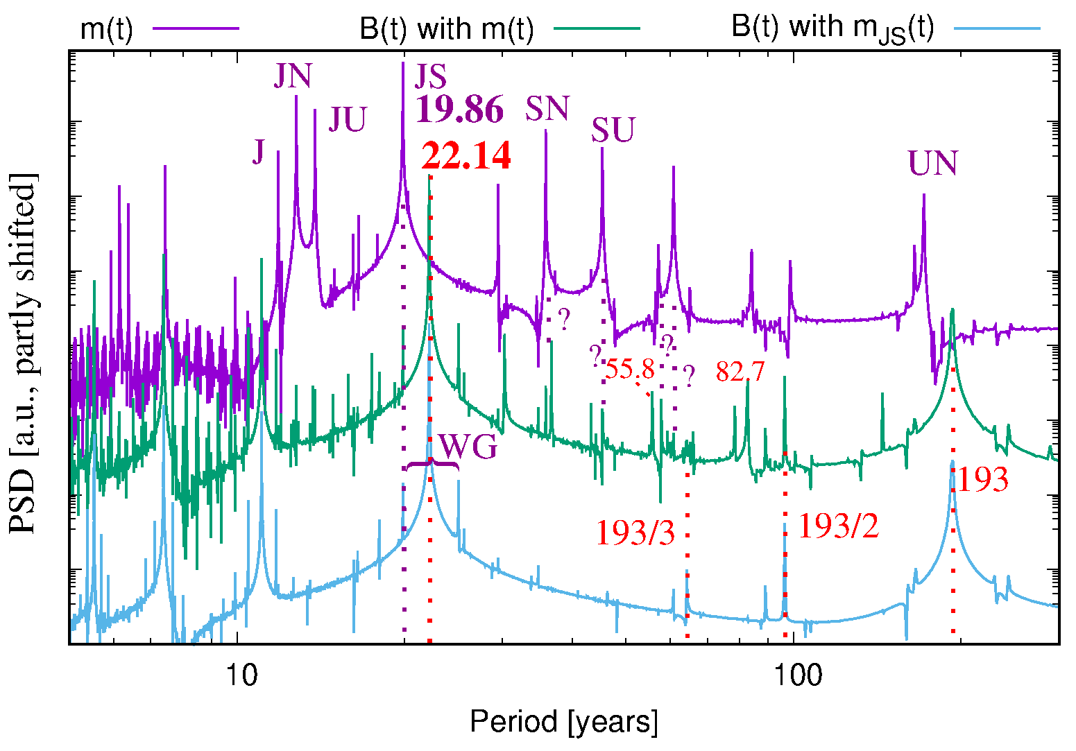
Figure 9.: Comparison of the Lomb-Scargle PSDs for the angular momentum function m(t) (violet), for $B(72^{\circ},t)$ (green) resulting from $\kappa(t)=0.6+0.3m(t)$ with the full $m(t)$, and for $B(72^{\circ},t)$ (blue) resulting from $\kappa(t)=0.6+0.2m_{\rm JS}(t)$ with the reduced $m_{\rm JS}(t)$. The individual peaks of the PSD for $m(t)$ are the same as in Figure Fig:angular(c). The Suess-de Vries period of 193 years, as well Gleissberg-type periods 193/2 and 193/3 years emerge already when using only $m_{\rm JS}(t)$. Some more peaks, which appear when the full $m(t)$ is utilized, can be attributed to corresponding peaks in $m(t)$ (see the question marks). However, there are two additional peaks at 55.8 years and 82.7 years which represent beat periods between the 11.07-years Schwabe cycle and the Jupiter-Uranus synode (13.81 years) and the Jupiter-Neptune synode (12.78 years), respectively. WG denotes the Wilson gap between 19.86 and 25 years.Fig:period˙vergleich

3.3 All planets, noise included

In Figure Fig:noise we assess the role of noise. The parameters are identical to those in Figure Fig:fiveexamples, except that we use now a finite noise level $D=0.05$. Not surprisingly, even without any $\kappa$ variation (a), the spectrum (e) is already noisy, while the positive-negative asymmetry in (a) is very similar to Figure Fig:fiveexamples(a). Apart from that, the overall structure turns out to be quite comparable to Figure Fig:fiveexamples.

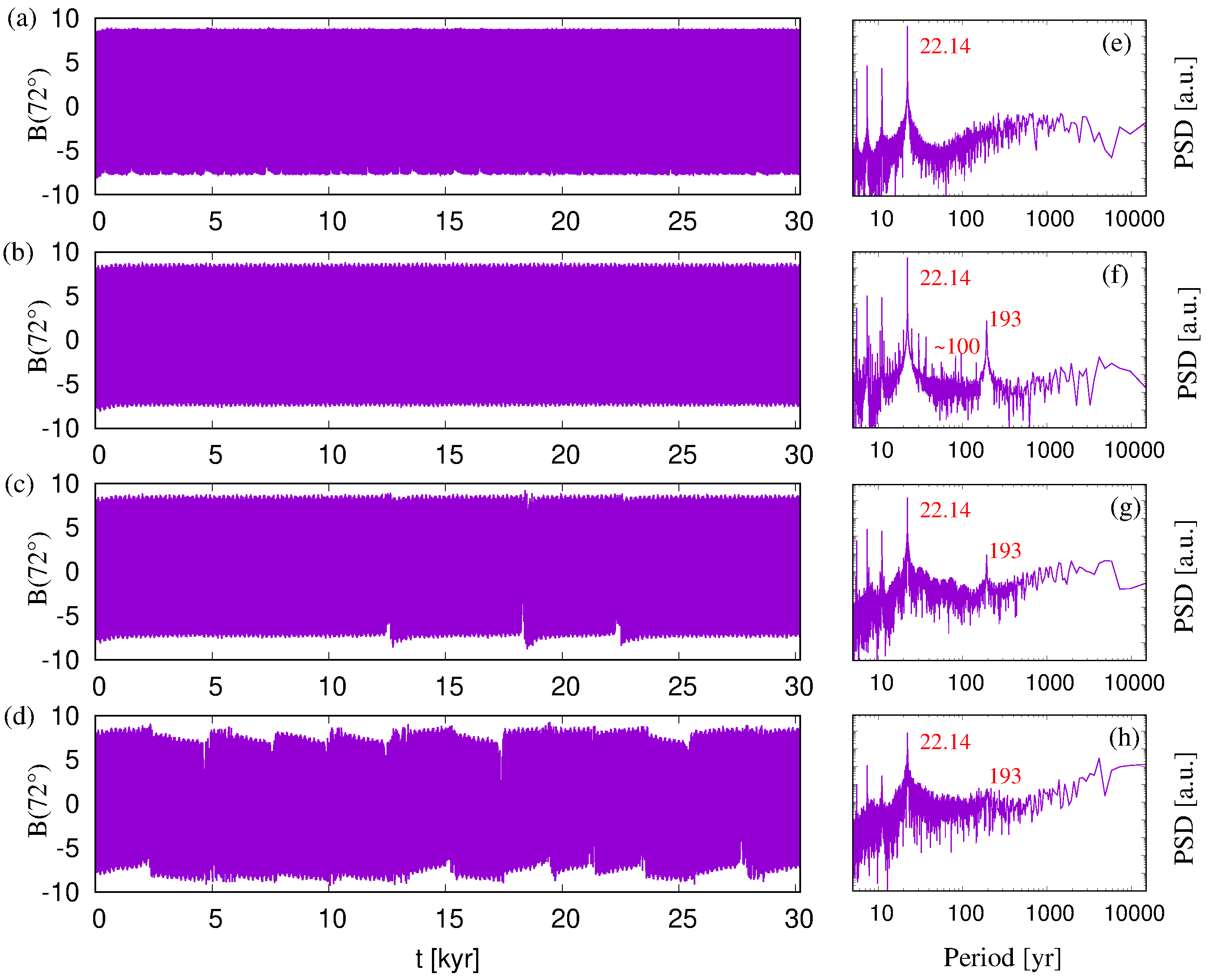
Figure 10.: Same as Figure Fig:fiveexamples but with noise intensity $D=0.05$. Even without any $\kappa$ variation, the spectrum (e) is already noisy, while the positive-negative asymmetry in (a) is very similar to that in Fig:fiveexamples(a). Apart from that, the overall structure, including the critical value for the transition to chaos, is very similar as for $D=0$.Fig:noise

If we go beyond the examples of Figure Fig:noise by choosing a still stronger variation $\kappa=0.6+0.5m(t)$, we end up with Figure Fig:kappavar05 which shows now a longer segment between 4-16 kyears. While for such long simulations many details are lost in the contour-plot (b), it highlights the fact that the breakdowns occur at instants where the North-South asymmetry (evidenced in particular by the reddish parts) has acquired a certain critical threshold. This entire behaviour is reminiscent of the supermodulation described by Weiss and Tobias (2016); Raynaud and Tobias (2016).

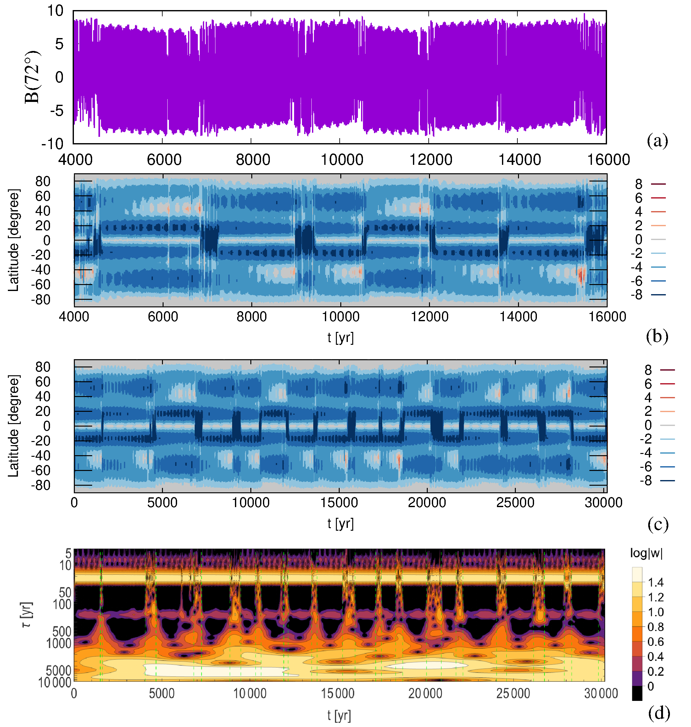
Figure 11.: (a) Behaviour of $B(72^{\circ},t)$ for $\omega_{0}=10000$, $\alpha^{c}_{0}=15$, $q^{p}_{\alpha}=0.2$, $q^{c}_{\alpha}=0.8$, $\alpha^{p}_{0}=50$, $D=0.05$ and $\kappa=0.6+0.5m(t)$, in the time interval 4000-16000 years. (b) Contour plot of $B(\theta,t)$ for the same parameters. (c) Contour-plot for the full time interval 0-30200 years. (d) Wavelet diagram for the full time interval. The green dashed lines in (d) indicate the intervals of breakdowns.Fig:kappavar05

With Figure Fig:kappavar05(c) we add a contour-plot for the full 30-kyears simulation period, just to illustrate the sequence of 17 breakdowns which were used for the numerical curve in Figure fig:bond_and_sim (where the time direction is inverted, though). As seen in Figure fig:bond_and_sim(b), those 17 events seem to obey the same random walk law as the 54 Bond events, although our 30-kyears simulation time is still too short for a convincing statistics. An interesting feature becomes visible in the wavelet spectrogram of Figure Fig:kappavar05(c) for $B(72^{\circ},t)$, which shows the distribution of oscillations with period $\tau$ in the vicinity of time $t$. During the breakdowns, characterized by a reduced energy in the 22.14-years period, we observe a significant increase of the energy in a wide range of $\tau$ from 30 to 1000-years. In fact the spectrum seems to become continuous here which reflects a transition to chaos due to nonlinearity. The quantitative difference between “regular” and “chaotic” regimes is highlighted in Figure Fig:chaos_regular which shows the wavelet spectral density integrated over the corresponding intervals, separated by the green dashed lines in Figure Fig:kappavar05(d). With the energy in the $\tau$-range from 30 to 1000-years being generally increased in the “chaotic” segments by 1-2 orders of magnitude, the particular peak around 200-years is still markedly pronounced. A corresponding behaviour had been reported in Figure 6 of McCracken, Beer and Steinhilber (2013).

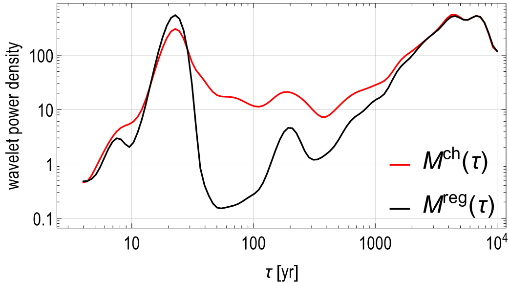
Figure 12.: Comparison of the wavelet power density for the “chaotic” intervals (separated by the green dashed lines in Figure Fig:kappavar05(d)) with that for the remaining “regular” intervalsFig:chaos˙regular

In the Appendix, we will carry out a similar analysis as in Figure Fig:kappavar05 but for the case of fixed $\kappa=0.6$ without any time variation but stronger noise with $D=0.1$. We will then also find breakdown regions but no particular role of the Suess-de Vries cycle.

4 Summary and open problems

In this paper we have pursued the ambitious program of finding a more or less complete and self-consistent description of the most significant periodicities (and time-scales) of the solar dynamo. First, we recapitulated the basic idea that the 22.14-years Hale cycle is synchronized by the 11.07-years tidal ($m=2$) forcing period of the tidally dominant VEJ-system, the importance of which had been pointed out earlier by Hung (2007); Scafetta (2012); Wilson (2013); Okhlopkov (2014, 2016). In various numerical models (Stefani et al., 2016, 2018; Stefani, Giesecke and Weier, 2019) this (weak) tidal forcing was supposed to trigger a resonant excitation of 11.07-years oscillations of that part of the $\alpha$-effect which is related to a typical $m=1$ instability within or close to the tachocline, such as the Tayler instability or a magneto-Rossby wave. Strong empirical evidence for a phase coherent 11.07-year Schwabe cycle comes both from algae data in the early Holocene (Vos et al., 2004), and from ¹⁴C and ¹⁰B data for the last 600 years (Stefani et al., 2020b). We note in passing that the numerical models produce, via the resonant dependence of the $\alpha$-effect on the magnetic field strength, also secondary peaks of solar activity, which might be linked to mid-term oscillations (Obridko and Shelting, 2007; Valdés-Galicia and Velasco, 2008; McIntosh et al., 2015; Bazilevskaya et al., 2016; Karak, Mandal and Banarjee, 2018; Frick et al., 2020).

Second, motivated by ideas of Cole (1973); Wilson (2013); Solheim (2013), we argued that the Suess-de Vries cycle emerges as a 193-years beat period between the primary, tidally synchronized 22.14-years Hale cycle and the single strongest component of solar motion around the barycenter of the planetary system, which is governed by the 19.86-years synodic cycle of Jupiter and Saturn. Without a detailed model for spin-orbit coupling at hand, we hypothesized that this coupling would lead to a periodic variation of the field loss parameter $\kappa$ in the tachocline region. Numerically, the combination of such a $\kappa$-variation with the synchronized component of the $\alpha$-effect led to a modulation of the dynamo wave with a beat period of 193 years, which manifests itself in a modulation of the North-South asymmetry and, closely related to that, in a change of the dipole-quadrupole relation (Knobloch, Tobias and Weiss, 1998; Moss and Sokoloff, 2017) and the Gnevyshev-Ohl rule. We would like to point out that the emergence of this beat period depends critically on the phase stability of the two underlying 11.07-years and 19.86-years processes, or, to put it otherwise: the existence of the long-term Suess-de Vries cycle gives a “backward argument” for the synchronized character of the short-term Hale cycle. As discussed in detail in Stefani et al. (2020a) (but only shortly touched upon in this paper), a stronger variation of $\kappa$ leads to the occurrence of a Wilson gap (Wilson, 1987) with two side peaks at 19.86 years and 25 years. Some aspects of this behaviour were illustrated in Figure Fig:period_vergleich.

The main focus of this paper was, however, on the intermittent occurrence of grand minima, and clusters thereof. We have observed irregular breakdowns of the 193-years modulated dynamo wave, preferably at instants where the North-South asymmetry reaches a certain critical level. This threshold effect fits well to a corresponding observation of Tlatov (2013) for the Maunder and Dalton minima. Since those irregular breakdowns are already observed in the absence of any noise, they seem to be connected with an intermittent transition to (deterministic) chaos, similar as in the supermodulation concept developed by Weiss and Tobias (2016). For an appropriately chosen time-variation of $\kappa$ (and some weak noise), we obtained a waiting time distribution with a similar mean value and standard deviation as inferred from the 54 Bond cycles observed over the last 80 kyears. Such an intermittent transition to chaos would hamper any long-term predictability of solar activity (and the climatic changes connected with it), even if the planetary clocking of the shorter-term Hale and Suess-de Vries cycles could be confirmed.

Based on a conventional $\alpha-\Omega$-dynamo, our model thus required only the two synchronization periods 11.07 years and 19.86 years, related to tidal forcing and the strongest component of solar orbital motion, respectively, to produce essentially all relevant periods, and “periods”, of the solar dynamo. While this appears promising, we conclude with a discussion of remaining problems and “missing links” in the theory.

First, we have to admit that, up to present, the basic synchronization mechanism for the helicity of an $m=1$ mode by some tide-like ($m=2$) forcing has been evidenced only for the paradigmatic case of a non-rotating, full cylinder (Stefani et al., 2016). Preliminary attempts for a hollow (more “tachoclinic”) cylinder were promising, although not entirely conclusive. Neither rotation nor stratification were implemented yet. A test of the same concept in the simplified framework of an $m=1$ buoyancy instability of toroidal flux rings, as developed by Ferriz Mas, Schmitt, and Schüssler (1994), could be very helpful and instructive in this respect. Interestingly, helicity synchronization with an $m=2$ forcing was numerically observed for the physically different, but topologically similar case of an $m=1$ large scale circulation of Rayleigh-Bénard convection in a cylinder (Galindo, 2020). A liquid metal experiment to confirm this effect is presently under way (Stepanov and Stefani, 2019; Jüstel et al., 2020).

As this suggests a generic and robust character of the helicity synchronization mechanism, there is good hope to apply the same principle also to the $m=1$ magneto-Rossby waves which were recently discussed by Dikpati et al. (2017); Marquez-Artavia, Jones, and Tobias, (2017); McIntosh et al. (2017); Zaqarashvili (2018). Unstable shallow-water modes had been shown earlier (Dikpati et al., 2009) to produce kinetic helicity, which is concentrated in the neighborhood of toroidal flux bands and migrates with them toward the equator as the solar cycle progresses. It should not be too complicated to implement a tide-like $m=2$ forcing into those shallow-water models in 2D (here: in $\theta$ and longitude $\phi$) with the aim to identify a similar helicity synchronization mechanism as found for the Tayler instability.

As a next step one could think about combining such a 2D model (in $\theta,\phi$) with another 2D model (in $\theta,r$) as it was utilized in various Babcock-Leighton type dynamo models (Guerrero and de Gouveia Dal Pino, 2007; Jouve et al., 2008). Presently we are working on an enhancement of the latter type of models in order to assess the direction of the butterfly diagram and to see whether a weak synchronized part of $\alpha$ (with an amplitude of less then 1 m/s, as limited by the argument of Öpik (1972)) is indeed sufficient for synchronizing the dynamo.

Turning to the spin-orbit coupling based on the 19.86-years orbital motion, and the resulting 193-years beat period, we first have to ask ourselves: does this beat period indeed correspond to the Suess-de Vries cycle? Since typical periods of this cycle between 190 until 210 years have been discussed in the literature, 193 years sounds not too bad in this respect. It also seems to be supported by a recent result of Ma and Vaquero (2020) who had found a 195-years period for the strong and clearly expressed Suess-de Vries cycle in the relatively “quiet” interval between 800 and 1340 A.D.

But even if the equivalence of the 193-years modulation with the Suess-de Vries could once be confirmed, we would still be left with the problem to explain the coupling of the (mainly) 19.86-years periodic orbit into some internal, dynamo relevant motion. To the best of our knowledge, there have been no serious attempts to tackle this problem in its full beauty, including a realistic orbital motion, the 7 degree inclination of the Sun’s rotation axis, and an alleged non-sphericity of the tachocline with a prolateness that might even vary with the magnetic field strength (Dikpati and Gilman, 2001). In this respect, we recall a relatively recent result on the similar problem of precession, for which a significant braking of the (solid body like) rotational profile was observed already for weak precessional forcing (Giesecke et al., 2018, 2019; Meunier and Albrecht, 2020). If such a braking effect would also occur in the solar spin-orbit coupling problem, it could indeed result in a change of the very sensitive adiabaticity (Abreu et al., 2012), and the associated $\kappa$ parameter as used here. Admittedly, this complex problem has to be left for future studies.

With the main focus laid on the synchronized helicity of $m=1$ instabilities, we should not overlook alternative synchronization mechanisms based on axisymmetric ($m=0$) instabilities, the relevance of which had been discussed by several authors (Dikpati et al., 2009; Rogers, 2011). The recent detection of a double-diffusive helical magnetorotational instability for flows with positive shear (Mamatsashvili et al., 2019) might be an interesting candidate in this respect, as it depends quite sensitively on the ratio of toroidal to poloidal field which, in turn, could be easily influenced by variations of $\kappa$.

In summary, given its skill in reproducing the various solar cycles, and “cycles”, with only mild (and indeed unessential) parameter fitting, our model looks like a reasonable choice for Occam’s razor to point toward. Yet, we cannot completely rule out that we were maliciously mislead by all those regularities and coincidences, that in reality the Schwabe cycle results from a peculiar self-synchronization mechanism (Hoyng, 1996), and that less “astrological” explanations will also be found for the long-term rhythms of our home star.

Acknowledgments

This project has received funding from the European Research Council (ERC) under the European Union’s Horizon 2020 research and innovation programme (grant agreement No 787544). The work was also supported in frame of the Helmholtz - RSF Joint Research Group “Magnetohydrodynamic instabilities: Crucial relevance for large scale liquid metal batteries and the sun-climate connection”, contract No HRSF-0044 and RSF-18-41-06201. We thank André Giesecke for a critical reading of an early version of the manuscript. Inspiring discussions with Jürg Beer, Antonio Ferriz Mas, Peter Frick, Rafael Rebolo, Günther Rüdiger, Dmitry Sokoloff, Willie Soon, and Ian Wilson on various aspects of the solar dynamo, and its synchronization, are gratefully acknowledged.

Disclosure of Potential Conflicts of Interest

The authors declare that they have no conflicts of interest.

Appendix

Figure Fig:noisedetails shows, for all parameters kept as in Figure Fig:kappavar05, except using constant $\kappa=0.6$ and slightly increased $D=0.1$, the occurrence of breakdowns under the exclusive influence of noise. Compared to Figure Fig:kappavar05 the behaviour seems to be different, with only one long-lasting change of the positive-negative and North-South asymmetry. Not surprisingly for this case without $\kappa$ variation, there is no particular peak at 193 years in the wavelet spectrogram (d). It seems that the transition to disorder/chaos is different in that case, and that the existence of a second frequency is decisive in this respect.

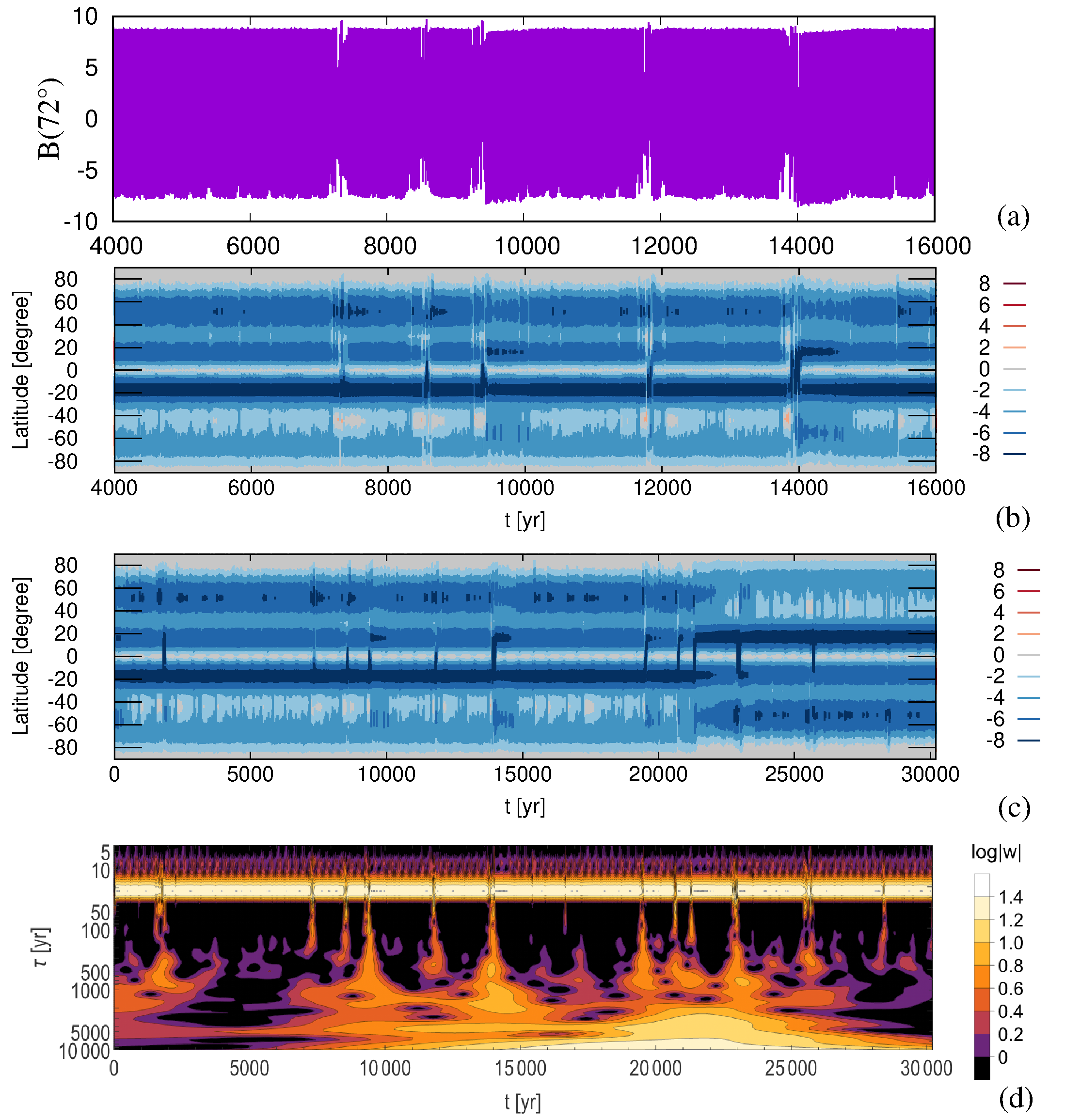
Figure 13.: (a) Behaviour of $B(72^{\circ},t)$ for $\omega_{0}=10000$, $\alpha^{c}_{0}=15$, $q^{p}_{\alpha}=0.2$, $q^{c}_{\alpha}=0.8$, $\alpha^{p}_{0}=50$, $D=0.1$ and $\kappa=0.6$, in the time interval 4000-16000 years. (b) Contour-plot of $B(\theta,t)$ for the same parameters. (c) Contour-plot for the full time interval 0-30200 years. (d) Wavelet diagram for the full time interval.Fig:noisedetails

References

- Abreu et al. (2012) Abreu, J.A., Beer, J., Ferriz-Mas, A., McCracken, K.G., Steinhilber, F.: 2012, Is there a planetary influence on solar activity? Astron. Astrophys. 548, A88. DOI.
- Arlt (2009) Arlt, R.: 2009, The butterfly diagram in the eighteenth century. Solar Phys. 255, 143. DOI.
- Bazilevskaya et al. (2016) Bazylevskaya, G.A. Kalinin, M.S., Krainev, M.B. Makhmutov, V.S. Svirzhevskaya, A.K. Svirzhevsky,, N.S. Stozhkov Y.I.: 2016, On the relationship between quasi-biennial variations of solar activity, the heliospheric magnetic field and cosmic rays. Cosmic Res. 54, 171. DOI.
- Beer, Tobias and Weiss (1998) Beer, J., Tobias, S., Weiss, N.: 1998, An active Sun throughout the Maunder minimum. Solar Phys. 181, 237. DOI.
- Bollinger (1952) Bollinger, C.J.: 1952, A 44.77 year Jupiter–Venus–Earth configuration Sun-tide period in solar-climatic cycles. Proc. Okla. Acad. Sci. 33, 307.
- Bond et al. (1997) Bond, G., Showers, W., Cheseby, M., Lotti, R., Almasi, P., deMenocal, P., Priore, P., Cullen, H., Haidas, I., Bonani, G.: 1997, A pervasive millennial-scale cycle in North Atlantic Holocene and glacial climates. Science. 278, 1257. DOI.
- Bond et al. (1999) Bond, G., Showers, W., Elliot, M., Evans, M. Lotti, R., Hajdas, I., Bonani, G., Johnson, S.: 1999, The North Atlantic’s 1-2 kyr climate rhythm: Relation to Heinrich events, Dansgard/Oeschger cycles and the Little Ice Age. Mechanisms of Global Climate Change at Millennial Time Scales. Geophysical Monograph Series. 112, 35. DOI.
- Bond et al. (2001) Bond, G., Kromer, B., Beer, J., Muscheler, R., Evans, M.N., Showers, W., Hoffmann, S., Lotti-Bond, R., Hajdas, I., Bonani, G.: 2001, Persistent solar influence on North Atlantic climate during the Holocene. Science. 294, 2130. DOI.
- Braun et al. (2005) Braun, H., Christl, M., Rahmstorf, S., Ganopolski, A. Mangini, A., Kubatzki, C., Roth, K., Kromer, B.: 2004, Possible solar origin of the 1,470-year glacial climate cycle demonstrated in a coupled model. Nature. 438, 208. DOI.
- Callebaut, de Jager, and Duhau (2012) Callebaut, D.K., de Jager, C., Duhau, S.: 2012, The influence of planetary attractions on the solar tachocline. J. Atmos. Sol.-Terr. Phys. 80, 73. DOI.
- Charbonneau (2010) Charbonneau, P.: 2010, Dynamo models of the solar cycle. Liv. Rev. Solar Phys. 7, 3. DOI.
- Charvatova (1997) Charvatova, I.: 1997, Solar-terrestrial and climatic phenomena in relation to solar inertial motion. Surv. Geophys. 18, 131. DOI.
- Cionco and Soon (2015) Cionco, R.G., Soon, W.: 2015, A phenomenological study of the timing of solar activity minima of the last millennium through a physical modeling of the Sun-Planets interaction. New Astron. 34, 164. DOI.
- Cionco and Pavlov (2018) Cionco, R.G., Pavlov, D.A.: 2018, Solar barycentric dynamics from a new solar-planetary ephemeris. Astron. Astrophys. 615, A153. DOI.
- Cole (1973) Cole, T.W.: 1973, Periodicities in solar activity. Solar Phys. 30, 103. DOI.
- Condon and Schmidt (1975) Condon, J.J., Schmidt, R.R.: 1975, Planetary tides and sunspot cycles. Solar Phys. 42, 529. DOI.
- De Jager and Versteegh (2005) De Jager, C., Versteegh, G.: 2005, Do planetary motions drive solar variability? Solar Phys. 229, 175. DOI.
- Dicke (1978) Dicke, R.H.: 1978, Is there a chronometer hidden deep in the Sun? Nature 276, 676.
- Dikpati and Gilman (2001) Dikpati, M., Gilman, P.A.: 2001, Prolateness of the solar tachocline inferred from latitudinal force balance in a magnetohydrodynamic shallow-water model. Astrophys. J. 552, 348. DOI.
- Dikpati et al. (2009) Dikpati, M., Gilman, P.A, Rempel, M.: 2003, Stability analysis of tachocline latitudinal differential rotation and coexisting toroidal band using a shallow-water model. Astrophys. J. 596, 680. DOI.
- Dikpati et al. (2009) Dikpati, M., Gilman, P.A, Cally, P.S., Miesch, M.S.: 2009, Axisymmetric MHD instabilities in solar/stellar tachoclines. Astrophys. J. 692, 1421. DOI.
- Dikpati et al. (2017) Dikpati, M., Cally, P.S., McIntosh, S.W., Heifetz, E.: 2017, The origin of the “Seasons” in Space Weather. Sci. Rep. 7, 14750. DOI.
- Dima and Lohmann (2009) Dima, M., Lohmann, G.: 2009, Conceptual model for millennial climate variability: a possible combined solar-thermohaline circulation origin for the 1,500-year cycle. Clim. Dyn. 32, 301. DOI.
- Fairbridge and Shirley (1987) Fairbridge, R.W., Shirley, J.H.: 1987, Prolonged minima and the 179-yr cycle of the solar inertial motions. Solar Phys. 110, 191. DOI.
- Ferriz Mas, Schmitt, and Schüssler (1994) Ferriz Mas, A., Schmitt, D., Schüssler, M.: 1994, A dynamo effect due to instability of magnetic flux tubes. Astron. Astrophys. 289, 949.
- Folkner et al. (2014) Folkner, W.M., Williams, J.G., Boggs, D.H., Park, R.S., Kuchynka, P.: 2014, The planetary and lunar ephemerides DE430 and DE431. IPN Progress Report 42-196, 1.
- Frick et al. (2020) Frick, P., Sokoloff, D., Stepanov, R., Pipin, V., Usoskin, I.: 2020, Spectral characteristic of mid-term quasi-periodicities in sunspot data. Mon. Not. R. Astron. Soc. 491, 5572. DOI.
- Galindo (2020) Galindo, V.: 2020, personal communication.
- Guerrero and de Gouveia Dal Pino (2007) Guerrero, G., de Gouveia Dal Pino, E.M.: 2007, How does the shape and thickness of the tachocline affect the distribution of the toroidal magnetic fields in the solar dynamo?. Astron. Astrophys. 464, 341. DOI.
- Giesecke et al. (2018) Giesecke, A., Vogt, T., Gundrum, T., Stefani, F.: 2018, Nonlinear large scale flow in a precessing cylinder and its ability to drive dynamo action. Phys. Rev. Lett. 120, 024502. DOI.
- Giesecke et al. (2019) Giesecke, A., Vogt, T., Gundrum, T.: Stefani, F.: 2019, Kinematic dynamo action of a precession-driven flow based on the results of water experiments and hydrodynamic simulations.. Geophys. Astrophys. Fluid Dyn. 113, 235. DOI.
- Gnevyshev and Ohl (1948) Gnevyshev, M.N., Ohl, A.I.: 1948, On the 22-year cycle of solar activity. Astron. J. 25, 18-20.
- Hathaway (2010) Hathaway, D.H.: 2015, The solar cycle. Liv. Rev. Sol. Phys. 12, 4. DOI.
- Howe (2009) Howe, R.: 2009, Solar interior rotation and its variation. Liv. Rev. Sol. Phys. 6, 1. DOI.
- Hoyng (1996) Hoyng, P.: 1996, Is the solar cycle timed by a clock? Solar Phys. 169, 253. DOI.
- Hung (2007) Hung, C.-C.: 2007, Apparent relations between solar activity and solar tides caused by the planets. NASA/TM-2007-214817.
- Jennings and Weiss (1991) Jennings, R.L., Weiss, N.O.: 1991, Symmetry breaking in stellar dynamos. Mon. Not. R. Astr. Soc. 252, 249. DOI.
- Jones (1983) Jones, C.A.: 1983, Model equations for the solar dynamo. In: Soward, A.M. (ed.) Stellar and Planetary Magnetism, Gordon and Breach, New York, 193.
- Jose (1965) Jose, P.D.: 1965, Sun’s motion and sunspots. Astron. J. 70, 193. DOI.
- Jouve et al. (2008) Jouve, L., Brun, A.S., Arlt, R., Brandenburg, A., Dikpati, M., Bonanno, A., Käpylä, P.J., Moss, D., Rempel, M., Gilman, P., Korpi, M.J., Kosovichev, A.G.: 2015, A solar mean field dynamo benchmark. Astron. Astrophys. 483, 949. DOI.
- Jüstel et al. (2020) Jüstel, P., Röhrborn, S., Frick, P., Galindo, V., Gundrum, T., Schindler, F., Stefani, F., Stepanov, R., Vogt, T.: 2020, Generating a tide-like flow in a cylindrical vessel by electromagnetic forcing. Phys. Fluids (submitted), arXiv:2006.03491.
- Karak, Mandal and Banarjee (2018) Karak, B.B., Mandal, S., Banarjee, D.: 2018, Double-peaks of the solar cycle: an explanation from a dynamo model. Astrophys. J. 866, 17. DOI.
- Knobloch, Tobias and Weiss (1998) Knobloch, E, Tobias, S.M., Weiss, N.O.: 1998, Modulation and symmetry changes in stellar dynamos. Mon. Not. R. Astron. Soc. 297, 1123. DOI.
- Kotov and Haneychuk (2020) Kotov, V.A., Haneychuk, V.I.: 2020, Oscillations of solar photosphere: 45 years of observations. Astro. Nachr. DOI.
- Kudryavtsev and Dergachev (2020) Kudryavtsev, I.V., Dergachev, V.A.: 2020, Reconstruction of heliospheric modulation potential based on radiocarbon data in the time interval 17000-5000 years B.C.. Geomagn. Aeron. 59, 1099. DOI.
- Kuzanyan and Sokoloff (1997) Kuzanyan, K.M., Sokoloff, D.: 1997, Half-width of a solar dynamo wave in Parker’s migratory dynamo. Solar Phys. 173, 1. DOI.
- Landscheidt (1999) Landscheidt, T.: 1999, Extrema in sunspot cycle linked to Sun’s motion. Solar Phys. 189, 413. DOI.
- Lüdecke, Weiss and Hempelmann (2015) Lüdecke, H.-J., Weiss, C.O., Hempelmann, A.: 2015, Paleoclimate forcing by the solar De Vries/Suess cycle. Clim. Past Discuss. 11, 279. DOI.
- Ma and Vaquero (2020) Ma, L., Vaquero, J.M., 2020 New evidence of the Suess/de Vries cycle existing in historical naked-eye observations of sunspots. Open Astron. 29, 28. DOI.
- Mamatsashvili et al. (2019) Mamatsashvili, G., Stefani, F., Hollerbach, R., Rüdiger, G.: 2019, Two types of axisymmetric helical magnetorotational instability in rotating flows with positive shear. Phys. Rev. Fluids, 4, 103905. DOI.
- Marquez-Artavia, Jones, and Tobias, (2017) Marquez-Artavia, X., Jones, C.A., Tobias, S.M.: 2017, Rotating magnetic shallow water waves and instabilities in a sphere. Geophys. Astrophys. Fluid Dyn. 111, 282. DOI.
- Mayewski et al. (1997) Mayewski, P.A., Meeker, L.D., Twickler, M.S., Whitlow, S., Yang, Q., Berry Lyons, W., Prentice, M.. 1997, Major features and forcing of high-latitude northern hemisphere atmospheric circulation using a 111,000-year-long glaciochemical series. J. Geophys. Res.: Oceans 102, 26345. DOI.
- McCracken, Beer and Steinhilber (2013) McCracken, K.G., Beer, J., Steinhilber, F., Abreu, J.: 2013, A phenomenological study of the cosmic ray variations over the Past 9400 years, and their implications regarding solar activity and the solar dynamo. Solar Phys. 286, 609. DOI.
- McCracken, Beer and Steinhilber (2014) McCracken, K.G., Beer, J., Steinhilber, F.: 2014, Evidence for planetary forcing of the cosmic ray intensity and solar activity throughout the past 9400 years. Solar Phys. 289, 3207. DOI.
- McIntosh et al. (2015) McIntosh, S.W. et al.: 2015, The solar magnetic activity band interaction and instabilities that shape quasi-periodic variability. Nature Comm. 6, 6491. DOI.
- McIntosh et al. (2017) McIntosh, S.W., Cramer, W.J., Pichardo Marcano, M, Leamon, R.J.: 2017, The detection of Rossby-like waves on the Sun. Nature Astron. 1, 0086. DOI.
- Meunier and Albrecht (2020) Meunier, P., Albrecht, T.: 2020, personal communication.
- Moss and Sokoloff (2017) Moss, D.L., Sokoloff, D.: 2017, Parity fluctuations in stellar dynamos. Astron. Rep. 61, 878. DOI.
- Muscheler et al. (2007) Muscheler, R. Joos, F. Beer, J. Müller, S.A. Vonmoos, M., Snowball, I.: 2007, Solar activity during the last 1000 yr inferred from radionuclide records. Quat. Sci. Rev., 26, 82. DOI.
- Obridko and Shelting (2007) Obridko, V.N., Shelting, B.D.: 2007, Occurrence of the 1.3-year periodicity in the large-scale solar magnetic field for 8 solar cycles. Adv. Space Res. 40, 1006. DOI.
- Okhlopkov (2014) Okhlopkov, V.P.: 2014, The 11-year cycle of solar activity and configurations of the planets. Mosc. Univ. Phys. B. 69, 257. DOI.
- Okhlopkov (2016) Okhlopkov, V.P.: 2016, The gravitational influence of Venus, the Earth, and Jupiter on the 11-year cycle of solar activity. Mosc. Univ. Phys. B. 71, 440. DOI.
- Öpik (1972) Öpik, E.: 1972, Solar-planetary tides and sunspots. I. Astron. J. 10, 298.
- Palus et al. (2000) Palus, M., Kurths, J., Schwarz, U., Novotna, D., Charvatova, I.: 2000, Is the solar activity cycle synchronized with the solar inertial motion? Int. J. Bifurc. Chaos 10, 2519. DOI.
- Parker (1955) Parker, E.N.: 1955, Hydromagnetic dynamo models. Astrophys. J. 122, 293. DOI.
- Pitts and Tayler (1985) Pitts, E., Tayler, R.J.: 1985, The adiabatic stability of stars containing magnetic-fields. 6. The influence of rotation. Mon. Not. Roy. Astron. Soc. 216, 139. DOI.
- Proctor (2007) Proctor, M.R.E.: 2007, Effects of fluctuations on dynamo models. Mon. Not. R. Astron. Soc. 382, L39. DOI.
- Raynaud and Tobias (2016) Raynaud, R., Tobias, S.M.: 2016, Convective dynamo action in a spherical shell: symmetries and modulation. J. Fluid Mech. 799, R6. DOI.
- Roald and Thomas (1997) Roald, C.B., Thomas, J.H.: 1997, Simple solar dynamo models with variable and effects. Mon. Not. R. Astron. Soc. 288, 551. DOI.
- Rogers (2011) Rogers, T.M.: 2011, Toroidal field reversals and the axisymmetric Tayler instability. Mon. Not. R. Astron. Soc. 288, 551. DOI.
- Rüdiger and Schultz (2020) Rüdiger, G., Schultz, M.: 2020, Large-scale dynamo action of magnetized Taylor-Couette flows. Mon. Not. R. Astron. Soc. 493, 1249. DOI.
- Scafetta (2012) Scafetta, N.: 2012, Does the Sun work as a nuclear fusion amplifier of planetary tidal forcing? A proposal for a physical mechanism based on the mass-luminosity relation. J. Atmos. Sol.-Terr. Phys. 81-82, 27. DOI.
- Scafetta et al. (2016) Scafetta, N., Milani, F., Bianchini, A., Ortolani, S.: 2016, On the astronomical origin of the Hallstatt oscillation found in radiocarbon and climate records throughout the Holocene. Earth Sci. Rev. 162, 24. DOI.
- Schmalz and Stix (1991) Schmalz, S., Stix, M.: 1991, An alpha-Omega dynamo with order and chaos. Astron. Astrophys. 245, 654.
- Schove (1983) Schove, D.J.: 1983, Sunspot Cycles, Hutchinson Ross Publishing Company, Stroudsburg.
- Seilmayer et al. (2012) Seilmayer, M., Stefani, F., Gundrum, T., Weier, T., Gerbeth, G., Gellert, M., Rüdiger, G.: 2012, Experimental evidence for a transient Tayler instability in a cylindrical liquid metal column. Phys. Rev. Lett. 108, 244501. DOI.
- Sharp (2013) Sharp, G.: 2013, Are Uranus and Neptune responsible for solar grand minima and solar cycle modulation? Int J. Astron. Astrophys. 3, 260. DOI.
- Sokoloff and Nesme-Ribes (1994) Sokoloff, D., Nesme-Ribes, E.: 1994, The Maunder minimum: a mixed-parity dynamo mode? Astron. Astrophys. 288, 293.
- Solheim (2013) Solheim, J.-E.: 2013, The sunspot cycle length - modulated by planets? Pattern Recogn. Phys. 1, 159.
- Soon et al. (2014) Soon, W., Velasco Herrera, V.M., Selvaraj, K., Traversi, R., Usoskin, I., Chen, C.A., Lou, J.Y. Kao, S.J., Carter, R.M., Pipin, V., Severi, M., Becagli, S.: 2014, A review of Holocene solar-linked climatic variation on centennial to millennial timescales: Physical processes, interpretative frameworks and a new multiple cross-wavelet transform algorithm. Earth Sci. Rev. 134, 1. DOI.
- Spruit (2002) Spruit, H.: 2002, Dynamo action by differential rotation in a stably stratified stellar interior. Astron. Astrophys. 381, 923. DOI.
- Stefani et al. (2016) Stefani, F., Giesecke, A., Weber, N., Weier, T.: 2016, Synchronized helicity oscillations: a link between planetary tides and the solar cycle? Solar Phys. 291, 2197. DOI.
- Stefani et al. (2017) Stefani, F., Galindo, V. Giesecke, A., Weber, N., Weier, T.: 2017, The Tayler instability at low magnetic Prandtl numbers: chiral symmetry breaking and synchronizable helicity oscillations. Magnetohydrodynamics 53, 169.
- Stefani et al. (2018) Stefani, F., Giesecke, A., Weber, N., Weier, T.: 2018, On the synchronizability of Tayler-Spruit and Babcock-Leighton type dynamos. Solar Phys. 293, 12. DOI.
- Stefani, Giesecke and Weier (2019) Stefani, F., Giesecke, A., Weier, T.: 2018, A model of a tidally synchronized solar dynamo. Solar Phys. 294, 60. DOI.
- Stefani et al. (2020a) Stefani, F., Giesecke, A., Seilmayer, M., Stepanov, R., Weier, T.: 2020, Schwabe, Gleissberg, Suess-de Vries: Towards a consistent model of planetary synchronization of solar cycles. Magnetohydrodynamics (in press), arxiv.org/abs/1910.10383.
- Stefani et al. (2020b) Stefani, F., Beer, J., Giesecke, A., Gloaguen, T., Seilmayer, R., Stepanov, R., Weier, T.: 2020, Phase coherence and phase jumps in the Schwabe cycle. Astron. Nachr. (submitted), arXiv:2004.10028.
- Steinhilber et al. (2012) Steinhilber, F. et al.: 2012, 9,400 years of cosmic radiation and solar activity from ice cores and tree rings. Proc. Natl. Acad. Sci. 109, 5967. DOI.
- Stepanov and Stefani (2019) Stepanov, R., Stefani, F.: 2019, Electromagnetic forcing of a flow with the azimuthal wave number m = 2 in cylindrical geometry. Magnetohydrodynamics 55, 207.
- Takahashi (1968) Takahashi, K.: 1968, On the relation between the solar activity cycle and the solar tidal force induced by the planets. Solar Phys. 3, 598. DOI.
- Tayler (1973) Tayler, R.J.: 1973, The adiabatic stability of stars containing magnetic fields-I: Toroidal fields. Mon. Not. Roy. Astron. Soc. 161, 365. DOI.
- Tlatov (2013) Tlatov, A.G.: 2013, Reversals of the Gnevyshev-Ohl rule. Astrophys. J. Lett. 772, L30. DOI.
- Usoskin et al. (2007) Usoskin, I.G., Solanki, S.K., Kovaltsov, G.A., 2007 Grand minima and maxima of solar activity: new observational constraints. Astron. Astrophys. 471, 301. DOI.
- Usoskin et al. (2016) Usoskin, I.G., Gallet, Y., Lopes, F., Kovaltsov, G.A., Hulot, G., 2016 Solar activity during the Holocene: the Hallstatt cycle and its consequence for grand minima and maxima. Astron. Astrophys. 587, A150. DOI.
- Valdés-Galicia and Velasco (2008) Valdés-Galicia, J.F., Velasco, V.M., 2008 Variations of mid-term periodicities in solar activity physical phenomena. Adv. Space. Res. 41, 297. DOI.
- Vos et al. (2004) Vos, H., Brüchmann, C., Lücke, A., Negendank, J.F.W., Schleser, G.H., Zolitschka, B.: 2004, Phase stability of the solar Schwabe cycle in Lake Holzmaar, Germany, and GISP2, Greenland, between 10,000 and 9,000 cal. BP In: Fischer, H., Kumke, T., Lohmann, G., Flöser, G., Miller, H., von Storch, H., Negendank, J. F. (Eds.), The Climate in Historical Times: Towards a Synthesis of Holocene Proxy Data and Climate Models, (GKSS School of Environmental Research), Springer, 293-318.
- Weber et al. (2013) Weber, N., Galindo, V., Stefani, F., Weier, T., Wondrak, T.: 2013, Numerical simulation of the Tayler instability in liquid metals. New J. Phys. 15, 043034. DOI.
- Weber et al. (2015) Weber, N., Galindo, V., Stefani, F., Weier, T.: 2015, The Tayler instability at low magnetic Prandtl numbers: between chiral symmetry breaking and helicity oscillations. New J. Phys. 17, 113013. DOI.
- Weiss and Tobias (2016) Weiss, N.O., Tobias, S.M: 2016, Supermodulation of the Sun’s magnetic activity: the effects of symmetry changes. Mon. Not. Roy. Astron. Soc. 456, 2654. DOI.
- Wilmot-Smith et al. (2006) Wilmot-Smith, A.L., Nandy, D., Hornig, G., Martens, P.C.H.: 2006, A time delay model for solar and stellar dynamos. Astrophys. J. 652, 696. DOI.
- Wilson (1987) Wilson, R.M.: 1987, On the distribution of sunspot cycle periods. J. Geophys. Res. 92, 10101.
- Wilson (2008) Wilson, I.R.G.: 2008, Does a spin-orbit coupling between the Sun and the Jovian planets govern the solar cycle?. Publ. Astron. Soc. Austr. 25, 85. DOI.
- Wilson (2013) Wilson, I.R.G.: 2013, The Venus-Earth-Jupiter spin-orbit coupling model. Pattern Recogn. Phys. 1, 147. DOI.
- Wolff and Patrone (2010) Wolff, C.L., Patrone, P.N.: 2010, A new way that planets can affect the sun. Solar Phys. 266, 227. DOI.
- Wood (1972) Wood, K.: 1972, Sunspots and planets. Nature 240(5376), 91. DOI.
- Zaqarashvili (1997) Zaqarashvili, T.: 1997, On a possible generation mechanism for the solar cycle.. Astrophys. J. 487, 930. DOI.
- Zaqarashvili (2018) Zaqarashvili, T.: 2018, Equatorial magnetohydrodynamic shallow water waves in the solar tachocline. Astrophys. J. 856, 32. DOI.