Performance bounds of non-adiabatic quantum harmonic Otto engine and refrigerator under a squeezed thermal reservoir

Abstract

We analyze the performance of a quantum Otto cycle, employing time-dependent harmonic oscillator as the working fluid undergoing sudden expansion and compression strokes during the adiabatic stages, coupled to a squeezed reservoir. First, we show that the maximum efficiency that our engine can achieve is 1/2 only, which is in contrast with the earlier studies claiming unit efficiency under the effect of squeezed reservoir. Then, we obtain analytic expressions for the upper bound on the efficiency as well as on the coefficient of performance of the Otto cycle. The obtained bounds are independent of the parameters of the system and depends on the reservoir parameters only. Additionally, with hot squeezed thermal bath, we obtain analytic expression for the efficiency at maximum work which satisfies the derived upper bound. Further, in the presence of squeezing in the cold reservoir, we specify an operational regime for the Otto refrigerator otherwise forbidden in the standard case.

I Introduction

The concept of Carnot efficiency ($\eta_{C}$) is one of the most important results in physics, which led to the formulation of the second law of thermodynamics Kondepudi and Prigogine (2014). It puts a theoretical upper bound on the efficiency of all macroscopic heat engines working between two thermal reservoirs at different temperatures. However, with the rise of quantum thermodynamics Vinjanampathy and Anders (2016); Mahler (2014); Deffner and Campbell (2019); Alicki and Kosloff (2018), many studies have showed that this sacred bound may be surpassed by quantum heat machines exploiting exotic quantum resources such as quantum coherence Scully (2001); Scully et al. (2003); Türkpençe and Müstecaplıoğlu (2016); Skrzypczyk et al. (2014), quantum correlations Bera et al. (2017); Park et al. (2013); Brunner et al. (2014); Perarnau-Llobet et al. (2015); Altintas et al. (2014), squeezed reservoirs Roßnagel et al. (2014); Huang et al. (2012); Kosloff and Rezek (2017); Agarwalla et al. (2017); Manzano et al. (2016); Xiao and Li (2018); Long and Liu (2015); Klaers et al. (2017); Correa et al. (2014); de Assis et al. (2020); Wang et al. (2019), among others. In such cases, the second law of thermodynamics has to be modified to account for the quantum effects, and the notion of generalized Carnot bound is introduced which is always satisfied Bera et al. (2017); Niedenzu et al. (2018); Abah and Lutz (2014); Roßnagel et al. (2014). In this context, different theoretical studies have been carried out to study the implications of work extraction when quantum heat machines are coupled to nonequilibrium stationary reservoirs Niedenzu et al. (2016); Alicki and Gelbwaser-Klimovsky (2015); Abah and Lutz (2014); Alicki (2014); Ghosh et al. (2018). In particular, it is instructive to look into the working of heat machines coupled to squeezed thermal reservoirs. The use of squeezed thermal reservoir allows us to extract work from a single reservoir Manzano et al. (2016), operate thermal devices beyond Carnot bound Klaers et al. (2017); Roßnagel et al. (2014); Manzano et al. (2016); Long and Liu (2015), define multiple operational regimes Manzano et al. (2016); Niedenzu et al. (2016) otherwise impossible for the standard case with two thermal reservoirs. Moreover, in Ref. Manzano (2018), the idea of treating squeezed thermal reservoir as a generalized equilibrium reservoir is explored. Recently, a nanomechanical engine consisting of a vibrating nanobeam coupled to squeezed thermal noise, operating beyond the standard Carnot efficiency, is realized experimentally Klaers et al. (2017).

Over the past few years, there have been increasing interest in investigating the performance of a quantum Otto cycle Quan et al. (2007); Kieu (2004); Rezek and Kosloff (2006); Abah et al. (2012); Thomas and Johal (2011); Chand and Biswas (2017); Peterson et al. (2019), based on a time-dependent harmonic oscillator as the working fluid, coupled to squeezed thermal baths Roßnagel et al. (2014); Long and Liu (2015); Manzano et al. (2016); Xiao and Li (2018); Klaers et al. (2017). Due to its simplicity, harmonic quantum Otto cycle (HQOC) serves as a paradigm model for quantum thermal devices. It consists of two adiabatic branches during which the frequency of the oscillator is varied, and two isochoric branches during which the system exchanges heat with the thermal baths at constant frequency. Roßnagel and coauthors optimized the work output of a HQOC in the presence of hot squeezed thermal bath and obtained generalized version of Curzon-Ahlborn efficiency Roßnagel et al. (2014). Manzano et. al studied a modified version of HQOC and discussed the effect of squeezed hot bath in different operational regimes Manzano et al. (2016). Extending the analysis to the quantum refrigerators, Long and Liu optimized the performance of a HQOC in contact with low temperature squeezed thermal bath and concluded that the coefficient of performance (COP) can be enhanced by squeezing Long and Liu (2015).

With the exception of Refs. Xiao and Li (2018); de Assis et al. (2020), all the above-mentioned studies involving squeezed reservoirs are confined to the study of quasi-static Otto cycle in which adiabatic steps are performed quasi-statically, thus producing vanishing power output. In this work, we fill this gap by confining our focus to the highly non-adiabatic (dissipative) regime corresponding to the sudden switch of frequencies (sudden compression/expansion strokes) during the adiabatic stages of the Otto cycle. We obtain analytic expressions for the upper bounds on the efficiency and COP of the HQOC coupled to a squeezed thermal reservoir.

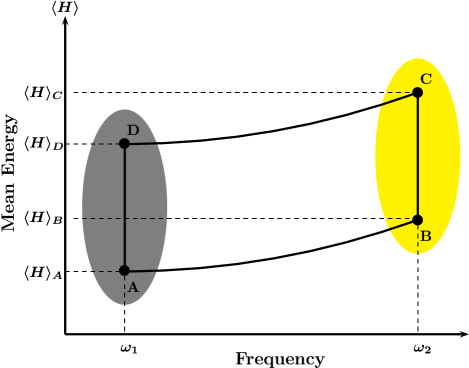
Figure 1: Model of quantum Otto Cycle employing time-dependent harmonic oscillator as the working fluid.

The paper is organized as follows. In Sec. II, we discuss the model of HQOC coupled to a hot squeezed thermal reservoir. In Sec. III, we obtain analytic expression for the upper bound on the efficiency of the engine operating in the sudden switch limit. We also obtain analytic expression for the efficiency at maximum work and compare it with the derived upper bound. In Sec. IV, we repeat our analysis for the Otto refrigerator coupled to a cold squeezed reservoir and obtain upper bound on the COP of the refrigerator. We conclude in Sec. V.

II Quantum Otto cycle with squeezed reservoir

We consider quantum Otto cycle of a time-dependent harmonic oscillator coupled to a hot squeezed thermal bath while cold bath is still purely thermal in nature. It consists of four stages: two adiabatic and two isochoric. These processes occur in the following order Abah et al. (2012); Abah and Lutz (2016): (1) Adiabatic compression $A\longrightarrow B$: To begin with, the system is at inverse temperature $\beta_{1}$. The system is isolated and frequency of the oscillator is increased from $\omega_{1}$ to $\omega_{2}$. Work is done on the system in this stage. The evolution is unitary and von Neumann entropy of the system remains constant. (2) Hot isochore $B\longrightarrow C$: During this stage, the oscillator is coupled to the squeezed thermal heat reservoir at inverse temperature $\beta_{2}$ at fixed frequency ($\omega_{2}$) and allowed to thermalize. No work is done in this stage, only heat exchange between the system and reservoir takes place. After the completion of the hot isochoric stage, the system relaxes to a nondisplaced squeezed thermal state Kim et al. (2989); Marian and Marian (1993) with mean photon number $\langle n(\beta_{2},r)\rangle=\langle n\rangle+(2\langle n\rangle+1)\sinh^{2}r$, where $r$ is the squeezing parameter and $\langle n\rangle=1/(e^{\beta_{2}\omega_{2}}-1)$ is the thermal occupation number (we have set $\hbar=k_{B}=1$ for simplicity). (3) Adiabatic expansion $C\longrightarrow D$: The system is isolated and the frequency of the oscillator is unitarily decreased back to its initial value $\omega_{1}$. Work is done by the system in this stage. (4) Cold isochore $D\longrightarrow A$: To bring back the working fluid to its initial state, the system is coupled to the cold reservoir at inverse temperature $\beta_{1}$ ($\beta_{1}>\beta_{2}$), and allowed to relax back to the initial thermal state $A$.

The average energies $\langle H\rangle$ of the oscillator at the four stages of the cycle read as follows Roßnagel et al. (2014):

$$\langle H\rangle_{A}=\frac{\omega_{1}}{2}\text{coth}\Big{(}\frac{\beta_{1}\omega_{1}}{2}\Big{)},$$ (1)

$$\langle H\rangle_{B}=\frac{\omega_{2}}{2}\lambda\text{coth}\Big{(}\frac{\beta_{1}\omega_{1}}{2}\Big{)},$$ (2)

$$\langle H_{C}\rangle=\frac{\omega_{2}}{2}\coth\left(\frac{\beta_{2}\omega_{2}}{2}\right)\Delta H(r),$$ (3)

$$\langle H_{D}\rangle=\frac{\omega_{1}}{2}\lambda\coth\left(\frac{\beta_{2}\omega_{2}}{2}\right)\Delta H(r),$$ (4)

where $\Delta H(r)=\langle n(\beta_{2},r)\rangle/\langle n\rangle=1+(2+1/\langle n\rangle)\sinh^{2}r$ reflects the effect of the squeezed hot thermal bath on the mean energy of the oscillator, $\lambda$ is the dimensionless adiabaticity parameter Husimi (1953). For the adiabatic process, $\lambda=1$; for non-adiabatic expansion and compression strokes, $\lambda>1$. The expression for mean heat exchanged during the hot and cold isochores can be evaluated, respectively, as follows:

$$\langle Q_{2}\rangle = \langle H\rangle_{C}-\langle H\rangle_{B}$$

$$= \frac{\omega_{2}}{2}\Big{[}\Delta H(r)\text{coth}\Big{(}\frac{\beta_{2}\omega_{2}}{2}\Big{)}-\lambda\text{coth}\Big{(}\frac{\beta_{1}\omega_{1}}{2}\Big{)}\Big{]},$$

(5)

$$\langle Q_{4}\rangle = \langle H\rangle_{A}-\langle H\rangle_{D}$$

$$= \frac{\omega_{1}}{2}\Big{[}\text{coth}\Big{(}\frac{\beta_{1}\omega_{1}}{2}\Big{)}-\lambda\Delta H(r)\text{coth}\Big{(}\frac{\beta_{2}\omega_{2}}{2}\Big{)}\Big{]}.$$

Here, we are employing a sign convention in which heat absorbed (rejected) from (to) the reservoir is positive (negative) and work done on (by) the system is positive (negative).

Since after one complete cycle, the working fluid comes back to its initial state, the extracted work in one complete cycle is given by, $\langle W_{\rm ext}\rangle=\langle Q_{2}\rangle+\langle Q_{4}\rangle>0$. In this work, we are interested in the sudden switch case for which $\lambda=(\omega_{1}^{2}+\omega_{2}^{2})/2\omega_{1}\omega_{2}$ Husimi (1953); Deffner and Lutz (2008); Deffner et al. (2010). Substituting above expression for $\lambda$ in Eqs. (5) and (LABEL:heat4), we obtain the following expressions for the extracted work, $\langle W_{\rm ext}\rangle$, and efficiency, $\eta=\langle W_{\rm ext}\rangle/\langle Q_{2}\rangle$, of the engine, respectively:

$$\langle W_{\rm ext}\rangle=\langle Q_{2}\rangle+\langle Q_{4}\rangle=\frac{\omega_{2}^{2}-\omega_{1}^{2}}{4\omega_{1}\omega_{2}}\left[\omega_{1}\Delta H(r)\coth\left(\frac{\beta_{2}\omega_{2}}{2}\right)-\omega_{2}\coth\left(\frac{\beta_{1}\omega_{1}}{2}\right)\right],$$ (7)

$$\eta=\frac{\langle W_{\rm ext}\rangle}{\langle Q_{2}\rangle}=\left[\frac{2}{1-\frac{\omega_{1}^{2}}{\omega_{2}^{2}}}+\frac{1}{\frac{\omega_{1}}{\omega_{2}}\Delta H(r)\coth\big{(}\frac{\beta_{2}\omega_{2}}{2}\big{)}\tanh\big{(}\frac{\beta_{1}\omega_{1}}{2}\big{)}-1}\right]^{-1}.$$ (8)

Now, efficiency, $\eta$, can attain its maximum when the expression inside the square bracket attains its minimum value. The minimum value of the first term can be inferred as follows: $Min[A_{1}]\equiv Min[2/(1-\omega_{1}^{2}/\omega_{2}^{2})]=2$, as $\omega_{1}<\omega_{2}$ for the engine operation. Similarly, $Min[A_{2}]\equiv Min[1/\{\frac{\omega_{1}}{\omega_{2}}\Delta H(r)\coth(\beta_{2}\omega_{2}/2)\tanh(\beta_{1}\omega_{1}/2)-1\}]=0$, which can be inferred from the positive work condition, $\langle W_{\rm ext}\rangle>0$ [see Eq. (7)], which implies that $\frac{\omega_{1}}{\omega_{2}}\Delta H(r)\coth(\beta_{2}\omega_{2}/2)\tanh(\beta_{1}\omega_{1}/2)>1$. Thus, we can conclude that the efficiency of a harmonic quantum Otto engine, operating in the sudden switch limit, is bounded from above by one-half the unit value, i.e.,

$$\eta\leq\frac{1}{2}\equiv\eta_{\rm max}.$$ (9)

This is our first main result. The result is very interesting as it implies that even in the presence of very very large squeezing ($r\rightarrow\infty$), the efficiency of the engine can never surpass 1/2. This is in contrast with the previous studies, valid for the quasi-static regime, implying that the thermal engine fueled by a hot squeezed thermal reservoir asymptotically attains unit efficiency for large squeezing parameter ($r>>1$) Roßnagel et al. (2014); Manzano et al. (2016); Niedenzu et al. (2018). We attribute this to the highly frictional nature of the sudden switch regime as explained below. In the sudden switch regime, the sudden quench of the frequency of the harmonic oscillator induces non-adiabatic transitions between its energy levels, thereby causing the system to develop coherence in the energy frame. In such a case, the energy entropy increases and an additional parasitic internal energy is stored in the working medium. The additional energy corresponds to the waste (or excess) heat which is dissipated to the heat reservoirs during the proceeding isochoric stages of the cycle Rezek (2010); Plastina et al. (2014). This limits the performance of the device under consideration.

III Upper bound on the efficiency

In order to obtain analytic expression in closed form for the efficiency, we will work in the high-temperature regime Kosloff (1984); Uzdin and Kosloff (2014); Singh and Johal (2019). In this regime, we set $\coth(\beta_{i}\omega_{i}/2)\approx 2/(\beta_{i}\omega_{i})$ ($i=1,2$) and $\Delta H(r)=\cosh(2r)$. Then, the expressions for the extracted work $\langle W_{\rm ext}\rangle$ [Eq. (7)] and the efficiency [Eq. (8)] take the following forms:

$$\langle W_{\rm ext}\rangle = \frac{(1-z^{2})\left[z^{2}\cosh(2r)-\tau\right]}{2z^{2}\beta_{2}},$$ (10)

$$\eta = \frac{(z^{2}-1)[z^{2}\cosh(2r)-\tau]}{\tau-z^{2}[2\cosh(2r)-\tau]},$$ (11)

where we have defined $z=\omega_{1}/\omega_{2}$ and $\tau=\beta_{2}/\beta_{1}=1-\eta_{C}$. From Eq. (10), the positive work condition, $\langle W_{\rm ext}\rangle>0$, implies that

$$z^{2}\cosh(2r)>1-\eta_{C}.$$ (12)

Using the expression for efficiency in Eq. (11), $z^{2}$ can be written in terms of $\eta$ and $\eta_{C}$, and is given by

$$z^{2}=\frac{1}{2}\left\{(1-\eta_{c})(1+\eta)+(1-2\eta)\cosh(2r)-\sqrt{\big{[}(1-\eta_{c})(1+\eta)+(1-2\eta)\cosh(2r)\big{]}^{2}-4(1-\eta_{c})(1+\eta)\cosh(2r)}\right\}.$$ (13)

Using the above expression for $z$ in Eq. (12), we obtain following upper bound on the efficiency of the engine:

$$\eta<\frac{\left[1-\eta_{C}-\cosh(2r)\right]\left[-1+\eta_{C}-2\cosh(2r)+2\sqrt{2\left[1-\eta_{C}\right]\cosh(2r)}\right]}{\left[1-\eta_{C}-2\cosh(2r)\right]{}^{2}}\equiv\eta_{\rm up}.$$ (14)

This is our second main result. Notice that the above derived bound is independent of the parameters of the model under consideration and depends on the reservoir parameters $r$ and $\eta_{C}$ (or $\tau$) only. For $r\rightarrow\infty$, $\eta_{\rm up}\rightarrow 1/2$, which reconfirms our earlier result [Eq. (9)] that the maximum efficiency that our engine can attain is one-half the unit efficiency; it never reaches unit efficiency unlike the engines operating in the quasi-static regime Roßnagel et al. (2014); Manzano et al. (2016); Niedenzu et al. (2018).

Further, we derive analytic expression for the efficiency at maximum work by optimizing Eq. (10) with respect to $z$, and it is given by:

$$\eta_{\rm MW}=\frac{1-\sqrt{(1-\eta_{C})\operatorname{sech}(2r)}}{2+\sqrt{(1-\eta_{C})\operatorname{sech}(2r)}}.$$ (15)

We have plotted Eqs. (14) and (15) in Fig. 2 as a function of $r$ for different fixed values of Carnot efficiency $\eta_{C}$. For the given values of $\eta_{C}$ smaller than 1/2, both $\eta_{\rm up}$ (solid red and blue curves) and $\eta_{\rm MW}$ (dashed red and blue curves) can surpass corresponding Carnot efficiency (dotted curves with same color) for some value of squeezing parameter $r$ and approach 1/2 for relatively larger values of $r\,(r>5)$. From the inset of Fig. 2, it is clear that $\eta_{\rm MW}$ always lies below $\eta_{\rm up}$, which should be the case as for the given temperature ratio ($\eta_{C}$), $\eta_{\rm up}$ is the upper bound on the efficiency.

One more comment is in order here. Although, for given values of $\eta_{C}$ ($\eta_{C}<1/2$), $\eta_{\rm up}$ and $\eta_{\rm MW}$ may surpass standard Carnot efficiency, they can never surpass generalized Carnot efficiency (not shown in Fig. 2) Alicki (2014); Roßnagel et al. (2014),

$$\eta^{\rm gen}_{C}=1-\frac{\beta_{2}}{\beta_{1}\cosh(2r)}\equiv 1-\frac{T_{1}}{T_{2}\cosh(2r)},$$ (16)

which follows from the second law of thermodynamics applied to the nonequilibrium situations Abah and Lutz (2014). The concept of generalized Carnot efficiency can be understood as follows. We can always assign a frequency dependent local temperature to a squeezed thermal reservoir characterized by its genuine temperature $T$ and squeezing parameter $r$ Alicki (2014); Alicki and Gelbwaser-Klimovsky (2015). The expression for this frequency dependent local temperature can be obtained from the following relation Alicki (2014); Alicki and Gelbwaser-Klimovsky (2015):

$$\exp\left(-\frac{\omega}{T(\omega,r)}\right)=\frac{\langle n\rangle+(2\langle n\rangle+1)\sinh^{2}r}{1+\langle n\rangle+(2\langle n\rangle+1)\sinh^{2}r}.$$ (17)

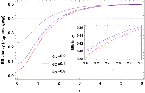
Figure 2: Plots of $\eta_{\rm up}$ [Eq. (14)] and $\eta_{\rm MW}$ [Eq. (15)] as a function of squeezing parameter $r$. Solid red and blue curves represent $\eta_{\rm up}$ for $\eta_{C}=0.2$ and $\eta_{C}=0.4$, respectively. Dashed curves in the corresponding color represent $\eta_{\rm MW}$. Dotted red and blue curves denote the standard Carnot efficiency at values $\eta_{C}=0.2$ and $\eta_{C}=0.4$, respectively. Solid purple curve represent $\eta_{\rm up}$ for $\eta_{C}=0.8$, and shows that for the given value of $\eta_{C}>1/2$, $\eta_{\rm up}$ can never surpass Carnot efficiency $\eta_{C}$ even in the presence of very large squeezing. For the better resolution, in the inset, we have plotted $\eta_{\rm up}$ and $\eta_{\rm MW}$ for smaller range of $r$. It shows that for the same value of squeezing parameter $r$, $\eta_{\rm MW}$ always lies below $\eta_{\rm up}$.

In the high-temperature limit, the effective temperature of the squeezed hot bath reads as,

$$T^{\rm eff}_{2}(r)=T_{2}(1+2\sinh^{2}r)=T_{2}\cosh(2r).$$ (18)

Hence, for positive values of $r$, engine may be assumed to be operating between temperatures $T_{1}$ and $T^{\rm eff}_{2}(r)$. The actual (generalized) Carnot efficiency should then be given by Eq. (16).

Finally, we discuss the special case when $r\rightarrow 0$. This corresponds to the case in which our harmonic quantum engine is working between two purely thermal reservoirs. Thus, for $r\rightarrow 0$, Eqs. (14) and (15) reduce to the following forms, respectively:

$$\eta<\frac{[3-2\sqrt{2(1-\eta_{C})}-\eta_{C}]\eta_{C}}{(1+\eta_{C})^{2}}\equiv\eta^{\rm th}_{\rm up},$$ (19)

$$\eta_{\rm RK}=\frac{1-\sqrt{1-\eta_{C}}}{2+\sqrt{1-\eta_{C}}}.$$ (20)

The above bound, $\eta^{\rm th}_{\rm up}$, is much tighter than the classical Carnot bound, even tighter than $\eta_{C}/2$ (see Fig. 3). Eq. (20), which we derived as a special case of our more general result Eq. (14), was first derived by Rezek and Kosloff (RK) for the optimization of a harmonic quantum Otto engine undergoing sudden switch of frequencies in the adiabatic stages Rezek and Kosloff (2006). Again, it is clear from Fig. 3 that $\eta_{\rm RK}$ (dashed red curve) always lies below $\eta^{\rm th}_{\rm up}$ (solid blue curve), which should be the case.

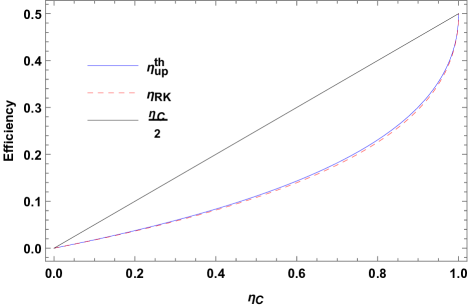
Figure 3: Plots of $\eta^{\rm th}_{\rm up}$ [Eq. (19)], $\eta_{\rm RK}$ [Eq. (20)] versus Carnot efficiency. We can see that $\eta_{\rm RK}$ (dashed red curve) lies below $\eta^{\rm th}_{\rm up}$ (solid blue curve). Both are bounded above by half the Carnot efficiency, $\eta_{C}/2$.

IV Upper bound on the coefficient of performance

Here, we discuss the operation of QHOC as a refrigerator. In the refrigeration process, heat is absorbed from the cold bath, $\langle Q_{4}\rangle>0$, and dumped into the hot bath, $\langle Q_{2}\rangle<0$. The net work investigated in the system is positive, $\langle W_{\rm in}\rangle=-(\langle Q_{2}\rangle+\langle Q_{4}\rangle)>0$. Here, we will first discuss the case when refrigerator is coupled to two purely thermal reservoirs. We follow the same procedure as done for the heat engine in Sec. III. Since the calculations are straight forward, we merely present our results here. For the refrigerator running between two purely thermal reservoirs, positive cooling condition, $\langle Q_{4}\rangle>0$, implies that

$$\zeta_{C}>1\quad\text{\rm and}\quad\zeta\leq 1+3\zeta_{C}-2\sqrt{2\zeta(1+\zeta_{C})}\equiv\zeta^{\rm th}_{\rm up},$$ (21)

where $\zeta=\omega_{1}/(\omega_{2}-\omega_{1})$ and $\zeta_{C}=\beta_{2}/(\beta_{1}-\beta_{2})$ are the COP and Carnot COP, respectively. The condition $\zeta_{C}>1$ implies that $\tau>1/2$, which in turns implies that cold reservoir cannot be cooled below the temperature $T_{2}/2$, thus putting a restriction to the operation of the refrigerator operating in sudden-switch regime. The upper bound $\zeta_{\rm up}$ derived here is independent of the parameters of the system and depends on ratio of the reservoir temperatures only, which makes it quite general in nature. Similar to the heat engine case, the obtained upper bound is much tighter than the corresponding Carnot bound.

Now, we will discuss the effect of coupling the refrigerator to the cold squeezed reservoir. In the high-temperature regime, the mean energies at points $A$, $B$, $C$ and $D$ are given by: $\langle H\rangle_{A}=\omega_{1}\coth(\beta_{1}\omega_{1}/2)\cosh(2r)/2$, $\langle H\rangle_{B}=\omega_{2}\lambda\coth(\beta_{1}\omega_{1}/2)\cosh(2r)/2$, $\langle H\rangle_{C}=\omega_{2}\coth(\beta_{2}\omega_{2}/2)$, $\langle H\rangle_{D}=\omega_{1}\lambda\coth(\beta_{2}\omega_{2}/2)/2$. The positive cooling condition, $\langle Q_{4}\rangle>0$, yields the following expressions:

$$\frac{1}{2}\text{sech}(2r)<\tau<\text{sech}(2r)\quad\text{and}\quad\zeta<\frac{3}{1-\tau\cosh(2r)}-2-2\sqrt{2}\sqrt{\frac{\tau\cosh(2r)}{(\tau\cosh(2r)-1)^{2}}}\equiv\zeta_{up}.$$ (22)

Eq. (22) along with the equation (21) is our third main result. As expected, $\zeta_{\rm up}$ reduces to $\zeta^{\rm th}_{up}$ for the vanishing squeezing parameter, $r=0$. To discuss the physical significance of condition given in Eq. (22), we invert it in terms of lower and upper limits on squeezing parameter $r$:

$$0<\tau<\frac{1}{2},\quad\frac{1}{2}\cosh^{-1}\left(\frac{1}{2\tau}\right)<r<\frac{1}{2}\cosh^{-1}\left(\frac{1}{\tau}\right)\quad\text{or}\quad\frac{1}{2}<\tau<1,\quad 0<r<\frac{1}{2}\cosh^{-1}\left(\frac{1}{\tau}\right).$$ (23)

It is clear from the above equation that we can extract heat from squeezed cold reservoir even for $\tau<1/2$, which is otherwise impossible with the refrigeration operation with purely thermal reservoirs. Again this can be explained on the basis of effective temperature of the cold reservoir [see Eq. (18)]. For $r=\frac{1}{2}\cosh^{-1}\left(\frac{1}{2\tau}\right)$ and $r=\frac{1}{2}\cosh^{-1}\left(\frac{1}{\tau}\right)$, the effective temperatures of the cold reservoir become $T_{2}/2$ and $T_{2}$, respectively. As per the original positive work condition ($1/2<\tau$) without cold squeezed reservoir, $T_{1}>T_{2}/2$, hence in case of cold squeezed reservoir this condition is satisfied for the given range of squeezing parameter $r$ in Eq. (23). Eventually, the refrigeration stops when effective temperature of cold squeezed reservoir approaches $T_{2}$, which is temperature of the thermal hot reservoir. Finally, for $\tau=1/2$ or $T_{2}=2T_{1}$, the allowed range of $r$ is: $0<r<\frac{1}{2}\cosh^{-1}(2)$, which implies that effective temperature of cold reservoir should be smaller than $2T_{1}$ which is natural.

V Conclusions

We have investigated the performance of a HQOC, operating in the sudden switch limit, coupled to a squeezed thermal reservoir. First, we showed that even in the presence of very large squeezing ($r\rightarrow\infty$), the maximum efficiency of the engine is 1/2 only. This is due to the frictional effects caused by the non-adiabatic transitions when we operate in the sudden switch regime. Our study is in contrast with the previous studies which claim that the efficiency can reach unity for large squeezing. Then we obtained closed form expression for the upper bound on the efficiency of the engine operating in the high-temperature regime. The result is interesting in the sense that the obtained bound is independent of the parameters of the model under consideration and depends on the ratio of the reservoir temperatures and squeezing parameter $r$ only. Additionally, we also derive the analytic expression for the efficiency at maximum work and showed that it satisfies the derived upper bound. As a special case of our more general setup, when squeezing parameter $r\rightarrow 0$, our results correspond to the case in which engine is running between two purely thermal reservoirs. Further, we have also obtained upper bounds for the Otto refrigerator working between two purely thermal reservoirs as well as for the case when cold reservoir is taken to be squeezed thermal reservoir. Finally, we showed that squeezing can help in cooling process otherwise impossible in standard setup with thermal reservoirs.

References

- Kondepudi and Prigogine (2014) D. Kondepudi and I. Prigogine, Modern thermodynamics: from heat engines to dissipative structures (John Wiley & Sons, 2014).
- Vinjanampathy and Anders (2016) S. Vinjanampathy and J. Anders, Contemp. Phys. 57, 545 (2016).
- Mahler (2014) G. Mahler, Quantum thermodynamic processes: Energy and information flow at the nanoscale (Jenny Stanford Publishing, 2014).
- Deffner and Campbell (2019) S. Deffner and S. Campbell, Quantum Thermodynamics (Morgan & Claypool Publishers, 2019).
- Alicki and Kosloff (2018) R. Alicki and R. Kosloff, in Thermodynamics in the Quantum Regime (Springer, 2018) pp. 1–33.
- Scully (2001) M. O. Scully, Phys. Rev. Lett. 87, 220601 (2001).
- Scully et al. (2003) M. O. Scully, M. S. Zubairy, G. S. Agarwal, and H. Walther, Science 299, 862 (2003).
- Türkpençe and Müstecaplıoğlu (2016) D. Türkpençe and O. E. Müstecaplıoğlu, Phys. Rev. E 93, 012145 (2016).
- Skrzypczyk et al. (2014) P. Skrzypczyk, A. J. Short, and S. Popescu, Nat. Commun. 5, 4185 (2014).
- Bera et al. (2017) M. N. Bera, A. Riera, M. Lewenstein, and A. Winter, Nat. Commun. 8, 1 (2017).
- Park et al. (2013) J. J. Park, K.-H. Kim, T. Sagawa, and S. W. Kim, Phys. Rev. Lett. 111, 230402 (2013).
- Brunner et al. (2014) N. Brunner, M. Huber, N. Linden, S. Popescu, R. Silva, and P. Skrzypczyk, Phys. Rev. E 89, 032115 (2014).
- Perarnau-Llobet et al. (2015) M. Perarnau-Llobet, K. V. Hovhannisyan, M. Huber, P. Skrzypczyk, N. Brunner, and A. Acín, Phys. Rev. X 5, 041011 (2015).
- Altintas et al. (2014) F. Altintas, A. U. C. Hardal, and O. E. Müstecaplıoğlu, Phys. Rev. E 90, 032102 (2014).
- Roßnagel et al. (2014) J. Roßnagel, O. Abah, F. Schmidt-Kaler, K. Singer, and E. Lutz, Phys. Rev. Lett. 112, 030602 (2014).
- Huang et al. (2012) X. L. Huang, T. Wang, and X. X. Yi, Phys. Rev. E 86, 051105 (2012).
- Kosloff and Rezek (2017) R. Kosloff and Y. Rezek, Entropy 19, 136 (2017).
- Agarwalla et al. (2017) B. K. Agarwalla, J.-H. Jiang, and D. Segal, Phys. Rev. B 96, 104304 (2017).
- Manzano et al. (2016) G. Manzano, F. Galve, R. Zambrini, and J. M. Parrondo, Phys. Rev. E 93, 052120 (2016).
- Xiao and Li (2018) B. Xiao and R. Li, Phys. Lett. A 382, 3051 (2018).
- Long and Liu (2015) R. Long and W. Liu, Phys. Rev. E 91, 062137 (2015).
- Klaers et al. (2017) J. Klaers, S. Faelt, A. Imamoglu, and E. Togan, Phys. Rev. X 7, 031044 (2017).
- Correa et al. (2014) L. A. Correa, J. P. Palao, D. Alonso, and G. Adesso, Sci. Rep. 4, 3949 (2014).
- de Assis et al. (2020) R. J. de Assis, J. Sales, U. C. Mendes, and N. G. de Almeida, arXiv:2003.12664 (2020).
- Wang et al. (2019) J. Wang, J. He, and Y. Ma, Phys. Rev. E 100, 052126 (2019).
- Niedenzu et al. (2018) W. Niedenzu, V. Mukherjee, A. Ghosh, A. G. Kofman, and G. Kurizki, Nat. Commun. 9, 1 (2018).
- Abah and Lutz (2014) O. Abah and E. Lutz, EPL (Europhysics Letters) 106, 20001 (2014).
- Niedenzu et al. (2016) W. Niedenzu, D. Gelbwaser-Klimovsky, A. G. Kofman, and G. Kurizki, New J. Phys. 18, 083012 (2016).
- Alicki and Gelbwaser-Klimovsky (2015) R. Alicki and D. Gelbwaser-Klimovsky, New J. Phys. 17, 115012 (2015).
- Alicki (2014) R. Alicki, arXiv:1401.7865 (2014).
- Ghosh et al. (2018) A. Ghosh, D. Gelbwaser-Klimovsky, W. Niedenzu, A. I. Lvovsky, I. Mazets, M. O. Scully, and G. Kurizki, Proc. Natl. Acad. Sci. USA 115, 9941 (2018).
- Manzano (2018) G. Manzano, Phys. Rev. E 98, 042123 (2018).
- Quan et al. (2007) H. T. Quan, Y.-x. Liu, C. P. Sun, and F. Nori, Phys. Rev. E 76, 031105 (2007).
- Kieu (2004) T. D. Kieu, Phys. Rev. Lett. 93, 140403 (2004).
- Rezek and Kosloff (2006) Y. Rezek and R. Kosloff, New J. Phys. 8, 83 (2006).
- Abah et al. (2012) O. Abah, J. Roßnagel, G. Jacob, S. Deffner, F. Schmidt-Kaler, K. Singer, and E. Lutz, Phys. Rev. Lett. 109, 203006 (2012).
- Thomas and Johal (2011) G. Thomas and R. S. Johal, Phys. Rev. E 83, 031135 (2011).
- Chand and Biswas (2017) S. Chand and A. Biswas, EPL (Europhysics Letters) , 60003 (2017).
- Peterson et al. (2019) J. P. Peterson, T. B. Batalhão, M. Herrera, A. M. Souza, R. S. Sarthour, I. S. Oliveira, and R. M. Serra, Phys. Rev. Lett. 123, 240601 (2019).
- Abah and Lutz (2016) O. Abah and E. Lutz, EPL (Europhysics Letters) 113, 60002 (2016).
- Kim et al. (2989) M. Kim, F. De Oliveira, and P. Knight, Phys. Rev. A 40, 2494 (2989).
- Marian and Marian (1993) P. Marian and T. A. Marian, Phys. Rev. A 47, 4474 (1993).
- Husimi (1953) K. Husimi, Prog. Theor. Exp. Phys. 9, 238 (1953).
- Deffner and Lutz (2008) S. Deffner and E. Lutz, Phys. Rev. E 77, 021128 (2008).
- Deffner et al. (2010) S. Deffner, O. Abah, and E. Lutz, Chem. Phys. 375, 200 (2010).
- Rezek (2010) Y. Rezek, Entropy 12, 1885 (2010).
- Plastina et al. (2014) F. Plastina, A. Alecce, T. J. Apollaro, G. Falcone, G. Francica, F. Galve, N. L. Gullo, and R. Zambrini, Phys. Rev. Lett. 113, 260601 (2014).
- Kosloff (1984) R. Kosloff, J. Chem. Phys. 80, 1625 (1984).
- Uzdin and Kosloff (2014) R. Uzdin and R. Kosloff, EPL (Europhysics Letters) 108, 40001 (2014).
- Singh and Johal (2019) V. Singh and R. S. Johal, Phys. Rev. E 100, 012138 (2019).