Efficient Algorithms for Convolutional Inverse Problems in Multidimensional Imaging

Abstract

Multidimensional imaging, capturing image data in more than two dimensions, has been an emerging field with diverse applications. Due to the limitation of two-dimensional detectors in obtaining the high-dimensional image data, computational imaging approaches have been developed to pass on some of the burden to a reconstruction algorithm. In various image reconstruction problems in multidimensional imaging, the measurements are in the form of superimposed convolutions. In this paper, we introduce a general framework for the solution of these problems, called here convolutional inverse problems, and develop fast image reconstruction algorithms with analysis and synthesis priors. These include sparsifying transforms, as well as convolutional or patch-based dictionaries that can adapt to correlations in different dimensions. The resulting optimization problems are solved via alternating direction method of multipliers with closed-form, efficient, and parallelizable update steps. To illustrate their utility and versatility, the developed algorithms are applied to three-dimensional image reconstruction problems in computational spectral imaging for cases with or without correlation along the third dimension. As the advent of multidimensional imaging modalities expands to perform sophisticated tasks, these algorithms are essential for fast iterative reconstruction in various large-scale problems.

Keywords multidimensional imaging  $\cdot$ convolutional inverse problems  $\cdot$ sparse recovery  $\cdot$ convolutional dictionary

1 Introduction

Multidimensional imaging, that is, capturing image data in more than two dimensions, has been a prominent field with ubiquitous applications in the physical and life sciences [1, 2]. The multidimensional image data, including the spatial, spectral, and temporal distributions of light (or an electromagnetic field), provide unprecedented information about the chemical, physical, and biological properties of targeted scenes [1, 2, 3, 4, 5].

While the objective of conventional photography is to measure only the two-dimensional spatial distribution of light, the objective of multidimensional imaging is to form images of a radiating scene as a function of more than two variables. That is, the goal is to obtain a datacube of high dimensions, for example, in three spatial coordinates $(x,y,z)$, wavelength $(\lambda)$ and time $(t)$. However, obtaining this high-dimensional image data with inherently two-dimensional detectors poses intrinsic limitations on the spatio-spectral-temporal extent of these techniques.

Conventional techniques circumvent this limitation by sequential scanning of a series of two-dimensional measurements to form the high-dimensional image data. For example, in spectral imaging, the three-dimensional datacube $(x,y,\lambda)$ is typically obtained by either using a spectrometer with a long slit and scanning the scene spatially, or by using an imager with a series of spectral filters and scanning the scene spectrally.

As a result, these scanning-based conventional methods generally suffer from low signal-to-noise ratio (SNR), high acquisition time, and temporal artifacts for dynamic scenes. Moreover, the attainable resolutions (such as temporal, spatial, and spectral) are inherently limited by the physical components involved.

To overcome these drawbacks, computational imaging approaches have been developed to pass on some of the burden to a reconstruction algorithm [2, 4, 6, 5, 7]. In these approaches, image data is reconstructed by combining information from multiplexed measurements with the additional prior (statistical or structural) knowledge about the unknown image.

In many image reconstruction problems in multidimensional imaging, the measurements are in the form of superimposed convolutions. That is, the relationship between the measured (sensor) data and the unknown images can often be adequately characterized by sum of multiple convolutions. In fact, for linear shift-variant systems whose response slowly varies across the field of view, time, depth, or spectral dimensions, the system operator can often be approximated by a linear combination of regular convolution operators [8, 9]. In this paper, we focus on the solution of this type of inverse problems, which are called here convolutional inverse problems [10]. Such inverse problems are encountered in various computational imaging modalities such as computational photography, wide-field astronomical imaging, three-dimensional microscopy, spectral imaging, ultrafast imaging, radio interferometric imaging, magnetic resonance imaging, and ultrasound imaging [10, 5, 6, 7, 11, 9, 8, 12, 13, 14, 15, 16, 17, 18, 19].

In this paper, we introduce a unified framework for the solution of convolutional inverse problems by considering a general image-formation model. Based on alternating direction method of multipliers (ADMM) [20], we develop fast image reconstruction algorithms that can exploit sparse models in analysis or synthesis forms for the high-dimensional image data, as well as correlations in different dimensions. In the analysis case, multidimensional discrete derivative operators or sparsifying transforms can be utilized such as discrete cosine transform (DCT), wavelets, or their Kronecker-product forms [21, 5, 7]. In the synthesis case, convolutional or patch-based dictionaries can be utilized, which can also be adapted to correlations in different dimensions [10, 22, 23, 24, 25, 26, 27, 28, 29, 30, 31]. Based on the available prior knowledge about the image of interest, there may be correlations either all through the image data or only in certain dimensions. The inverse problem is formulated for both cases and the resulting optimization problems are solved via ADMM. The obtained reconstruction algorithms have closed-form, efficient, and parallelizable update steps. To illustrate their utility and versatility, these algorithms are applied to three-dimensional (3D) reconstruction problems in computational spectral imaging, and their performance is numerically demonstrated for various cases with or without correlation along the third dimension.

ADMM-based reconstruction algorithms have been earlier developed for certain multidimensional imaging modalities with specific prior and observation models [5, 7]. To the best of our knowledge, convolutional inverse problems have not been studied with this generality considering different correlation and prior models. A multidimensional signal of interest may or may not be correlated in all directions, which accordingly determines the dimension of the transforms/dictionaries used in these models (for example, 2D or 3D) and the reconstruction approach. The versatile ADMM-based reconstruction algorithms developed in this paper are powerful in that they can be applied to various imaging modalities involving convolutional inverse problems.

This paper is organized as follows. In Section II, we introduce the convolutional measurement model. The convolutional inverse problem is then formulated in Section III using different priors. Section IV provides the details of the developed image reconstruction algorithms and explains their efficient implementation for cases with correlations all through the image data or only in certain dimensions. Numerical simulation results for three-dimensional reconstruction problems in computational spectral imaging are presented in Section V. Section VI concludes the paper and discusses the future directions.

2 Forward Problem

In many image reconstruction problems in multidimensional imaging, the measurements can be modeled in the following form of superimposed convolutions:

$${y_{k}[n_{1},n_{2}]}=\sum_{s=1}^{S}{x_{s}[n_{1},n_{2}]*h_{k,s}[n_{1},n_{2}]}+{w_{k}[n_{1},n_{2}]},$$ (1)

where the measurement index $k$ = $1,\ldots,K$. This is a general multiple-input multiple-output model, where ${y_{k}}$’s denote the different 2D measurements and ${x_{s}}$’s represent the 2D slices of the unknown image to be reconstructed. Hence, each measurement ${y_{k}}$ consists of blurred and superimposed images of ${x_{s}}$’s. We assume that the size of the measurements and the slices of the unknown image are both limited to $N\times N$. Here, ${h_{k,s}}$ denotes the blur function (point-spread function) acting on the $s$th image slice, ${x_{s}}$, in the $k$th measurement, ${y_{k}}$. These blur functions generally model the slowly varying response of a shift-variant imaging system across the dimensions of time, space, spectral, depth, and such.

This general forward model involving sum of convolutions is encountered in many imaging problems such as different three-dimensional image reconstruction problems ($K\geq 1$, $S\geq 1$) in computational imaging [9, 8, 11, 12, 13, 14, 15, 16, 17, 18, 19], as well as classical and multiframe image deconvolution ($K\geq 1$, $S=1$). Note that our model allows each blurring operator to have a different weight as commonly used in the literature; for simplicity, these weights are simply embedded into the terms ${h_{k,s}}$’s in our model.

Using lexicographic ordering and linearity of the convolution operator, the model in Eq. (1) can be cast in the following matrix-vector form:

$$\mathbf{y}_{k}=\sum_{s=1}^{S}\mathbf{H}_{k,s}\mathbf{x}_{s}+\mathbf{w}_{k}.$$ (2)

Here, $\mathbf{y}_{k}\in\mathbb{R}^{N^{2}}$ represents the noisy ${k}$th measurement vector, $\mathbf{x}_{s}\in\mathbb{R}^{N^{2}}$ denotes the vector for the $s$th image slice, and $\mathbf{H}_{k,s}\in\mathbb{R}^{N^{2}\times N^{2}}$ is the convolution matrix representing the convolution with the blur function ${h_{k,s}}$. Lastly, $\mathbf{w}_{k}$ denotes the white Gaussian noise vector whose each entry has mean zero and variance $\sigma^{2}_{k}$. By concatenating the measurement vectors $\mathbf{y}_{k}$’s and the image slice vectors $\mathbf{x}_{s}$’s vertically, the model in Eq. (2) can be expressed in the following final form:

$$\mathbf{y}=\mathbf{H}\mathbf{{x}}+\mathbf{w},$$ (3)

$$\mathbf{H}=\left(\begin{array}[]{ccc}\mathbf{H}_{1,1}&\cdots&\mathbf{H}_{1,S}\\ \vdots&\ddots&\vdots\\ \mathbf{H}_{K,1}&\cdots&\mathbf{H}_{K,S}\end{array}\right),\mathbf{y}=\left[\begin{array}[]{c}\mathbf{y}_{1}\\ {:}\\ \mathbf{y}_{K}\end{array}\right],\mathbf{x}=\left[\begin{array}[]{c}\mathbf{x}_{1}\\ {:}\\ \mathbf{x}_{S}\end{array}\right]$$

Here $\mathbf{y}\in\mathbb{R}^{KN^{2}}$ is the vertically concatenated measurement vector. Similarly, the vector $\mathbf{x}\in\mathbb{R}^{SN^{2}}$ is the concatenated image vector, which consists of the image slices. The measurement matrix $\mathbf{H}\in\mathbb{R}^{KN^{2}\times SN^{2}}$ contains all the convolution matrices involved. Lastly, the vector $\mathbf{w}$ = $[\mathbf{w}_{1}^{T}\ldots\mathbf{w}_{K}^{T}]^{T}$ denotes the overall noise vector.

3 Convolutional Inverse Problem

In the inverse problem, the goal is to recover the unknown image vector, $\mathbf{x}$, from the noisy measurement vector, $\mathbf{y}$. Because each measurement is composed of blurred images of different slices, the overall task also involves the deconvolution of multiple objects. This convolutional inverse problem is inherently ill-posed, and as the blur functions, $h_{k,s}$, for different slices, $s$, or different measurements, $k$, become similar, the conditioning of the problem gets worse due to the increase in the linear dependency of the columns or rows of $\mathbf{H}$, respectively.

To incorporate the additional prior knowledge about the unknown image vector, this ill-posed inverse problem can be formulated as the following optimization problem:

$$\min_{{\mathbf{x}}}\;\frac{\beta}{2}||\mathbf{y}-\mathbf{H}\mathbf{{x}}||_{2}^{2}+{\cal{R}}(\mathbf{{x}}),$$ (4)

where ${\cal{R}}(\mathbf{{x}})$ is the regularization functional. This regularized least squares problem can also be viewed as a maximum posterior estimation (MAP) problem that exploits statistical priors. Here, the first term controls data fidelity, whereas the second term controls how well the reconstruction matches our prior knowledge of the solution, with the scalar parameter $\beta$ trading off between these two terms.

For regularization, here sparse models in analysis or synthesis forms [21] are exploited. In the analysis case, multidimensional discrete derivative operators or sparsifying transforms such as discrete cosine transform (DCT), wavelets, or their Kronecker-product forms can be utilized [5, 7]. These generally yield fast and efficient computations. In the synthesis case, multidimensional dictionaries can be utilized with local or global sparsity models. One common approach is to partition the image data into patches and represent each local patch in terms of the elements of a small-size dictionary [22, 23, 24]. An alternative approach is to represent the entire image data with a global convolutional dictionary [26]. But there has been limited work for the three or higher dimensional convolutional dictionaries and their performance [29, 30].

Moreover, a multidimensional signal of interest may or may not be correlated in all directions, which consequently determines the dimension of the transform or dictionary used in these sparse models (for example, 3D or 2D). Hence we can also adapt these models to correlations in different dimensions. Here, we formulate the inverse problem for all of these cases.

3.1 Analysis Prior

The analysis prior formulation is given by

$${\cal{R}}(\mathbf{{x}})=\mathbf{\Phi}(\bf{Tx}),$$ (5)

where $\bf{T}$ is a matrix representing an analysis operator such as a multidimensional transform or discrete derivative. For example, for a 3D reconstruction problem, this analysis operator can be a 3D transform if there is correlation all through the image data, or if there is no correlation along the third dimension, the operator can perform a 2D transform along each slice. For the choice of regularization functional $\mathbf{\Phi}(.)$, there are different choices as well. One popular choice is $l_{1}$-norm, i.e. $\mathbf{\Phi}(\mathbf{Tx})=||\mathbf{Tx}||_{1}$. Another common choice is isotropic TV [32], i.e. $\mathbf{\Phi}(\mathbf{Tx})=\rm{TV}(\mathbf{x})$ with $\mathbf{T}$ = $\mathbf{I}$.

3.2 Synthesis Prior

In the synthesis case, the signal $\bf{x}$ is sparsely represented as a linear combination of columns (i.e. atoms) from a dictionary $\bf{\tilde{D}}$. In general, the synthesis prior can be formulated as

$${\cal{R}}(\mathbf{{x}})=\underset{\mathbf{z}}{\min}\;\frac{1}{2}||\bf{\tilde{D}}\mathbf{z}-\mathbf{Px}||^{2}_{2}+\lambda||\mathbf{z}||_{1},$$ (6)

where $\bf{z}$ represents the sparse code. The matrix $\mathbf{P}$ can be either identity or a patch operator depending whether the entire image or its patches are represented. In this work, we consider both patch-based and convolutional dictionaries, which can be learned offline from a training data or online from the measurements through a dictionary update step.

3.2.1 Patch-based Dictionary

Commonly, for efficient computation, a small-size dictionary is used for sparse representation of overlapping image patches. This results in the following prior:

$$\underset{\mathbf{z}_{j}}{\min}\;\sum_{j}\frac{1}{2}||\mathbf{D}\mathbf{z}_{j}-\mathbf{P}_{j}\mathbf{x}||^{2}_{2}+\lambda||\mathbf{z}_{j}||_{1},$$ (7)

where $Q\times Q\times T$ is the patch size and $\mathbf{P}_{j}\in\mathbb{R}^{Q^{2}T\times N^{2}S}$ is the matrix to extract the $j$th patch with $j=1,\ldots,J$. Moreover, $\mathbf{z}_{j}\in\mathbb{R}^{Q^{2}T}$ denotes the sparse code of the $j$th patch and $\mathbf{D}\in\mathbb{R}^{Q^{2}T\times Q^{2}T}$ represents the common dictionary used for all patches. Note that this prior is a special case of the general form given in Eq. (6) where now $\mathbf{P}=[\mathbf{P}_{1}^{T}|\ldots|\mathbf{P}_{J}^{T}]^{T}$ and $\mathbf{\tilde{D}}=\mathbf{I}_{J}\operatorname*{\text{\raisebox{1.07639pt}{\scalebox{0.75}{$\bigotimes$}}}}\mathbf{D}$ with $\operatorname*{\text{\raisebox{1.07639pt}{\scalebox{0.75}{$\bigotimes$}}}}$ denoting the Kronecker product and $\mathbf{I}_{n}$ denoting an identity matrix of size $n\times n$. To adaptively learn the dictionary from the measurements, the prior in Eq. (7) can also be modified as follows:

$$\underset{\mathbf{z}_{j},\mathbf{D}}{\min}\;\sum_{j}\frac{1}{2}||\mathbf{D}\mathbf{z}_{j}-\mathbf{P}_{j}\mathbf{x}||^{2}_{2}+\lambda||\mathbf{z}_{j}||_{1}\;{\text{s.t.}}\;||\mathbf{D}||_{F}=1.$$ (8)

Here, the constraint is needed to avoid the scaling ambiguity of the dictionary.

For an image data with two-dimensional correlations only, the patches can be extracted from each image slice, $\mathbf{x}_{s}$. In this case, there will be an additional summation over image slices in Eq. (7) and (8) with sparse code $\mathbf{z}_{j,s}\in\mathbb{R}^{Q^{2}}$ for the $j$th patch of the $s$th image slice, patch extraction matrix $\mathbf{P}_{j}\in\mathbb{R}^{Q^{2}\times N^{2}}$, dictionary $\mathbf{D}\in\mathbb{R}^{Q^{2}\times Q^{2}}$, and patch size $Q\times Q$.

3.2.2 Convolutional Dictionary

Alternatively, the entire image data can be represented using a global convolutional dictionary [26], hence as a sum of three-dimensional convolutions with a few dictionary filters. This results in the following formulation:

$$\underset{\mathbf{z}_{m}}{\min}\;\frac{1}{2}||\sum_{m}\mathbf{d}_{m}*\mathbf{z}_{m}-\mathbf{x}||^{2}_{2}+\lambda\sum_{m}||\mathbf{z}_{m}||_{1}.$$ (9)

where $\mathbf{d}_{m}\in\mathbb{R}^{L^{2}R}$ is the $m$th dictionary filter of size $L\times L\times R$ and $\mathbf{z}_{m}\in\mathbb{R}^{N^{2}S}$ is the corresponding sparse code of size $N\times N\times S$ with $m=1,\ldots,M$. In this representation, the dictionary size is generally much smaller than the image size (i.e. $L\ll N$ and $R\ll S$), while the sparse code is of the same size as the image. Also note that the dictionary $\mathbf{\tilde{D}}$ in Eq. (6) has a specific form in this case as given by $\mathbf{\tilde{D}}=[\mathbf{D}_{1}\ldots\mathbf{D}_{M}]$ with $\mathbf{D}_{m}$ representing the convolution matrix for the $m$th dictionary filter and $\mathbf{P}$ is identity as the entire image is represented. As before, to adaptively learn the dictionary from the measurements, the prior in Eq. (9) can also be modified as

$$\underset{\mathbf{z}_{m},\mathbf{d}_{m}}{\min} \;\frac{1}{2}||\sum_{m}\mathbf{d}_{m}*\mathbf{z}_{m}-\mathbf{x}||^{2}_{2}+\lambda\sum_{m}||\mathbf{z}_{m}||_{1}$$

s.t. $$\quad||\mathbf{d}_{m}||_{2}=1\quad m=1,2,\ldots,M.$$

For an image data with two-dimensional correlations only, a common convolutional dictionary can be used to represent each image slice, $\mathbf{x}_{s}$, separately. In this case, there will be an additional summation over image slices in Eq. (9) and (3.2.2) with the $m$th dictionary filter $\mathbf{d}_{m}\in\mathbb{R}^{L^{2}}$ of size $L\times L$ and the corresponding sparse code $\mathbf{z}_{m,s}\in\mathbb{R}^{N^{2}}$ for the $s$th image slice.

3.2.3 Convolutional Dictionary with Tikhonov Regularization

Because convolutional dictionaries are known to work well for the representation of high-frequency components of a signal, they are commonly used after highpass filtering [26, 33]. An alternative to this preprocessing is to introduce gradient (Tikhonov) regularization to the sparse code $\mathbf{z}_{m}$’s as follows [34]:

$$\underset{\mathbf{z}_{m}}{\min}\;\frac{1}{2}||\sum_{m}\mathbf{d}_{m}*\mathbf{z}_{m}-\mathbf{x}||^{2}_{2}+\lambda\sum_{m}||\mathbf{z}_{m}||_{1}+$$ (11)

$$\frac{\mu}{2}\sum_{m}||\mathbf{r}_{1}*\mathbf{z}_{m}||^{2}_{2}+||\mathbf{r}_{2}*\mathbf{z}_{m}||^{2}_{2}+||\mathbf{r}_{3}*\mathbf{z}_{m}||^{2}_{2},$$

where $\mathbf{r}_{1}$, $\mathbf{r}_{2}$ and $\mathbf{r}_{3}$ are respectively the filters that compute the gradient along the first, second and third dimensions. The reasoning behind this regularization is based on the following observation. Note that if the highpass component of a signal has a good convolutional representation, i. e. $\mathbf{x}_{h}=\sum_{m}\mathbf{d}_{m}*\mathbf{z}_{m}$, then the overall signal also has the representation $\mathbf{x}=\sum_{m}\mathbf{d}_{m}*(\mathbf{g}^{-1}*\mathbf{z}_{m})$, where $\mathbf{g}^{-1}$ is the inverse of the filter that computes the highpass component. Hence, equivalently, low-pass filtered $\mathbf{z}_{m}$’s, or Tikhonov regularized $\mathbf{z}_{m}$’s, can provide a good convolutional representation for the overall signal.

The above formulation can be similarly modified to learn the dictionary adaptively from the measurements. Moreover, for an image data with two-dimensional correlations, only the gradients along the first and second directions are needed for the regularization.

4 Image Reconstruction Algorithms

We now focus on developing efficient algorithms for solving the resulting optimization problems. Based on alternating direction method of multipliers (ADMM) [20, 35], we present reconstruction algorithms with closed-form and efficient update steps for both analysis and synthesis cases.

4.1 Analysis Case

Using the ADMM framework, variable splitting is applied to the regularized least-squares problem in Eq. (4) with the analysis prior in Eq. (5). This results in the following problem:

$$\underset{\mathbf{x,\,t}}{\min}\;\frac{\beta}{2}||\mathbf{y}-\mathbf{H}\mathbf{{x}}||_{2}^{2}+\lambda\Phi(\mathbf{t})\quad\text{s.t.}\quad\mathbf{t}=\mathbf{Tx},$$ (12)

where $\mathbf{t}$ is the auxiliary variable in the ADMM framework. Expressing the problem in Eq. (12) in an augmented Lagrangian form [35] yields to a minimization over $\mathbf{x}$ and $\mathbf{t}$. We minimize over each in an alternating fashion as follows:

$$\mathbf{x}^{l+1}=\underset{\mathbf{x}}{\arg\min}\;\frac{\beta}{2}||\mathbf{y}-\mathbf{H}\mathbf{{x}}||_{2}^{2}+\frac{\rho}{2}||\mathbf{Tx}-\mathbf{t}^{l}+\mathbf{u}^{l}||_{2}^{2},$$ (13)

$$\mathbf{t}^{l+1}=\underset{\mathbf{t}}{\arg\min}\;\lambda\Phi(\mathbf{t})+\frac{\rho}{2}||\mathbf{Tx}^{l+1}-\mathbf{t}+\mathbf{u}^{l}||_{2}^{2},$$ (14)

$$\mathbf{u}^{l+1}=\mathbf{u}^{l}+\mathbf{Tx}^{l+1}-\mathbf{t}^{l+1},$$ (15)

where $\rho$ is a penalty parameter and the last equation is for the update of the dual variable $\mathbf{u}$ in the ADMM framework. The efficient solutions of the first two problems are explained in the image update and auxiliary variable update steps, respectively.

4.1.1 Image update

The minimization in Eq. (13) over the image $\mathbf{x}$ corresponds to a least-squares problem with the following closed-form solution:

$$\mathbf{x}=(\rho\mathbf{T}^{H}\mathbf{T}+\beta\mathbf{H}^{H}\mathbf{H})^{-1}(\beta\mathbf{H}^{H}\mathbf{y}+\rho\mathbf{T}^{H}(\mathbf{t-u})).$$ (16)

Here $\mathbf{T}$ is generally a unitary transform resulting in $\mathbf{T}^{H}\mathbf{T}=\mathbf{I}$. This solution can be efficiently obtained through computations in the frequency domain by exploiting the property of the 2D circular convolutions involved [36].

Note that each block of $\mathbf{H}$ is diagonalized by the discrete Fourier transform (DFT) matrix since $\mathbf{H}_{k,s}$ is block circulant with circular blocks (BCCB). Hence $\mathbf{H}_{k,s}=\mathbf{F}_{2D}^{H}\mathbf{\Lambda}_{k,s}\mathbf{F}_{2D}$ where $\mathbf{F}_{2D}$ is the unitary 2D DFT matrix and $\mathbf{\Lambda}_{k,s}$ is a diagonal matrix whose diagonal consists of the 2D DFT of the blur function $h_{k,s}$, with $k=1,\ldots,K$ and $s=1,\ldots,S$. As a result, the overall matrix $\mathbf{H}$ can be written as $\mathbf{H}=\mathbf{\bar{F}}^{H}\mathbf{{\Lambda}}\mathbf{\tilde{F}}$ where $\mathbf{\bar{F}}=\mathbf{I}_{K}\operatorname*{\text{\raisebox{1.07639pt}{\scalebox{0.75}{$\bigotimes$}}}}\mathbf{F}_{2D}$ and $\mathbf{\tilde{F}}=\mathbf{I}_{S}\operatorname*{\text{\raisebox{1.07639pt}{\scalebox{0.75}{$\bigotimes$}}}}\mathbf{F}_{2D}$ with $\operatorname*{\text{\raisebox{1.07639pt}{\scalebox{0.75}{$\bigotimes$}}}}$ denoting the Kronecker product and $\mathbf{I}_{n}$ denoting an identity matrix of size $n\times n$. Here $\mathbf{{\Lambda}}$ is a matrix of $K\times S$ blocks with each block given by $\mathbf{\Lambda}_{k,s}$. By inserting this expression of $\mathbf{H}$ in Eq. (16), the following form can be obtained for the efficient computation of the image update step:

$$\mathbf{x}=\mathbf{\tilde{F}}^{H}(\rho\mathbf{I}+\beta\mathbf{{\Lambda}}^{H}\mathbf{{\Lambda}})^{-1}(\beta\mathbf{{\Lambda}}^{H}\mathbf{\bar{F}}\mathbf{y}+\rho\mathbf{\tilde{F}}\mathbf{T}^{H}(\mathbf{t-u})).$$ (17)

For the computation of Eq. (17), forming any of the matrices is not required, which provides huge savings for the memory as well as the computation time. Here, multiplication by $\mathbf{\tilde{F}}$ or $\mathbf{\tilde{F}}^{H}$ corresponds to taking the Fourier or inverse Fourier transforms of all 2D slices for $s=1,\ldots,S$. Similarly, multiplication by $\mathbf{\bar{F}}$ corresponds to taking the Fourier transforms of all 2D measurements for $k=1,\ldots,K$. For example, $\mathbf{\bar{F}}\mathbf{y}=[(\mathbf{F}_{2D}\mathbf{y}_{1})^{T}|\ldots|(\mathbf{F}_{2D}\mathbf{y}_{K})^{T}]^{T}$, where each term can be computed via the 2D FFT. Moreover, because $\mathbf{{\Lambda}}$ is a block matrix consisting of diagonal matrices, multiplication by $\mathbf{{\Lambda}}^{H}$ corresponds to element-wise 2D multiplication with the conjugated DFTs of the underlying blur functions and summation. Furthermore, for a unitary $\mathbf{T}$, multiplication by $\mathbf{T}^{H}$ corresponds to taking the inverse transform. Note that when the image data is correlated in all directions, this will be a 3D transform; otherwise, it will be a 2D transform applied on each slice separately.

Lastly, the inverse of $\mathbf{\Psi}=\rho\mathbf{I}+\beta\mathbf{{\Lambda}}^{H}\mathbf{{\Lambda}}$ needs to be computed only once, and hence does not affect the computational cost of the iterations. However, it is possible to reduce the required time and memory for this pre-computation through a recursive block matrix inversion approach [37]. Note that $\mathbf{\Psi}$ is a block matrix of $S\times S$ blocks, where each block is a diagonal matrix given by $\mathbf{\Psi}_{i,j}={\delta}_{i,j}\mathbf{I}+\beta\sum_{k=1}^{K}\mathbf{{\Lambda}}_{i,k}^{H}\mathbf{{\Lambda}}_{k,j}$, with $\mathbf{\delta}_{i,j}$ denoting the Kronecker delta function and $i,j=1,\ldots,S$. Hence, for $S=2$, the inverse can be computed as

$$\begin{bmatrix}\mathbf{\Psi}_{1,1}&\mathbf{\Psi}_{1,2}\\ \mathbf{\Psi}_{2,1}&\mathbf{\Psi}_{2,2}\end{bmatrix}^{-1}=\begin{bmatrix}\mathbf{A}&\mathbf{\Psi^{-1}}_{1,1}\mathbf{\Psi}_{1,2}\mathbf{B}\\ \mathbf{B}\mathbf{\Psi}_{2,1}\mathbf{\Psi}_{1,1}^{-1}&\mathbf{-B}\end{bmatrix},$$ (18)

where $\mathbf{A}$ = $\mathbf{\Psi}_{1,1}^{-1}-\mathbf{\Psi}_{1,1}^{-1}\mathbf{\Psi}_{1,2}\mathbf{B}\mathbf{\Psi}_{2,1}\mathbf{\Psi}_{1,1}^{-1}$ and $\mathbf{B}$ = $-(\mathbf{\Psi}_{2,2}-\mathbf{\Psi}_{2,1}\mathbf{\Psi}_{1,1}^{-1}\mathbf{\Psi}_{1,2})^{-1}$. For $S>2$, the matrix $\mathbf{\Psi}$ can be partitioned into $2\times 2$ blocks and each block can be inverted recursively using Eq. (18). Because all the matrices involved in these computations are diagonal, computing the inverse of $\mathbf{\Psi}$ requires simple element-wise 2D multiplication and division operations.

4.1.2 Auxiliary variable update

The minimization in Eq. (14) over the auxiliary variable $\mathbf{t}$ depends on the choice of the regularization functional $\mathbf{\Phi}(.)$. If $\mathbf{\Phi}(.)$ = $||.||_{1}$, the solution is given by a soft-thresholding operation:

$$\mathbf{t}={\rm{soft}}(\mathbf{Tx}+\mathbf{u},\lambda/\rho).$$ (19)

Here, multiplication by $\mathbf{T}$ corresponds to either a single 3D transform or multiple 2D transforms along each slice. Moreover, the soft-thresholding operation ${\rm{soft}}(\mathbf{w},\tau)$ is component-wise computed as $w_{i}\rightarrow{\rm{sign}}(w_{i})\max(|w_{i}|-\tau,0)$ for all $i$, where ${\rm{sign}}(w_{i})$ takes value $1$ if $w_{i}>0$ and $-1$ otherwise. If $\mathbf{\Phi}(.)$ is chosen as isotropic TV, the solution can be obtained in this case using Chambolle’s algorithm [38].

Algorithm 1 Image reconstruction algorithm: analysis case

Input: $\mathbf{y}$: measurement, $\mathbf{H}$: system matrix, $\mathbf{T}$: transform Output: $\mathbf{x}$: reconstructed image

1:Choose $\lambda>0$, $\rho>0$, $\beta>0$ , $\mathbf{t}^{0}$, and $\mathbf{u}^{0}$.

2:Compute $(\rho\mathbf{I}+\beta\mathbf{{\Lambda}}^{H}\mathbf{{\Lambda}})^{-1}$ and $\beta\mathbf{{\Lambda}}^{H}\mathbf{\bar{F}}\mathbf{y}$.

3:repeat

4:     update $\mathbf{x}^{l+1}$ using Eq. (17)

5:     update $\mathbf{t}^{l+1}$ using Eq. (14) or Eq. (19)

6:     update $\mathbf{u}^{l+1}$ as $\mathbf{u}^{l+1}=\mathbf{u}^{l}+\mathbf{Tx}^{l+1}-\mathbf{t}^{l+1}$

7:     $l\leftarrow l+1$

8:until stopping criterion is satisfied.

4.2 Synthesis Case

Using the ADMM framework, variable splitting is applied to the regularized least-squares problem in Eq. (4) with the synthesis prior in Eq. (6). This results in the following problem:

$$\underset{\mathbf{x,\,z,\,t}}{\arg\min}\;\frac{\beta}{2}||\mathbf{y}-\mathbf{H}\mathbf{{x}}||_{2}^{2}+\frac{1}{2}||\mathbf{\tilde{D}z}-\mathbf{Px}||_{2}+\lambda||\mathbf{t}||_{1}$$ (20)

$$\text{s.t.}\quad\mathbf{t}=\mathbf{z},$$

where $\mathbf{t}$ is the auxiliary variable in the ADMM framework. As discussed before, for patch-based and convolutional dictionary cases, the matrices $\mathbf{\tilde{D}}$ and $\mathbf{P}$ take particular forms. Expressing the problem in Eq. (20) in an augmented Lagrangian form [35] yields to a minimization over $\mathbf{x}$, $\mathbf{z}$ and $\mathbf{t}$. We minimize over each in an alternating fashion as follows:

$$\mathbf{x}^{l+1}=\underset{\mathbf{x}}{\arg\min}\;\frac{\beta}{2}||\mathbf{y}-\mathbf{H}\mathbf{{x}}||_{2}^{2}+\frac{1}{2}||\mathbf{\tilde{D}}\mathbf{z}^{l}-\mathbf{Px}||_{2},$$ (21)

$$\mathbf{z}^{l+1}=\underset{\mathbf{z}}{\arg\min}\;\frac{1}{2}||\mathbf{\tilde{D}z}-\mathbf{Px}^{l+1}||_{2}^{2}+\frac{\rho}{2}||\mathbf{z}-\mathbf{t}^{l}+\mathbf{u}^{l}||_{2}^{2},$$ (22)

$$\mathbf{t}^{l+1}=\underset{\mathbf{t}}{\arg\min}\;\lambda||\mathbf{t}||_{1}+||\mathbf{z}^{l+1}-\mathbf{t}+\mathbf{u}^{l}||_{2}^{2},$$ (23)

$$\mathbf{u}^{l+1}=\mathbf{u}^{l}+\mathbf{z}^{l+1}-\mathbf{t}^{l+1},$$ (24)

where the last equation is for the update of the dual variable $\mathbf{u}$ in the ADMM framework. The efficient solutions of the first three problems are explained in the image update, sparse code update and auxiliary variable update steps, respectively.

4.2.1 Image update

The minimization in Eq. (21) over the image $\mathbf{x}$ corresponds to a least-squares problem with the following closed-form solution:

$$\mathbf{x}=(\mathbf{P}^{H}\mathbf{P}+\beta\mathbf{H}^{H}\mathbf{H})^{-1}(\beta\mathbf{H}^{H}\mathbf{y}+\mathbf{P}^{H}\mathbf{\tilde{D}z}).$$ (25)

Here $\mathbf{P^{H}P}$ is a scaled identity matrix, i.e. $\mathbf{P^{H}P}=t\mathbf{I}$, where for the convolutional dictionary case $t=1$ and for the patch-based dictionary case the constant $t$ depends on the patch parameters [23]. As in the analysis case, this solution can be efficiently obtained through computations in the frequency domain. After similar steps, the following form can be obtained for the efficient computation of the image update step:

$$\mathbf{x}=\mathbf{\tilde{F}}^{H}(t\mathbf{I}+\beta\mathbf{{\Lambda}}^{H}\mathbf{{\Lambda}})^{-1}(\beta\mathbf{{\Lambda}}^{H}\mathbf{\bar{F}}\mathbf{y}+\mathbf{\tilde{F}}\mathbf{P}^{H}\mathbf{\tilde{D}z}).$$ (26)

This can be computed in a similar way as Eq. (17), except the last term.

For the patch-based dictionary case, the last term $\mathbf{\tilde{F}}\mathbf{P}^{H}\mathbf{\tilde{D}z}$, = $\sum_{j}\mathbf{\tilde{F}}\mathbf{P}_{j}^{H}\mathbf{D}\mathbf{z}_{j}$, with $\mathbf{D}$ and $\mathbf{z}_{j}$ representing the common dictionary used for all patches and the resulting sparse codes, respectively. Here $\mathbf{P}_{j}^{H}$ is the adjoint of the patch-extraction operation with patch size $Q\times Q\times T$, and hence converts a vector of length $Q^{2}T$ to a 3D signal of size $N\times N\times S$. Lastly, multiplication by $\mathbf{\tilde{F}}$ corresponds to taking 2D FFTs along all $N\times N$ slices. For an image data with 2D correlations only, the patches are extracted from each image slice, and hence there will be an additional summation over image slices. Moreover, in this case, $\mathbf{P}_{j}^{H}$ outputs a 2D signal of size $N\times N$.

For the convolutional dictionary case, the last term $\mathbf{\tilde{F}}\mathbf{P}^{H}\mathbf{\tilde{D}z}$ can be efficiently computed using $\mathbf{P}=\mathbf{I}$ and the diagonalization property of the convolutional dictionaries. That is, the convolution matrix representing the $m$th dictionary filter can be expressed as $\mathbf{D}_{m}=\mathbf{F}_{3D}^{H}\mathbf{\Theta}_{m}\mathbf{F}_{3D}$ where $\mathbf{F}_{3D}$ is the unitary 3D DFT matrix and $\mathbf{\Theta}_{m}$ is a diagonal matrix whose diagonal consists of the 3D DFT of the dictionary filter ${d}_{m}$ with $m=1,\ldots,M$. As a result, the overall matrix $\mathbf{\tilde{D}}=[\mathbf{D}_{1}\ldots\mathbf{D}_{M}]$ can be written as $\mathbf{\tilde{D}}=\mathbf{F}_{3D}^{H}\mathbf{\Theta}\mathbf{\hat{F}}$ where $\mathbf{\hat{F}}=\mathbf{I}_{M}\operatorname*{\text{\raisebox{1.07639pt}{\scalebox{0.75}{$\bigotimes$}}}}\mathbf{F}_{3D}$ and $\mathbf{\Theta}$ is a matrix of $1\times M$ blocks with each block given by $\mathbf{\Theta}_{m}$. By replacing this expression for $\mathbf{\tilde{D}}$ in the term $\mathbf{\tilde{F}}\mathbf{\tilde{D}z}$, the task becomes to compute $\mathbf{\tilde{F}}\mathbf{F}_{3D}^{H}\mathbf{\Theta}\mathbf{\hat{F}}\mathbf{z}$. Here multiplication by $\mathbf{\hat{F}}$ corresponds to taking the Fourier transforms of all 3D sparse codes for $m=1,\ldots,M$. That is, $\mathbf{\hat{F}}\mathbf{z}=[(\mathbf{F}_{3D}\mathbf{z}_{1})^{T}|\ldots|(\mathbf{F}_{3D}\mathbf{z}_{M})^{T}]^{T}$, where each term can be computed via the 3D FFT. Moreover, because $\mathbf{{\Theta}}$ is a block matrix consisting of diagonal matrices, multiplication by $\mathbf{{\Theta}}$ corresponds to element-wise 3D multiplications with the DFTs of the underlying dictionary filters and then summation. Lastly, the term $\mathbf{\tilde{F}}\mathbf{F}_{3D}^{H}$ can be simplified as $\mathbf{\tilde{F}}\mathbf{F}_{3D}^{H}=(\mathbf{I}_{S}\operatorname*{\text{\raisebox{1.07639pt}{\scalebox{0.75}{$\bigotimes$}}}}\mathbf{F}_{2D})(\mathbf{F}_{1D}^{H}\operatorname*{\text{\raisebox{1.07639pt}{\scalebox{0.75}{$\bigotimes$}}}}\mathbf{F}_{2D}^{H})=\mathbf{F}_{1D}^{H}\operatorname*{\text{\raisebox{1.07639pt}{\scalebox{0.75}{$\bigotimes$}}}}\mathbf{I}_{N^{2}}$ using the properties of the Kronecker product, where $\mathbf{F}_{1D}$ stands for the 1D DFT matrix of size $S\times S$. Hence multiplication by $\mathbf{\tilde{F}}\mathbf{F}_{3D}^{H}$ corresponds to taking 1D inverse DFTs along the third-dimension.

For the convolutional prior with 2D correlations only, computation of $\mathbf{\tilde{F}}\mathbf{\tilde{D}z}$ simplifies to taking the Fourier transforms of the 2D sparse codes $\mathbf{z}_{m,s}$ for $m=1,\ldots,M$ and $s=1,\ldots,S$, computing element-wise 2D multiplications with the DFTs of the underlying dictionary filters and summing over $m$.

4.2.2 Sparse code update

The minimization in Eq. (22) over the sparse code $\mathbf{z}$ has different solutions for patch-based and convolutional dictionaries.

For the patch-based dictionary case, each sparse code $\mathbf{z}_{j}$ of the $j$th patch can be separately obtained as the solution of a least-squares problem:

$$\mathbf{z}_{j}=(\rho I+\mathbf{{D}}^{H}\mathbf{{D}})^{-1}(\mathbf{{D}}^{H}\mathbf{P}_{j}\mathbf{x}+\rho(\mathbf{t}_{j}-\mathbf{u}_{j})),$$ (27)

where $\mathbf{t}_{j}$ and $\mathbf{u}_{j}$ are the auxiliary and dual variables corresponding to $\mathbf{z}_{j}$.

For the convolutional dictionary case, the resulting least-squares problem for $\mathbf{z}$ has the following normal equation:

$$(\rho I+\mathbf{\tilde{D}}^{H}\mathbf{\tilde{D}})\mathbf{z}=\mathbf{\tilde{D}}^{H}\mathbf{x}+\rho(\mathbf{t}-\mathbf{u}).$$ (28)

Note that when gradient regularization is used, a term that contains the convolution matrix $\mathbf{R}_{i}$, i.e. $\mu\sum_{i}\mathbf{{R}}_{i}^{H}\mathbf{{R}}_{i}$, should be added to the left-hand side.

Similar to the image update step, this normal equation can be solved efficiently through computations in the frequency domain. By inserting the expression $\mathbf{\tilde{D}}=\mathbf{F}_{3D}^{H}\mathbf{\Theta}\mathbf{\hat{F}}$ where $\mathbf{\Theta}$ is a matrix of $1\times M$ blocks with each block given by $\mathbf{\Theta}_{m}$ as before, the following form can be obtained for efficient computation:

$$(\rho I+\mathbf{{\Theta}}^{H}\mathbf{{\Theta}})\mathbf{\hat{F}}\mathbf{z}=\mathbf{{\Theta}}^{H}\mathbf{F}_{3D}\mathbf{x}+\rho\mathbf{\hat{F}}(\mathbf{t}-\mathbf{u}).$$ (29)

Here the right-hand side can be computed as before via Fourier transforms, element-wise multiplications and summations. For simplicity, let us denote the resulting vector from the right-hand side as $\mathbf{c}$, where $\mathbf{c}=[\mathbf{c}_{1}^{T}|\ldots|\mathbf{c}_{M}^{T}]^{T}$. Similarly, let us call $\mathbf{\hat{F}}\mathbf{z}=\mathbf{v}$, where $\mathbf{v}=[\mathbf{v}_{1}^{T}|\ldots|\mathbf{v}_{M}^{T}]^{T}$. Then Eq. (29) becomes $(\rho I+\mathbf{{\Theta}}^{H}\mathbf{{\Theta}})\mathbf{v}=\mathbf{c}$. This linear system can be solved efficiently by replacing it with independent linear systems of size $M\times M$, each of which consists of a diagonal matrix plus a rank-one matrix [26].

Here the main idea is to swap the vector and entry indexing of the vectors $\mathbf{c}_{m}$ and $\mathbf{v}_{m}$, that is to convert $\mathbf{c}_{m}[n]$ to $\mathbf{\tilde{c}}_{n}[m]$ and $\mathbf{v}_{m}[n]$ to $\mathbf{\tilde{v}}_{n}[m]$. By applying the Sherman-Morrison formula, the solution is then given by [26]

$$\mathbf{\tilde{v}}_{n}=\rho^{-1}\left(\mathbf{\tilde{c}}_{n}-\frac{\mathbf{\tilde{\theta}}_{n}^{H}\mathbf{\tilde{c}}_{n}}{\rho+\mathbf{\tilde{\theta}}_{n}^{H}\mathbf{\tilde{\theta}}_{n}}\mathbf{\tilde{\theta}}_{n}\right),$$ (30)

where $\mathbf{\tilde{\theta}}_{n}$ denotes the vector obtained by applying the same swapping operation on the diagonals of the matrices $\mathbf{\Theta}_{m}$’s. That is, if the vector $\mathbf{{\theta}}_{m}$ denotes the DFT of the $m$th dictionary filter, i.e. the diagonal of the matrix $\mathbf{\Theta}_{m}$, then swapping converts $\mathbf{{\theta}}_{m}[n]$ to $\mathbf{{\tilde{\theta}}}_{n}[m]$. Using Eq. (30), $\mathbf{\tilde{v}}_{n}$’s can be obtained, and after rearranging, one can obtain $\mathbf{v}_{m}$’s, i.e. 3D DFTs of the sparse codes $\mathbf{z}_{m}$’s.

4.2.3 Auxiliary variable update

Similar to the analysis case, the minimization in Eq. (23) over the auxiliary variable $\mathbf{t}$ is obtained through soft-thresholding:

$$\mathbf{t}={\rm{soft}}(\mathbf{z}+\mathbf{u},\lambda/\rho).$$ (31)

Algorithm 2 Image reconstruction algorithm: synthesis case

Input: $\mathbf{y}$: measurement, $\mathbf{H}$: system matrix, $\mathbf{D}$: dictionary Output: $\mathbf{x}$: reconstructed image

1:Choose $\lambda>0$, $\rho>0$, $\beta>0$, $\mathbf{t}^{0}$, and $\mathbf{u}^{0}$.

2:Compute $(t\mathbf{I}+\beta\mathbf{{\Lambda}}^{H}\mathbf{{\Lambda}})^{-1}$ and $\beta\mathbf{{\Lambda}}^{H}\mathbf{\bar{F}}\mathbf{y}$.

3:repeat

4:     update $\mathbf{x}^{l+1}$ using Eq. (26).

5:     update $\mathbf{z}^{l+1}$ using Eq. (27) or Eq. (29).

6:     update $\mathbf{t}^{l+1}$ using Eq. (31).

7:     update $\mathbf{u}^{l+1}$ as $\mathbf{u}^{l+1}=\mathbf{u}^{l}+\mathbf{z}^{l+1}-\mathbf{t}^{l+1}$.

8:     $l\leftarrow l+1$

9:until stopping criterion is satisfied.

4.2.4 Dictionary update

This update has different forms for patch-based and convolutional dictionaries.

Patch-based dictionary update

The minimization in Eq. (8) over the dictionary $\mathbf{D}$ can be converted to an unconstrained problem by adding the normalization constraint to the objective function as a penalty:

$$\underset{\mathbf{D}}{\min}\;||\mathbf{D}\mathbf{Z}-\mathbf{X}||^{2}_{F}+\iota_{C_{D}}(\mathbf{D}),$$ (32)

where $\mathbf{X}=[\mathbf{P}_{1}\mathbf{x}|\ldots|\mathbf{P}_{J}\mathbf{x}]$, $\mathbf{Z}=[\mathbf{z}_{1}|\ldots|\mathbf{z}_{J}]$, and $\iota_{C_{D}}(\mathbf{D})$ denotes the indicator function that takes value $0$ when the normalization constraint $||\mathbf{D}||_{F}=1$ is satisfied, and $+\infty$ otherwise. After variable-splitting and expressing the problem in an augmented Lagrangian form, minimization over each variable is performed in an alternating fashion as follows:

$$\mathbf{D}^{l+1}=\underset{\mathbf{D}}{\arg\min}\;\frac{1}{2}||\mathbf{D}\mathbf{Z}^{l+1}-\mathbf{X}^{l+1}||^{2}_{F}+\frac{\sigma}{2}||\mathbf{D}-\mathbf{G}^{l}+\mathbf{E}^{l}||_{F}^{2},$$ (33)

$$\mathbf{G}^{l+1}=\underset{\mathbf{G}}{\arg\min}\;\iota_{C_{D}}(\mathbf{G})+\frac{\sigma}{2}||\mathbf{D}^{l+1}-\mathbf{G}+\mathbf{E}^{l}||_{F}^{2},$$ (34)

$$\mathbf{E}^{l+1}=\mathbf{E}^{l}+\mathbf{G}^{l+1}-\mathbf{D}^{l+1},$$ (35)

where $\mathbf{G}$ is the auxiliary variable and $\mathbf{E}$ is the dual variable in the ADMM framework. The minimization in Eq. (33) over the dictionary $\mathbf{D}$ corresponds to a least-squares problem with the following closed-form solution:

$$\mathbf{D}=(\mathbf{X}\mathbf{Z}^{H}+\sigma\mathbf{(G-E)})(\mathbf{ZZ}^{H}+\sigma\mathbf{I})^{-1}.$$ (36)

Lastly, the solution of Eq. (34) is obtained by geometry [35]:

$$\mathbf{G}=\frac{(\mathbf{D}+\mathbf{E})}{||{(\mathbf{D}+\mathbf{E})}||_{F}}.$$ (37)

Convolutional dictionary update

The minimization in Eq. (3.2.2) over the dictionary filters, $\mathbf{d}_{m}$, can be solved efficiently in the frequency domain. For this, the following constraint set is defined for the filters:

$$C_{d}=\{\mathbf{d}_{m}\in\mathbb{R}^{N^{2}S}:(\mathbf{I}-\mathbf{QQ}^{T})\mathbf{d}_{m}=0,\quad||\mathbf{d}_{m}||_{2}=1\},$$ (38)

with $\mathbf{Q}$ representing the zero-padding operator for $\mathbf{d}_{m}$’s to the size of the sparse codes $\mathbf{z}_{m}$’s. Hence this set combines the normalization constraint with the spatial support constraint of the dictionary filters. The problem in Eq. (3.2.2) with this constraint set can then be converted to the following unconstrained problem:

$$\underset{\mathbf{d}}{\arg\min}\;||\mathbf{Zd}-\mathbf{x}||^{2}_{2}+\sum_{m}\iota_{C_{d}}(\mathbf{d}_{m}),$$ (39)

where $\mathbf{d}=[\mathbf{d}_{1}^{T}|\ldots|\mathbf{d}_{M}^{T}]^{T}$ is the vertically concatenated dictionary filter vector, and $\mathbf{Z}=[\mathbf{Z}_{1}|\ldots|\mathbf{Z}_{M}]$ with $\mathbf{Z}_{m}$ denoting the convolution matrix for the sparse code $\mathbf{z}_{m}$. After variable-splitting and expressing the problem in an augmented Lagrangian form, minimization over each variable is performed in an alternating fashion as follows:

$$\mathbf{d}^{l+1}=\underset{\mathbf{d}}{\text{argmin}}\;\frac{1}{2}||\mathbf{Z{d}}-\mathbf{x}^{l+1}||^{2}_{2}+\frac{\sigma}{2}||\mathbf{d}-\mathbf{g}^{l}+\mathbf{e}^{l}||^{2}_{2},$$ (40)

$$\mathbf{g}^{l+1}=\underset{\mathbf{g}}{\arg\min}\;\sum_{m}\mathbf{\iota}_{C_{d}}(\mathbf{g}_{m})+\frac{\sigma}{2}||\mathbf{d}_{m}^{l+1}-\mathbf{g}_{m}+\mathbf{e}_{m}^{l+1}||^{2}_{2},$$ (41)

$$\mathbf{e}^{l+1}=\mathbf{e}^{l}+\mathbf{g}^{l+1}-\mathbf{d}^{l+1},$$ (42)

where $\mathbf{g}_{m}$ and $\mathbf{e}_{m}$ are respectively the auxiliary and dual variables in the ADMM framework for $m=1,\ldots,M$, $\mathbf{e}$ = $[\mathbf{e}_{1}^{T}|\ldots|\mathbf{e}_{M}^{T}]^{T}$ and $\mathbf{g}$ = $[\mathbf{g}_{1}^{T}|\ldots|\mathbf{g}_{M}^{T}]^{T}$.

The minimization in Eq. (40) over the dictionary filter vector $\mathbf{d}$ corresponds to a least-squares problem with the following normal equation:

$$(\sigma\mathbf{I}+\mathbf{{Z}}^{H}\mathbf{{Z}})\mathbf{d}=\mathbf{{Z}}^{H}\mathbf{x}+\sigma(\mathbf{g}-\mathbf{e}).$$ (43)

Here each convolution matrix $\mathbf{Z}_{m}$ can be decomposed as $\mathbf{Z}_{m}=\mathbf{F}_{3D}^{H}\mathbf{\Gamma}_{m}\mathbf{F}_{3D}$ where $\mathbf{\Gamma}_{m}$ is a diagonal matrix whose diagonal consists of the 3D DFT of the sparse code $\mathbf{z}_{m}$. Hence the overall matrix $\mathbf{Z}=[\mathbf{Z}_{1}|\ldots|\mathbf{Z}_{M}]$ can be expressed as $\mathbf{{Z}}=\mathbf{F}_{3D}^{H}\mathbf{{\Gamma}}\mathbf{\hat{F}}$ where $\mathbf{\Gamma}$ is a matrix of $1\times M$ blocks with each block given by $\mathbf{\Gamma}_{m}$. Following the same steps with the solution of Eq. (28), this equation is solved in a similar way in the frequency domain via Sherman-Morrison formula. Note that for an image data with 2D correlations only, the problem in Eq. (39) will be changed to include an additional summation over the image slice index $s$. In this case, the resulting minimization over $\mathbf{d}$ cannot be solved via efficient Sherman-Morrison formula. Instead, iterated Sherman-Morrison formula, conjugate-gradient method, spatial tiling or consensus framework can be used [26, 28]. In this work, we use iterated Sherman Morrison formula for this purpose.

Lastly, the solution of Eq. (41) is obtained by geometry as

$$\mathbf{g}_{m}=\frac{\mathbf{QQ}^{T}(\mathbf{d}_{m}+\mathbf{e}_{m})}{||\mathbf{QQ}^{T}(\mathbf{d}_{m}+\mathbf{e}_{m})||_{2}}.$$ (44)

Here $\mathbf{Q}^{T}$ operation crops an $L\times L\times R$ (or $L\times L$) data and $\mathbf{Q}$ operation zero-pads this cropped data to the size $N\times N\times S$ (or $N\times N$) when the convolutional prior is used for 3D (or 2D) correlations.

4.3 ADMM parameter update

For the selection of the penalty parameter $\rho$, the following adaptive strategy is employed [20]:

$$\rho^{l+1}=\begin{cases}\tau\rho^{l}\ \text{if}\ ||r^{l}||_{2}>\mu||s^{l}||_{2},\\ \rho^{l}/\tau\ \text{if}\ ||s^{l}||_{2}>\mu||r^{l}||_{2},\\ \rho^{l}\ \text{otherwise,}\end{cases}$$ (45)

where $s^{l}=\rho^{l}||t^{l}-t^{l-1}||_{2}$ and $r^{l}=||z^{l}-t^{l}||_{2}$ are primal and dual residuals, respectively, and the parameters are chosen as $\tau=2$ and $\mu=10$. The same strategy is also used to update the parameter $\sigma$ in the dictionary update. Moreover, the stopping criterion is chosen as $||x^{l+1}-x^{l}||_{2}/||x^{l}||_{2}<10^{-4}$.

5 Numerical Results

We now present numerical simulations to illustrate the performance of the developed reconstruction algorithms with different priors and compare with each other. To illustrate their performance, these algorithms are applied to three-dimensional reconstruction problems in computational spectral imaging, and their performance is numerically demonstrated for various cases with or without correlation along the third dimension.

5.1 Case with no correlation along the third dimension

The performance is first illustrated in photon sieve spectral imaging (PSSI) [6, 36] for a multi-spectral data with 2D spatial correlations. For this, we consider a spectral dataset of size $128\times 128\times 3$ ($3$ EUV wavelengths between $33.3-33.5$ nm with $0.1$ nm interval) constructed from NASA’s database of solar images [39].

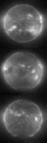
(a)

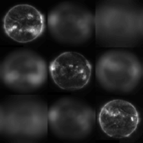
(b)

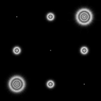
(c)

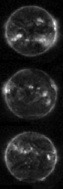
(d)

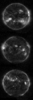
(e)

(f)

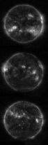
(g)

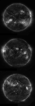
(h)

Figure 1: (a) Measured images for SNR = $20$ dB, (b) Contributions of each spectral component to the measurements, (c) Acting PSFs on spectral images, (d) Reconstructed images with TV, (e) Online patch-based dictionary, (f) Online convolutional dictionary, (g) Online convolutional dictionary with Tikhonov regularization and (h) Original Images.

Table 1: Parameters used for different priors.

Parameter	TV			PatchDic			ConvDic
SNR (dB)	$20$	$30$	$40$	$20$	$30$	$40$	$20$	$30$	$40$
$\lambda$	$10^{-2}$	$10^{-3}$	$10^{-4}$	$0.05$			$0.2$	$0.15$	$0.15$
$\beta$	$1$			$100$	$500$	$3000$	$2$	$8$	$50$
$\rho$	$10\lambda$			$1$			$50\lambda+0.5$
$\sigma$	$-$			$1$			$10$
$\mu$	$-$			$-$			$0.01$ (Tikhonov)

Table 2: Comparison of reconstruction PSNRs (dB) and SSIMs for different priors and SNRs.

		PatchDic	PatchDic	ConvDic	ConvDic	ConvDic	ConvDic
SNR (dB)	TV	KSVD	Online Update	Offline	Offline	Online Update	Online Update
					Tikhonov		Tikhonov
$20$	$32.62/{0.88}$	$32.45/0.86$	${32.97}/0.86$	$32.17/0.85$	$32.18/0.86$	$32.57/0.87$	$32.67/0.87$
$30$	$36.25/0.94$	$35.42/0.91$	$36.23/0.93$	$36.00/0.93$	$36.43/0.93$	$36.42/0.94$	${36.52/0.94}$
$40$	$39.57/0.97$	$38.42/0.95$	$39.21/0.96$	$39.21/0.96$	$39.63/0.97$	$39.80/0.97$	${39.83/0.97}$

For the photon sieve, a sample design [40] for EUV solar imaging is considered, with the smallest hole diameter of $5$ $\mu$m and the outer diameter of $25$ mm. Photon sieve is a diffractive lens whose focal length changes with the incoming wavelength. The PSSI system takes measurements at the focal planes of each of these three wavelengths, that is at $f_{1}$ = $3.754$ mm, $f_{2}$ = $3.742$ mm, and $f_{3}$ = $3.731$ mm. Then at the first focal plane, $f_{1}$, the measurement contains the focused image of the first spectral component at wavelength $\lambda_{1}=33.3$ nm, overlapped with the defocused spectral images of the remaining two components (at wavelengths $\lambda_{2}=33.4$ nm and $\lambda_{3}=33.5$ nm). Pixel size of the detector is chosen as $2.5\text{\,}\mathrm{\SIUnitSymbolMicro m}$ to match the diffraction-limited resolution of the imaging system.

The measurements are simulated using the forward model in Eq. (3) with white Gaussian noise. Here the number of measurements and the number of unknown spectral images are $K=S=3$. Fig. 1a shows the resulting measurements at the three focal planes with the contributions of each spectral component shown in Fig. 1b. These contributions are obtained by convolving the original spectral images in Fig. 1h, with the corresponding PSFs in Fig. 1b. The acting PSFs for the three spectral components are computed using the available PSF formula for the photon sieve [6, 41]. These PSFs illustrate the different amount of blur acting on spectral components. Hence the measurements involve not only the superposition of all spectral components but also significant amount of blur.

To analyze the performance with different noise levels, SNRs of $20$, $30$ and $40$ dB are considered. Reconstructions are obtained from the noisy measurements using Algorithm 1 and 2 with 2D priors. The parameters used for different priors are listed in Table 1. For the analysis case, we exploit 2D isotropic TV, which takes $20$ seconds for image reconstruction on a computer with 8 GB of RAM and i7 7500U 2.70 GHz CPU.

Secondly, we exploit a patch-based dictionary (PatchDic) with no online dictionary update. This dictionary is trained offline using the K-SVD algorithm [22] with $16$ representative solar images taken from the same database. We also use a randomly initialized patch-based dictionary, which is updated online throughout the iterations. For both cases, the number of patches extracted from each image is $N^{2}$ = $16384$ with one-stride. The patch size is numerically optimized as $6\times 6$, based on the simulations performed for $20$ dB SNR, which results in a dictionary size of $36\times 36$. Image reconstruction takes around $150$ and $200$ seconds with offline and online updated dictionary, respectively.

Moreover, we utilize convolutional dictionaries (ConvDic) in a similar manner. When an online dictionary update is not performed, the convolutional dictionary is trained offline with the same $16$ solar images. The dictionary size is numerically optimized as $12\times 12$ and the number of filters as $M=4$. Using this prior, a single reconstruction takes approximately $10$ and $20$ seconds with offline and online updated dictionary, respectively. The same experiments are also repeated by adding the gradient (Tikhonov) regularization, which result in similar reconstruction time.

Table 3: Comparison of reconstruction PSNRs (dB) / SSIMs / SAMs for different priors, datasets and SNRs.

Dataset	SNR (dB)	2D Wavelet $\operatorname*{\text{\raisebox{1.07639pt}{\scalebox{0.75}{$\bigotimes$}}}}$ 1D DCT	PatchDic	ConvDic	ConvDic (Tikhonov)
Objects	$20$	$24.82/11.78^{\circ}/0.82$	$25.42/11.13^{\circ}/0.77$	$26.71/10.16^{\circ}/0.77$	${26.82/9.64^{\circ}/0.84}$
	$30$	$26.18/10.57^{\circ}/0.88$	$26.78/10.03^{\circ}/0.85$	$28.42/8.64^{\circ}/0.85$	${28.54/8.49^{\circ}/0.89}$
	$40$	$27.76/9.30^{\circ}/0.89$	$28.91/8.35^{\circ}/0.87$	$29.63/7.71^{\circ}/0.89$	${30.15/7.44^{\circ}/0.91}$
Flowers	$20$	$27.94/20.06^{\circ}/0.77$	$28.82/21.61^{\circ}/0.80$	$28.16/21.26^{\circ}/0.78$	${28.31/19.76^{\circ}/0.79}$
	$30$	$31.09/{16.05^{\circ}}/0.87$	$31.57/17.68^{\circ}/0.88$	$30.47/18.64^{\circ}/0.85$	${31.19}/16.86^{\circ}/{0.88}$
	$40$	$33.46/15.04^{\circ}/0.92$	${35.16/13.26^{\circ}/0.93}$	$33.12/14.94^{\circ}/0.92$	${34.09/13.83^{\circ}/0.93}$
Pompoms	$20$	$28.02/{9.40^{\circ}}/0.83$	$28.66/10.27^{\circ}/0.82$	${28.54}/11.49^{\circ}/0.81$	$28.48/10.43^{\circ}/{0.83}$
	$30$	$29.29/{9.01^{\circ}}/0.87$	${30.44}/9.20^{\circ}/0.88$	$29.57/10.80^{\circ}/0.86$	${30.21}/9.41^{\circ}/{0.88}$
	$40$	$30.62/8.85^{\circ}/0.91$	${32.33}/8.15^{\circ}/{0.92}$	$30.40/10.13^{\circ}/0.90$	${31.41/8.71^{\circ}/0.92}$
Threads	$20$	$28.83/11.78^{\circ}/0.84$	$28.86/12.11^{\circ}/0.85$	$29.51/12.46^{\circ}/0.81$	$29.39/11.82^{\circ}/0.85$
	$30$	$31.14/10.79^{\circ}/0.90$	$32.52/10.44^{\circ}/0.90$	$31.82/11.79^{\circ}/0.87$	$32.27/10.29^{\circ}/0.90$
	$40$	$34.04/9.32^{\circ}/0.94$	$34.87/9.34^{\circ}/0.95$	$34.12/9.72^{\circ}/0.93$	$34.29/9.17^{\circ}/0.95$

The average reconstruction performance for all cases is given in Table 2 in terms of PSNR and SSIM. These average values are computed through $10$ Monte-Carlo runs for $4$ different spectral (solar) data sets. As seen from the table, PSNR is always above $32$ dB, and SSIM is above $0.85$, which demonstrate faithful reconstructions for all cases. Moreover, randomly initialized dictionary is effectively adapted to the data through online dictionary update, and yields higher PSNR and SSIM than the offline case for both patch-based and convolutional dictionaries.

To also visually evaluate the results, we provide sample reconstructions for SNR=$20$ dB case in Fig. 1d, 1e, 1f and 1g, together with the true images in Fig. 1h. Although TV prior, patch-based and convolutional dictionaries with online dictionary update provide similar reconstruction performance with comparable PSNR and SSIM values, visual comparison suggests that the image details are better preserved in the convolutional dictionary case. Moreover, convolutional dictionary and TV prior result in similar reconstruction times, whereas patch-based dictionary is approximately $10\times$ slower.

5.2 Case with correlations in three dimensions

The performance is now illustrated in PSSI system for a spectral data with 3D correlations. For this, we consider spectral datasets of size $256\times 256\times 16$ ($16$ wavelengths between $510-660$ nm with $10$ nm interval) taken from online spectral database referred as Objects [42], Flowers [43], Pompoms [43] and Threads [43]. For the photon sieve design, the smallest hole diameter is chosen as $15\text{\,}\mathrm{\SIUnitSymbolMicro m}$ and the outer diameter is $3.51$ mm. Moreover, the pixel size of the detector is chosen as $7.5\text{\,}\mathrm{\SIUnitSymbolMicro m}$  to match the diffraction-limited resolution of the imaging system. As before, the PSSI system takes measurements at the focal planes of each of these sixteen wavelengths. For example, for the wavelength at $580$ nm the focal length is $9.08$ cm. As a result, each measurement contains the focused image of one of the spectral components, overlapped with the defocused spectral images of the remaining fifteen components.

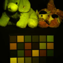
Figure 2: Datacube used for training.

The measurements are simulated again using the forward model in Eq. (3) with white Gaussian noise. Here the number of measurements and the number of unknown spectral images are $K=S=16$. To analyze the performance with different noise levels, SNRs of $20$, $30$ and $40$ dB are considered as before. Reconstructions are obtained from these noisy measurements using Algorithm 1 and 2 with 3D priors. The parameters used for different priors are listed in Table 4.

Table 4: Parameters used for different priors.

Parameter	Transform			PatchDic			ConvDic
SNR (dB)	$20$	$30$	$40$	$20$	$30$	$40$	$20$	$30$	$40$
$\lambda$	$0.5$	$0.1$	$0.01$	$0.0001$			$0.001$
$\beta$	$1$			$0.1$	$1$	$10$	$0.01$	$0.1$	$0.2$
$\rho$	$500\lambda$			$1000$			$1000$
$\sigma$	$-$			$10$			$10$
$\mu$	$-$			$-$			$0.1$ (Tikhonov)

Similar to the earlier spectral imaging approaches [3, 7], for the analysis case, we exploit a Kronecker basis as $\mathbf{T}$ = $\mathbf{T}_{1}\operatorname*{\text{\raisebox{1.07639pt}{\scalebox{0.75}{$\bigotimes$}}}}\mathbf{T}_{2}$ where $\mathbf{T}_{1}$ is the basis for 2D Symmlet-$8$ wavelet and $\mathbf{T}_{2}$ is the 1D discrete cosine (DCT) basis. This transformation is computed by first taking the wavelet transform of each spectral image and then 1D DCT along the spectral dimension. In this case, image reconstruction takes around 17 minutes.

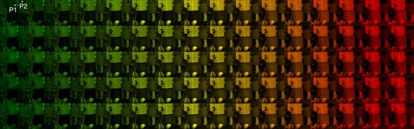
(a)

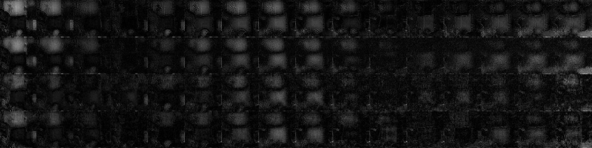
(b)

Figure 3: (a) Top-to-bottom: Original Images, reconstructed spectral images using 2D Symmlet $\operatorname*{\text{\raisebox{1.07639pt}{\scalebox{0.75}{$\bigotimes$}}}}$ 1D DCT transform, patch-based dictionary, convolutional dictionary and convolutional dictionary with Tikhonov regularization for SNR = $20$ dB, (b) The difference between original image and reconstructed images.

Secondly, we exploit a patch-based dictionary with online dictionary update. The initial dictionary is trained offline using the K-SVD algorithm with $25$ spectral datacubes of size $256\times 256\times 16$ cropped from Toys data [43] shown in Fig. 2. Here the patch size is chosen as $6\times 6\times 16$, resulting in a dictionary of size $576\times 576$. The number of patches extracted from each datacube is $N^{2}$ = $65536$ with one-stride only in spatial dimensions. In this case, image reconstruction takes around $100$ minutes.

Lastly, we utilize convolutional dictionaries. The initial convolutional dictionary is trained offline with the same $25$ spectral datacubes and then an online dictionary update is performed throughout the iterations. The dictionary size is numerically optimized as $32\times 32\times 5$ and the number of filters as $M=6$. Using this prior, a single reconstruction takes approximately $35$ minutes.

The average reconstruction performance for all cases is given in Table 3 in terms of PSNR, SSIM, and spectral angular mapper (SAM) [44]. These average values are computed through $10$ Monte-Carlo runs for each dataset. As seen from the table, the performance of different priors varies for different datasets and SNRs. In fact, each prior provides different capabilities over spatial and spectral dimensions.

To visually evaluate the results, we provide sample reconstructions in Fig. 3a for the Objects dataset and SNR = $20$ dB case, together with the true images. For easier interpretation and comparison of results, the absolute difference between the original spectral images and the reconstructed ones are shown in Fig. 3b as well. To investigate the recovery along the spectral dimension, we also select two representative points with different spectral characteristics, as shown as P1 and P2 in Fig. 3a. The reconstructed spectra of these points are plotted in Fig. 4a and 4b, together with the original spectra.

These results demonstrate that the chosen transform prior (2D Symmlet $\operatorname*{\text{\raisebox{1.07639pt}{\scalebox{0.75}{$\bigotimes$}}}}$ 1D DCT) generally yields smoother reconstructions over space and spectrum. Hence it can work fine if the original image data has smooth variations; however, this is generally not the case. As a result, this analysis prior often causes the largest errors due to the loss of image details along spatial and spectral directions, which can also be observed from higher SAM or lower PSNR/SSIM values.

On the other hand, with the patch-based dictionary, the spatial details are generally preserved better, but now there is additional unwanted grainy structure in space. Nevertheless, it often achieves the highest PSNR and SSIM. However, same is not true for the spectral recovery. The spectra recovered with the patch-based dictionary are generally overly smooth, resulting in the worst reconstruction performance along the spectral dimension and the highest SAM values. One possible cause here is the chosen patch size, which does not perform partitioning in the spectral dimension. But note that the reconstruction with this patch size is already $3\times$ slower than the convolutional dictionary and $6\times$ slower than the transform-based alternative. Hence working with smaller patches along spectrum will bring much higher computational cost.

The results suggest that convolutional dictionary provides a better trade-off between reconstruction performance and time compared to the patch-based one. With the convolutional prior, the resulting errors are more uniform over space and spectrum. That is, both spatial and spectral characteristics (variations) are generally well-preserved in the reconstructions, as can also be seen from high PSNR/SSIM and low SAM values. As expected, the inclusion of Tikhonov regularization yields a smoother reconstruction and less grainy spatial structure, but may come with the slight cost of loss of some spatial details.

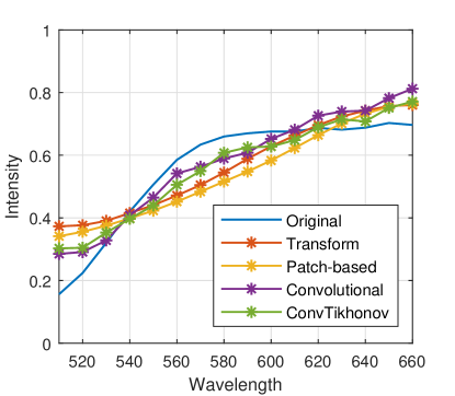
(a)

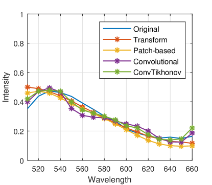
(b)

Figure 4: (a) Spectra at the points P1, and (b) P2 for SNR = $20$ dB.

6 Conclusion

In this paper, we have developed a unified framework for the solution of a general class of inverse problems, namely convolutional inverse problems, that are widely encountered in multidimensional imaging. Considering a general image-formation model and using ADMM, we developed fast image reconstruction algorithms that can exploit different analysis and synthesis priors as well as correlations in different dimensions. In the analysis case, multidimensional sparsifying operators are utilized. In the synthesis case, convolutional or patch-based dictionaries are exploited and adapted to correlations in different dimensions.

To illustrate their utility and versatility, the developed algorithms with different priors are applied to 3D reconstruction problems in computational spectral imaging, and their performance is comparatively evaluated for various cases with and without correlation along the third dimension. Although analysis priors performed best in terms of reconstruction time, image details were generally better preserved with dictionary-based priors. The results suggest that convolutional dictionary provides a better trade-off between reconstruction performance and time. Future work can focus on exploiting other structured dictionaries such as those with tensor or Kronecker structure [45, 46, 47, 48].

The versatile ADMM-based reconstruction algorithms developed in this paper are broadly applicable to linear shift-variant imaging systems whose response slowly varies across the field of view, time, depth, or spectral dimensions. Moreover, the algorithms can be parallelized and easily extended to use with other priors such as those based on deep learning. As the advent of multidimensional imaging modalities expands to perform sophisticated tasks, these algorithms are essential for fast iterative reconstruction in various large-scale problems.

References

- [1] Liang Gao and Lihong V. Wang. A review of snapshot multidimensional optical imaging: Measuring photon tags in parallel. Physics Reports, 616:1–37, 2016.
- [2] Figen S Oktem, Liang Gao, and Farzad Kamalabadi. Computational spectral and ultrafast imaging via convex optimization. In Handbook of Convex Optimization Methods in Imaging Science, pages 105–127. Springer, 2018.
- [3] R. M. Willett, M. F. Duarte, M. A. Davenport, and R. G. Baraniuk. Sparsity and structure in hyperspectral imaging: Sensing, reconstruction, and target detection. IEEE Signal Processing Magazine, 31(1):116–126, 2014.
- [4] Jo Schlemper, Jose Caballero, Joseph V. Hajnal, Anthony N. Price, and Daniel Rueckert. A deep cascade of convolutional neural networks for dynamic MR image reconstruction. IEEE Transactions on Medical Imaging, 37(2):491–503, 2018.
- [5] Nick Antipa, Grace Kuo, Reinhard Heckel, Ben Mildenhall, Emrah Bostan, Ren Ng, and Laura Waller. DiffuserCam: lensless single-exposure 3D imaging. Optica, 5(1):1–9, 2018.
- [6] Figen S Oktem, Farzad Kamalabadi, and Joseph M Davila. High-resolution computational spectral imaging with photon sieves. In 2014 IEEE International Conference on Image Processing (ICIP), pages 5122–5126. IEEE, 2014.
- [7] Oguzhan Fatih Kar and Figen S. Oktem. Compressive spectral imaging with diffractive lenses. Optics Letters, 44(18):4582–4585, 2019.
- [8] Loic Denis, Eric Thiebaut, Ferreol Soulez, Becker Jean-Marie, and Rahul Mourya. Fast approximations of shift-variant blur. International Journal of Computer Vision, 115:253–278, 2015.
- [9] Filip Sroubek, Jan Kamenicky, and Yue Lu. Decomposition of space-variant blur in image deconvolution. IEEE Signal Processing Letters, 23:346–350, 2016.
- [10] Didem Dogan and Figen S Oktem. Convolutional inverse problems in imaging with convolutional sparse models. In Imaging and Applied Optics 2019 (COSI, IS, MATH, pcAOP), pages JW2A–9. Optical Society of America, 2019.
- [11] Andrea La Camera, Laura Schreiber, Emiliano Diolaiti, Patrizia Boccacci, M. Bertero, Michele Bellazzini, and Paolo Ciliegi. A method for space-variant deblurring with application to adaptive optics imaging in astronomy. Astronomy & Astrophysics, 579, 2015.
- [12] Xin Zhang and Edmund Lam. Edge-preserving sectional image reconstruction in optical scanning holography. JOSA A, 27:1630–1637, 2010.
- [13] Daniel Badali and R. Miller. Robust reconstruction of time-resolved diffraction from ultrafast streak cameras. Structural Dynamics, 4:054302, 2017.
- [14] Urvashi Rau and Tim J Cornwell. A multi-scale multi-frequency deconvolution algorithm for synthesis imaging in radio interferometry. Astronomy & Astrophysics, 532:A71, 2011.
- [15] IM Stewart, DM Fenech, and TWB Muxlow. A multiple-beam clean for imaging intra-day variable radio sources. Astronomy & Astrophysics, 535:A81, 2011.
- [16] Min-Oh Kim, Sang-Young Zho, and Donghyun Kim. 3D imaging using magnetic resonance tomosynthesis (MRT) technique. Medical Physics, 39(8):4733–4741, 2012.
- [17] Derya Gol Gungor and Lee C Potter. A subspace-based coil combination method for phased-array magnetic resonance imaging. Magnetic Resonance in Medicine, 75(2):762–774, 2016.
- [18] Mihai Florea, Adrian Basarab, Denis Kouamé, and Sergiy Vorobyov. An axially-variant kernel imaging model for ultrasound image reconstruction. IEEE Signal Processing Letters, 5(3):381–394, 2018.
- [19] Adrien Besson, Lucien Roquette, Dimitris Perdios, Matthieu Simeoni, Marcel Arditi, Paul Hurley, Yves Wiaux, and Jean-Philippe Thiran. A physical model of non-stationary blur in ultrasound imaging. IEEE Transactions on Computational Imaging, 25(7):961–965, 2019.
- [20] Stephen Boyd, Neal Parikh, Eric Chu, Borja Peleato, and Jonathan Eckstein. Distributed optimization and statistical learning via the alternating direction method of multipliers. Found. Trends Mach. Learn., 3(1):1––122, 2011.
- [21] Michael Elad, Peyman Milanfar, and Ron Rubinstein. Analysis versus synthesis in signal priors. Inverse Problems, 23:947, 2007.
- [22] M. Aharon, M. Elad, and A. Bruckstein. K - SVD: An algorithm for designing overcomplete dictionaries for sparse representation. IEEE Trans. Sig. Proc., 54(11):4311–4322, 2006.
- [23] Saiprasad Ravishankar and Yoram Bresler. MR image reconstruction from highly undersampled k-space data by dictionary learning. IEEE Transactions on Medical Imaging, 30(5):1028–1041, 2010.
- [24] Jose Caballero, Anthony N Price, Daniel Rueckert, and Joseph V Hajnal. Dictionary learning and time sparsity for dynamic MR data reconstruction. IEEE Transactions on Medical Imaging, 33(4):979–994, 2014.
- [25] Oana Lorintiu, Hervé Liebgott, Martino Alessandrini, Olivier Bernard, and Denis Friboulet. Compressed sensing reconstruction of 3D ultrasound data using dictionary learning and line-wise subsampling. IEEE Transactions on Medical Imaging, 34:2467–2477, 2014.
- [26] Brendt Wohlberg. Efficient algorithms for convolutional sparse representations. IEEE Transactions on Image Processing, 25(1):301–315, 2016.
- [27] Xuemei Hu, Felix Heide, Qionghai Dai, and Gordon Wetzstein. Convolutional sparse coding for RGB+ NIR imaging. IEEE Transactions on Image Processing, 27(4):1611–1625, 2017.
- [28] Cristina Garcia-Cardona and Brendt Wohlberg. Convolutional dictionary learning: A comparative review and new algorithms. IEEE Transactions on Computational Imaging, 4(3):366–381, 2018.
- [29] Thanh Nguyen-Duc, Tran Minh Quan, and Won-Ki Jeong. Frequency-splitting dynamic mri reconstruction using multi-scale 3D convolutional sparse coding and automatic parameter selection. Medical image analysis, 53:179–196, 2019.
- [30] Crisostomo Barajas-Solano, Juan-Marcos Ramirez, and Henry Arguello. Convolutional sparse coding framework for compressive spectral imaging. Journal of Visual Communication and Image Representation, 66:102690, 2020.
- [31] Ives Rey-Otero, Jeremias Sulam, and Michael Elad. Variations on the convolutional sparse coding model. IEEE Transactions on Signal Processing, 68:519–528, 2020.
- [32] Yifei Lou, Tieyong Zeng, Stanley J. Osher, and Jack Xin. A weighted difference of anisotropic and isotropic total variation model for image processing. SIAM J. Imaging Sciences, 8(3):1798–1823, 2015.
- [33] Singanallur V. Venkatakrishnan and Brendt Wohlberg. Convolutional dictionary regularizers for tomographic inversion. In Proceedings of IEEE International Conference on Acoustics, Speech, and Signal Processing (ICASSP), pages 7820–7824, Brighton, UK, 2019.
- [34] Brendt Wohlberg. Convolutional sparse representations as an image model for impulse noise restoration. In Proceedings of the IEEE Image, Video, and Multidimensional Signal Processing Workshop (IVMSP), pages 1–5, Bordeaux, France, 2016.
- [35] M. Afonso, J. Bioucas-Dias, and M. A. T. Figueiredo. Fast image recovery using variable splitting and constrained optimization. IEEE Transactions on Image Processing, 19(9):2345–2356, 2010.
- [36] Ulas Kamaci, Fatih C Akyon, Tunc Alkanat, and Figen S Oktem. Efficient sparsity-based inversion for photon-sieve spectral imagers with transform learning. In 2017 IEEE Global Conference on Signal and Information Processing (GlobalSIP), pages 1225–1229. IEEE, 2017.
- [37] Ben Noble and James W Daniel. Applied linear algebra, volume 3. Prentice-Hall New Jersey, 1988.
- [38] Antonin Chambolle. An algorithm for total variation minimization and applications. Journal of Mathematical Imaging and Vision, 20(1-2):89–97, 2004.
- [39] K. Addison. SDO — Solar Dynamics Observatory, 2020. Accessed = 2019-11-01.
- [40] Joseph M Davila. High-resolution solar imaging with a photon sieve. In Solar Physics and Space Weather Instrumentation IV, volume 8148, page 81480O. International Society for Optics and Photonics, 2011.
- [41] Figen S. Oktem, Farzad Kamalabadi, and Joseph M. Davila. Analytical Fresnel imaging models for photon sieves. Opt. Express, 26(24):32259–32279, Nov 2018.
- [42] Sérgio M. C. Nascimento, Flávio P. Ferreira, and David H. Foster. Statistics of spatial cone-excitation ratios in natural scenes. J. Opt. Soc. Am. A, 19(8):1484–1490, 2002.
- [43] Fumihito Yasuma, Tomoo Mitsunaga, Daisuke Iso, and Shree K Nayar. Generalized assorted pixel camera: postcapture control of resolution, dynamic range, and spectrum. IEEE Transactions on Image Processing, 19(9):2241–2253, 2010.
- [44] B. Park, William Windham, K.C. Lawrence, and D.P. Smith. Contaminant classification of poultry hyperspectral imagery using a spectral angle mapper algorithm. Biosystems Engineering, 96:323–333, 2007.
- [45] Cesar F Caiafa and Andrzej Cichocki. Computing sparse representations of multidimensional signals using Kronecker bases. Neural computation, 25(1):186–220, 2013.
- [46] Oguz Semerci, Ning Hao, Misha E Kilmer, and Eric L Miller. Tensor-based formulation and nuclear norm regularization for multienergy computed tomography. IEEE Transactions on Image Processing, 23(4):1678–1693, 2014.
- [47] Sara Soltani, Misha E Kilmer, and Per Christian Hansen. A tensor-based dictionary learning approach to tomographic image reconstruction. BIT Numerical Mathematics, 56(4):1425–1454, 2016.
- [48] Qi Xie, Qian Zhao, Deyu Meng, and Zongben Xu. Kronecker-basis-representation based tensor sparsity and its applications to tensor recovery. IEEE Transactions on Pattern Analysis and Machine Intelligence, 40(8):1888–1902, 2018.