11institutetext: 🖂 Xin Xu
11email: xu.permanent@gmail.com 22institutetext: Department of Control and Systems Engineering, School of Management and Engineering, Nanjing University, Nanjing, 210008, China
Department of Chemistry, Princeton University, Princeton, NJ 08544, USA
33institutetext: Xiaopeng Luo
33email: luo.permanent@gmail.com 44institutetext: Department of Control and Systems Engineering, School of Management and Engineering, Nanjing University, Nanjing, 210008, China
Department of Chemistry, Princeton University, Princeton, NJ 08544, USA
55institutetext: Daoyi Dong
55email: daoyidong@gmail.com 66institutetext: School of Engineering and Information Technology, University of New South Wales, Canberra, 2600, Australia
Derivative-free global minimization for a class of multiple minima problems
Xiaopeng Luo
Xin Xu
Daoyi Dong
Abstract
We prove that the finite-difference based derivative-free descent (FD-DFD) methods have a capability to find the global minima for a class of multiple minima problems. Our main result shows that, for a class of multiple minima objectives that is extended from strongly convex functions with Lipschitz-continuous gradients, the iterates of FD-DFD converge to the global minimizer with the linear convergence for a fixed and any initial iteration when the parameters are properly selected. Since the per-iteration cost, i.e., the number of function evaluations, is fixed and almost independent of the dimension , the FD-DFD algorithm has a complexity bound for finding a point such that the optimality gap is less than . Numerical experiments in various dimensions from to demonstrate the benefits of the FD-DFD method.
Keywords:
multiple minima problem global minima nonconvex derivative-free convergence rate complexity
The FD-DFD method could be regarded as a smoothed extension of the gradient method because an FD-DFD descent direction is an unbiased estimate of smoothed gradient at the current iterate NemirovskiA1983M_optimization ; NesterovY2017A_GF . It also has some characteristics of the gradient method NesterovY2017A_GF but its “cognitive range” is closely related to the smoothing parameter. One may expect that the FD-DFD method has certain global search capability when the smoothing and stepsize parameters are properly selected. Therefore, we attempt to analyze the convergence behavior of the FD-DFD method in global optimization under certain conditions, regardless of whether the derivative is available.
Recently, a regularized asymptotic descent (RAD) method LuoX2020A_RAD was proposed to find the global minima with linear convergence and logarithmic work complexity for certain class of multiple minima problems. It is inspired by an asymptotic solution of the regularized minimization problems which is extended from the Pincus asymptotic solution formula PincusM1968A_AsymptoticSolution ; PincusM1970A_AsymptoticSolution . Under a mild assumption, the RAD iterates will converge to the global minimizer without being trapped in saddle points, local minima, or even discontinuities. In this work, we will prove that the FD-DFD method also enjoys a similar convergence behavior under the same assumption.
Specifically, we analyze the FD-DFD method for finding the global minima
(1)
where the objective function satisfies the following assumption:
Assumption 1
The objective function satisfies there exist and such that for all ,
(2)
Hence, has a unique global minimizer with .
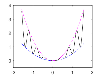
Figure 1: One-dimensional examples. Left: the objective (solid) with lower bound (dashed) and upper bound (dash-dotted). Right: the objective (solid) with lower bound (dashed) and upper bound (dash-dotted).
As shown in Fig. 1, such a class of functions can be extended from strongly convex functions with Lipschitz-continuous gradients; however, it is not ruling out the possibility of multiple minima. The lower bound guarantees the uniqueness of the global minima while the upper bound controls the sharpness of the minima.
Under Assumption 1, the Lipschitz-continuous objective has a unique global minima and possibly multiple local minima. Our goal here is to find this global minima without being trapped in saddle points or local minima. We prove that the FD-DFD method enjoys global linear convergence, i.e., , for finding the global minimizer when the parameters are properly selected (see Theorem 2.3).
The remainder of the paper is organized as follows. In Sect. 2, we establish the convergence property and complexity bound
for the FD-DFD method. In Sect. 3, we compare the characteristics of the FD-DFD method with the RAD method. In Sect. 4, we demonstrate the benefits of the FD-DFD method by numerical experiments in various dimensions from to . And finally, we draw conclusions in Sect. 5.
2 Derivative-free methods
2.1 Gradient of Gaussian smoothing
Let random vector have -dimensional standard normal distribution, that is, . Denote by the expectation of corresponding random variable. For any smoothing parameter , we consider
as an unbiased estimate for the gradient of the smoothed objective function
(3)
In practice, and can be replaced with corresponding estimate.
Using the substitution , this gradient estimate can also be written as
Theorem 2.1 establishes , thus, we obtain the unbiasedness
Theorem 2.1
Suppose that is the smoothed objective with a smoothing parameter defined by (3), then its gradient
(4)
where and .
Proof
Using the substitution , we obtain
and therefore,
That is, . Using the substitution , we further obtain
and the proof is complete. ∎
We will see that the smoothed gradient plays a key role in the subsequent analysis. At the same time, we also notice that the Gaussian smoothing does not make any significant changes to the bounds of the objective function . Specifically, under Assumption 1, we have,
together with
we obtain the bounds
2.2 Algorithms
With an initial point , a stepsize , an initial exploration radius , a fixed contraction factor and a number of function evaluations per-iteration , the FD-DFD method is characterized by the iteration
(5)
where the gradient estimate
(6)
here, and . To increase the stability of the iteration, we recommend to use the gradient estimate
(7)
where
Here the random vector has -dimensional standard normal distribution.
Note that, if as , can be viewed as an estimate for
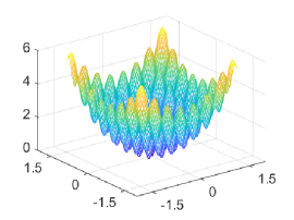
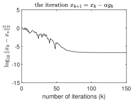
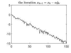
we can obtain ; and futher, . The difference between these two iterations based on and is shown in Fig. 2. We can see that when the stepsize parameter is properly selected, they have almost the same convergence behavior in the early stage while the estimate is more stable than the estimate as the iteration progresses. Hence, we mainly consider the gradient estimate in the following. Now we present the FD-DFD method as Algorithm 1.
Figure 2: Difference between two iterations. Left: the objective . Middle: the iteration with parameter settings , , , and . Right: the iteration with parameter settings , , , and .Algorithm 1 FD-DFD Method
1: Choose an initial iterate and preset parameters , , , .
2:fordo
3: Set the variance .
4: Generate realizations of from .
5: Compute a stochastic vector .
6: Set the new iterate as .
7:endfor
It follows from Chebyshev’s inequality and that, for all and any , with probability at least , the -th component of satisfies
(8)
Furthermore, the -th component of satisfies
(9)
2.3 Analyses
To establish the expected linear convergence of the FD-DFD method, we first build upper bounds for and by the following two lemmas.
Lemma 2.1
Under Assumption 1, suppose that with and there is an such that . Then for any , the -th component of satisfies the following inequality:
further, when , this inequality can be improved as
then for any , together with the definition of , we further obtain
Since
it follows that
and the proof is complete.∎
Theorem 2.2
Under Assumption 1, suppose that with and there is an such that for all . If the FD-DFD method (Algorithm 1) is run with a stepsize parameter such that
then with probability at least , the iterates of FD-DFD satisfy:
where the constant
is independent of but depends on .
Proof
According to (8), Lemmas 2.1 and 2.2, it holds that for any and all , with probability at least ,
further, by the Arithmetic Mean Geometric Mean inequality, we have
Finally, by summing from to , one obtains
and doing it recursively, one further obtains,
and the proof is complete.∎
The following theorem states that when the parameters are properly selected, the iterates of FD-DFD satisfy for all in probability.
Theorem 2.3
Under Assumption 1, suppose that with . If the FD-DFD method (Algorithm 1) is run with a stepsize parameter such that
then with high probability, the iterates of FD-DFD satisfy for all :
where and
Proof
Let , that is, , which satisfies the condition of Theorem 2.2. Using Theorem 2.2 and induction, one can deduce
Notice that for every , it follows that
thus, one can finally obtain
and the proof is complete.∎
Since is independent of , the following total work complexity bound for the FD-DFD method is immediate from Theorem 2.3.
Corollary 2.1 (Complexity bound)
Suppose the conditions of Theorem 2.3 hold. Then the
number of function evaluations of the FD-DFD (Algorithm 1) required to achieve is .
3 Comparison of RAD and FD-DFD
With an initial point , three fixed parameters , and , the RAD method LuoX2020A_RAD is characterized by the iteration
(10)
With an additional stepsize parameter , the FD-DFD method is characterized by the iteration
(11)
where and . In practice, and should be replaced with corresponding estimates.
Both the RAD and FD-DFD method have their own characteristics. Since RAD is based on the asymptotic representation for the solution of regularized minimization, it does not require a stepsize parameter, or in other words, it can automatically obtain the optimal stepsize; however, the parameter in RAD algorithms increases as the dimension increases (See Fig. 3 in LuoX2020A_RAD ). In comparison, the parameter in FD-DFD algorithms is almost independent of because the variance term containing is insignificance for an appropriate (See Fig. 3 and Theorem 2.2); but as a price, there is an additional stepsize parameter and the choice of directly affects whether the iterate sequence will converge to the global minimizer.
4 Numerical experiments
We illustrate the performance of the FD-DFD algorithm by considering the revised Rastrigin function in defined as
As shown in Fig. 1, this revised Rastrigin function satisfies Assumption 1. It has a unique global minima located at the origin and many local minima, e.g., the number of its local minima reaches in the hypercube .
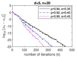
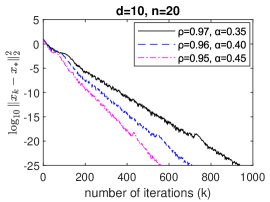
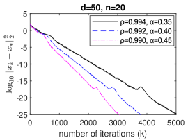
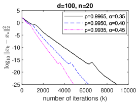
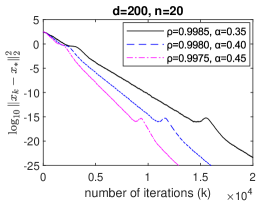
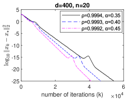
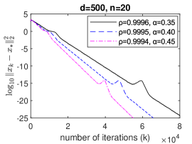
Fig. 3 shows the performance of FD-DFD algorithms for the revised Rastrigin function in various dimensions from to . These experiments clearly demonstrate the global linear convergence of the FD-DFD method.
Figure 3: Performance of the FD-DFD method for the revised Rastrigin function in various dimensions, every initial iterate is randomly selected on a sphere of radius centered at the origin, the parameter , three different settings for the parameters and are run independently for each plot.
In these experiments, every initial iterate is randomly selected on a -dimensional sphere of radius centered at the origin. Furthermore, the random vectors in each iteration are sequentially generated by a halton sequence with RR scramble type KocisL1997A_QMCscramble . The algorithm is implemented in Matlab. The source code of the implementation is available at https://github.com/xiaopengluo/dfd.
5 Conclusions
In this work we have analyzed that the finite-difference derivative-free descent (FD-DFD) method enjoys linear convergence for finding the global minima of a class of multiple minima functions. It also has a total work complexity bound to find a point such that the gap between this point and the global minimizer is less than . Numerical experiments in various dimensions demonstrate all the benefits.
Acknowledgements.
We thank Prof. Herschel A. Rabitz for several discussions about global optimization for multiple minima problems.
References
(1)
Bergstra, J., Bengio, Y.: Random search for hyper-parameter optimization.
Journal of Machine Learning Research 13, 281–305 (2012)
(2)
Burke, J.V., Chen, X., Sun, H.: The subdifferential of measurable composite max
integrands and smoothing approximation.
Mathematical Programming 181, 229–264 (2020)
(4)
Conn, A., Scheinberg, K., Vicente, L.: Introduction to derivative-free
optimization.
MPS-SIAM series on optimization, SIAM, Philadelphia (2009)
(5)
Duchi, J.C., Bartlett, P.L., Wainwright, M.J.: Randomized smoothing for
stochastic optimization.
SIAM J. Optim. 22(2), 674–701 (2012)
(6)
Duchi, J.C., Jordan, M.I., Wainwright, M.J., Wibisono, A.: Optimal rates for
zero-order convex optimization: The power of two function evaluations.
IEEE Trans. Information Theory 61(5), 2788–2806 (2015)
(7)
Hazan, E.E., Levy, K.Y.: Bandit convex optimization: Towards tight bounds.
Advances in Neural Information Processing Systems 1,
784–792 (2014)
(8)
Jin, C., Ge, R., Netrapalli, P., Kakade, S.M., Jordan, M.I.: How to escape
saddle points efficiently.
In: Proceedings of the 34th International Conference on Machine
Learning (PMLR), vol. 70, pp. 1724–1732 (2017)
(9)
Kocis, L., Whiten, W.J.: Computational investigations of low-discrepancy
sequences.
ACM Transactions on Mathematical Software 23(2), 266–294
(1997)
(10)
Luo, X., Xu, X.: Regularized asymptotic descents: finding the global minima for
a class of multiple minima problems (2020).
ArXiv:2004.02210
(11)
Nemirovski, A., Yudin, D.: Problem complexity and method efficiency in
optimization.
John Wiley and Sons, New York (1983)
(13)
Nesterov, Y., Spokoiny, V.: Random gradient-free minimization of convex
functions.
Found. Comput. Math. 17(2), 527–566 (2017)
(14)
Pemantle, R.: Nonconvergence to unstable points in urn models and stochastic
approximations.
The Annals of Probability 18(2), 698–712 (1990)
(15)
Pincus, M.: A closed form solution of certain programming problems.
Operations Research 16(3), 690–694 (1968)
(16)
Pincus, M.: A monte carlo method for the approximate solution of certain types
of constrained optimization problems.
Operations Research 18(6), 1225–1228 (1970)
(17)
Poliak, B.T.: Introduction to optimization.
Optimization Software, Inc., New York (1987)
(18)
Shamir, O.: An optimal algorithm for bandit and zero-order convex optimization
with two-point feedback.
Journal of Machine Learning Research 18, 1–11 (2017)