A Generalization of Bellman’s Equation with Application to Path Planning, Obstacle Avoidance and Invariant Set Estimation

Abstract

The standard Dynamic Programming (DP) formulation can be used to solve Multi-Stage Optimization Problems (MSOP’s) with additively separable objective functions. In this paper we consider a larger class of MSOP’s with monotonically backward separable objective functions; additively separable functions being a special case of monotonically backward separable functions. We propose a necessary and sufficient condition, utilizing a generalization of Bellman’s equation, for a solution of a MSOP, with a monotonically backward separable cost function, to be optimal. Moreover, we show that this proposed condition can be used to efficiently compute optimal solutions for two important MSOP’s; the optimal path for Dubin’s car with obstacle avoidance, and the maximal invariant set for discrete time systems.

, ,

1 Introduction

Throughout Engineering, Economics, and Mathematics many problems can be formulated as Multi-Stage Optimization Problems (MSOP’s):

$$\min \bigg{\{}J(u(0),...,u(T-1),x(0),...,x(T))\bigg{\}}$$

$$x(0)=x_{0},\text{ }x(t+1)=f(x(t),u(t),t)\text{ for }t={0},..,T-1$$

$$x(t)\in X_{t}\subset\mathbb{R}^{n},\text{ }u(t)\in U\subset\mathbb{R}^{m}\text{ for }t={0},..,T.$$

Such problems consist of 1) a cost function $J:\mathbb{R}^{m\times T}\times\mathbb{R}^{n\times(T+1)}\to\mathbb{R}$, 2) an underlying discrete-time dynamical system governed by the plant equation $f:\mathbb{R}^{n}\times\mathbb{R}^{m}\times\mathbb{N}\to\mathbb{R}^{n}$, 3) a state space $X_{t}\subset\mathbb{R}^{n}$, 4) an admissible input space $U\subset\mathbb{R}^{m}$, and 5) a terminal time $T>0$. Examples of such optimization problems include: optimal battery scheduling to minimize consumer electricity bills [11]; energy-optimal speed planning for road vehicles [33]; optimal maintenance of manufacturing systems [21]; etc.

MSOP’s are members of the class of constrained nonlinear optimization problems. Such optimization problems can be solved using nonlinear solvers such as SNOPT [8] over small time horizons. However, the most commonly used class of methods for solving MSOP’s is Dynamic Programming (DP) [2]. DP methods exploit the structure of MSOP’s to decompose the optimization problem into lower dimensional sub-problems that can be solved recursively to give the solution to the original higher dimensional MSOP. Typically, DP is used to solve problems with cost functions of the form $J(\mathbf{u},\mathbf{x})=\sum_{t=0}^{T-1}c_{t}(x(t),u(t))+c_{T}(x(T))$. These functions (Defn. 2) are called additively separable functions, as they can be additively separated into sub-functions, each of which only depend on a single time-stage, $t\in\{0,...,T\}$. In the additively separable case it was shown in [1] that if we can find a function $F$ that satisfies Bellman’s Equation,

$$F(x,T) =c_{T}(x)\quad\text{for all }x\in X_{T}$$

$$F(x,t) =\inf_{u\in\Gamma_{x,t}}\bigg{\{}c_{t}(x,u)+F(f(x,u,t),t+1)\bigg{\}}$$

$$\qquad\qquad\qquad\text{for all }x\in X_{t},t\in\{0,..,T-1\},$$

where $\Gamma_{x,t}:=\{u\in U:f(x,u,t)\in X_{t}\}$, then a necessary and sufficient condition for a feasible input and state sequence, $\mathbf{u}=(u(0),...,u(T-1))$ and $\mathbf{x}=(x(0),...,x(T))$, to be optimal is

$$u(t)\in\arg\inf_{u\in\Gamma_{x(t),t}}\bigg{\{}c_{t}(x(t),u) +F(f(x(t),u,t),t+1)\bigg{\}}$$

$$\text{for all }t\in\{0,..,T-1\}.$$

We consider MSOP’s with cost functions of the more general form $J(\mathbf{u},\mathbf{x})=\phi_{0}(x(0),u(0),\phi_{1}(x(1),u(1),\dots\phi_{T}(x(T))\dots))$, where maps $\phi_{t}:X_{t}\times U\times\mathbb{R}\to\mathbb{R}$ are monotonic in their third argument for $t=0,\cdots T-1$. Such functions are called monotonically backward separable, defined in Definition 3, and shown to contain the class of additively separable functions in Lemma 4. For MSOP’s with monotonically backward separable cost functions we show in Theorem 10 that if we can find a function $V$ that satisfies

$$V(x,T) =\phi_{T}(x)\quad\text{for all }x\in X_{T}$$ (1)

$$V(x,t) =\inf_{u\in\Gamma_{x,t}}\bigg{\{}\phi_{t}(x,u,V(f(x,u,t),t+1))\bigg{\}}$$

$$\qquad\qquad\qquad\qquad\text{for all }x\in X_{t},t\in\{0,..,T-1\},$$

where $\Gamma_{x,t}:=\{u\in U:f(x,u,t)\in X_{t}\}$, then a necessary and sufficient for a feasible input and state sequence, $\mathbf{u}=(u(0),...,u(T-1))$ and $\mathbf{x}=(x(0),...,x(T))$, to be optimal is

$$u(t)\in\arg\inf_{u\in\Gamma_{x(t),t}}\bigg{\{}\phi_{t}\left(x(t),u,V(f(x(t),u,t),t+1)\right)\bigg{\}}$$

$$\hskip 128.0374pt\text{for all }t\in\{0,..,T-1\}.$$

Equation (1) can be thought of as a generalization of Bellman’s Equation; as it is shown in Corollary 11 that in the special case when the cost function is additively separable Equation (1) reduces to Bellman’s Equation. We therefore refer to Equation (1) as the Generalized Bellman’s Equation (GBE). Through several examples we show a solution, $V$, to the GBE can be obtained numerically by recursively solving the GBE backwards in time for each element of $X_{t}$, the same way Bellman’s Equation is solved, thereby extending traditional DP methods to solve a larger class of MSOP’s with non-additively separable cost functions. Moreover, in Section 4 it is shown how Approximate Dynamic Programming (ADP) methods can be modified to solve the GBE.

By recursively solving the GBE (1) it is possible to synthesize optimal input sequences for many important practical problems. In this paper we consider two such problems; path planning with obstacle avoidance and maximal invariant sets. First, we define the path planning problem as the search for a sequence of inputs that drives a dynamical system to a target set in minimum time while avoiding obstacles defined by subsets of the state-space. In Section 5 we show that such problems can be formulated as an MSOP with monotonically backward separable objective, of form $J(\mathbf{u},\mathbf{x})=\min\left\{\inf\left\{t\in[0,T]:x(t)\in S\right\},T\right\}$, implying that the solution to the path planning problem can be found using the solution to the GBE. Similarly, in Section 6 we show that computation of maximal invariant sets can be formulated as an MSOP with monotonically backward separable objective of form $J(\mathbf{u},\mathbf{x})=\max\{\max_{0\leq k\leq T-1}\{c_{k}(u(k),x(k))\},c_{T}(x(T))\}$.

Path planning with obstacle avoidance has been extensively studied (see surveys [5] [7]) and has many applications; including UAV surveillance [31]. In [25] the path planning problem is separated into two separate problems: the “geometric problem”, in which the shortest curve, $\tilde{x}(t)$, between the initial set and target set is calculated, and the “tracking problem”, in which a controller, $u(t)$, is synthesized so that $\sum_{t=0}^{T}||x(t)-\tilde{x}(t)||_{2}^{2}$ is minimized, where $x(t+1)=f(x(t),u(t),t)$ and $||\cdot||_{2}$ is the Euclidean norm. Separating the path planning problem allows for the use of efficient algorithms such as $A^{*}$-search or tangent graphs [22] to solve the “geometric problem” and LQR control to solve the “tracking problem”, however, there is no guaranteed that this method will produce the true solution to the original path planning problem. The same approach is used in [4], where it is shown through numerical examples that a controller closer to optimality can be derived when the state space is augmented with historic trajectory information. Our approach of using the GBE to solve the path planning does not separate the problem into the “geometric or “tracking” problem and thus does not require any state augmentation. For systems described in continuous time (rather than the discrete systems considered in this paper) with obstacles that satisfy certain boundary curvature assumptions, assumptions not made in this paper, it has been shown in [27] that a path planning sliding mode controller can be efficiently computed. Furthermore, this sliding mode controller can be used for effective path planning in unknown environments, a case not considered in this paper.

The GBE can also be used in the application of computing the Finite Time Horizon Maximal Invariant Set (FTHMIS), defined as the largest set of initial conditions for a discrete time process such that there exists a feasible input sequence for which the state of the system never violates a time-varying constraint. Knowledge of this set can be used to design controllers that ensure the system never violates given safety constraints. We show that FTHMIS’s are equivalent to the sublevel set of solutions to the GBE. To the best of the authors knowledge the problem of computing FTHMIS’s has not previously been addressed in the literature. However, a proposed methodology for computing maximal invariant sets over infinite time horizons can be found in [32, 6, 30]. Similar continuous-time formulations of this problem can be found in [15, 14].

Substantial work on generalizations of Bellman’s Equation for both infinite and finite time MSOP’s can be found in [3]. Our work differs from [3] as rather than attempting to generalize the ”Bellman’s operator“, as [3] does, we consider a wider class of cost functions associated with MSOP’s, introducing monotonically backward separable cost functions, leading to a derivation of the GBE (1). Unlike in [3], we formalize the link between the cost function of an MSOP and the GBE (1). Other examples in the literature of MSOP’s with non-additively separable cost functions can be found in the pioneering work of Li [20, 19, 18, 17]. Li considered MSOP’s with $k$-separable cost functions; functions of the form $J(\mathbf{u},\mathbf{x})=H(J_{1}(\mathbf{u},\mathbf{x}),...,J_{k}(\mathbf{u},\mathbf{x}))$, where $H:\mathbb{R}^{k}\to\mathbb{R}$ is strictly increasing and differentiable, and each of the functions, $J_{i}$, are differentiable monotonically backward separable functions. Li showed that for problems in this class of MSOP, an equivalent multi-objective optimization problem with k-separable cost functions can be constructed. The multi-objective optimization problem can then be analytically solved, using methods relying of the differentiability of the cost function, to find the optimal input sequence for the MSOP. We do not assume, as in Li, that the cost function is differentiable or $k$-separable and our solution does not require the solution of a multi-objective optimization problem.

In related work, coherent risk measures, from [29, 28, 26], result in MSOP’s with non-additively separable cost functions of the form $J(\mathbf{u},\mathbf{x})=c_{0}(x(0),u(0))+\rho_{1}(c_{1}(x(1),u(1))+\rho_{2}(c_{2}(x(2),u(2))+....+\rho_{T}(c_{T}(x(T)))....))$. Such MSOP’s are solved recursively using a modified Bellman’s Equation. Coherent risk measure functions are a special case of monotonically backward separable functions; in this case our GBE reduces to the previously proposed modified Bellman’s equation.

2 Multi-Stage Optimization Problems With Backward Separable Cost Functions

In this section we will introduce a class of general Multi-Stage Optimization Problems (MSOP’s). We show this class contains problems that classical DP theory is able to solve; MSOP’s with additively separable cost functions (Eqn. (3)). We then propose a more general class of cost functions called monotonically backward separable functions (Eqn. (4)) that contain the class of additively separable functions. Using this framework we are then able to derive necessary and sufficient conditions for an input sequence to solve an MSOP with monotonically backward separable cost function. Such conditions are shown to reduce to the classical conditions proposed by Bellman [1] in the special case when the cost function is additively separable.

Definition 1.

For a given initial condition $x_{0}\in\mathbb{R}^{n}$, for every tuple of the form $\{J,f,\{X_{t}\}_{0\leq t\leq T},U,T\}$, where $J:\mathbb{R}^{m\times T}\times\mathbb{R}^{n\times(T+1)}\to\mathbb{R}$, $f:\mathbb{R}^{n}\times\mathbb{R}^{m}\times\mathbb{N}\to\mathbb{R}^{n}$, $X_{t}\subset\mathbb{R}^{n}$, $U\subset\mathbb{R}^{m}$, and $T\in\mathbb{N}$, we associate a MSOP of the following form

$$(\mathbf{u}^{*},\mathbf{x}^{*}){\in}\arg\min_{\mathbf{u},\mathbf{x}}J(\mathbf{u},\mathbf{x})\text{ subject to: }$$ (2)

$$x(t+1)=f(x(t),u(t),t)\text{ for }t={0},..,T-1$$

$$x(0)=x_{0},\text{ }x(t)\in X_{t}\subset\mathbb{R}^{n}\text{ for }t={0},..,T$$

$$u(t)\in U\subset\mathbb{R}^{m}\text{ for }t={0},..,T-1$$

$$\mathbf{u}=(u(0),...,u(T-1))\text{ and }\mathbf{x}=(x(0),...,x(T))$$

Classical DP theory is concerned with the special case when the cost function, $J:\mathbb{R}^{m\times T}\times\mathbb{R}^{n\times(T+1)}\to\mathbb{R}$, has an additively separable structure defined as follows.

Definition 2.

The function $J:U^{T}\times\Pi_{t=0}^{T}X_{t}\to\mathbb{R}$ is said to be additively separable if there exists functions, $c_{T}(x):X_{T}\to\mathbb{R}$, and $c_{t}:X_{t}\times U\to\mathbb{R}$ for $t=0,\cdots T-1$ such that,

$$J(\mathbf{u},\mathbf{x})=\sum_{t=0}^{T-1}c_{t}(x(t),u(t))+c_{T}(x(T)),$$ (3)

where $\mathbf{u}=(u(0),...,u(T-1))\text{ and }\mathbf{x}=(x(0),...,x(T))$.

We consider the class of “monotonic backward separable” cost functions defined next. The definition of this class of functions uses the image set of a function. Specifically, for $f:X\to Y$ we denote the image set of the function as $Image\{f\}:=\{y\in Y:\text{ there exists }x\in X\text{ such that }f(x)=y\}$.

Definition 3.

The function $J:U^{T}\times\Pi_{t=0}^{T}X_{t}\to\mathbb{R}$, where $U\subset\mathbb{R}^{m}$ and $X_{t}\subset\mathbb{R}^{n}$ is said to be monotonically backward separable if there exists representation maps, $\phi_{T}:X_{T}\to\mathbb{R}$, and $\phi_{t}:X_{t}\times U\times Image\{\phi_{t+1}\}\to\mathbb{R}$ for $t=0,\cdots T-1$ such that the following holds:

1. The function $J$ can be expressed as the composition of representation maps, $\{\phi_{t}\}_{t=0}^{T}$, ordered backwards in time. That is $J$ satisfies

   $$J(\mathbf{u},\mathbf{x})=\phi_{0}(x(0),u(0),\phi_{1}(x(1),u(1),\dots\phi_{T}(x(T))\dots)),$$ (4)

   where $\mathbf{u}=(u(0),...,u(T-1))\text{ and }\mathbf{x}=(x(0),...,x(T))$.

2. Each representation map, $\phi_{t}$, is monotonic in its third argument. That is if $z,w\in Image\{\phi_{t+1}\}$ are such that $z\geq w$ then

   $$\phi_{t}(x,u,z)\geq\phi_{t}(x,u,w)\text{ for all }(x,u)\in X_{t}\times U$$ (5)

Moreover if $J$ also satisfies the following properties than we say $J$ is naturally monotonically backward separable:

1. Each representation map, $\phi_{t}$, is upper semi-continuous in its third argument. That is for any $t\in\{0,..,T-1\}$, $x\in X_{t}$, $u\in U$ and any monotonically decreasing sequence $\{z_{n}\}_{n\in\mathbb{N}}\subset Image\{\phi_{t+1}\}$, such that $z_{n+1}\leq z_{n}$ for all $n\in\mathbb{N}$, then

   $$\lim_{n\to\infty}\phi_{t}(x,u,z_{n})=\phi_{t}(x,u,\lim_{n\to\infty}z_{n}).$$ (6)

2. Each representation map, $\phi_{t}$, satisfies the following boundedness property. For any $t\in\{0,...,T-1\}$ and $(x,u,z)\in X_{t}\times U\times Image\{\phi_{t+1}\}$ we have $|\phi_{t}(x,u,z)|<\infty$ and for all $x\in X_{T}$ we have $|\phi_{T}(x)|<\infty$; that is for each $t\in\{0,...,T\}$ there exists $R>0$ such that

   $$Image\{\phi_{t}\}\subset\{x\in\mathbb{R}:|x|<R\}.$$ (7)

We show in Sec. 3 that monotonically backward separable functions share a deep connection with Bellman’s Principle of Optimality (Defn. 12). However, we also consider naturally monotonically backward separable functions as the added semi-continuity and boundedness properties are used in the derivation of necessary and sufficient conditions for an input sequence to solve an MSOP with naturally monotonically backward separable cost function (Theorem 10).

We next show the class of MSOP’s with monotonically backward separable cost functions includes the class of MSOP’s with additively separable cost functions as a special case.

Lemma 4.

Suppose $J:U^{T}\times\Pi_{t=0}^{T}X_{t}\to\mathbb{R}$ is an additively separable function (Defn. 2), with associated cost functions $\{c_{t}\}_{t=0}^{T}$. Then $J$ is a monotonically backward separable function (Defn. 3). Moreover, if the functions $\{c_{t}\}_{t=0}^{T}$ are bounded over $X_{t}\times U$ then $J$ is naturally monotonically backward separable function.

Given an additively separable function, $J$, we know there exists functions $\{c_{t}\}_{0\leq t\leq T}$ such that Eqn. (3) holds. To prove $J$ is monotonically backward separable we construct representation maps $\{\phi_{t}\}_{t=0}^{T}$ such that Eqns. (4) and (5) hold. We define these representation maps as follows:

$$\phi_{i}(x,u,z)=c_{i}(x,u)+z\quad\text{for }i=0,\cdots,T-1$$ (8)

$$\phi_{T}(x,w)=c_{T}(x).$$

Now, $\frac{\partial\phi_{t}(x,y,z)}{\partial z}=1>0$ for all $t\in\{0,....,T-1\}$, $x\in X_{t}$ and $u\in U$, implying the monotonicity property in Eqn. (5).

Now assuming the functions $\{c_{t}\}_{t=0}^{T}$ are bounded over $X_{t}\times U$ it follows trivially that the representation maps $\{\phi_{t}\}_{t=0}^{T}$, given in Eqn. (8), satisfy the semi-continuity and boundedness properties given in Eqns. (6) and (7). Thus $J$ is naturally monotonically backward separable function. $\blacksquare$ Further examples of monotonically backward separable functions, including instances where the representation maps are non-differentiable, are given in Section 2.3.

2.1 Exchanging The Order Of Composition And Infimum For Monotonically Backward Separable Functions

As we will show in Lemma 6, monotonically backward separable functions have the special property that the order of an infimum and composition of representation maps can be interchanged. To show this we must use the monotonic convergence theorem.

Theorem 5 (Monotone Convergence Theorem).

Suppose $\{z_{n}\}_{n\in\mathbb{N}}\subset\mathbb{R}$ is a bounded sequence that is monotonically decreasing, $z_{n+1}\leq z_{n}$ for all $n\in\mathbb{N}$. Then $\lim_{n\to\infty}z_{n}=\inf_{n\in\mathbb{N}}z_{n}$.

Before proving in Lemma 6 we introduce notation for the set of feasible controls. Given a tuple $\{J,f,\{X_{t}\}_{0\leq t\leq T},U,T\}$ for $x\in X_{t}$ and $s\in[0,T-1]$ we denote

$$\Gamma_{x,s}:=\{u\in U:f(x,u,s)\in X_{s+1}\}.$$

Moreover we say

$$(u(s),...,u(T-1))\in\Gamma_{x_{0},[s,T-1]}$$ (9)

if $u(t)\in\Gamma_{x(t),t}$ for all $t\in\{s,...,T-1\}$, where $x(s)=x_{0}$ and $x(k+1)=f(x(k),u(k),k)$ for $k\in\{s,...,T-1\}$.

Lemma 6.

Consider an MSOP of Form (2) associated with $\{J,f,\{X_{t}\}_{0\leq t\leq T},U,T\}$. Suppose $J:U^{T}\times\Pi_{t=0}^{T}X_{t}\to\mathbb{R}$ is a naturally monotonically backward separable function (Defn. 3) with representation maps $\{\phi_{t}\}_{t=0}^{T}$ and $\Gamma_{x,t}\neq\emptyset$ for all $(x,t)\in X_{t}\times\{0,...,T-1\}$. Then for $k\in\{0,...,T-1\}$ and any $x\in X_{k}$ we have

$$\inf_{u(k)\in\Gamma_{x,k}}\bigg{\{}\phi_{k}\bigg{(}x(k),u(k),\inf_{(u(k+1),...,u(T-1))\in\Gamma_{x(k+1),[k+1,T-1]}}\bigg{\{}\phi_{k+1}($$

$$x(k+1),u(k+1),\phi_{k+2}(x(k+2),u(k+2),...\phi_{T}(x(T))...))\bigg{\}}\bigg{)}\bigg{\}}$$

$$=\inf_{(u(k),...,u(T-1))\in\Gamma_{x,[k,T-1]}}\bigg{\{}$$ (10)

$$\qquad\qquad\phi_{k}(x(k),u(k),\phi_{k+1}(x(k+1),u(k+1),...\phi_{T}(x(T))...))\bigg{\}},$$

where $x(t+1)=f(x(t),u(t),t)$ for $t\in\{k,...,T-1\}$ and $x(k)=x$.

To show Eqn. (10) we will split the proof into two parts. In Part 1 we will show the left hand side of Eqn. (10) is less than or equal to the right hand side of Eqn. (10). In Part 2 we will show the right hand side of Eqn. (10) is less than or equal to the left hand side of Eqn. (10).

Part 1 of proof: By the definition of the infimum it follows for all $y\in X_{k+1}$ that

$$\inf_{(u(k+1),...,u(T-1))\in\Gamma_{y,[k+1,T-1]}}\phi_{k+1}({x}(k+1),u(k+1),...\phi_{T}(x(T))...)$$

$$\leq\phi_{k+1}(\tilde{x}(k+1),\tilde{u}(k+1),...\phi_{T}(\tilde{x}(T))...),$$ (11)

for any $(\tilde{u}(k+1),...,\tilde{u}(T-1))\in\Gamma_{x(k+1),[k+1,T-1]}$, where $\tilde{x}(t+1)=f(\tilde{x}(t),\tilde{u}(t),t)$, ${x}(t+1)=f({x}(t),{u}(t),t)$ for $t\in\{k+1,...T-1\}$, and $x(k+1)=\tilde{x}(k+1)=y$.

Since $\phi_{k}$ is monotonic in its third argument (Eqn. (5)) it follows from Eqn. (11) that for any $(x,u)\in X_{k}\times\Gamma_{x,k}$ that

$$\phi_{k}(x(k),u(k),\inf_{(u(k+1),...,u(T-1))\in\Gamma_{x(k+1),[k+1,T-1]}}\{$$ (12)

$$\qquad\qquad\phi_{k+1}({x}(k+1),u(k+1),...\phi_{T}(x(T))...)\}$$

$$\leq\phi_{k}(x(k),u(k),\phi_{k+1}(\tilde{x}(k+1),\tilde{u}(k+1),...\phi_{T}(\tilde{x}(T))...)),$$

for any $(\tilde{u}(k+1),...,\tilde{u}(T-1))\in\Gamma_{x(k+1),[k+1,T-1]}$, where $\tilde{x}(t+1)=f(\tilde{x}(t),\tilde{u}(t),t)$, ${x}(t+1)=f({x}(t),{u}(t),t)$ for $t\in\{k,...T-1\}$, $x(k)=\tilde{x}(k)=x$, and $u(k)=u$.

Now, since Eqn. (12) holds for any $u\in\Gamma_{x,k}$ and $(\tilde{u}(k+1),...,\tilde{u}(T-1))\in\Gamma_{x(k+1),[k+1,T-1]}$ we are able to take the infimum over these in Eqn. (12), deducing the left hand side of Eqn. (10) is less or than or equal to its right hand side.

Part 2 of proof: Let us fix $(x,u)\in X_{k}\times\Gamma_{x(k),k}$. Since $\Gamma_{x,t}\neq\emptyset$ for all $(x,t)\in X_{t}\times\{0,...,T-1\}$ it follows from the definition of the infimum for all $n\in\mathbb{N}$ there exists $({u}_{n}(k+1),...,{u}_{n}(T-1))\in\Gamma_{x(k+1),[k+1,T-1]}$ such that

$$\inf_{(u(k+1),...,u(T-1))\in\Gamma_{x(k+1),[k+1,T-1]}}\phi_{k+1}({x}(k+1),u(k+1),...\phi_{T}(x(T))...)$$

$$\leq\phi_{k+1}({x}_{n}(k+1),u_{n}(k+1),...\phi_{T}(x_{n}(T))...)$$ (13)

$$\leq\inf_{(u(k+1),...,u(T-1))\in\Gamma_{x(k+1),[k+1,T-1]}}\phi_{k+1}({x}(k+1),u(k+1),...\phi_{T}(x(T))...)+\frac{1}{n},$$

where $x_{n}(t+1)=f(x_{n}(t),u_{n}(t),t)$ for $t\in\{k+1,...,T-1\}$, and $x_{n}(k+1)=x(k+1)=f(x,u,k)$.

Let $a_{n}:=\phi_{k+1}({x}_{n}(k+1),u_{n}(k+1),...\phi_{T}(x_{n}(T))...)$. It follows from Eqn. (13) that

$$\lim_{n\to\infty}a_{n}=\inf_{(u(k+1),...,u(T-1))\in\Gamma_{x(k+1),[k+1,T-1]}}\phi_{k+1}({x}(k+1),u(k+1),...\phi_{T}(x(T))...).$$

$$a_{n}\geq\inf_{(u(k+1),...,u(T-1))\in\Gamma_{x(k+1),[k+1,T-1]}}\phi_{k+1}({x}(k+1),u(k+1),...\phi_{T}(x(T))...),$$

$$\hskip 170.71652pt\text{for all }n\in\mathbb{N}.$$

Since $\{a_{n}\}_{n\in\mathbb{N}}$ converges to some limit from above there exists a monotonically decreasing subsequence $\{b_{n}\}_{n\in\mathbb{N}}\subseteq\{a_{n}\}_{n\in\mathbb{N}}$ such that $b_{n+1}\leq b_{n}$ for $n\in\mathbb{N}$. Using $\{b_{n}\}_{n\in\mathbb{N}}$ we now define

$$z_{n}:=\phi_{k}(x,u,b_{n}).$$

Since $\phi_{k}$ is monotonic in its third argument (Eqn. (5)) and $b_{n+1}\leq b_{n}$ it follows $z_{n+1}=\phi_{k}(x,u,b_{n+1})\leq\phi_{k}(x,u,b_{n})\leq z_{n}$. Hence $\{z_{n}\}_{n\in\mathbb{N}}$ is a monotonically decreasing sequence. Moreover, since $\phi_{k}$ has the property that it is a bounded over $X_{k}\times U\times Image\{\phi_{k+1}\}$ (Eqn. (7)) it follows that $\{z_{n}\}_{n\in\mathbb{N}}$ is a bounded sequence. Now by the monotone convergence theorem (Theorem 5) we have that $\inf_{n\in\mathbb{N}}z_{n}=\lim_{n\to\infty}z_{n}$.

It now follows since $\phi_{k}$ is upper semi-continuous (Eqn. (6)) in its third argument that

$$\inf_{(u(k+1),...,u(T-1))\in\Gamma_{x(k+1),[k,T-1]}}\{$$ (14)

$$\qquad\qquad\phi_{k}(x,u,\phi_{k+1}(x(k+1),u(k+1),...\phi_{T}(x(T))...))\}$$

$$\leq\inf_{n\in\mathbb{N}}\phi_{k}(x,u,\phi_{k+1}(x_{n}(k+1),u_{n}(k+1),...\phi_{T}(x_{n}(T))...))$$

$$\leq\inf_{n\in\mathbb{N}}z_{n}=\lim_{n\to\infty}z_{n}$$

$$=\lim_{n\to\infty}\phi_{k}(x,u,b_{n})=\phi_{k}(x,u,\lim_{n\to\infty}b_{n})=\phi_{k}(x,u,\lim_{n\to\infty}a_{n})$$

$$=\phi_{k}(x,u,\inf_{(u(k+1),...,u(T-1))\in\Gamma_{x(k+1),[k+1,T-1]}}\{$$

$$\qquad\qquad\phi_{k+1}({x}(k+1),u(k+1),...\phi_{T}(x(T))...)\}.$$

Since Eqn. (14) holds for any arbitrarily selected $(x,u)\in X_{k}\times\Gamma_{x,k}$ we are able to take the infimum with respect to $u\in\Gamma_{x,k}$, showing the right hand side of Eqn. (10) is less than or equal to its left hand side.

In Part 1 of the proof we have shown that the left hand side of Eqn. (10) is less than or equal to the right hand side of Eqn. (10). In Part 2 of the proof we have shown that the right hand side of Eqn. (10) is less than or equal to the left hand side of Eqn. (10). Putting these two parts together we deduce the left hand side must equal the right hand side, therefore completing the proof and showing Eqn. (10) holds. $\blacksquare$

2.2 Main Result: A Generalization Of Bellman’s Equation

When $J$ is additively separable, the MSOP, given in Eqn. (2), associated with the tuple $\{J,f,\{X_{t}\}_{0\leq t\leq T},U,T\}$, can be solved recursively using Bellman’s Equation [1]. In this section we show that a similar approach can be used to solve MSOP’s with naturally monotonically backward separable cost functions.

We next define conditions under which a function, $V$, is said to be a value function for an associated MSOP.

Definition 7.

Consider a monotonically backward separable function $J:\mathbb{R}^{m\times T}\times\mathbb{R}^{n\times(T+1)}\to\mathbb{R}$ with representation functions $\{\phi_{t}\}_{0\leq t\leq T}$, $f:\mathbb{R}^{n}\times\mathbb{R}^{m}\times\mathbb{N}\to\mathbb{R}^{n}$, $X\subset\mathbb{R}^{n}$, $U\subset\mathbb{R}^{m}$, and $T\in\mathbb{N}$. We say the function $V:\mathbb{R}^{n}\times[0,T]\to\mathbb{R}$ is a value function of the MSOP associated with the tuple $\{J,f,\{X_{t}\}_{0\leq t\leq T},U,T\}$ if for all $x\in X_{T}$

$$V(x,T)=\phi_{T}(x),$$ (15)

and for all $x\in X_{t}$ and $t\in[0,T-1]$

$$V(x,t)=\inf_{u(t)\in\Gamma_{x,t},....,u(T-1)\in\Gamma_{x(T-1),T-1}}\bigg{\{}$$ (16)

$$\phi_{t}(x(t),u(t),\phi_{t+1}(x(t+1),u(t+1),...\phi_{T}(x(T))...))\bigg{\}},$$

where $x(t)=x$ and $x(k+1)=f(x(k),u(k),k)$ for $k\in\{t,...,T-1\}$.

We note that the value function has the special property that $V(x_{0},0)=J^{*}$, where $J^{*}$ is the minimum value of the cost function of the MSOP (2). In the special case when $J$ is an additively separable function the value function defined in this way reduces to the optimal cost-to-go function.

Proposition 8 (Generalized Bellman’s Equation (GBE)).

Consider an MSOP of Form (2) associated with $\{J,f,\{X_{t}\}_{0\leq t\leq T},U,T\}$. Suppose $J:U^{T}\times\Pi_{t=0}^{T}X_{t}\to\mathbb{R}$ is a naturally monotonically backward separable function (Defn. 3) with representation maps $\{\phi_{t}\}_{t=0}^{T}$ and $\Gamma_{x,t}\neq\emptyset$ for all $(x,t)\in X_{t}\times\{0,...,T-1\}$. Then if $F:\mathbb{R}^{n}\times[0,T]\to\mathbb{R}$ satisfies

$$F(x,T) =\phi_{T}(x)\text{ for all }x\in X_{T},\quad\text{and}$$ (17)

$$F(x,t) =\inf_{u\in\Gamma_{x,t}}\bigg{\{}\phi_{t}(x,u,F(f(x,u,t),t+1))\bigg{\}}$$

$$\qquad\quad\text{ for all }x\in X_{t},t\in\{0,..,T-1\},$$

then $F$ is a value function (Defn. 7) of the MSOP associated with $\{J,f,\{X_{t}\}_{0\leq t\leq T},U,T\}$.

Suppose $F$ satisfies Eqn. (17). To show $F$ is a value function of the MSOP associated with the tuple $\{J,f,\{X_{t}\}_{0\leq t\leq T},U,T\}$ we must show it satisfies Eqns. (15) and (16). We prove this using backward induction in the time variable of $F$. Clearly $F$ satisfies Eqn. (15) for $k=T$. Now, for our induction hypothesis, let us assume for some $k\in\{0,...,T-1\}$ that $F$ satisfies Eqn. (16) at time-stage $k+1$ for all $x\in X_{k+1}$. We will now show that the induction hypothesis implies $F$ must also satisfy Eqn. (16) at time-stage $k$ for all $x\in X_{k}$. Letting $x\in X_{k}$ we have

$$F(x,k)=\inf_{u\in\Gamma_{x,k}}\bigg{\{}\phi_{k}(x,u,F(f(x,u,k),k+1))\bigg{\}}$$

$$=\inf_{u\in\Gamma_{x,k}}\bigg{\{}\phi_{k}\bigg{(}x,u,\inf_{u(k+1)\in\Gamma_{x(k+1),k+1},....,u(T-1)\in\Gamma_{x(T-1),T-1}}\bigg{\{}\phi_{k+1}($$

$$x(k+1),u(k+1),\phi_{k+2}(x(k+2),u(k+2),...\phi_{T}(x(T))...))\bigg{\}}\bigg{)}\bigg{\}}$$

$$=\inf_{u(k)\in\Gamma_{x,k},....,u(T-1)\in\Gamma_{x(T-1),T-1}}\bigg{\{}$$

$$\qquad\qquad\phi_{k}(x(k),u(k),\phi_{k+1}(x(k+1),u(k+1),...\phi_{T}(x(T))...))\bigg{\}},$$

where $x(k)=x$ and $x(t+1)=f(x(t),u(t),t)$ for $t\in\{k,...,T-1\}$. The first equality follows as $F$ satisfies Eqn. (17); the second equality follows from the induction hypothesis; the third equality follows by Lemma 6.

Therefore, by backward induction, we conclude $F$ satisfies Eqns. (15) and (16) and hence is a value function for the MSOP associated with the tuple $\{J,f,\{X_{t}\}_{0\leq t\leq T},U,T\}$. $\blacksquare$

We next propose sufficient conditions showing an input sequence is optimal if it recursively minimizes the right hand side of the GBE (17). Later in Theorem 10 we propose necessary and sufficient conditions involving the GBE (17).

Proposition 9 (Sufficient conditions).

Consider an MSOP of Form (2) associated with $\{J,f,\{X_{t}\}_{0\leq t\leq T},U,T\}$. Suppose $J:U^{T}\times\Pi_{t=0}^{T}X_{t}\to\mathbb{R}$ is a naturally monotonically backward separable function (Defn. 3) with representation maps $\{\phi_{t}\}_{t=0}^{T}$, $\Gamma_{x,t}\neq\emptyset$ for all $(x,t)\in X_{t}\times\{0,...,T-1\}$, $V:\mathbb{R}^{n}\times[0,T]\to\mathbb{R}$ satisfies the GBE (17), and the state sequence $\mathbf{x}^{*}=(x^{*}(0),...,x^{*}(T))$ and input sequence $\mathbf{u}^{*}=(u^{*}(0),...,u^{*}(T-1))$ satisfy

$$u^{*}(k)\in\arg\inf_{u\in\Gamma_{x^{*}(k),k}}\bigg{\{}\phi_{t}(x^{*}(k),u,V(f(x^{*}(k),u,k),k+1))\bigg{\}}$$

$$\hskip 28.45274pt\text{ for }k\in\{0,...,T-1\}.$$ (18)

$$x^{*}(0)=x_{0},\quad x^{*}(k+1)=f(x^{*}(k),u^{*}(k),k)$$

$$\hskip 28.45274pt\text{ for }k\in\{0,...,T-1\}.$$ (19)

Then $(\mathbf{u}^{*},\mathbf{x}^{*})$ solve the MSOP given in Eqn. (2), associated with the tuple $\{J,f,\{X_{t}\}_{0\leq t\leq T},U,T\}$.

Suppose $(\mathbf{u}^{*},\mathbf{x}^{*})$ satisfy Eqns. (18) and (19). It follows the pair ($\mathbf{u}^{*}$,$\mathbf{x}^{*}$) is a feasible solution for MSOP given in Eqn. (2) since Eqn. (18) implies $u^{*}(k)\in\Gamma_{x^{*}(k),k}$, thus $u^{*}(k)\in U$ and, using Eqn. (19), $x^{*}(k+1)=f(x^{*}(k),u^{*}(k),k)\in X_{k+1}$ for all $k\in\{0,...,T-1\}$.

By Eqn. (18) it follows for all $k\in\{0,...,T-1\}$ that

$$\inf_{u\in\Gamma_{x^{*}(k),k}}\bigg{\{} \phi_{k}(x^{*}(k),u,V(f(x^{*}(k),u,k),k+1))\bigg{\}}$$ (20)

$$=\phi_{k}(x^{*}(k),u^{*}(k),V(f(x^{*}(k),u^{*}(k),k),k+1)).$$

We will now show Eqn. (20) implies $(\mathbf{u}^{*},\mathbf{x}^{*})$ solve the MSOP.

$$\inf_{\mathbf{u}\in\Gamma_{x_{0},[0,T-1]}}J(\mathbf{u},\mathbf{x})=V(x_{0},0)$$

$$=\inf_{u\in\Gamma_{x^{*}(0),0}}\bigg{\{}\phi_{0}(x^{*}(0),u,V(f(x^{*}(0),u,0),1))\bigg{\}}$$

$$=\phi_{0}(x^{*}(0),u^{*}(0),V(x^{*}(1),1))$$

$$=\phi_{0}\bigg{(}x^{*}(0),u^{*}(0),\inf_{u\in\Gamma_{x^{*}(1),1}}\bigg{\{}\phi_{1}(x^{*}(1),u,V(f(x^{*}(1),u,1),2))\bigg{\}}\bigg{)}$$

$$\hskip 85.35826pt\vdots$$

$$=\phi_{0}(x^{*}(0),u^{*}(0),...,\phi_{k}(x^{*}(k),u^{*}(k),$$

$$\hskip 56.9055pt\phi_{k+1}(x^{*}(k+1),u^{*}(k+1),....\phi_{T}(x^{*}(T)))...)...)$$

$$=J(\mathbf{u}^{*},\mathbf{x}^{*}),$$

where the first equality follows as it was shown in Prop. 8 that $V$ is a value function of the MSOP, the second equality follows since $V$ satisfies the GBE (17) and using $x^{*}(0)=x_{0}$, the third equality follows by Eqn. (20), the fourth inequality follows again using the GBE, and the fifth inequality follows by recursively using the GBE together with Eqn. (20). Thus if $(\mathbf{u}^{*},\mathbf{x}^{*})$ satisfy Eqns. (19) and (18) then $(\mathbf{u}^{*},\mathbf{x}^{*})$ solve the MSOP given in Eqn. (2). $\blacksquare$ Consider an MSOP associated with $\{J,f,\{X_{t}\}_{0\leq t\leq T},U,T\}$, where $J$ is naturally monotonically backward separable (Defn. 3). As we will show next, if the representation maps $\{\phi_{t}\}_{t=0}^{T}$, associated with $J$ are strictly monotonic (Eqn. (21)) then Eqns. (18) and (19) of Prop. 9 become sufficient and necessary for optimality. In Sec. 2.3 we will give several examples of naturally monotonically backward functions with associated strictly monotonic representation maps.

Theorem 10 (Necessary and sufficient conditions).

Consider an MSOP of Form (2) associated with $\{J,f,\{X_{t}\}_{0\leq t\leq T},U,T\}$. Suppose $J:U^{T}\times\Pi_{t=0}^{T}X_{t}\to\mathbb{R}$ is a naturally monotonically backward separable function (Defn. 3) with representation maps $\{\phi_{t}\}_{t=0}^{T}$, and $\Gamma_{x,t}\neq\emptyset$ for all $(x,t)\in X_{t}\times\{0,...,T-1\}$. Furthermore, suppose the representation maps are strictly monotonic in their third argument. That is if $z,w\in Image\{\phi_{t+1}\}$ are such that $z>w$ then

$$\phi_{t}(x,u,z)>\phi_{t}(x,u,w)\text{ for all }(x,u)\in X_{t}\times U.$$ (21)

Then $(\mathbf{u}^{*},\mathbf{x}^{*})$ solve the MSOP if and only if $(\mathbf{u}^{*},\mathbf{x}^{*})$ satisfy Eqns. (18) and (19).

If $(\mathbf{u}^{*},\mathbf{x}^{*})$ satisfy Eqns. (18) and (19) then Prop. 9 shows $(\mathbf{u}^{*},\mathbf{x}^{*})$ solve the MSOP associated with $\{J,f,\{X_{t}\}_{0\leq t\leq T},U,T\}$.

Now assume the representation maps $\{\phi_{t}\}_{t=0}^{T}$ are strictly monotonic in their third argument (Eqn. (21)) and $(\mathbf{u}^{*},\mathbf{x}^{*})$ solve the MSOP associated with the tuple $\{J,f,\{X_{t}\}_{0\leq t\leq T},U,T\}$. As we have assumed $(\mathbf{u}^{*},\mathbf{x}^{*})$ is a solution then it follows $(\mathbf{u}^{*},\mathbf{x}^{*})$ is feasible and thus Eqn. (19) is trivially satisfied. To prove Eqn. (18) is also satisfied let us suppose for contradiction the negation of Eqn. (18), that there exists $k\in\{0,...,T-1\}$ such that

$$u^{*}(k)\notin\arg\inf_{u\in\Gamma_{x^{*}(k),k}}\bigg{\{}\phi_{t}(x^{*}(k),u,V(f(x^{*}(k),u,k),k+1))\bigg{\}},$$

where $V:\mathbb{R}^{n}\times[0,T]\to\mathbb{R}$ satisfies the GBE (17), and hence it follows

$$\inf_{u\in\Gamma_{x,t}}\bigg{\{} \phi_{k}(x^{*}(k),u,V(f(x^{*}(k),u,k),k+1))\bigg{\}}$$ (22)

$$<\phi_{k}(x^{*}(k),u^{*}(k),V(f(x^{*}(k),u^{*}(k),k),k+1)).$$

Using Eqn. (22) it follows,

$$J(\mathbf{u}^{*},\mathbf{x}^{*})=\inf_{\mathbf{u}\in\Gamma_{x_{0},[0,T-1]}}J((u(0),..,u(T-1)),(x(0),...,x(T)))$$

$$\leq\inf_{\mathbf{w}\in\Gamma_{x^{*}(k),[k,T-1]}}J((u^{*}(0),..,u^{*}(k-1),w(k),..,w(T-1)),$$

$$\hskip 99.58464pt(x^{*}(0),...,x^{*}(k),z(k+1),...,z(T)))$$

$$=\phi_{0}\bigg{(}x^{*}(0),u^{*}(0),...,\inf_{w(k)\in\Gamma_{x^{*}(k),k}}\bigg{\{}\phi_{k}(x^{*}(k),w(k),$$

$$\inf_{\mathbf{w}\in\Gamma_{f(x^{*}(k),w(k),k),[k+1,T-1]}}\phi_{k+1}(z(k+1),w(k+1),....\phi_{T}(z(T))...)\bigg{\}}...\bigg{)}$$

$$=\phi_{0}\bigg{(}x^{*}(0),u^{*}(0),...,$$

$$\quad\inf_{w(k)\in\Gamma_{x^{*}(k),k}}\bigg{\{}\phi_{k}(x^{*}(k),w(k),V(f(x^{*}(k),w(k),k),k+1))\bigg{\}},..,\bigg{)}$$

$$<\phi_{0}(x^{*}(0),u^{*}(0),...,$$

$$\hskip 28.45274pt\phi_{k}(x^{*}(k),u^{*}(k),V(f(x^{*}(k),u^{*}(k),k),k+1)),..,)$$

$$=\phi_{0}\bigg{(}x^{*}(0),u^{*}(0),...,\phi_{k}\bigg{(}x^{*}(k),u^{*}(k),\inf_{\mathbf{w}\in\Gamma_{f(x^{*}(k),w(k),k),[k+1,T-1]}}$$

$$\hskip 42.67912pt\bigg{\{}\phi_{k+1}(z(k+1),w(k+1),...\phi_{T}(z(T)))...)\bigg{\}}\bigg{)}...\bigg{)}$$

$$\leq\phi_{0}(x^{*}(0),u^{*}(0),...,\phi_{k}(x^{*}(k),u^{*}(k),$$

$$\qquad\phi_{k+1}(x^{*}(k+1),u^{*}(k+1),....\phi_{T}(x^{*}(T)))...)...)$$

$$=J(\mathbf{u}^{*},\mathbf{x}^{*}),$$

where the first equality follows as the pair $(\mathbf{u}^{*}\mathbf{x}^{*})$ is assumed to solve the MSOP. The first inequality follows by taking the infimum only over the input and state sequences from time stage $k+1$ onwards and fixing the first $k$ input and state sequences as $(u^{*}(0),..,u^{*}(k-1))$ and $(x^{*}(0),...,x^{*}(k))$ (which are known to be feasible as the pair $(\mathbf{u}^{*},\mathbf{x}^{*})$ is assumed to solve the MSOP). The second equality follows by Lemma 6. The third equality follows by Prop. 8 that shows $V$ is the value function. The second inequality follows from Eqn. (22) and using the assumed strict monotonic property of the representation maps (Eqn. (21)). The fourth equality follows using Prop. 8, that shows $V$ is the value function. The third inequality follows by fixing the decision variables of the infimum to $(u^{*}(k),...,u^{*}(T-1))$ and $(x^{*}(k+1),...,x^{*}(T))$ (which are known to be feasible as the pair $(\mathbf{u}^{*},\mathbf{x}^{*})$ is assumed to solve the MSOP) and using monotonic property of the representation maps (Eqn. (5)).

We therefore get a contradiction, that $J(\mathbf{u}^{*},\mathbf{x}^{*})<J(\mathbf{u}^{*},\mathbf{x}^{*})$; showing if $(\mathbf{u}^{*},\mathbf{x}^{*})$ solve the MSOP then Eqns. (19) and (18) must hold. $\blacksquare$

In the next corollary we show that when the cost function, $J$, is additively separable, the GBE (17) reduces to Bellman’s Equation (23); thus showing Bellman’s Equation is an implication of the GBE. Therefore we have generalized the necessary and sufficient conditions for optimality encapsulated in Bellman’s Equation to the GBE. The GBE provides optimality conditions for a larger class of MSOP’s with monotonically backward separable cost functions; that no longer need be additively separable.

Corollary 11 (Bellman’s Equation).

Consider an MSOP of Form (2) associated with $\{J,f,\{X_{t}\}_{0\leq t\leq T},U,T\}$. Suppose $J:U^{T}\times\Pi_{t=0}^{T}X_{t}\to\mathbb{R}$ is an additively separable function (Defn. 2), with associated cost functions $\{c_{t}\}_{t=0}^{T}$ that are bounded over $X_{t}\times U$. Then if $F:\mathbb{R}^{n}\times[0,T]\to\mathbb{R}$ satisfies

$$F(x,T) =c_{T}(x)\quad\text{ for all }x\in X_{T},$$ (23)

$$F(x,t) =\inf_{u\in\Gamma_{x,t}}\bigg{\{}c_{t}(x,u)+F(f(x,u,t),t+1)\bigg{\}}$$

$$\qquad\qquad\text{ for all }x\in X_{t},\;t\in\{0,..,T-1\},$$

then $F$ is a value function for the MSOP associated with the tuple $\{J,f,\{X_{t}\}_{0\leq t\leq T},U,T\}$.

Moreover, if $\Gamma_{x,t}\neq\emptyset$ for all $(x,t)\in X_{t}\times\{0,...,T\}$ then $\mathbf{x}^{*}=(x^{*}(0),...,x^{*}(T))$ and $\mathbf{u}^{*}=(u^{*}(0),...,u^{*}(T-1))$ solve the MSOP if and only if the following is satisfied

$$u^{*}(k)\in\arg\inf_{u\in\Gamma_{{x}^{*}(k),k}}\{c_{k}(x^{*}(k),u)+F(f(x^{*}(k),u,k),k+1)\},$$ (24)

$$x^{*}(0)=x_{0},\quad x^{*}(k+1)=f(x^{*}(k),u^{*}(k),k)$$ (25)

$$\hskip 28.45274pt\text{ for }k\in\{0,...,T-1\}.$$

By Lemma 4 it follows $J$ is naturally monotonically backward separable and can be written in Form (4) using the representation maps given in Eqn. (8). Substituting the representation maps in Eqn (8) into the GBE (17), we obtain Bellman’s Equation (23). Prop. 8 then shows $F$ is a value function for the MSOP, associated with the tuple $\{J,f,\{X_{t}\}_{0\leq t\leq T},U,T\}$.

Moreover as the representation maps in Eqn. (8) are clearly strictly monotonic in their third argument (Eqn. (21)) it follows by Theorem 10 that $(\mathbf{x}^{*},\mathbf{u}^{*})$ solve the MSOP if and only if $(\mathbf{x}^{*},\mathbf{u}^{*})$ satisfy Eqns. (24) and (25). $\blacksquare$

2.3 Examples: Backward Separable Functions

In Subsection 2.2, we have shown that MSOP’s with cost functions that are naturally monotonically backward separable (Defn. 3) can be solved efficiently using the GBE (17). We now give examples of non-additively separable, yet monotonically backward separable functions, which may be of significant interest. This is not a complete list of all monotonically backward separable functions. Currently little is known about size and structure of the set of all monotonically backward separable functions.

The first function we consider is the point-wise maximum function. This function occurs in MSOP’s when demand charges are present [12] and in maximal invariant set estimation [32].

Example 1 (Point wise maximum function).

Suppose $J:U^{T}\times\Pi_{t=0}^{T}X_{t}\to\mathbb{R}$ is of the form

$$J(\mathbf{u},\mathbf{x})=\max\left\{\max_{0\leq k\leq T-1}\{c_{k}(x(k),u(k))\},c_{T}(x(T))\right\},$$

where $\mathbf{u}=(u(0),...,u(T-1))$, $\mathbf{x}=(x(0),...,x(T))$, $U\subseteq\mathbb{R}^{m}$, $X_{t}\subseteq\mathbb{R}^{n}$, $c_{k}:X_{k}\times U\to\mathbb{R}$ and $c_{T}:X_{T}\to\mathbb{R}$. Then $J$ is a monotonically backward separable function. Moreover, if $\{c_{t}\}_{t=0}^{T}$ are bounded functions, then $J$ is naturally monotonically backward separable.

We can write $J$ in Form (4) using the representation functions

$$\phi_{T}(x) =c_{T}(x),$$ (26)

$$\phi_{i}(x,u,z) =\max\{c_{i}(x,u),z\}\text{ for all }i\in\{0,..,T-1\}.$$

The monotonicity property in Eqn. (5) follows since if $y\geq z$ then for all $i\in\{0,..,T-1\}$ we have that

$$\phi_{i}(x,u,y)=\max\{c_{i}(x,u),y\}\geq\max\{c_{i}(x,u),z\}=\phi_{i}(x,u,z),$$

where the above inequality follows by considering separately the cases $c_{i}(x,u)\geq y$ and $c_{i}(x,u)<y$.

Assuming $\{c_{t}\}_{t=0}^{T}$ are bounded functions the boundedness property, given in Eqn. (7), is clearly satisfied by the representation maps given in Eqn. (26) by induction on $i\in\{0,...,T-1\}$. The semi-continuity property (Eqn. (6)) follow since the point-wise max function, ie $f(x)=\max_{1\leq i\leq n}\{x_{i}\}$, is Lipschitz continuous and hence upper semi-continuous. $\blacksquare$ In the next example we consider multiplicative costs. A special case of this cost function, of the form $J(\mathbf{u},\mathbf{x})=\mathbb{E}_{\mathbf{w}}[\exp(\sum_{t=0}^{T-1}c_{t}(x(t),u(t),w(t))+c_{T}(x(T),w(t)))]:=\int\exp(\sum_{t=0}^{T-1}c_{t}(x(t),u(t),w(t))+c_{T}(x(T),w(t)))p(\mathbf{w})d\mathbf{w}$, where $p(\mathbf{w})$ is the probability density function of $\mathbf{w}=(w(0),...,w(T))$, has previously appeared [10] [9].

Example 2 (Multiplicative function).

Suppose $J:U^{T}\times\Pi_{t=0}^{T}X_{t}\to\mathbb{R}$ is of the form

$$J(\mathbf{u},\mathbf{x})=\mathbb{E}_{\mathbf{w}}[c_{T}(x(T),w(T))\Pi_{t=0}^{T-1}c_{t}(x(t),u(t),w(t)))]$$

$$:=\int_{I_{0}\times..I_{T}}c_{T}(x(T),w(T))\Pi_{t=0}^{T-1}c_{t}(x(t),u(t),w(t)))$$

$$\quad p_{T}(x(T),w(T))\Pi_{t=0}^{T-1}p_{t}(x(t),u(t),w(t)))dw(0)...dw(T),$$

where $\mathbf{u}=(u(0),...,u(T-1))$, $\mathbf{x}=(x(0),...,x(T))$, $\mathbf{w}=(w(0),...,w(T))$, $U\subset\mathbb{R}^{m}$ and $X_{t}\subset\mathbb{R}^{n}$, $I_{t}\subset\mathbb{R}^{k}$, $c_{t}:X_{t}\times U\times I_{t}\to\mathbb{R}^{+}$ for $0\leq t\leq T-1$, $c_{T}:X_{T}\times I_{T}\to\mathbb{R}$, and $p_{t}:X_{t}\times U\times I_{t}\to\mathbb{R}^{+}$, $p_{T}:X_{T}\times I_{T}\to\mathbb{R}$ satisfy $\int_{I_{t}}p_{t}(x,u,w)dw=1$ and $\int_{I_{T}}p_{T}(x,w)dw=1$ for $0\leq t\leq T-1$ and any $(x,u)\in X_{t}\times U$. Then $J$ is a monotonically backward separable function. Moreover, if $\{c_{t}\}_{t=0}^{T}$ and $\{p_{t}\}_{t=0}^{T}$ are bounded functions, and sets $\{I_{t}\}_{t=0}^{T}$ have finite measure, then $J$ is naturally monotonically backward separable. Furthermore, if $\int_{I_{i}}p_{i}(x,u,w)c_{i}(x,u,w)dw\neq 0$ for all $(x,u,i)\in X_{i}\times U\times\{0,...,T-1\}$ then the associated representation maps are strictly monotonic (Eqn. (21)).

We can write $J$ in Form (4) using the representation functions

$$\phi_{T}(x) =\int_{I_{T}}c_{T}(x)p_{T}(x,w)dw,$$ (27)

$$\phi_{i}(x,u,z) =\int_{I_{i}}zp_{i}(x,u,w)c_{i}(x,u,w)dw\text{ for }i\in\{0,..,T-1\}.$$

The monotonicity property (Eqn. (5)) follows as $c_{i}(x,u,w)\geq 0$ and $p_{i}(x,u,w)\geq 0$ for all $(x,u,w)\in\mathbb{R}^{n}\times\mathbb{R}^{m}\times\mathbb{R}^{k}$ and $i\in\{0,...,T-1\}$. Furthermore, if $\int_{I_{i}}p_{i}(x,u,w)c_{i}(x,u,w)dw\neq 0$ for all $(x,u,i)\in X_{i}\times U\times\{0,...,T-1\}$, then clearly the representation maps are strictly monotonic (Eqn. (21)).

Assuming $\{c_{t}\}_{t=0}^{T}$ and $\{p_{t}\}_{t=0}^{T}$ are bounded functions, and sets $\{I_{t}\}_{t=0}^{T}$ have finite measure the representation maps in Eqn. (27) clearly satisfy the boundedness property (Eqn. (7)) by induction on $i\in\{0,...,T-1\}$. For fixed $i\in\{0,..,T-1\}$ and $(x,u)\in X_{i}\times U$ it follows $\phi_{i}(x,u,z)=cz$, where $c\in\mathbb{R}^{+}$ is some constant that depends on $(x,u,i)$, is clearly upper semi continuous (as in Eqn. (6)). $\blacksquare$ In the next example we consider a function that can be interpreted as the expectation of cumulative stochastically stopped additive costs, where at each time stage, $t\in\{0,...,T-1\}$, a cost $c_{t}(x(t),u(t))$ is added and there is an independent probability, $p_{t}(x(t),u(t))\in[0,1]$, of stopping and incurring no further future costs. For a state and input trajectory, $(\mathbf{u},\mathbf{x})\in U^{T}\times\Pi_{t=0}^{T}X_{t}$, let us denote the stopping time by $T(\mathbf{u},\mathbf{x})$; it then follows the distribution of this random variable is given as

$$\mathbb{P}(T(\mathbf{u},\mathbf{x})=T)=p_{T}(x(T))\Pi_{i=1}^{T-1}(1-p_{i}(x(i),u(i))),$$

$$\qquad\text{ and for all }t\in\mathbb{N},$$ (28)

$$\mathbb{P}(T(\mathbf{u},\mathbf{x})=t)=p_{t}(x(t),u(t))\Pi_{i=1}^{t-1}(1-p_{i}(x(i),u(i))),$$

where we slightly abuse notation to write $\Pi_{i=1}^{-1}(1-p_{i}(x(i),u(i)))=1$ so $\mathbb{P}(T(\mathbf{u},\mathbf{x})=0)=p_{0}(x(0),u(0))$.

The stopped additive function is then given as

$$J(\mathbf{u},\mathbf{x})=\mathbb{E}_{T(\mathbf{u},\mathbf{x})}\bigg{[}\sum_{t=0}^{\min\{T(\mathbf{u},\mathbf{x}),T-1\}}c_{t}(x(t),u(t))$$ (29)

$$\quad+\mathds{1}_{\{(\mathbf{u},\mathbf{x})\in U^{T}\times\Pi_{t=0}^{T}X_{t}:T(\mathbf{u},\mathbf{x})=T\}}(\mathbf{u},\mathbf{x})c_{T}(x(T))\bigg{]}.$$

To show the function in Eqn. (29) is monotonically backward separable we will assume the probability of the stopping time occurring inside the finite time horizon $\{0,...,T\}$ is one; this gives us the following “law of total probability“ equation $\sum_{t=0}^{T}\mathbb{P}(T(\mathbf{u},\mathbf{x})=t)=1\text{ for all }(\mathbf{u},\mathbf{x})\in U^{T}\times\Pi_{t=0}^{T}X_{t}$, which can be rewritten in terms of its probability density functions as,

$$\sum_{t=0}^{T-1}p_{t}(x(t),u(t))\Pi_{i=1}^{t-1}(1-p_{i}(x(i),u(i)))$$

$$\qquad+p_{T}(x(T))\Pi_{i=1}^{T-1}(1-p_{i}(x(i),u(i)))\equiv 1.$$ (30)

Note, if $p_{T}(x(T))\equiv 1$ then it can be trivially shown that Eqn. (30) holds for any functions $p_{i}:X_{i}\times U\to[0,1]$.

Assuming Eqn. (30) holds and using the law of total expectation, conditioning on the probability of each stopping time, it follows

$$J(\mathbf{u},\mathbf{x})=\mathbb{E}_{T(\mathbf{u},\mathbf{x})}\bigg{[}\sum_{t=0}^{\min\{T(\mathbf{u},\mathbf{x}),T-1\}}c_{t}(x(t),u(t))$$ (31)

$$\qquad+\mathds{1}_{\{(\mathbf{u},\mathbf{x})\in U^{T}\times\Pi_{t=0}^{T}X_{t}:T(\mathbf{u},\mathbf{x})=T\}}(\mathbf{u},\mathbf{x})c_{T}(x(T))\bigg{]}$$

$$=\sum_{t=0}^{T-1}\bigg{(}\sum_{s=0}^{t}c_{s}(x(s),u(s))\bigg{)}\mathbb{P}(T(\mathbf{u},\mathbf{x})=t)$$

$$\qquad+\bigg{(}\sum_{s=0}^{T}c_{s}(x(s),u(s))+c_{T}(x(T))\bigg{)}\mathbb{P}(T(\mathbf{u},\mathbf{x})=T)$$

$$=\sum_{t=0}^{T-1}\bigg{(}\sum_{s=0}^{t}c_{s}(x(s),u(s))\bigg{)}p_{t}(x(t),u(t))\Pi_{i=0}^{t-1}(1-p_{i}(x(i),u(i)))$$

$$\hskip 42.67912pt+\bigg{(}\sum_{t=0}^{T-1}c_{t}(x(t),u(t))+c_{T}(x(T))\bigg{)}$$

$$\hskip 42.67912pt\qquad\times p_{T}(x(T))\Pi_{i=0}^{T-1}(1-p_{i}(x(i),u(i))).$$

We next state and prove that the $J$ given in Eqn. (31) is monotonically backward separable.

Example 3 (Stochastically stopped additive cost).

Suppose $J:U^{T}\times\Pi_{t=0}^{T}X_{t}\to\mathbb{R}$ is of the form

$$J(\mathbf{u},\mathbf{x})=$$ (32)

$$\sum_{t=1}^{T-1}\bigg{(}\sum_{s=0}^{t}c_{s}(x(s),u(s))\bigg{)}p_{t}(x(t),u(t))\Pi_{i=0}^{t-1}(1-p_{i}(x(i),u(i)))$$

$$\hskip 42.67912pt+\bigg{(}\sum_{t=0}^{T-1}c_{t}(x(t),u(t))+c_{T}(x(T))\bigg{)}$$

$$\hskip 42.67912pt\qquad\times p_{T}(x(T))\Pi_{i=0}^{T-1}(1-p_{i}(x(i),u(i))),$$

where $p_{k}:X_{k}\times U\to[0,1]$ and $p_{T}:X_{T}\to[0,1]$ satisfy Eqn. (30), $\mathbf{u}=(u(0),...,u(T-1))$, $\mathbf{x}=(x(0),...,x(T))$, $U\subset\mathbb{R}^{m}$ and $X_{t}\subset\mathbb{R}^{n}$, $c_{k}:X_{k}\times U\to\mathbb{R}$ and $c_{T}:X_{T}\to\mathbb{R}$. Then $J$ is a monotonically backward separable function. Moreover, if $\{c_{t}\}_{t=0}^{T}$ are bounded functions, then $J$ is naturally monotonically backward separable. Furthermore, if $p_{i}(x,u)\neq 1$ for all $(x,u,i)\in X_{i}\times U\times\{0,...,T-1\}$ then the associated representation maps are strictly monotonic (Eqn. (21)).

Before writing $J$ in the backward separable form (Eqn. (4)) we first simplify $J$ by switching the order of the double summation in Eqn. (32). Let $T(\mathbf{u},\mathbf{x})$ be a random variable with distribution given in Eqn. (28). As it is assumed $\{p_{t}\}_{0\leq t\leq T}$ satisfy Eqn. (30) and each time-stage has independent probability of stopping it follows $\sum_{t=s}^{T}\mathbb{P}(T(\mathbf{u},\mathbf{x})=t)=\mathbb{P}(T(\mathbf{u},\mathbf{x})\geq s)=\mathbb{P}(\cap_{i=0}^{s-1}T(\mathbf{u},\mathbf{x})\neq s)=\Pi_{i=0}^{s-1}\mathbb{P}(T(\mathbf{u},\mathbf{x})\neq s)$. Now,

$$J(\mathbf{u},\mathbf{x})=\sum_{t=0}^{T-1}\bigg{(}\sum_{s=0}^{T}c_{s}(x(s),u(s))\bigg{)}\mathbb{P}(T(\mathbf{u},\mathbf{x})=t)$$

$$\qquad\quad+\bigg{(}\sum_{s=0}^{t}c_{s}(x(s),u(s))+c_{T}(x(T))\bigg{)}\mathbb{P}(T(\mathbf{u},\mathbf{x})=T)$$

$$=\sum_{s=0}^{T-1}c_{s}(x(s),u(s))\mathbb{P}(T(\mathbf{u},\mathbf{x})\geq s)+c_{T}(x(T))\mathbb{P}(T(\mathbf{u},\mathbf{x})\geq T)$$

$$=\sum_{s=0}^{T-1}c_{s}(x(s),u(s))\Pi_{i=0}^{s-1}\mathbb{P}(T(\mathbf{u},\mathbf{x})\neq i)$$

$$\hskip 99.58464pt+c_{T}(x(T))\Pi_{i=0}^{T-1}\mathbb{P}(T(\mathbf{u},\mathbf{x})\neq i)$$

$$=\sum_{s=0}^{T-1}c_{s}(x(s),u(s))\Pi_{i=0}^{s-1}(1-p_{i}(x(i),u(i)))$$

$$\hskip 56.9055pt+c_{T}(x(T))p_{T}(x(T))\Pi_{i=0}^{T-1}(1-p_{i}(x(i),u(i))).$$

It then follows $J$ satisfies Eqn. (4) using the representation maps

$$\phi_{i}(x,u,z) =c_{i}(x,u)+z(1-p_{i}(x,u))\text{ for }i\in\{0,..,T-1\},$$

$$\phi_{T}(x) =c_{T}(x)p_{T}(x).$$ (33)

The monotonicity property in Eqn. (5) follows as $(1-p_{i}(x,u))\geq 0$ for all $(x,u)\in X_{i}\times U$ and $i\in\{0,...,T-1\}$. Strict monotonicity (Eqn. (21)) trivially follows when $p_{i}(x,u)\neq 1$ for all $(x,u,i)\in X_{i}\times U\times\{0,...,T-1\}$.

Assuming $\{c_{t}\}_{t=0}^{T}$ are bounded functions the representation maps, given in Eqn. (33), clearly satisfy the boundedness property (Eqn. (7)) by induction on $i\in\{0,...,T-1\}$. For fixed $i\in\{0,..,T-1\}$ and $(x,u)\in X_{i}\times U$ it follows $\phi_{i}(x,u,z)=c_{0}+c_{1}z$, where $c_{0},c_{1}\in\mathbb{R}$ are constants that depends on $(x,u,i)$, clearly satisfies the upper semi continuity property (Eqn. (6)). $\blacksquare$ In the next example we introduce a function representing the number of time-steps a trajectory spends outside some target set. Later, in Section 5, we will use this function as the cost function for path planning problems.

Example 4 (Minimum time set entry function).

Suppose $J:U^{T}\times\Pi_{t=0}^{T}X_{t}\to\mathbb{R}$ is of the form

$$J(\mathbf{u},\mathbf{x})=\min\bigg{\{}\inf\bigg{\{}t\in[0,T]:x(t)\in S\bigg{\}},T\bigg{\}},$$ (34)

where $\mathbf{u}=(u(0),...,u(T-1))$, $u(t)\in\mathbb{R}^{m}$, $\mathbf{x}=(x(0),...,x(T))$, $x(t)\in\mathbb{R}^{n}$, $U\subset\mathbb{R}^{m}$ and $X_{t}\subset\mathbb{R}^{n}$, and $S\subset\mathbb{R}^{n}$. If the set $\{t\in[0,T]:x(t)\in S\}$ is empty, we define the infimum to be infinity. Then $J$ is a naturally monotonically backward separable function.

The function given in Eqn. (34) is actually a special case of the function given in Eqn. (32) with

$$p_{T}(x) \equiv 1,\quad p_{t}(x,u)=\mathds{1}_{S}(x)\text{ for }t\in\{0,...,T-1\},$$

$$c_{T}(x) \equiv T,\quad c_{t}(x,u)\equiv t.$$

Note, the functions $\{p_{k}\}_{0\leq k\leq T}$ trivially satisfy Eqn. (30) as $p_{T}(x)\equiv 1$. Moreover clearly $\{c_{t}\}_{t=0}^{T}$ are bounded functions. Therefore $J$ is naturally monotonically backward separable by Example 3. $\blacksquare$

3 The Principle Of Optimality: A Necessary Condition For Monotonic Backward Separability

Given a function, $J:\mathbb{R}^{m\times T}\times\mathbb{R}^{n\times(T+1)}\to\mathbb{R}$, there is no obvious way to determine whether $J$ is monotonically backward separable. Instead, in this section we will recall a necessary condition proposed by Richard Bellman [1], called the Principle of Optimality (Defn. 12), that we show all MSOP’s with monotonically backward separable cost functions satisfy (Prop. 13). Before recalling the definition of the Principle of Optimality let us consider a family of MSOP’s, associated with the tuples $\{J_{t_{0}},f,\{X_{t}\}_{t_{0}\leq t\leq T},U,T\}_{t_{0}=0}^{T}$, each initialized at $(x_{0},t_{0})\in\mathbb{R}^{n}\times\{0,....,T\}$, and of the form:

$$(\mathbf{u}^{*},\mathbf{x}^{*}){\in}\arg\min_{\mathbf{u},\mathbf{x}}J_{t_{0}}(\mathbf{u},\mathbf{x})\text{ subject to: }$$ (35)

$$x(t+1)=f(x(t),u(t),t)\text{ for }t={t_{0}},..,T-1$$

$$x(t_{0})=x_{0},\text{ }x(t)\in X_{t}\subset\mathbb{R}^{n}\text{ for }t={t_{0}},..,T$$

$$u(t)\in U\subset\mathbb{R}^{m}\text{ for }t={t_{0}},..,T-1$$

$$\mathbf{u}=(u(t_{0}),...,u(T-1))\text{ and }\mathbf{x}=(x(t_{0}),...,x(T))$$

Definition 12.

We say the family of MSOP’s of Form (35) satisfies the Principle of Optimality at $x_{0}\in X_{0}$ if the following holds. For any $t$ with $0\leq t<T$, if $\mathbf{u}=(u(0),...,u(T-1))$ and $\mathbf{x}=(x(0),...,x(T))$ solve the MSOP initialized at $(x_{0},0)$ then $\mathbf{v}=(u(t),...,u(T-1))$ and $\mathbf{h}=(x(t),...,x(T))$ solve the MSOP initialized at $(x(t),t)$.

Proposition 13.

Consider a family of MSOP’s of Form (35) associated with $\{J_{t},f,\{X_{t}\}_{t\leq s\leq T},U,T\}_{t=0}^{T}$. Suppose the MSOP’s initialized at $(x_{0},0)$ has a unique solution and $J_{t}:U^{T-t}\times\Pi_{s=t}^{T}X_{s}\to\mathbb{R}$ is monotonically backward separable (Defn. 3). Then the family of MSOP’s of Form (35) associated with $\{J_{t},f,\{X_{t}\}_{t\leq s\leq T},U,T\}_{t=0}^{T}$ satisfies the Principle of Optimality at $x_{0}\in X_{0}$.

Since $J_{t}$ is monotonically backward separable there exists representation maps $\{\phi_{t}\}_{0\leq t\leq T}$ such that

$$J_{t}(\mathbf{u},\mathbf{x})=\phi_{t}(x({t}),u({t}),\phi_{t+1}(x({t}+1),u({t}+1),\dots\phi_{T}(x(T))\dots)).$$

Now, suppose $\mathbf{u}^{*}=(u(0),...,u(T-1))$ and $\mathbf{x}^{*}=(x(0),...,x(T))$ solve the MSOP initialized at $(x_{0},0)$ of Form (35) associated with $\{J_{t},f,\{X_{t}\}_{t\leq s\leq T},U,T\}_{t=0}^{T}$. Suppose for contradiction that there exists some $t\geq 0$ such that $0\leq t<T$ and $\mathbf{v}=(u(t),...,u(T-1))$ and $\mathbf{h}=(x(t),...,x(T))$ do not solve MSOP initialized at $(x(t),t)$. We will show that this implies that the MSOP initialized at $(x_{0},0)$ does not have a unique solution, thus providing a contradiction and verifying the conditions of the Principle of Optimality. If $(\mathbf{v},\mathbf{h})$ do not solve MSOP initialized at $(x(t),t)$, then there exist feasible $\mathbf{w}=(w(t),...,w(T-1))$ and $\mathbf{z}=(z(t),...,z(T))$ such that $J_{t}(\mathbf{w},\mathbf{z})<J_{t}(\mathbf{v},\mathbf{h})$. i.e.

$$J_{t}(\mathbf{w},\mathbf{z})$$ (36)

$$=\phi_{t}(z({t}),w({t}),\phi_{t+1}(z({t}+1),w({t}+1),\dots\phi_{T}(z(T))\dots))$$

$$<\phi_{t}(x({t}),u({t}),\phi_{t+1}(x({t}+1),u({t}+1),\dots\phi_{T}(x(T))\dots))$$

$$=J_{t}(\mathbf{v},\mathbf{h}).$$

Now, consider the proposed feasible sequences $\hat{\mathbf{u}}=(u(0),...,u(t-1),w(t),...,w(T-1))$ and $\hat{\mathbf{x}}=(x(0),...,x(t-1),z(t),...,z(T-1))$. It follows using the monotonicity property (Eqn. (5)) of monotonically backward separable functions and Inequality (36), that

$$J_{0}(\hat{\mathbf{u}},\hat{\mathbf{x}})=\phi_{0}(x({0}),u({0}),\phi_{1}(x(1),u(1),$$

$$\hskip 56.9055pt\dots\phi_{t}(z({t}),w({t})\dots\phi_{T}(z(T))\dots))\dots)$$

$$=\phi_{0}(x({0}),u({0}),\dots\phi_{t-1}(x({t-1}),u({t}-1),J_{t}(\mathbf{w},\mathbf{z}))\dots)$$

$$\leq\phi_{0}(x({0}),u({0}),\dots\phi_{t-1}(x({t-1}),u({t}-1),J_{t}(\mathbf{v},\mathbf{h}))\dots)$$

$$=J_{0}(\mathbf{u}^{*},\mathbf{x}^{*}),$$

which shows $(\hat{\mathbf{u}},\hat{\mathbf{x}})$ is optimal contradicting that $(\mathbf{u}^{*},\mathbf{x}^{*})$ is the unique solution of the MSOP at $(x_{0},0)$. $\blacksquare$ Prop. 13 shows the Principle of Optimality (Defn. 12) is a necessary condition that all families of MSOP’s with unique solutions and monotonically backward separable cost functions must satisfy. We now conjecture a necessary and sufficient condition. The following notation is used in this conjecture. Given $J_{t}$, $\{X_{t}\}_{0\leq t\leq T}$ and $U$ let us denote the set $\mathcal{F}$, where $(f,x_{0})\in\mathcal{F}$ if $x_{0}\in X_{0}$ and the MSOP associated with $\{J_{0},f,\{X_{t}\}_{0\leq t\leq T},U,T\}$ initialized at $(x_{0},0)$ has a unique solution.

Conjecture 14.

Consider $\{X_{t}\}_{0\leq t\leq T}\subset\mathbb{R}^{n\times T}$, $U\subset\mathbb{R}^{m}$ and $J_{t}:U^{T-t}\times\Pi_{s=t}^{T}X_{s}\to\mathbb{R}$. Then, for any $(f,x_{0})\in\mathcal{F}$ the family of MSOP’s associated with $\{J_{t},f,\{X_{t}\}_{t\leq s\leq T},U,T\}_{t=0}^{T}$ satisfy the Principle of Optimality at $x_{0}\in X_{0}$ if and only if $J_{t}$ is monotonically backward separable.

Regardless of whether Conjecture 14 is true, Prop. 13 is useful. Prop. 13 provides a way of proving a function $J_{t}:U^{T-t}\times\Pi_{s=t}^{T}X_{s}\to\mathbb{R}$ is not monotonically backward separable. Rather than showing $J_{t}$ does not satisfy Defn. 3 for every family of representation maps $\{\phi_{s}\}_{s=t}^{T}$, for which there are an uncountably many, we find any $f$ for which the family of MSOP’s associated with $\{J_{t},f,\{X_{s}\}_{t\leq s\leq T},U,T\}_{t=0}^{T}$ has a unique solution for some initialization $(x_{0},0)$ and does not satisfy the Principle of Optimality. Then Prop. 13 shows $J_{t}$ is not monotonically backward separable. We demonstrate this proof strategy in the following lemma.

Lemma 15.

The function $J_{t}:\mathbb{R}^{m\times(T-t)}\times\mathbb{R}^{n\times(T+1-t)}\to\mathbb{R}$, defined as

$$J_{t}(\mathbf{u},\mathbf{x}):=\sum_{s=t}^{T-1}c_{s}(u(s))+\max_{t\leq s\leq T}d(x(s)),$$ (37)

is not monotonically backward separable (Defn. 3) for all functions $c_{k}:\mathbb{R}^{m}\to\mathbb{R}$ and $d_{k}:\mathbb{R}^{n}\to\mathbb{R}$.

Let $T=3$, $n=1$ and $m=1$. Consider the cost functions $c_{0}(u)=-u,$ $c_{1}(u)=u,$ $c_{2}(u)=-u/2$, and $d(x)=x$. Consider the dynamics $f(x,u,t)=x+u$ and constraints $X_{t}=[0,h]$ and $U=\{-h,0,h\}$, where $h>0$. Let us consider the MSOP of Form (35) associated with $\{J_{0},f,\{X_{t}\}_{0\leq t\leq 3},U,3\}$ and initialized at $(x_{0},t_{0})=(0,0)$. It can be shown there are $3^{3}=27$ input sequences in $\{-h,0,h\}^{3}$, only 8 of which are feasible to the MSOP initialized at $(x_{0},t_{0})=(0,0)$. By calculating the cost of each feasible input we can deduce the unique optimal input sequence is $\mathbf{u}=(h,-h,h)$, yielding a unique optimal trajectory of $\mathbf{x}=(0,h,0,h)$. Following the input sequence to $t=2$ we examine the MSOP of Form (35) initialized at $(x_{0},t_{0})=(0,2)$. For the MSOP initialized at $(x_{0},t_{0})=(0,2)$ there are only two feasible inputs: $u(2)=0$ or $u(2)=h$. Of these, the first is optimal (cost of 0 vs $h/{2}$). Thus although $\mathbf{u}=(h,-h,h)$ and $\mathbf{x}=(0,h,0,h)$ solve the MSOP initialized at $(x_{0},t_{0})=(0,0)$, $\mathbf{v}=(h)$ and $\mathbf{h}=(0,h)$ do not solve the MSOP initialized at $(x_{0},t_{0})=(0,2)$. We conclude the family of MSOP’s associated with $\{J_{t},f,\{X_{s}\}_{t\leq s\leq 3},U,3\}_{t=0}^{3}$ does not satisfy the Principle of Optimality at $x_{0}=0$, although the MSOP initialized at $(x_{0},t_{0})=(0,0)$ does have a unique solution. Therefore by Prop. 13 the function $J_{t}$ is not monotonically backward separable. $\blacksquare$

Remark 16.

The function given in Eqn. (37) can clearly be expressed as the addition of two monotonically backward separable functions, $J_{1}(\mathbf{u},\mathbf{x})=\sum_{s=t}^{T-1}c_{s}(u(s))$ (Lemma 4) and $J_{2}(\mathbf{u},\mathbf{x})=\max_{t\leq s\leq T}d(x(s))$ (Example 1). Therefore, Lemma 15 shows that the property of monotonically backward separability is not preserved under addition.

4 Comparison With State Augmentation Methods

We proposed an alternative method for solving MSOP’s with non-additively separable costs in [12]; where cost functions are forward separable:

$$J(\mathbf{u},\mathbf{x})=\psi_{T}(x(T),\psi_{T-1}(x(T-1),u(T-1),\psi_{T-2}(....,$$

$$\qquad\psi_{1}(x(1),u(1),\psi_{0}(x(0),u(0)))),....,))),$$ (38)

where $\psi_{0}:X_{0}\times U\to\mathbb{R}^{k}$, $\psi_{t}:X_{t}\times U\times Image\{\psi_{t-1}\}\to\mathbb{R}^{k}$ for $t\in\{1,..,T-1\}$, and $\psi_{T}:X_{T}\times Image\{\psi_{T-1}\}\to\mathbb{R}$.

It was shown that for $\{J,f,\{X_{t}\}_{0\leq t\leq T},U,T\}$, where $J$ is of the Form (38), an equivalent MSOP with additively separable cost function, $\{\tilde{J},\tilde{f},\{\tilde{X}_{t}\}_{0\leq t\leq T},U,T\}$, can be constructed, where $\tilde{J}(\mathbf{u},\mathbf{x})=\psi_{T}(x(T))$, $\tilde{f}([x_{1},x_{2}]^{T},u,t)=[f(x_{1},u,t),\psi_{t}(x_{1},u,x_{2})]^{T}$, and $\tilde{X}_{t}=X_{t}\times Image\{\psi_{t}\}$. The augmented MSOP, $\{\tilde{J},\tilde{f},\{\tilde{X}_{t}\}_{0\leq t\leq T},U,T\}$, can then be solved using the classical Bellman Equation (23). This state augmentation method is particularly useful when solving MSOP’s with cost functions that are not monotonically backward separable, for instance the function in Eqn. (37). However, the augmented MSOP has a larger state space dimension. Therefore, in the case when the cost function is both forward separable, of Form (38), and monotonically backward separable, of Form (4), it is computationally more efficient to solve the GBE (17) rather than augmenting and solving Bellman’s Equation (23). We now demonstrate this in the following numerical example.

Consider the MSOP

$$\min_{\mathbf{u},\mathbf{x}}\sqrt{x(0)+u(0)+\sqrt{.....\sqrt{x(T-1)+u(T-1)+\sqrt{x(T)}}}}$$

subject to: (39)

$$x(t+1)=\begin{cases}2\text{ if }u=0.5\\ 1\text{ if }u=1\end{cases}\text{ for }t={0},..,T,$$

$$x(0)=2,\text{ }x(t)\in\{1,2\}\text{ for }t={0},..,T,$$

$$u(t)\in\{0.5,1\}\text{ for }t={0},..,T-1.$$

The cost function in the above MSOP is naturally monotonically backward separable and can be written in the Form (4) with representation maps

$$\phi_{T}(x)=\sqrt{x},\text{ }\phi_{t}(x,u,z)=\sqrt{x+u+z}\text{ for }t\in\{0,..,T-1\}.$$ (40)

Moreover the cost function is also forward separable and can be written in the Form (38) with representation maps

$$\psi_{0}(x,u)=[x,u]^{T},\quad\psi_{t}(x,u,z)=[z,x,u]^{T},$$ (41)

$$\psi_{T}(x,z)=\sqrt{z_{1}+z_{2}+\sqrt{....\sqrt{z_{2T-1}+z_{2T}+\sqrt{x}}}}.$$

We solved the MSOP in Eqn. (39) using both the GBE and the state augmentation method, plotting the computation time results in Figure 1. The green points represent the computation time required to construct the value function by solving the GBE (17) with representation maps given in Eqn. (40), and then to synthesize the optimal input sequence using Eqn (18). The red points represent the computation time required to construct the value function by solving Bellman’s Equation (23) for the state augmented MSOP and then to construct the optimal input sequence. The green points increases linearly as a function of the terminal time, $T\in\mathbb{N}$, of order $\mathcal{O}(T)$, whereas the red points increases exponentially with respect to $T$, of order $\mathcal{O}(2^{T})$ (due to the fact that using representation maps, given in Eqn. (41), results in an augmented state space of size $2^{T}$). Moreover, Figure 1 also includes blue dots representing computation times required to solve the GBE approximately, as discussed in the next section.

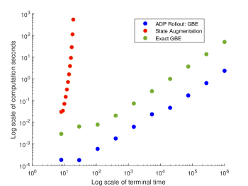
Figure 1: Log log graph showing computation time for solving MSOP (39) using state augmentation (red points), via exactly solving GBE (green points), and via approximately solving the GBE using the rollout (blue points) algorithm versus the terminal time of the problem.

4.1 Approximate Dynamic Programming Using The GBE

Rather than solving the MSOP (39) exactly using the GBE, as we did in the previous section, we now use an Approximate Dynamic Programming (ADP)/Reinforcement Learning (RL) algorithm to heuristically solve the MSOP and numerically show these algorithms can result in lower computational times when compared to methods that solve the GBE exactly. This demonstrates that MSOP’s with monotonically backward separable cost functions can be heuristically solved using the same methods developed in the ADP literature with the aid of the methodology developed in this paper.

Typically ADP methods use parametric function fitting (neural networks, linear combinations of basis functions, decision tree’s, etc) to approximate the value function from data. The approximated value function is then used to synthesize a sub-optimal input sequence. To see how this works, suppose an ADP algorithm constructs some approximate value function, denoted $\tilde{V}(x,t)$, then an approximate optimal input sequence, $\mathbf{\tilde{u}}=(\tilde{u}(0),...,\tilde{u}(T))$, can be constructed by solving

$$\tilde{u}(k)\in\arg\inf_{u\in\Gamma_{\tilde{x}(k),k}}\bigg{\{}\phi_{t}(\tilde{x}(k),u,\tilde{V}(f(\tilde{x}(k),u,k),k+1))\bigg{\}}$$

$$\hskip 113.81102pt\text{ for }k\in\{0,...,T-1\}.$$

$$\tilde{x}(0)=x_{0},\quad\tilde{x}(k+1)=f(\tilde{x}(k),\tilde{u}(k),k)$$

$$\hskip 113.81102pt\text{ for }k\in\{0,...,T-1\}.$$ (42)

One way to obtain an approximate value function, $\tilde{V}$, is to use the rollout algorithm found in the textbook [2]. This algorithm supposes a base policy is known $\mu_{base}:\mathbb{R}^{n}\times\mathbb{N}\to U$ and approximates the value function as follows

$$\tilde{V}(x,t)= \phi_{t}(x(t),u(t),\phi_{t+1}(x(t+1),u(t+1),...\phi_{T}(x(T))...)),$$

$$\text{where }x(t)=x\text{ and for all }s\in\{t,...,T-1\},$$

$$x(s+1)=f(x(s),u(s),t),\text{ }u(s)=\mu_{base}(x(s),s).$$

Using the base policy $\mu_{base}(x,t)=\begin{cases}1\text{ if }t/4\in\mathbb{N}\\ 0.5\text{ otherwise}\end{cases}$ we used the rollout algorithm to solve the MSOP (39) for terminal times $T=8$ to $10^{6}$. Computation times are plotted as the blue points in Figure 1 showing better performance than solving the GBE exactly or using state augmentation.

5 Application: Path Planning And Obstacle Avoidance

In this section we design a full state feedback controller (Markov Policy) for a discrete time dynamical system with the objective of reaching a target set in minimum time while avoiding moving obstacles.

5.1 MSOP’s For Path Planning

We say the MSOP, associated with tuple $\{J,f,\{X_{t}\}_{0\leq t\leq T},U,T\}$, defines a Path Planning DP problem if

• $J(\mathbf{u},\mathbf{x})=\min\bigg{\{}\inf\bigg{\{}t\in[0,T]:x(t)\in S\bigg{\}},T\bigg{\}}$.

• $S=\{x\in\mathbb{R}^{n}:g(x)<0\}$, where $g:\mathbb{R}^{n}\to\mathbb{R}$.

• $X_{t}=\mathbb{R}^{n}/(\cup_{i=1}^{N}O_{t,i})$, where $O_{t,i}=\{x\in\mathbb{R}^{n}:h_{t,i}(x)<0\}$ and $h_{t,i}:\mathbb{R}^{n}\to\mathbb{R}$.

• There exits a feasible solution, $(\mathbf{u},\mathbf{x})$, to the MSOP (2) associated with the tuple $\{J,f,\{X_{t}\}_{0\leq t\leq T},U,T\}$ such that $x(k)\in S$ for some $k\in\{0,...,T\}$.

Clearly, solving the MSOP (2) associated with a path planning problem tuple, $\{J,f,\{X_{t}\}_{0\leq t\leq T},U,T\}$, is equivalent to finding the input sequence that drives a discrete time system, governed by the vector field $f$, to a target $S$ in minimum time while avoiding the moving obstacles, represented as sets $O_{t,i}\subset\mathbb{R}^{n}$. Moreover, as shown in Example 4, the cost function $J$ is a naturally forward separable function (Defn. 3).

5.2 Path Planning for Dubin’s Car

We now solve the path planning problem with dynamics as defined in [23]; also known as the Dubin’s car dynamics.

$$f\left(x,u,t\right)=\left[x_{1}+v\cos(x_{3}),x_{2}+v\sin(x_{3}),x_{3}+\frac{v}{L}\tan(u)\right]^{T},$$ (43)

where $(x_{1},x_{2})\in\mathbb{R}^{2}$ is the position of the car, $x_{3}\in\mathbb{R}$ denotes the angle the car is pointing, $u\in\mathbb{R}$ is the steering angle input, $v\in\mathbb{R}$ is the fixed speed of the car, and $L$ is a parameter that determines the turning radius of the car.

We solve the path planning problem using a discretization scheme, similar to [12]; such discretization schemes are known to be parallelizable [24]. The target set, obstacles, state space, and input constraint sets are given by

$$S =\{(x_{1},x_{2})\in\mathbb{R}^{2}:-0.25<x_{1}-0.75<0.25,$$

$$\hskip 113.81102pt-0.25<x_{2}+0.75<0.25\}$$

$$O_{t,i} =\{(x_{1},x_{2})\in\mathbb{R}^{2}:(x_{1}-X_{i})^{2}+(x_{2}-Y_{i})^{2}-R_{i}^{2}<0\}$$

$$\hskip 28.45274pt\text{for }i\in\{1,...,15\}\text{ and }t\in\{0,...,T\}$$

$$X_{t}=[-1,1]^{2}\times\mathbb{R}\text{ for }t\in\{0,...,T\},\quad U=[-1,1],$$

where $X,Y,R\in\mathbb{R}^{15}$ are randomly generated vectors. The parameters of the system are set to $v=0.1$ and $L=1/6$.

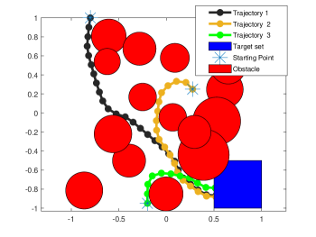
Figure 2: Graph showing approximate optimal trajectories, shown as the gold, black and green curves, with dynamics given in Eqn. (43) and the goal of reaching the target set, shown as the blue square, while avoiding obstacles, shown as red circles.

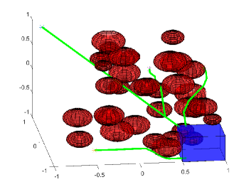
Figure 3: Graph showing approximate optimal trajectories, shown as the green curves, with dynamics given in Eqn. (44) and the goal of reaching the target set, shown as the blue cube, while avoiding obstacles, shown as red spheres.

Figure 2 shows three approximately optimal state sequences starting from different initial conditions. These state sequences are found by numerically solving the GBE (17), where $\{\phi_{t}\}_{t=0}^{T}$ are as in Example 4. To numerically solve the GBE (17) the state space, $X_{t}\subset\mathbb{R}^{3}$, is discretized as a $60\times 60\times 60$-grid between $[-1,1]^{2}\times[0,2\pi]$ and the input space, $U\subset\mathbb{R}$, is discretized as $100$ grid points within $[-1,1]$. The first state sequence was chosen to have initial condition $[-0.8,1,-0.55\pi]^{T}\in\mathbb{R}^{3}$ (the furthest of the three trajectories from the target) and took $25$ steps to reach its goal. The second state sequence was chosen to have initial condition $[0.275,0.25,0.75\pi]^{T}\in\mathbb{R}^{3}$; in this case as $x_{3}(0)=0.75\pi$ Dunbin’s car initially is directed towards the top left corner. The input sequence successfully turns the car downwards between two obstacles and into the target set, taking $18$ steps. The third trajectory was chosen to have initial condition $[-0.2,0.95,0.5\pi]^{T}\in\mathbb{R}^{3}$-starting very closely to an obstacle facing upwards. This trajectory had to use the full turning radius of the car to navigate around the obstacle towards the target set and took $10$ steps.

5.3 Path Planning in 3D

We now solve a three dimensional path planning problem with dynamics given by

$$f\left(x,u,t\right)=[x_{1}+u_{1},x_{2}+u_{2},x_{3}+u_{3}]^{T}.$$ (44)

The target set, obstacles, state space and input constraint set were respectively are given by

$$S=\{(x_{1},x_{2},x_{3})\in\mathbb{R}^{2}:-0.25<x_{1}-0.75<0.25,$$

$$\quad-0.25<x_{2}+0.75<0.25,-0.25<x_{2}+0.75<0.25\}$$

$$O_{t,i}=\{(x_{1},x_{2},x_{3})\in\mathbb{R}^{3}:(x_{1}-A_{i}-\alpha_{i}t)^{2}+(x_{2}-B_{i}-\beta_{i}t)^{2}$$

$$+(x_{2}-C_{i}-\gamma_{i}t)^{2}-R_{i}^{2}<0\}\text{ for }i\in\{1,...,35\},t\in\{0,...,T\}$$

$$X_{t}-[-1,1]^{3}\text{ for }t\in\{0,...,T\},\qquad U=[-0.05,0.05]^{3},$$

where $A,B,C,\alpha,\beta,\gamma,R\in\mathbb{R}^{35}$ are randomly generated vectors. Note, when $\alpha,\beta,\gamma$ are non-zero the center of the spherical obstacles moves with time. For presentation purposes in this paper we consider stationary obstacles, selecting $\alpha=\beta=\gamma=0$, however, a downloadable .gif file showing the numerical solution for moving obstacles can be found at [16].

This path planning problem can be numerically solved by computing the solution to the GBE (17) using $\{\phi_{t}\}_{t=0}^{T}$ as given in Example 4. To numerically solve the GBE (17) we discretized the state and input space, $X_{t}\subset\mathbb{R}$ and $U\subset\mathbb{R}^{3}$, as a $40\times 40\times 40$ uniform grid on $[-1,1]^{3}$ and a $5\times 5\times 5$ uniform grid on $[-0.05,0.05]^{3}$ respectively. Figure 3 shows four optimal state sequences, shown as green lines, starting from various initial conditions. All trajectories successfully avoid the obstacles, represented as red spheres, and reach the target set, shown as a blue cube.

GPU Implementation All DP methods involving discretization fall prey to the curse of dimensionality, where the number of points required to sample a space increases exponentially with respect to the dimension of the space. For this reason solving MSOP’s in dimensions greater than three can be computationally challenging. Fortunately, our discretization approach to solving the GBE (17), can be parallelized at each time-step. To improve the scalability of the proposed approach, we have therefore constructed in Matlab a GPU accelerated DP algorithm for solving the 3D path planning problem. This code is available for download at Code Ocean [13].

6 Application: Maximal Invariant Sets

The Finite Time Horizon Maximal Invariant Set (FTHMIS) is the largest set of initial conditions such that there exists an input sequence that produces a feasible state sequence over a finite time period. Computation of the maximal robust invariant sets over infinite time horizons was considered in [32]. Before we define the FTHMIS we introduce some notation.

For $f:\mathbb{R}^{n}\times\mathbb{R}^{m}\times\mathbb{N}\to\mathbb{R}^{n}$ we say the map $\rho_{f}:\mathbb{R}^{n}\times\mathbb{R}\times\mathbb{R}^{m\times(T-1)}\to\mathbb{R}^{n}$ is the solution map associated with $f$ if the following holds for all $(x_{0},t,\mathbf{u})\in\mathbb{R}^{n}\times\{0,...,T\}\times\mathbb{R}^{m\times(T-1)}$

$$\rho_{f}(x_{0},t,\mathbf{u})=x(t),$$

where $\mathbf{u}=(u(0),...,u(T-1))$, $x(k+1)=f(x(k),u(k),k)$ for all $k\in\{0,..,k-1\}$, and $x(0)=x_{0}$.

Definition 17.

For $f:\mathbb{R}^{n}\times\mathbb{R}^{m}\times\mathbb{N}\to\mathbb{R}^{n}$, $X_{t}\subseteq\mathbb{R}^{n}$, $U\subset\mathbb{R}^{m}$, $T\in\mathbb{N}$, and $\mathcal{A}_{t}\subseteq\mathbb{R}^{n}$ we define the Finite Time Horizon Maximal Invariant Set (FTHMIS), denoted by $\mathcal{R}$, by

$$\mathcal{R}:= \{x_{0}\in\mathbb{R}^{n}:\text{there exists }\mathbf{u}\in\Gamma_{x_{0},[0,T-1]}\text{ such that }$$

$$\hskip 56.9055pt\rho_{f}(x_{0},t,\mathbf{u})\in\mathcal{A}_{t}\text{ for all }t\in\{0,...,T\}\},$$

where the notation $\Gamma_{x_{0},[0,T-1]}$ is as in Eqn. (9).

We next show that the sublevel set of the value function associated with a certain MSOP can completely characterize the FTHMIS.

Theorem 18.

Consider the sets $\mathcal{A}_{t}=\{x\in\mathbb{R}^{n}:g_{t}(x)<0\}$, where $g_{t}:\mathbb{R}^{n}\to\mathbb{R}$. Suppose $V$ is a value function associated with the MSOP, defined by the tuple $\{J,f,\{X_{t}\}_{0\leq t\leq T},U,T\}$, where $J(\mathbf{u},\mathbf{x})=\max_{0\leq k\leq T}{g_{k}(x(k))}$. Then

$$\mathcal{R}=\{x\in\mathbb{R}^{n}:V(x,0)<0\},$$ (45)

where the set $\mathcal{R}\subset\mathbb{R}^{n}$ is the FTHMIS as in Defn. 17.

The function $J(\mathbf{u},\mathbf{x})=\max_{0\leq k\leq T}{g_{k}(x(k))}$ is monotonically backward separable as shown in Example 1 using representation maps given by

$$\phi_{i}(x,u,z) =\max\{g_{i}(x),z\}\text{ for all }i\in\{0,..,T-1\}$$

$$\phi_{T}(x) =g_{T}(x).$$

Therefore by Defn. 7 any value function, $V:\mathbb{R}^{n}\to\mathbb{R}$, associated with $\{J,f,\{X_{t}\}_{0\leq t\leq T},U,T\}$ satisfies

$$V(x,T)=g_{T}(x)\text{ for all }x\in X_{T},$$ (46)

and for all $t\in\{0,1,..,T-1\}$ and $x\in X_{t}$

$$V(x,t)=\inf_{\mathbf{u}\in\Gamma_{x,[0,T-1]}}\max_{t\leq k\leq T}{g_{k}(\rho_{f}(x,k,\mathbf{u}))}.$$ (47)

We will first show that $\mathcal{R}\subseteq\{x\in\mathbb{R}^{n}:V(x,0)<0\}$. Let $x_{0}\in\mathcal{R}$ then by Defn. 17 there exists $\mathbf{u}_{0}\in\Gamma_{x_{0},[0,T-1]}$ such that

$$\rho_{f}(x_{0},t,\mathbf{u}_{0})\in\mathcal{A}_{t}\quad\text{for all }t\in\{0,...,T\}.$$

As $\mathcal{A}_{t}=\{x\in\mathbb{R}^{n}:g_{t}(x)<0\}$ we deduce from the above equation that

$$g_{t}(\rho_{f}(x_{0},t,\mathbf{u}_{0}))<0\quad\text{for all }t\in\{0,...,T\}.$$ (48)

Therefore,

$$V(x_{0},0) =\inf_{\mathbf{u}\in\Gamma_{x_{0},[0,T-1]}}\max_{0\leq k\leq T}{g_{k}(\rho_{f}(x_{0},k,\mathbf{u}))}$$

$$\leq\max_{0\leq k\leq T}{g_{k}(\rho_{f}(x_{0},k,\mathbf{u}_{0}))}<0,$$

where the second inequality follows by Eqn. (48). We therefore deduce $x_{0}\in\{x\in\mathbb{R}^{n}:V(x,0)<0\}$ and hence $\mathcal{R}\subseteq\{x\in\mathbb{R}^{n}:V(x,0)<0\}$.

We next show $\{x\in\mathbb{R}^{n}:V(x,0)<0\}\subseteq\mathcal{R}$. Let $x_{0}\in\{x\in\mathbb{R}^{n}:V(x,0)<0\}$ then,

$$\inf_{\mathbf{u}\in\Gamma_{x_{0},[0,T-1]}}\max_{0\leq k\leq T}{g_{k}(\rho_{f}(x_{0},k,\mathbf{u}))}=V(x_{0},0)<0.$$

Therefore as the above inequality is strict, there exists some $\varepsilon>0$ such that

$$\inf_{\mathbf{u}\in\Gamma_{x_{0}}}\max_{0\leq k\leq T}{g_{k}(\rho_{f}(x_{0},k,\mathbf{u}))}=V(x_{0},0)<-\varepsilon.$$ (49)

By the definition of the infimum for any $\delta>0$ there exits $\mathbf{w}\in\Gamma_{x_{0},[0,T-1]}$ such that

$$\max_{0\leq k\leq T}{g_{k}(\rho_{f}(x_{0},k,\mathbf{w}))} <\inf_{\mathbf{u}\in\Gamma_{x_{0},[0,T-1]}}\max_{0\leq k\leq T}{g_{k}(\rho_{f}(x_{0},k,\mathbf{u}))}+\delta.$$ (50)

Hence by letting $0<\delta<\varepsilon$ we get

$$\max_{0\leq k\leq T}{g_{k}(\rho_{f}(x_{0},k,\mathbf{w}))} <\inf_{\mathbf{u}\in\Gamma_{x_{0},[0,T-1]}}\max_{0\leq k\leq T}{g_{k}(\rho_{f}(x_{0},k,\mathbf{u}))}+\delta$$

$$<-\varepsilon+\delta<0,$$ (51)

where the first inequality follows by Eqn. (50), the second inequality follows from Eqn. (49), and the third inequality follows from selecting $\delta<\varepsilon$.

Therefore by Eqn. (51) there exists $\mathbf{w}\in\Gamma_{x_{0},[0,T-1]}$ such that $\max_{0\leq k\leq T}g_{k}(\rho_{f}(x_{0},k,\mathbf{w}))<0$. We now deduce that for any $t\in\{0,...,T\}$

$$g_{t}(\rho_{f}(x_{0},t,\mathbf{w}))\leq\max_{0\leq k\leq T}g_{k}(\rho_{f}(x_{0},k,\mathbf{w}))<0.$$

Thus $\rho_{f}(x_{0},t,\mathbf{u}_{0})\in\mathcal{A}_{t}$, implying $x_{0}\in\mathcal{R}$. Therefore $\{x\in\mathbb{R}^{n}:V(x,0)<0\}\subseteq\mathcal{R}$. $\blacksquare$

6.1 Numerical Example: Maximal Invariant Sets

Value functions can characterize FTHMIS’s, as shown by Theorem 18. We now approximate a FTHMIS by computing a value function using a discretization scheme for solving the GBE (17) using $\{\phi_{t}\}_{t=0}^{T}$ as given in Example 1. Let us consider a discrete time switching system, whose Robust Maximal Invariant Set (RMIS) was previously computed in [32]:

$$f(x,u,t) =\begin{cases}\begin{bmatrix}x_{1}\\ (0.5+u)x_{1}-0.1x_{2}\end{bmatrix}\text{ if }1-(x_{1}-1)^{2}-x_{2}^{2}\leq 0\\ \begin{bmatrix}x_{2}\\ 0.2x_{1}-(0.1+u)x_{2}+x_{2}^{2}\end{bmatrix}\text{ otherwise}.\end{cases}$$ (52)

We now compute the FTHMIS, denoted by $\mathcal{R}$, associated with

$$\mathcal{A}_{t} =\{x\in\mathbb{R}^{2}:g_{t}(x)\leq 0\}\text{ for all }t\in\{0,..,T\},$$

$$g_{t}(x) =\left(x_{1}-\frac{(t-1)}{4}\right)^{2}+\left(x_{2}-\frac{(t+1)}{4}\right)^{2}-1.5,$$

$$X_{t} =[-1,1]^{2}\text{ for all }t\in\{0,..,T\},$$

$$U =\{u\in\mathbb{R}:u^{2}-0.01\leq 0\},\quad T=4.$$

Figure 4 shows the FTHMIS, $\mathcal{R}$, found by using a discretization scheme to solve the GBE (17) for $5\times 5$ state grid points in $[-1,1]^{2}$. To represent $\mathcal{R}$ in $\mathbb{R}^{2}$, once the value function, $V$, is found at each grid point a polynomial function is fitted and its zero-sublevel set, shown as the orange shaded region, approximately gives $\mathcal{R}$.

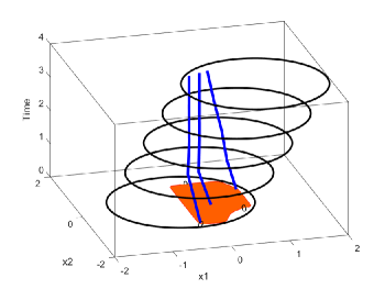
Figure 4: Figure showing an approximation of $L(V,0):=\{x\in\mathbb{R}^{n}:V(x,0)\leq 0\}$, shown in the shaded orange region, where $V$ is the value function of the MSOP associated with Eqn. (52). The z-axis represents time and the black circular lines represent the boundary of $\mathcal{A}_{t}$ for $t=1,2,3,4$. Three sample trajectories, shown in blue, start in $L(V,0)$ and remain in the sets $\mathcal{A}_{t}$ for the time-steps $t=1,2,3,4$; giving numerical evidence that $L(V,0)$ is indeed an approximation of the FTHMIS.

7 Conclusion

For MSOP’s with monotonically backward separable cost functions we have derived necessary and sufficient conditions for solutions to be optimal. We have shown that by solving the Generalized Bellman’s Equation (GBE) one can derive an optimal input sequence. Furthermore, we have demonstrated the GBE can be numerically solved using a discretization scheme and Approximate Dynamic Programing (ADP) techniques such as Rollout. We have shown our numerical methods can solve current practical problems of interest; such as path planning and the computation of maximal invariant sets.

Morgan Jones received the B.S. and Mmath in mathematics from The University of Oxford, England in 2016. He is a research associate with Cybernetic Systems and Controls Laboratory (CSCL) at ASU. His research primarily focuses on the analysis of nonlinear ODE’s and Dynamic Programming.

Matthew M. Peet received the B.S. degree in physics and in aerospace engineering from the University of Texas, Austin, TX, USA, in 1999 and the M.S. and Ph.D. degrees in aeronautics and astronautics from Stanford University, Stanford, CA, in 2001 and 2006, respectively. He was a Postdoctoral Fellow at INRIA, Paris, France from 2006 to 2008. He was an Assistant Professor of Aerospace Engineering at the Illinois Institute of Technology, Chicago, IL, USA, from 2008 to 2012. Currently, he is an Associate Professor of Aerospace Engineering at Arizona State University, Tempe, AZ, USA. Dr. Peet received a National Science Foundation CAREER award in 2011.

References

• [1] Richard Bellman. Dynamic programming. Science, 153(3731):34–37, 1966.
• [2] Dimitri P Bertsekas. Dynamic programming and optimal control, volume 1. Athena scientific Belmont, MA, 1995.
• [3] Dimitri P Bertsekas. Abstract dynamic programming. Athena Scientific, 2018.
• [4] Raghvendra V Cowlagi and Panagiotis Tsiotras. Hierarchical motion planning with dynamical feasibility guarantees for mobile robotic vehicles. IEEE Transactions on Robotics, 28(2):379–395, 2011.
• [5] Stuart E Dreyfus. An appraisal of some shortest-path algorithms. Operations research, 17(3):395–412, 1969.
• [6] Willem Esterhuizen, Tim Aschenbruck, and Stefan Streif. On maximal robust positively invariant sets in constrained nonlinear systems. arXiv preprint arXiv:1904.01985, 2019.
• [7] Giorgio Gallo and Stefano Pallottino. Shortest path algorithms. Annals of operations research, 13(1):1–79, 1988.
• [8] Philip E Gill, Walter Murray, and Michael A Saunders. Snopt: An sqp algorithm for large-scale constrained optimization. SIAM review, 47(1):99–131, 2005.
• [9] Keith Glover and John C Doyle. State-space formulae for all stabilizing controllers that satisfy an $h_{\infty}$-norm bound and relations to relations to risk sensitivity. Systems & control letters, 11(3):167–172, 1988.
• [10] David Jacobson. Optimal stochastic linear systems with exponential performance criteria and their relation to deterministic differential games. IEEE Transactions on Automatic control, 18(2):124–131, 1973.
• [11] Morgan Jones and Matthew M Peet. Solving dynamic programming with supremum terms in the objective and application to optimal battery scheduling for electricity consumers subject to demand charges. In Conference on Decision and Control (CDC), pages 1323–1329. IEEE, 2017.
• [12] Morgan Jones and Matthew M Peet. Extensions of the dynamic programming framework: Battery scheduling, demand charges, and renewable integration. arXiv preprint arXiv:1812.00792, 2018.
• [13] Morgan Jones and Matthew M Peet. GPU accelerated 3D dynamic programming path planning and obstacle avoidance. https://codeocean.com/capsule/3639299/, 2019.
• [14] Morgan Jones and Matthew M Peet. Relaxing the Hamilton Jacobi Bellman equation to construct inner and outer bounds on reachable sets. arXiv preprint arXiv:1903.07274, 2019.
• [15] Morgan Jones and Matthew M Peet. Using SOS and sublevel set volume minimization for estimation of forward reachable sets. arXiv preprint arXiv:1901.11174, 2019.
• [16] Morgan Jones and Matthew M Peet. Path planning animation. ResearchGate DOI:10.13140/RG.2.2.20466.32968, 2020.
• [17] Duan Li. Multiple objectives and non-separability in stochastic dynamic programming. International Journal of Systems Science, 21(5):933–950, 1990.
• [18] Duan Li and Yacov Y Haimes. Multilevel methodology for a class of non-separable optimization problems. International Journal of Systems Science, 21(11):2351–2360, 1990.
• [19] Duan Li and Yacov Y Haimes. New approach for nonseparable dynamic programming problems. Journal of Optimization Theory and Applications, 64(2):311–330, 1990.
• [20] Duan Li and Yacov Y Haimes. Extension of dynamic programming to nonseparable dynamic optimization problems. Computers & Mathematics with Applications, 21(11-12):51–56, 1991.
• [21] Qinming Liu, Ming Dong, Wenyuan Lv, and Chunming Ye. Manufacturing system maintenance based on dynamic programming model with prognostics information. Journal of Intelligent Manufacturing, 30(3):1155–1173, 2019.
• [22] Yun-Hui Liu and Suguru Arimoto. Path planning using a tangent graph for mobile robots among polygonal and curved obstacles. The International Journal of Robotics Research, 11(4):376–382, 1992.
• [23] John Maidens, Axel Barrau, Silvère Bonnabel, and Murat Arcak. Symmetry reduction for dynamic programming. Automatica, 97:367–375, 2018.
• [24] John Maidens, Andrew Packard, and Murat Arcak. Parallel dynamic programming for optimal experiment design in nonlinear systems. In Conference on Decision and Control (CDC), pages 2894–2899. IEEE, 2016.
• [25] Eran Rippel, Aharon Bar-Gill, and Nahum Shimkin. Fast graph-search algorithms for general-aviation flight trajectory generation. Journal of Guidance, Control, and Dynamics, 28(4):801–811, 2005.
• [26] Andrzej Ruszczyński. Risk-averse dynamic programming for markov decision processes. Mathematical programming, 125(2):235–261, 2010.
• [27] Andrey V Savkin and Michael Hoy. Reactive and the shortest path navigation of a wheeled mobile robot in cluttered environments. Robotica, 31(2):323, 2013.
• [28] Alexander Shapiro. On a time consistency concept in risk averse multistage stochastic programming. Operations Research Letters, 37(3):143–147, 2009.
• [29] Alexander Shapiro and Kerem Ugurlu. Decomposability and time consistency of risk averse multistage programs. Operations Research Letters, 44(5):663–665, 2016.
• [30] Zheming Wang, Raphaël M Jungers, and Chong-Jin Ong. Computation of the maximal invariant set of discrete-time systems subject to quasi-smooth non-convex constraints. arXiv preprint arXiv:1912.09727, 2019.
• [31] Junfei Xie, Lei Jin, and Luis Rodolfo Garcia Carrillo. Optimal path planning for unmanned aerial systems to cover multiple regions. In AIAA Scitech 2019 Forum, page 1794, 2019.
• [32] Bai Xue and Naijun Zhan. Robust invariant sets computation for switched discrete-time polynomial systems. arXiv preprint arXiv:1811.11454, 2018.
• [33] Xiangrui Zeng and Junmin Wang. Globally energy-optimal speed planning for road vehicles on a given route. Transportation Research Part C: Emerging Technologies, 93:148–160, 2018.