Shapley Supercluster Survey: mapping the dark matter distribution

Abstract

We present a 23 deg² weak gravitational lensing survey of the Shapley supercluster core and its surroundings using $gri$ VST images as part of the Shapley Supercluster Survey (ShaSS). This study reveals the overall matter distribution over a region containing 11 clusters at $z{\sim}0.048$ that are all interconnected, as well as several ongoing cluster-cluster interactions. Galaxy shapes have been measured by using the Kaiser-Squires-Broadhurst method for the $g$- and $r$-band images and background galaxies were selected via the $gri$ colour-colour diagram. This technique has allowed us to detect all of the clusters, either in the $g$-band or $r$-band images, although at different $\sigma$ levels, indicating that the underlying dark matter distribution is tightly correlated with the number density of the member galaxies. The deeper $r$-band images have traced the five interacting clusters in the supercluster core as a single coherent structure, confirmed the presence of a filament extending North from the core, and have revealed a background cluster at $z{\sim}0.17$. We have measured the masses of the four richest clusters (A3556, A3558, A3560 and A3562) in the two-dimensional shear pattern, assuming a spherical Navarro-Frenk-White (NFW) profile and obtaining a total mass of $\mathcal{M}_{\rm ShaSS,WL}{=}1.56^{+0.81}_{-0.55}{\times}10^{15\,}{\rm M}_{\odot}$, which is consistent with dynamical and X-ray studies. Our analysis provides further evidence of the ongoing dynamical evolution in the ShaSS region.

1 Introduction

Large-scale optical and spectroscopic explorations such as the Sloan Digital Sky Survey (York et al., 2000) have revealed the complex structures of the Universe – galaxy clusters, filaments and voids. Superclusters represent the vastest coherent structures in the Universe, extending up to $\sim$100 across as observed in the wide optical surveys (e.g. Einasto et al., 2011). The observation of superclusters was often considered a challenge to the hierarchical structure formation paradigm since such extremely vast overdense structures, but also the largest voids, are not reproduced by the $N$-body simulations. However, new techniques to analyse $N$-body simulations (e.g. Yaryura et al., 2011; Higuchi & Inoue, 2019) obtained non-zero probabilities of identifying such peculiar systems (overdense and underdense) within redshift surveys. Recent numerical simulations (Einasto et al., 2019) showed that the stability of size and number of superclusters during their evolution are important properties of the cosmic web and that the number density of the superclusters thus constrains the cosmological models. Also, these structures are still collapsing with galaxy clusters and groups frequently interacting and merging, enhancing the effects of the environment on galaxy evolution. These effects are amplified in the supercluster high-density cores, which are gravitationally-bound (Einasto et al., 2016) and anticipated to become the most massive virialized structures in the distant future. This implies that galaxy properties and the wider supercluster evolution are strongly related (e.g. Gray et al., 2009; Lubin et al., 2009; Mei et al., 2012; Merluzzi et al., 2016; Galametz et al., 2018; Einasto et al., 2018; Mahajan et al., 2018).

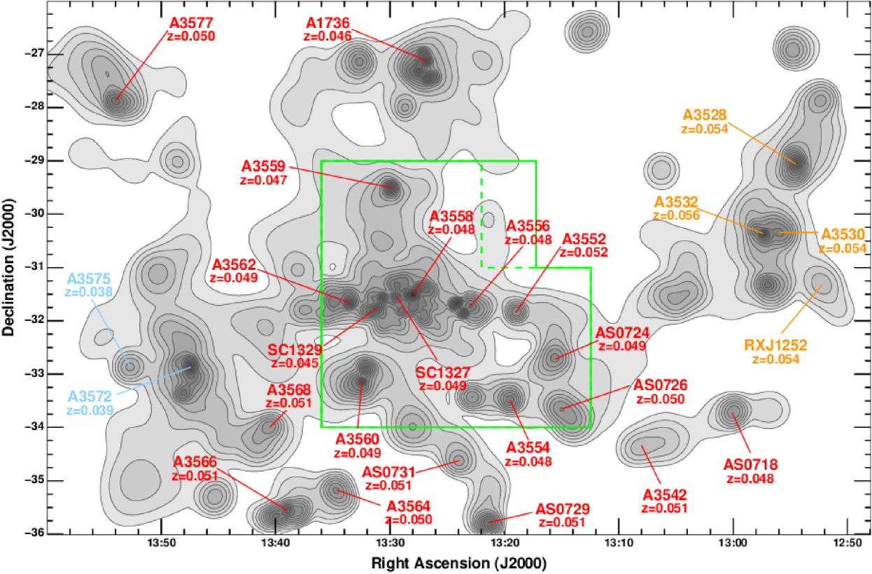
Figure 1: $K$-band luminosity-weighted density map of $0.035{\leq}z{<}0.060$ galaxies across the full extent of the Shapley Supercluster. $K$-band magnitudes are taken from the 2MASS Extended Source Catalog and combines redshifts from the previous wide-field spectroscopic surveys covering the region (6dFGRS; Jones et al., 2009; Quintana et al., 1997; Kaldare et al., 2003; Drinkwater et al., 2004; Proust et al., 2006; Cava et al., 2009). Abell clusters within the same redshift range are labelled, colour coded as: (red) recession velocities within 1 500 km s^-1 of the central cluster Abell 3558; (cyan) low-velocity extension $0.035{\leq}z{<}0.040$; (orange) high-velocity wing, $0.053{\leq}z{<}0.060$. The solid green box outlines the 23 deg² region covered by ShaSS, and the dashed green lines our 21 deg² AAOmega survey (see text).

Table 1: Properties of the 11 known X-ray galaxy clusters in the Shapley supercluster. The central velocities $\langle V_{\mathrm{h}}\rangle$, velocity dispersions $\sigma_{\nu}$, number of spectroscopic members within $r_{200}$ ($N_{\mathrm{z}}$), and $r_{200}$ radii (in Mpc) are all determined by Haines et al. (2018). ROSAT-based X-ray bolometric luminosities taken from de Filippis et al. (2005), except A 3559, A 3560 from Ettori et al. (1997). The last column lists the dynamical masses derived from the analysis of Haines et al. (2018).

Cluster	R.A.(J2000)	Dec.(J2000)	$\langle V_{\mathrm{h}}\rangle$		$\sigma_{\nu}$		$N_{\mathrm{z}}$	$r_{200}$	$L_{\mathrm{X,bol}}$	$\mathcal{M}_{\mathrm{dyn}}$
Name	[degrees]	[degrees]	[km s-1]		[km s-1]			[Mpc]	$10^{43}$[erg s${}^{-1}]$	$[10^{13}{\rm M}_{\odot}]$
AS 0724	198.863788	-32.710022	14 748$\,\pm\,$	74	410$\,\pm\,$	41	29	0.945	1.5	10.06$\,\pm\,$	3.02
AS 0726	198.655892	-33.764558	14 911$\,\pm\,$	94	603$\,\pm\,$	48	38	1.397	0.7	32.40$\,\pm\,$	7.74
Abell 3552	199.729560	-31.817560	15 777$\,\pm\,$	75	334$\,\pm\,$	42	19	0.769	0.4	5.41$\,\pm\,$	2.04
Abell 3554	199.881979	-33.488139	14 346$\,\pm\,$	66	602$\,\pm\,$	37	77	1.387	2.0	31.67$\,\pm\,$	5.84
Abell 3556	201.028020	-31.669858	14 396$\,\pm\,$	45	628$\,\pm\,$	31	257	1.447	1.7	35.94$\,\pm\,$	5.32
Abell 3558	201.986896	-31.495847	14 500$\,\pm\,$	39	1007$\,\pm\,$	25	867	2.319	66.8	148.16$\,\pm\,$	13.72
Abell 3559	202.462154	-29.514386	14 149$\,\pm\,$	63	521$\,\pm\,$	39	68	1.201	1.5	20.59$\,\pm\,$	4.62
Abell 3560	203.107354	-33.135989	14 739$\,\pm\,$	52	860$\,\pm\,$	32	304	1.981	11.7	92.29$\,\pm\,$	10.30
Abell 3562	203.402575	-31.670383	14 786$\,\pm\,$	53	769$\,\pm\,$	30	198	1.770	33.1	65.87$\,\pm\,$	7.71
SC 1327-312	202.448625	-31.602450	14 794$\,\pm\,$	38	535$\,\pm\,$	17	220	1.347	12.7	29.84$\,\pm\,$	2.84
SC 1329-313	202.913761	-31.807260	13 416$\,\pm\,$	49	373$\,\pm\,$	28	55	0.862	5.2	7.60$\,\pm\,$	1.71

The Shapley supercluster (SSC, $z\sim 0.05$) is the largest conglomeration of Abell clusters in the local Universe (see Fig. 1). At its heart there is a complex dense core consisting of five clusters forming a continuous filamentary structure 2 degrees ($\sim$8 Mpc; $H_{0}=70$ km s^-1 Mpc^-1) in extent, that is filled with hot gas as seen by both Planck and $XMM-Newton$ satellites (Planck Collaboration et al., 2014; Merluzzi et al., 2016). Across this central region dynamical studies, X-ray and radio observations showed evidence of multiple cluster-cluster interactions (e.g. Bardelli et al., 1998, 2000; Kull & Böhringer, 1999; Venturi et al., 2003; Giacintucci et al., 2005; Miller, 2005). Several attempts have also been undertaken to map the whole supercluster in order to determine its morphology and mass, as well as ascertain which portions of the supercluster were gravitationally bound (e.g. Reisenegger et al., 2000; Drinkwater et al., 2004; de Filippis et al., 2005; Proust et al., 2006; Muñoz & Loeb, 2008). The supercluster resides in the direction of the Cosmic Microwave Background (CMB) dipole anisotropy. Quintana et al. (1995) showed that the gravitational pull of the supercluster may account for $25\%$ of the peculiar velocity of the Local Group required to explain the anisotropy and their mass would be dominated by inter-cluster dark matter in that case, while the optical flux distribution lies $\sim 25$ degrees away from the CMB dipole. However, due to a lack of robust estimates of the SSC mass, the relevance of its gravitational pull upon the high peculiar velocity (${\sim}$600 km s^-1) of the Local Group relative to the Hubble Flow remains an open issue (Raychaudhury, 1989; Kocevski et al., 2004; Courtois et al., 2017). An order of magnitude estimate of the SSC mass was provided by Reisenegger et al. (2000), by means of a dynamical analysis based on supercluster member galaxies. They estimated the mass of the central region within $8h^{-1}$Mpc of A 3558 to be $\mathcal{M}\sim 10^{16}h^{-1}{\rm M}_{\odot}$.

Although the previous studies were fundamental to demonstrate the complex dynamical status of the SSC, the lack of accurate and homogeneous multi-band imaging and spectroscopic coverage across such an extended structure prevented, among other things, a quantitative description of the supercluster environment from filaments to cluster cores and a robust mass estimate.

With all this in mind we have carried out the Shapley Supercluster Survey (ShaSS, Merluzzi et al., 2015), delivering high-quality optical and near-infrared imaging across a contiguous 23 deg² (260 $h^{-2}_{70}$Mpc²) region centred on the supercluster core. The survey includes nine Abell clusters (A 3552, A 3554, A 3556, A 3558, A 3559, A 3560, A 3562, AS 0724, AS 0726) and two poor clusters (SC 1327-312, SC 1329-313) whose redshifts all lie within 1 500 km s^-1 of Abell 3558 at $z=0.048$ (see solid green box in Fig. 1 and refer for details to Merluzzi et al., 2015). The parameters of the clusters are given in Table 1 (see Haines et al., 2018).

The main objective of the ShaSS project is to investigate the role of cluster-scale mass assembly on the evolution of galaxies, mapping the effects of the environment in the cluster outskirts and along the filaments with the aim of identifying the very first interactions between galaxies and their environment. In order to achieve this goal it is crucial to reveal the structure, i.e. to obtain detailed maps of the dark matter and baryonic matter distributions (galaxies, intra-cluster medium), combining galaxy number and stellar mass density, weak lensing, X-ray and dynamical analyses. In the present work we characterized the supercluster environment by means of weak lensing (WL) technique.

While we have been able to produce highly-detailed and complete two-dimensional density maps of the galaxy distribution across the Shapley supercluster (Haines et al., 2018) and the stellar mass content (Merluzzi et al., 2015), this stellar content is expected to only represent a relatively small fraction of the global mass of this region, in comparison to the hot X-ray emitting gas of the clusters and the wider dark matter component. More problematically, the relative fraction of baryonic component that is locked into stars and galaxies rather than hot gas, and the global mass-to-light ratios have been shown to vary significantly between galaxy groups and the most massive clusters, with galaxy groups much more efficient at converting the baryons into stars and producing light than clusters (e.g. Tully, 2005; Gonzalez et al., 2007, 2013). Thus it is no trivial matter to translate the galaxy distribution or stellar mass distribution to the wider mass distribution.

Weak gravitational lensing enables the overall mass distribution of clusters and superclusters to be directly measured without requiring us to make any assumptions regarding the dynamical state of the system (Einasto et al., 2003; Oguri et al., 2004). The tidal gravitational field of a cluster leads to the differential deflection of light coming from background galaxies, distorting them and producing a coherent shear signal on top of the random intrinsic ellipticities of individual galaxies. Measuring this coherent distortion pattern among the background galaxies enables the two-dimensional mass distribution of the cluster/supercluster to be mapped (e.g. Medezinski et al., 2010; Oguri et al., 2012; Umetsu et al., 2014). This technique is particularly powerful for those unvirialised regions beyond the cluster core, where traditional approaches based on galaxy dynamics or X-ray emission are no longer suitable. Weak lensing analyses have been used to detect filamentary structures connecting adjacent galaxy clusters (Heymans et al., 2008; Dietrich et al., 2012; Higuchi et al., 2014), or provide mass maps of merging cluster systems (e.g. Okabe & Umetsu, 2008; Jee et al., 2014).

In a previous study applying a lensing analysis to superclusters, we showed the correlation between the early-type galaxy distribution and WL density map in the central $\sim 1$ deg² region including A 3558 and SC 1327-312. We measured for the mass of A 3558 $\mathcal{M}_{500}=7.63_{-3.40}^{+3.88}\times 10^{14}$ M_⊙ consistent with that derived from the X-ray observations $\mathcal{M}_{500}=(4.62\pm 0.24)\times 10^{14}$ M_⊙ (Merluzzi et al., 2015). The agreement of the two independent measurements demonstrated the feasibility and effectiveness of the WL analysis which we will here extend and improve considering the whole ShaSS region.

Beyond deriving cluster masses using a complementary approach, the WL technique will enable us to further investigate the nature of the whole system, tracing the mass distribution outside of the cluster cores, as well as revealing possible background structures. In particular, in Haines et al. (2018) with the galaxy number density map and the dynamical analysis we established the existence of a stream of galaxies connecting A 3559 to the supercluster core. Moreover, the updated central redshifts and velocity dispersions of the 11 clusters confirmed that they all lie within 1300 km s^-1 of the central cluster A 3558. These 11 systems are all inter-connected and lie within a coherent sheet of galaxies that fills the entire survey region without gaps. Clear velocity caustics extend right to the survey boundary, indicating that the entire structure is gravitationally bound and in the process of collapse. All this invokes and supports a deeper examination.

The structure of the paper is organized as follows. Section 2 describes the main characteristics of the dataset. Section 3 introduces the basics of weak lensing and the methods of analysis. The shear measurement, background galaxies selection and fitting procedure are detailed in Section 4. Section 5 presents the results of the WL analysis which are discussed in Section 6. Lastly, Section 7 summarizes our findings.

We adopt the following cosmological parameters: the Hubble parameter $H_{0}=70$ km s^-1 Mpc^-1, the density parameter of total matter $\Omega_{\rm m}=0.3$, $\Omega_{\Lambda}=0.7$, spectral index $n_{s}=0.972$ and density fluctuation amplitude $\sigma_{8}=0.823$, assuming a flat FLRW cosmology. Otherwise, $h=H_{0}/100$.

2 The data

The ShaSS database consists of high-quality optical $ugri$ imaging acquired with OmegaCAM (Kuijken, 2011) on the 2.6m VLT Survey Telescope (VST, Capaccioli & Schipani, 2011) and near-infrared $K$-band imaging from the 4.1m Visible and Infrared Survey Telescope for Astronomy (VISTA), both taking advantage of the exceptional observing conditions available at Cerro Paranal in Chile. In addition, our $ad\,hoc$ spectroscopic survey carried out with the AAOmega spectrograph on the 3.9m Anglo Australian Telescope provides highly-complete and homogeneous redshift coverage across the full ShaSS region (see Haines et al., 2018).

The corrected OmegaCAM field of view of 1^∘x 1^∘ allows the whole ShaSS area to be covered with 23 VST fields, sampled at 0.21 arcsec-per-pixel corresponding to a sub-kiloparsec resolution at the supercluster redshift. Each of the contiguous ShaSS fields is observed in four bands, $u$ ($t_{\mathrm{exp}}$ = 2955 s), $g$ (1400 s), $r$ (2664 s), and $i$ (1000 s), reaching 5$\sigma$ (AB) magnitude limits of 24.4, 24.6, 24.1, and 23.3, respectively (see Merluzzi et al., 2015; Mercurio et al., 2015). The $r$-band images were to be acquired in the best seeing conditions with the aim of using these data for shear measurements and morphological classification. The median seeing in $r$-band is 0.6 arcsec, corresponding to 0.56 kpc $h^{-2}_{70}$ at $z=0.048$.

Table 2: List of the parameters from the $gri$ catalogues that were used to perform the WL analysis.

Parameter	Units	Description
$ID$		ShaSS identification
$RA$	deg	Right Ascension (J2000)
$DEC$	deg	Declination (J2000)
$MK$	mag	Kron magnitude
$EMK$	mag	Error on Kron magnitude
$MA_{15}$	mag	Aperture magnitude inside 1.5 arcsec diameter
$EMA_{15}$	mag	Error on aperture magnitude inside 1.5 arcsec diameter
$MPSF$	mag	Magnitude resulting from the PSF fitting
$EPSF$	mag	Error on magnitude resulting from the PSF fitting
$SG$		Star/galaxy separation
$HFF$		Halo fraction flag
$HF$		Halo flag value
$SFF$		Spike fraction flag
$SF$		Spike flag value

The VST images have been processed and photometrically calibrated using the VST-Tube pipeline (Grado et al., 2012), and the catalogue produced as described in Mercurio et al. (2015). In each band the complete catalogues contain a wealth of information. Table 2 lists the parameters from the catalogues that have been used for the WL analysis. Both the Kron magnitudes ($MK$, Kron, 1980) and the 1.5 arcsec aperture magnitudes ($MA_{15}$) were corrected for Galactic extinction following Schlafly & Finkbeiner (2011).

Since multiple reflections in the internal optics of OmegaCAM can produce complex image rings and ghosts (hereafter star haloes) near bright stars, we carefully traced the effects of such features on source detection (for details see Mercurio et al., 2015). In addition, the saturated stars with haloes also affect the images by producing spike features which are identified. The parameters $HFF$, $HF$, $SFF$, $SF$ in Table 2 are indicative of the robustness of the photometry. $HF$ ($SF$) greater than 0 marks that the source is at least partially affected by the halo (spike) of a bright star and indicates the star magnitudes (spike strength). While $HFF$ ($SFF$) measures the fraction of the source area affected by the halo (spike). Finally, the $SG$ parameter identifies galaxies ($SG=0$) and stars ($SG>0$). The saturated stars ($SG=9$) are also indicated. In the following analysis we excluded all the sources with HF or SF greater than 0, i.e. all the sources even marginally affected by haloes or spikes, as well as saturated stars.

The survey was designed to study the galaxy population down to $m^{\star}+6$ at supercluster redshift ($m_{r}^{\star}=15$ mag in AB magnitudes). With this precondition, we fixed the required depth in each band using typical galaxy colours at $z\sim 0.05$ according to stellar population models (e.g. Bruzual & Charlot, 2003). Further constraints were placed by (i) the morphological classification based on the $r$-band imaging which requires a signal-to-noise ratio about 100 and (ii) the plan to use $r$-band imaging for the WL analysis. This translates in photometric catalogues having different magnitude limits in the different bands, with the $r$-band catalogue including the fainter sources in the ShaSS field.

It follows that to maximize the number density of sources for the background galaxy selection (see Section 4) and the photometric redshift estimate we take advantage of the deeper $gri$ catalogues. The three catalogues have been cross-correlated using STILTS with the $r$-band catalogue as reference table and keeping only the sources detected in all the three bands.

The $g$-band imaging is generally used for the WL mass measurement presented here, together with the $gri$ catalogues and the spectroscopic catalogue. Although the $r$-band imaging is deeper, the $r$-band imaging was found to present significant distortions in some restricted regions, and thus the $g$-band imaging was used as an alternative source of shear measurements. For this reason, and to provide consistency checks across the wider WL maps, the WL analysis was carried out in both $r$ and $g$ bands.

The spectroscopic survey was carried out using the AAOmega multi-fiber spectrograph on the 3.9-m Anglo-Australian telescope, collecting redshift measurements for 4027 galaxies (Haines et al., 2018). Targets were selected from the VST images as having $i<18.0$ (AB) and WISE/W$1<15.5$ mag (Vega). There have also been multiple previous redshift surveys of the region, and combining these literature redshifts with our own, results in redshifts being known for 95% of all $i<18$, W$1<15.5$ galaxies (5689/6008) across the whole survey region. The redshift distribution of the non-SSC galaxies has the typical form of magnitude-limited samples (e.g. Jones et al., 2009), with a median redshift of 0.138 and 95% of galaxies within the range 0.014–0.295. This permits background structures connected to the WL peaks to be reliably identified and mapped in redshift-space out to $z\sim 0.3$.

3 Analysis methods

3.1 Navarro-Frenk-White model

Simulations and observational results revealed that the halo density profile is inversely proportional to the distance $r$ from the cluster centre inside a scale radius $r_{s}$, and proportional to $r^{-3}$ outside this radius. This profile is called NFW profile (Navarro et al., 1997), defined by

$$\rho(r)=\frac{\delta_{\mathrm{c}}\rho_{\mathrm{c}}}{r/r_{\mathrm{s}}(1+r/r_{\mathrm{s}})^{2}},$$ (1)

where $\rho_{\mathrm{c}}$ is the critical density of the Universe at the cluster redshift. The characteristic overdensity is described with the concentration parameter $c=r_{200}/r_{\mathrm{s}}$ by

$$\delta_{\mathrm{c}}=\frac{200}{3}\frac{c^{3}}{{\rm ln}\left(1+c\right)-c/\left(1+c\right)},$$ (2)

where $r_{200}$ is defined as the radius inside which the mass density of the halo is equal to 200 times the critical density. The scale radius can be derived from the mass of the halo $M_{200}$ and the concentration parameter as

$$r_{s}=\left(\frac{3M_{200}}{800\pi\rho_{\mathrm{c}}}\right)^{1/3}c.$$ (3)

Therefore, the density profile can be determined as a function of mass and concentration parameter when the halo redshift is known.

3.2 Concentration and mass relation

$N$-body simulations and observational results show that halo mass is correlated with the concentration parameter (Jing, 2000; Bullock et al., 2001; Zhao et al., 2009; Oguri et al., 2012; Umetsu et al., 2014). The concentration and mass relation (hereafter, c-M relation) can be modeled with four parameters $M_{\rm piv}$, $A$, $B$ and $C$ at a redshift of $z$ (Duffy et al., 2008) as

$$c=A\left(\frac{M_{200}}{M_{\rm piv}}\right)^{B}(1+z)^{C}.$$ (4)

In the following analysis, we used $M_{\rm piv}=2\times 10^{12}h^{-1}{\rm M}_{\odot}$, $A=7.85$, $B=-0.081$ and $C=-0.71$ which were obtained by fitting haloes in the $N$-body simulation (Duffy et al., 2008).

3.3 Lensing equations

The three-dimensional potential $\Phi(D_{\mathrm{d}}{\bf\theta},z)$ of a lens is related to the lensing potential $\psi({\bf\theta})$ on the sky plane as

$$\psi(\bm{\theta})=\frac{2D_{\mathrm{ds}}}{c^{2}D_{\mathrm{d}}D_{\mathrm{s}}}\int dz\Phi(D_{\mathrm{d}}\bm{\theta},z),$$ (5)

where $\bm{\theta}$ is a position vector on the sky plane and $c$ is the speed of light. $D_{\mathrm{d}}$, $D_{\mathrm{s}}$ and $D_{\mathrm{ds}}$ are respectively the angular diameter distances between the observer and the lens, the observer and the sources, and between the lens and the sources. Given the cluster properties, the convergence and shear for the NFW profile can be obtained as the derivatives of the lens potential. The potential is related to the shear as

$$\gamma_{1}(\bm{\theta})=\frac{1}{2}\left(\frac{\partial^{2}\psi(\bm{\theta})}{\partial\theta_{1}^{2}}-\frac{\partial^{2}\psi(\bm{\theta})}{\partial\theta_{2}^{2}}\right),$$ (6)

$$\gamma_{2}(\bm{\theta})=\frac{\partial^{2}\psi(\bm{\theta})}{\partial\theta_{1}\partial\theta_{2}}.$$ (7)

For spherically-symmetric objects, the direction of shear has only a tangential component. It is useful to define the tangential $\gamma_{+}$ and cross $\gamma_{\textrm{x}}$ components for $\gamma_{1}$ and $\gamma_{2}$ as

$$\left(\begin{array}[]{c}\gamma_{+}\\ \gamma_{\textrm{x}}\end{array}\right)=\left(\begin{array}[]{cc}\textrm{-cos}2\phi&\textrm{-sin}2\phi\\ \textrm{-sin}2\phi&\textrm{cos}2\phi\end{array}\right)\left(\begin{array}[]{c}\gamma_{1}\\ \gamma_{2}\end{array}\right),$$ (8)

where $\phi$ is the angle between the galaxy position and $\theta_{1}$ axis. The shear profile for the spherical symmetric NFW profile can be written as a function of the distance from the centre by (Wright & Brainerd, 2000; Bartelmann & Schneider, 2001)

$$\frac{r_{\mathrm{s}}\delta_{\mathrm{c}}\rho_{\mathrm{c}}}{\Sigma_{\mathrm{c}}}\left[\frac{8{\rm arctanh}\sqrt{(1+x)/(1-x)}}{x^{2}\sqrt{1-x^{2}}}+\frac{4}{x^{2}}{\rm ln\left(\frac{x}{2}\right)}\right.$$

$$\left.-\frac{2}{x^{2}-1}+\frac{4{\rm arctanh}\sqrt{(1-x)/(1+x)}}{(x^{2}-1)\sqrt{1-x^{2}}}\right]~{}~{}(x<1),$$

$$\gamma_{+}(x) = \frac{r_{\mathrm{s}}\delta_{\mathrm{c}}\rho_{\mathrm{c}}}{\Sigma_{\mathrm{c}}}\left[\frac{10}{3}+4{\rm ln}\left(\frac{1}{2}\right)\right]~{}~{}~{}~{}~{}~{}~{}~{}~{}~{}~{}~{}~{}~{}~{}~{}~{}~{}~{}(x=1),$$

$$\frac{r_{\mathrm{s}}\delta_{\mathrm{c}}\rho_{\mathrm{c}}}{\Sigma_{\mathrm{c}}}\left[\frac{8{\rm arctanh}\sqrt{(x-1)/(1+x)}}{x^{2}\sqrt{x^{2}-1}}+\frac{4}{x^{2}}{\rm ln\left(\frac{x}{2}\right)}\right.$$

$$\left.-\frac{2}{x^{2}-1}+\frac{4{\rm arctanh}\sqrt{(x-1)/(1+x)}}{(x^{2}-1)^{3/2}}\right]~{}~{}(x<1),$$

where $x$ is a scaled radius defined by $x=R/r_{\mathrm{s}}$. $R$ is a distance on the sky plane, defined as $R=D_{\mathrm{d}}\sqrt{\theta_{1}^{2}+\theta_{2}^{2}}$. From observations, we can only obtain the reduced shear defined by

$$g_{\alpha}=\frac{\gamma_{\alpha}}{1-\kappa},$$ (10)

where $\alpha$ takes the values of 1 or 2 for each shear component and $\kappa$ is the convergence.

In this study, we measured cluster properties in the two-dimensional plane following Oguri et al. (2010) and Okabe et al. (2010). We divided the sky into pixels. Then we calculated the average shear value at each pixel, which is obtained at a position $\bm{\theta}$ by

$$\left<g_{\alpha}\right>\left(\bm{\theta}\right)=\frac{\sum_{i=1}^{N}w_{i}g_{\alpha,i}\left(\bm{\theta}_{i}\right)}{\sum_{i=1}^{N}w_{i}},$$ (11)

where $\bm{\theta}_{i}$ is the position of the $i$-th source galaxy in the pixel. The weight for the $i$-th galaxy is defined by

$$w_{i}=\frac{1}{\sigma_{\mathrm{e},i}^{2}+\Delta^{2}}.$$ (12)

$\sigma_{\mathrm{e},i}$ is a shape measurement error for the $i$-th galaxy. We used $\Delta=0.4$ through this paper. The shape measurement error for a pixel is obtained as

$$\sigma_{\mathrm{e}}^{2}=\frac{\sum_{i=1}^{N}\left(w_{i}\sigma_{\mathrm{e},i}\right)^{2}}{\left(\sum_{i=1}^{N}w_{i}\right)^{2}}.$$ (13)

3.4 Covariance matrix

In order to fit the cluster profiles with the NFW profile, we calculated the chi-square value for each parameter estimation step, defined as

$$\chi^{2}=\sum_{\alpha,\beta=1}^{2}\sum_{k,l=1}^{N_{\textrm{pixel}}}\left[g_{\alpha}\left(\bm{\theta}_{k}\right)-g_{\alpha}^{\textrm{model}}\left(\bm{\theta}_{k}\right)\right]\bm{C}^{-1}_{\alpha\beta,kl}$$

$$\times\left[g_{\beta}\left(\bm{\theta}_{l}\right)-g_{\beta}^{\textrm{model}}\left(\bm{\theta}_{l}\right)\right],$$ (14)

where $g^{\textrm{model}}\left(\bm{\theta}_{k}\right)$ is the model value for a given parameter set at a position $\bm{\theta}_{k}$ and $N_{\textrm{pixel}}$ is the number of pixels. $\bm{C}^{-1}$ is the inverse covariance matrix. In the estimation of the covariance matrix, we took into account the contribution from the shape noise $\bm{C}^{\textrm{shape}}$ and large-scale structures $\bm{C}^{\textrm{LSS}}$:

$$\bm{C}=\bm{C}^{\textrm{shape}}+\bm{C}^{\textrm{LSS}}.$$ (15)

Assuming that the ellipticities of galaxies are not correlated, the covariance matrix term for the shape noise is estimated with equation (13) as

$$\bm{C}_{\alpha\beta,kl}^{\textrm{shape}}=\sigma_{e}^{2}\left(\bm{\theta}_{k}\right)\delta^{K}_{\alpha\beta}\delta^{K}_{kl},$$ (16)

where $\delta^{K}$ is the Kronecker delta function. The covariance matrix for large-scale structures can be estimated as

$$\bm{C}^{\textrm{LSS}}_{\alpha\beta,kl}=\xi_{\alpha\beta}\left(\theta\right),$$ (17)

where $\xi\left(\theta\right)$ is the cosmic shear correlation function. We assumed the correlation function depends only on the distance between the galaxy positions. Each component of the shear correlation function is calculated as (Bartelmann & Schneider, 2001; Umetsu et al., 2011; Umetsu et al., 2016)

$$\xi_{11}\left(\theta\right) = \frac{1}{2}\int\frac{ldl}{2\pi}P_{\kappa}\left(l\right)\left[J_{0}\left(l\theta\right)+J_{4}\left(l\theta\right)\textrm{cos}\left(4\phi\right)\right],$$

$$\xi_{22}\left(\theta\right) = \frac{1}{2}\int\frac{ldl}{2\pi}P_{\kappa}\left(l\right)\left[J_{0}\left(l\theta\right)-J_{4}\left(l\theta\right)\textrm{cos}\left(4\phi\right)\right],$$ (18)

$$\xi_{12}\left(\theta\right) = \frac{1}{2}\int\frac{ldl}{2\pi}P_{\kappa}\left(l\right)J_{4}\left(l\theta\right)\textrm{sin}\left(4\phi\right),$$

where $J_{0,4}$ are respectively the zeroth and fourth order Bessel functions, and $P_{\kappa}\left(l\right)$ is the convergence power spectrum.

4 Shape measurement and source galaxy selection

The shapes of galaxies were measured using the KSB method (Kaiser et al., 1995), with some modifications (see Umetsu et al., 2010; Oguri et al., 2012; Okabe et al., 2013, 2014; Okabe et al., 2016) in both $g$ and $r-$band imaging. Image ellipticity was derived from the weighted quadruple moments of the surface brightness of objects. The data region of each pointing was divided into several rectangular blocks based on the typical coherent scale of the measured PSF anisotropy pattern (e.g. Okabe et al., 2016). We selected bright unsaturated stars in the half-light radius, $r_{\mathrm{h}}$–magnitude plane to estimate the stellar anisotropy kernel, $q^{*}_{\alpha}=(P^{*}_{{\rm sm}})^{-1}_{\alpha\beta}e_{*}^{\beta}$. $P_{\rm sm}^{\alpha\beta}$ is the smear polarisability matrix. $e_{\alpha}$ is the image ellipticity. Quantities with an asterisk denote those for stellar objects. We corrected the PSF anisotropy with the equation

$$e^{\prime}_{\alpha}=e_{\alpha}-P_{\rm sm}^{\alpha\beta}q^{*}_{\beta}.$$ (19)

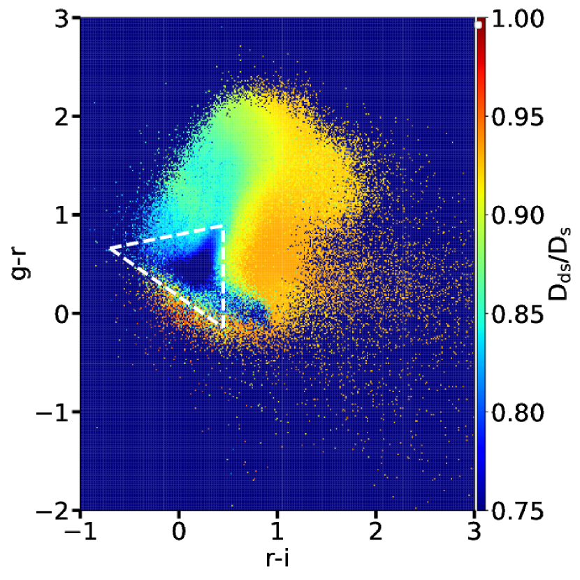
Figure 2: Ratio $D_{\mathrm{ds}}/D_{\mathrm{s}}$ of the distances between the observer and the sources and the lens and the sources in the colour-colour diagram. The horizontal axis shows r-i. The vertical axis shows g-r. Colour indicates the mean value of $D_{\mathrm{ds}}/D_{\mathrm{s}}$ in each pixel. The galaxies inside the triangle region are defined as the foreground and cluster member galaxies.

Figure 3: Redshift distribution of the source galaxies. The horizontal axis shows the redshift. The vertical axis shows the number count. We only used galaxies whose $i$-band magnitudes are between 21.5 and 24.5. The dotted line shows its distribution before adopting the selection criteria for the background galaxy. The solid line shows the result after adopting the criteria. The weighted mean redshift is 0.81.

We estimated $q^{*}_{\alpha}(\mbox{\boldmath$\theta$})$ at each galaxy position, $\theta$, by using as a fitting function second-order bi-polynomials of the vector $\theta$ with iterative $\sigma$-clipping rejection. Since the PSF distortion pattern in the VST data is locally variable, we carried out star and galaxy separation in each rectangular block. We then calibrated the KSB isotropic correction factor for individual objects using a subset of galaxies detected with high significance $\nu>50$. The isotropic PSF calibration was also carried out in the individual blocks used for the anisotropic PSF correction. We checked the ellipticities for galaxies detected over different pointings and found a general agreements. We then adopted the average of the ellipticity for the weak lensing mass measurement with the weight of equation (12).

The redshift of each galaxy in the $gri$ ShaSS photometric catalogues was estimated by using the COSMOS photometric redshift catalogue (Ilbert et al., 2013). We first computed the lensing kernel, $\beta_{i}\equiv{D_{\mathrm{ds},i}}/{D_{\mathrm{s},i}}$, of the $i-$th galaxy as an ensemble average of the $N$ nearest neighbours in the $gri-$ magnitude space of the $j$-th galaxy in the COSMOS catalogue,

$$\beta_{i}=\langle{D_{\mathrm{ds}}}/{D_{\mathrm{s}}}\rangle_{\rm COSMOS}=\frac{1}{N}\sum_{j}^{N}{D_{\mathrm{ds},j}}({z_{\mathrm{s}}})/{D_{\mathrm{s},j}}({z_{\mathrm{s}}}).$$ (20)

We then assigned the redshift of each galaxy from $\beta_{i}$, where we adopted $N=50$.

To define the foreground and background galaxies, we used the distance ratio in the colour-colour diagram. Fig. 2 shows the mean distance ratio in the colour-colour diagram. In the map, we divided the diagram into cells and calculated the mean value in each pixel. As seen in Fig. 2, there is a clump having the low value which corresponds to the cluster members and foreground galaxies. In order to exclude such galaxies, we defined the region residing in the clump as

$$g-r < 0.2(r-i)+0.8~{}({\rm for}~{}-0.4\leq r-i\leq 0.3),$$ (21)

$$g-r > -0.7(r-i)+0.17~{}({\rm for}~{}-0.4\leq r-i\leq 0.3),$$ (22)

$$r-i < 0.45~{}({\rm for}~{}0.17\leq g-r\leq 0.63).$$ (23)

To exclude the effects from bright stars on the shape measurement of the galaxies, we did not use galaxies which were closer than one star half-light radius from the brightest (<18 mag) stars. Moreover, we only used the galaxies between $r=21.5$ and $r=24.5$ magnitude. We could not find large dependence of shear profiles on the selection criteria and the magnitude of the bright stars. After adopting these cuts, the number density of galaxies for the shear measurement becomes $n_{g}=7$ arcmin^-2. Fig. 3 shows the redshift distribution for galaxies between $i=21.5-24.5$ magnitude before (dotted line) and after adopting the selection criteria (solid line). We can see that galaxies at lower redshifts are eliminated by adopting the colour cut. As a result, the mean source redshift weighted by the estimated errors of $D_{\rm ds}/D_{\rm s}$ becomes $z_{s}=0.81$ after the colour cut.

5 Results

5.1 Weak lensing mass reconstruction

We reconstructed the projected mass distribution, the so-called mass map, by following Kaiser & Squires (1993); Okabe & Umetsu (2008). We employed a Gaussian smoothing scale of FWHM$=10$ arcmin. Fig. 4 shows the WL mass map (contours) of the Shapely supercluster region for $r$ and $g-$bands, respectively. The errors were estimated by a bootstrap realization ($N=10000$) which randomly rotates galaxy orientations with fixed positions. The colours in the figures showed the galaxy number density derived from Haines et al. (2018). The WL mass distribution is highly associated with the spatial distribution of Shapley supercluster member galaxies (see Fig. 4). In particular, we find significant peaks around A 3556, A 3558, SC 1327-312, SC 1329-313, A 3562, and A 3559 in both $r$- and $g$-band images. Less pronounced peaks are associated with A 3560 and A 3554 in the $g$-band images, where a marginal detection of A 3552 is also present. The lack of WL signal in $r$-band images for the cluster A 3560 can be explained with the peculiar distortion affecting the $r$-band images of this VST field. On the other hand AS 0724 seems to be detected only in the $r$-band images. We could not find instead a clear peak around AS 0726 neither in the $r$- nor the $g$-band images.

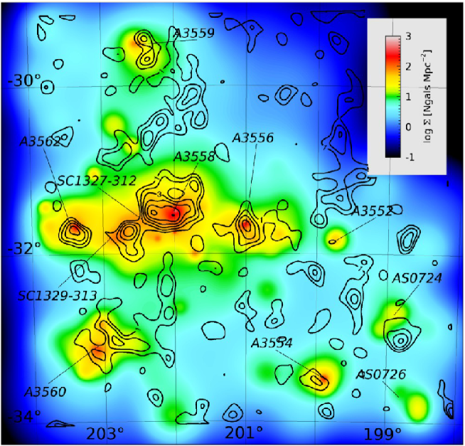
Figure 4: Galaxy number density from Haines et al. (2018) colour-coded as indicated in the right bar and with overlaid the contours of WL mass map as derived using the $r$-band imaging (upper panel) and $g$-band imaging (lower panel). The overlaid contours are stepped by $1\sigma$ from $1\sigma$.

Some of the mass peaks without any adjacent overdensity in supercluster galaxies are associated with background components (see Section 6). Therefore, our mass map is reasonably explained by the superposition of the supercluster component and background structures.

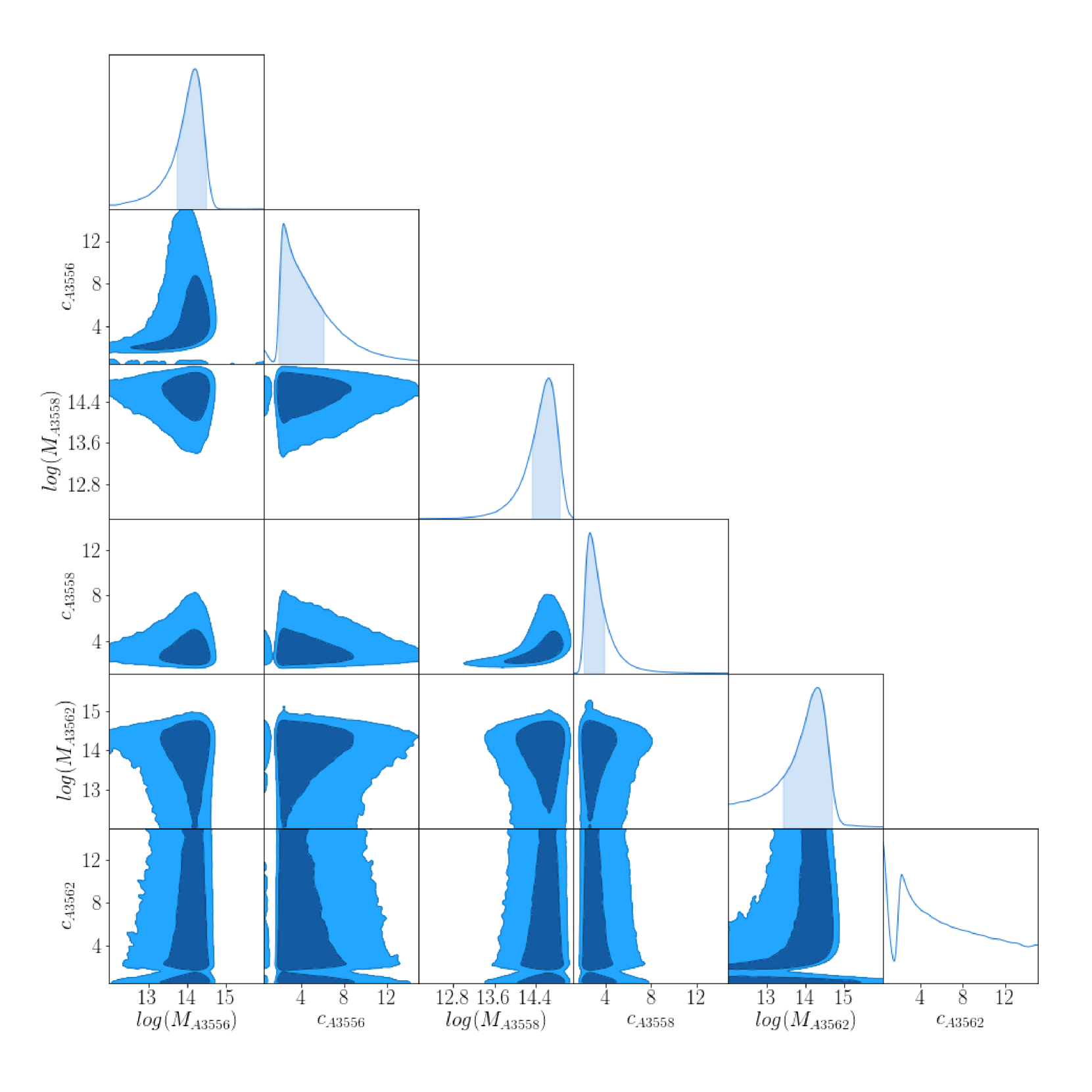
Figure 5: MCMC results for A 3556, A 3558 and A 3562 with a pixel scale of 3 arcmin. The horizontal axis shows mass $M_{200}$ in units of [$h^{-1}\mathrm{M}_{\odot}$]. The vertical axis shows concentration parameter. Contours are stepped by $1\sigma$.

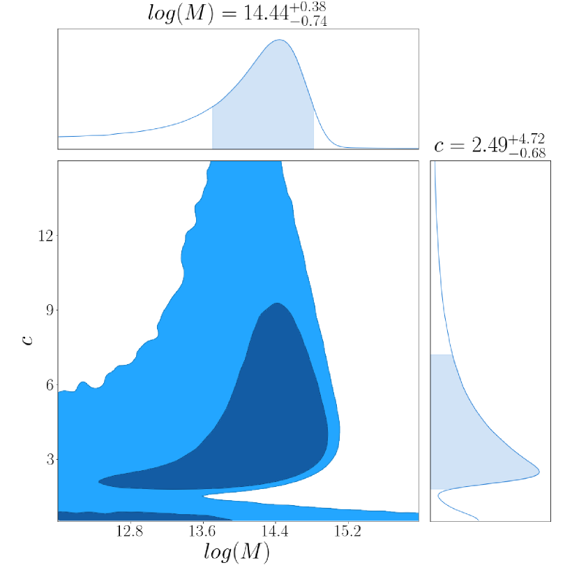
Figure 6: MCMC results for A 3560 with a pixel scale of 3 arcmin. The horizontal axis shows mass $M_{200}$ in units of [$h^{-1}\mathrm{M}_{\odot}$]. The vertical axis shows concentration parameter. Contours are stepped by $1\sigma$.

5.2 Fitting with the NFW profile

To estimate the mass and concentration parameters for each cluster, we fitted the shear values with the NFW profile on a two dimensional shear map. Due to the shape measurement problem, we could not derive the properties of the individual low mass clusters from the fitting. Therefore, the two-dimensional fitting was carried out only for the most massive clusters A 3556, A 3558, A 3560 and A 3562 (see Table 1). We simultaneously fitted the three clusters A 3556, A 3558 and A 3562 by assuming three NFW profiles. The cluster A 3560, which was far from the three clusters, was also fitted in the two-dimensional plane independently. On the other hand, we measured the tangential shear profiles for each low-mass cluster, and derived their mass and concentration parameters. Moreover, we stacked the shear profiles to investigate the average properties of the low-mass clusters.

In the two-dimensional fitting, we selected galaxies in the range of $200.3\leq\textrm{R.A.}\leq 203.8$ and $-32.1\leq\textrm{Dec.}\leq-31.1$ for the analysis of A 3556, A 3558 and A 3562. For A 3560, galaxies in the range of $202.6\leq\textrm{R.A.}\leq 203.6$ and $-33.6\leq\textrm{Dec.}\leq-32.6$ were instead used. The selected regions were divided into cells with the pixel scale of $3$ arcmin on a side. We calculated a shear value in each pixel by following equation (11). In the fitting, we used the positions of the brightest cluster galaxies (BCG) as the centres of the clusters. We ran the Markov chain Monte Carlo (MCMC) by parametrizing masses and concentration parameters. For analysis of the three clusters (A 3556, A 3558 and A 3562), we searched the best fitted parameters for each clusters simultaneously. In order to get the best fitted parameters from the chain distribution, we used the software ChainConsumer (Hinton, 2016). We also carried out the fitting for the cluster A 3560 independently.

In the calculation of the covariance matrix, we assumed that source galaxies are present at the average source redshift of the background galaxies. Since the ShaSS area is large, we only used the diagonal terms of the covariance matrix to reduce the computational time in the fitting. We searched the best fit parameters in the range $10^{13}M_{\odot}\leq M_{200}\leq 10^{16}M_{\odot}$ and $0.5\leq c\leq 15$. In order to check the effect of the pixel scale, we also ran the MCMC for the pixel scale of 2 arcmin and 4 arcmin, respectively. The obtained results were consistent with those for 3 arcmin within $2\sigma$. Moreover, we derived the masses for the $r-$band data. However, the obtained results are consistent with the masses estimated by $g$-band data within $2\sigma$. In addition, we also added the centres of the clusters as parameters for the fitting. We searched the centres within 5 armin from the positions from the BCGs. However, the offset between obtained centres and the positions of the BCGs were within a few arcmin while the centre for A 3560 did not converge. The differences for the other parameters were consistent within the error bar even in this case. Fig. 5 and 6 shows the MCMC results for A 3556, A 3558, and A 3562, and A 3560 respectively. Table 3 summarizes the results. For A 3562, the estimation for the concentration parameter did not converge, presumably because the off-centring between the position of the BCG and the weak lensing centre or large noises in galaxy shapes.

For the clusters with lower masses (AS 0724, A 3552, A 3554, A 3559, SC 1327-312 and SC 1329-313), we fitted their tangential shear profiles with the NFW profile in 11 annular bins from the BCG position out to 30 arcmin. In order to check the effects of the bin size on the obtained parameters, we increased and decreased the number of bins and fitted their profiles. We find that the results turn out to be consistent within the errors. The derived best-fit parameters are summarized in Table 4. Due to the low lensing signal, the fit does not converge for AS 0726. Fig. 7 shows the measured tangential and cross shear profiles with the best fitted NFW profile for each cluster.

For comparison and to investigate the average properties of the low-mass clusters, we also fitted the tangential shear profile obtained by stacking the shear profiles of the individual clusters weighted with the errors. In the stacking analysis, we included the profile of the cluster A 0726 and stacked the seven low mass clusters.

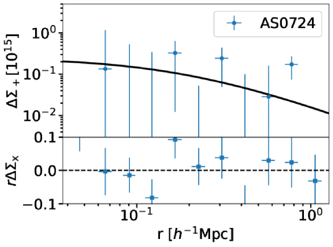
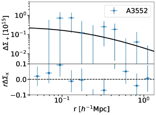
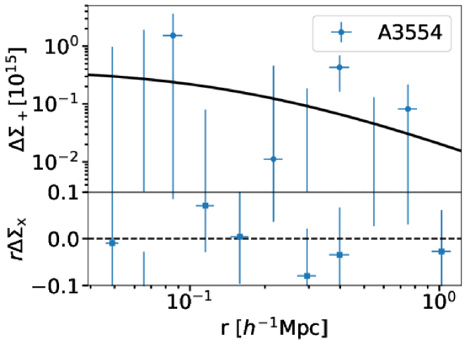
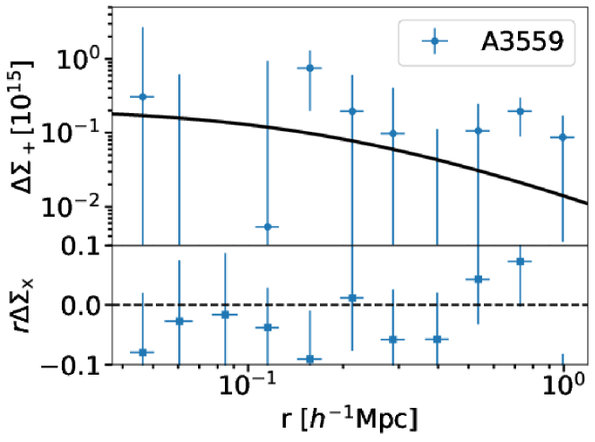
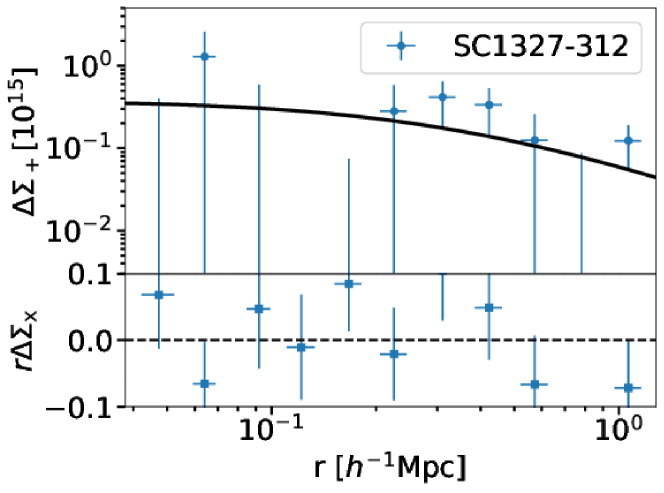
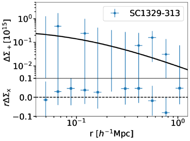
Figure 7: Tangential and cross shear profiles for the low mass clusters. The horizontal axis shows the distance from the BCG. The vertical axes for upper and lower panels show a tangential and cross shear profiles, respectively. The best-fitted NFW profiles are plotted as solid lines.

Fig. 8 shows the stacked shear profile with the best fitted profile. The estimated parameters are $M_{200}=(2.45^{+3.12})\times 10^{13}h^{-1}{\rm M}_{\odot}$ and $c=3.68^{+6.44}$. The large error is mainly caused by the small number of background galaxies.

Table 3: Fitting results of the massive clusters. The masses and concentration parameters are estimated by using the two-dimensional shear map with the pixel size of 3 arcmin. $1\sigma$ uncertainties are reported. Column (1): cluster name, Column (2): R.A. of BCG [degrees], Column (3): Dec. of BCG [degrees], Column (4): log($M_{200}[h^{-1}M_{\odot}]$), Column (5): concentration parameter.

	Cluster name	R.A.	Dec.	$M_{200}[10^{14}h^{-1}M_{\odot}]$	$c$
	A 3556	201.028071	-31.669883	$1.62^{+1.40}_{-1.08}$	$2.35^{+3.75}_{-0.47}$
	A 3558	201.986930	-31.495891	$4.47^{+2.78}_{-2.38}$	$2.63^{+1.23}_{-0.55}$
	A 3560	203.107375	-33.135833	$2.75^{+3.85}_{-2.25}$	$2.49^{+4.72}_{-0.68}$
	A 3562	203.394788	-31.672261	$2.04^{+2.74}_{-1.78}$

Table 4: Fitting results for the tangential shear profiles. Column (1): cluster name, Column (2): R.A. of BCG [degrees], Column (3): Dec. of BCG [degrees], Column (4): $M_{200}[h^{-1}M_{\odot}]$, Column (5): concentration parameter, Column (6): chi-square

Cluster name	R.A.	Dec.	$M_{200}[10^{13}h^{-1}M_{\odot}]$	$c$	$\chi^{2}/$d.o.f
AS 0724	198.247761	-33.0026810	$2.34^{+8.09}$	$3.90^{+18.84}$	9.18/9
A 3552	199.729591	-31.8175762	$3.01^{+17.22}$	$3.73^{+24.51}$	14.33/9
A 3554	199.881979	-33.4881320	$4.29^{+6.49}$	$5.67^{+2.34}$	5.97/9
A 3559	202.462143	-29.5143931	$1.79^{+14.92}$	$3.55^{+27.45}$	8.38/9
SC 1327-312	202.367236	-31.5512698	$4.31^{+49.25}$	$2.39^{+4.66}$	11.21/9
SC 1329-313	202.864741	-31.8206321	$1.79^{+2.93}$	$6.35^{+21.76}$	3.12/9

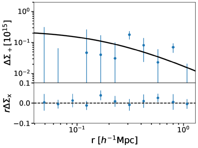
Figure 8: The stacked shear profile for the seven low mass clusters. The horizontal axis shows the distance from the BCGs. The upper and lower panels show the tangential and cross shear, respectively. The points show the results obtained from the observation. The solid line shows the best fitted result with the NFW profile.

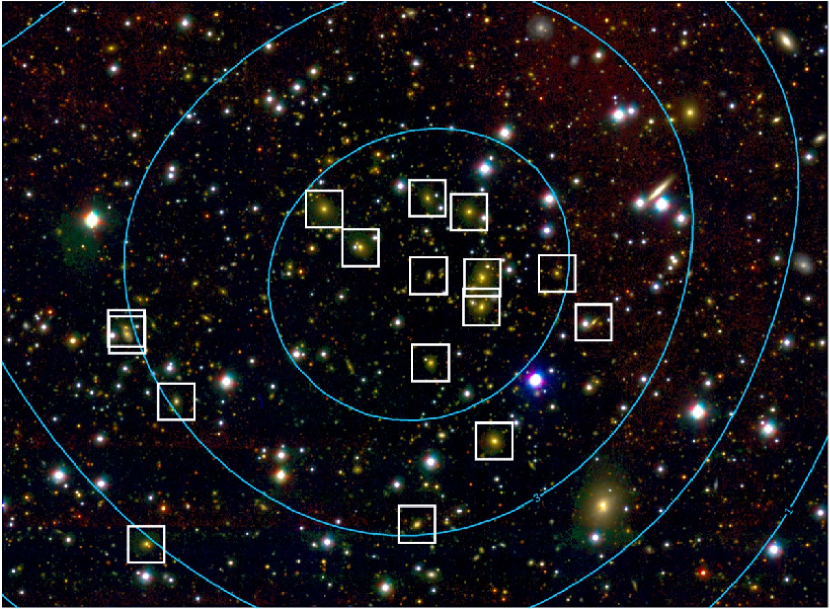
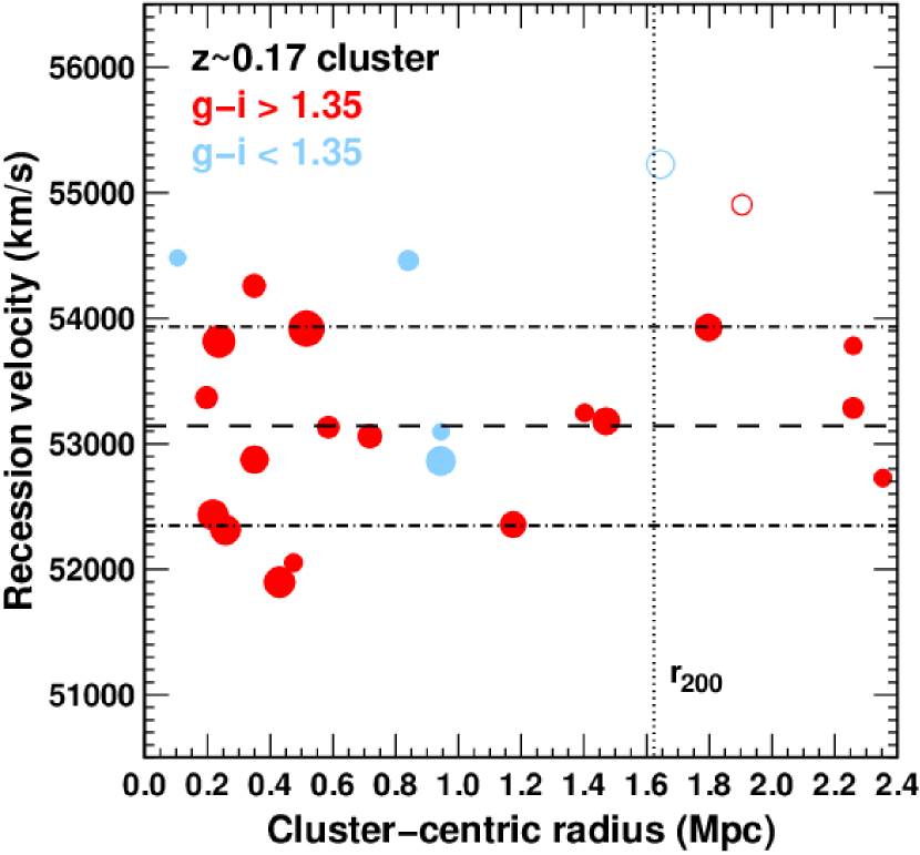
Figure 9: Upper panel: $gri$ colour composite image centred on the WL detection (blue contours) of a background cluster at redshift $z\sim 0.17$. The blue contours indicate the WL peak. Lower panel: Distribution of cluster members of the background cluster (solid dots, sizes scale with $i$-band luminosity) and non-members (open circles) in the caustic diagram; line-of-sight velocity,$cz$, versus projected distance from the centre of the WL peak. The dashed and dot-dashed lines indicate the central velocity and 1$\sigma$ velocity dispersion of member galaxies within $r_{200}$ (vertical dotted line).

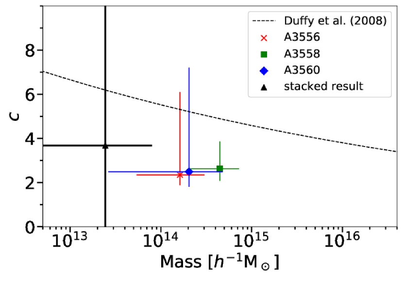
Figure 10: Comparison of $c-M$ relation between our result and the simulations of Duffy et al. (2008). The horizontal axis shows $M_{200}$. The vertical axis shows concentration parameter. The dashed line shows the simulation result. The error bars show $1\sigma$ uncertainties.

6 discussion

6.1 WL mass map revealing the supercluster and background structures

In Fig. 4 we showed the number density map of supercluster galaxies across the ShaSS as derived by Haines et al. (2018), superimposed with the contours of the WL mass maps obtained from the $r$- (upper panel) and $g$-band (lower panel) imaging. As already noted, both the WL maps show an overall agreement with the structure as traced by the galaxy number density, albeit with a few divergences due to either the different depths or distortions affecting certain fields. Both the WL maps well trace the supercluster core including the five clusters. In particular, the WL map obtained with $r$-band imaging shows a continuous structure between the five clusters at the $1\sigma$ level (upper panel in Fig. 4).

Merluzzi et al. (2015) and Haines et al. (2018) found a filament in the galaxy distribution which connects A 3559 to the centre of the supercluster. The density contrast of filaments being so low (Maturi & Merten, 2013; Higuchi et al., 2014), it is difficult to significantly detect such a structure in our analysis, however the WL contours have a trend to follow the filament connecting A 3559 to the supercluster core.

The WL mass maps also reveal a number of peaks that do not appear to be associated with any known cluster within the SSC. These peaks could instead be due to clusters located behind the SSC.

We take advantage of our extensive spectroscopic coverage of the entire ShaSS region to investigate the nature of these peaks. The $r$-band WL mass reconstruction shows a $\sim 4\sigma$ mass peak at RA=$202{\aas@@fstack{\circ}}1$, Dec=-$32{\aas@@fstack{\circ}}7$ that is not located near to any of the SSC clusters or any plausible grouping of SSC member galaxies. An examination of the redshifts of galaxies in the immediate vicinity of the WL peak reveals that the nine nearest galaxies ($d{<}160^{\prime\prime}$) all have $z\sim 0.177$, with a further nine $z\sim 0.177$ galaxies located within 8 arcmin. The $gri$ colour composite image of the region (Fig. 9) shows that the WL peak (blue contours) is centred on this dense concentration of red sequence galaxies, which are confirmed to lie within the redshift range $0.173<z<0.182$ (white squares). The lower panel shows the corresponding distribution of galaxies in the caustic diagram, plotting recession velocity ($V_{\mathrm{h}}$) versus projected distance from cluster centre (defined by the peak in the WL map), confirming that cluster membership is well-defined for this $z\sim 0.177$ system, with noticeable velocity gaps above 54 500 km s^-1 and below 51 700 km s^-1 where no galaxies are seen within 1.5 Mpc of the cluster centre. The biweight estimator (Beers et al., 1990) was used to derive a central recession velocity of 51 155 km s^-1 ($z=0.1773$) for the cluster and a velocity dispersion of $652{\pm}84$ km s^-1, based on 18 member galaxies within $r_{200}$ (1.62 Mpc), where $r_{200}$ was iteratively estimated from the $\sigma_{\nu}$ as in Haines et al. (2018). This implies a mass $M_{200}{=}5.7{\times}10^{14}{\rm M}_{\odot}$, comparable to that of Abell 3556.

The nature of the 5$\sigma$ mass peak located at RA=$198{\aas@@fstack{\circ}}8$, Dec=-$33{\aas@@fstack{\circ}}03$ is less clear. It is located 20^′ South of the nearest cluster AS 0724 within the Shapley supercluster, but also appears offset by 20^′ West from the extended structure at $z{\sim}0.10$ that runs up the Western boundary of the VST survey region (Chow-Martínez et al., 2014; Haines et al., 2018). The most likely correspondence appears to be with groups of galaxies at $z\sim 0.1$ to $z\sim 0.3$.

6.2 The $c-M$ relation of ShaSS massive clusters

Fig. 10 shows a comparison of the concentration parameters obtained from our fitting results and the $c-M$ relation derived by the simulations of Duffy et al. (2008). For the analytical model, the mean redshift of the clusters were adopted.

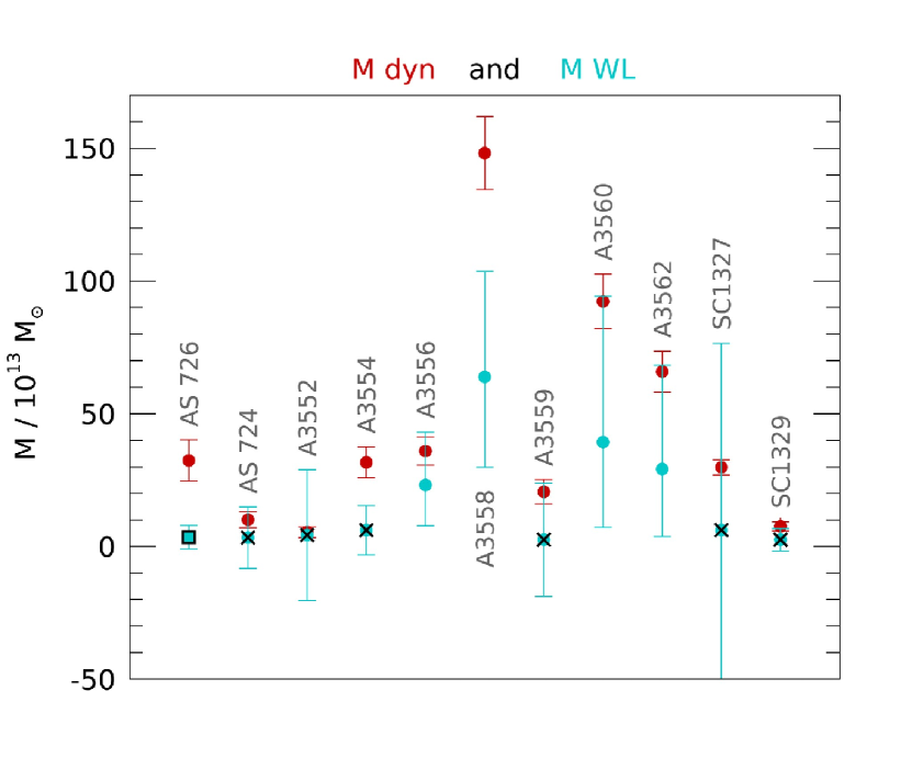
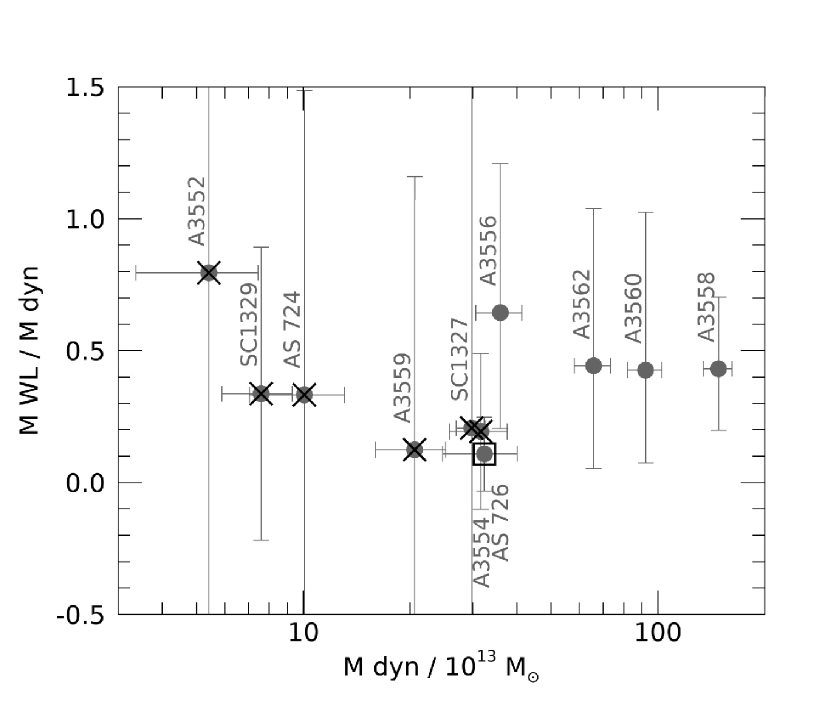
Figure 11: Left panel. The WL-derived masses (M_WL, cyan circles) for the 11 clusters are compared with the with the dynamical masses (M_dyn, red circles). Black crosses denote the low-mass clusters (see Table 1). Open black square denotes AS0726 for which the average mass for the low-mass clusters is adopted. Right panel. The ratio of WL-derived and dynamical masses as function of the dynamical mass for the 11 clusters. The 1$\sigma$ error bar is indicated in both panels.

Although our results turn out to be consistent with the simulations within $2\sigma$, the derived $c-M$ relations tend to be lower. While the results have large uncertainties, they could be explained by the dynamical state of the clusters. Previous studies showed that values of concentration parameters for unrelaxed clusters are lower than those for relaxed clusters of the same mass (Neto et al., 2007; Bhattacharya et al., 2013; Child et al., 2018; Okabe et al., 2019) and unrelaxed clusters having $\sim 30\%$ lower values of the concentration parameter in our mass range. Based on hierarchical structure formation, the high-overdensity environment of superclusters are more recently formed than normal clusters, so that the concentration of their components are expected to be lower. Therefore, the dynamical state or formation epoch of the constituent clusters could explain the smaller values of the concentration parameters in our results.

6.3 Cluster masses

In Fig. 11, we compared the WL-derived masses (M_WL) with those derived from the dynamical analysis(M_dyn) and listed in Table 1. The dynamical masses were computed under the assumption of the singular isothermal model and velocity dispersions (Haines et al., 2018). We obtained the WL masses for the four massive clusters (A 3556, A 3558, A 3560 and A 3562) with the MCMC method. On the other hand, we only gave the upper limit of the masses for 6 out of 7 low-mass clusters due to the large shape noise in the WL analysis. In the figure, we labeled the low-mass clusters as black crosses, AS 0726 as black box and the four massive clusters as cyan circles. For AS 0726, we only indicatively adopted the average mass for the low-mass clusters derived using the stacked shear profile. We notice that (i) the masses obtained from the dynamical and WL analysis are consistent within 1$\sigma$ for all clusters except A 3554, A 3558 and AS 0726; (ii) the dynamical masses turn out to be systematically higher than the WL- derived ones. Previous studies showed that WL masses obtained from the tangential shear fitting were biased low up to 10 percent with a scatter of $\sim 25$ percent (Oguri et al., 2005; Sereno & Umetsu, 2011; Sereno & Ettori, 2015). The main source of the bias are due to substructures and triaxiality. When a cluster whose major axis is perpendicular to the line of sight, i.e elongated in the sky-plane, a mass obtained with the spherical NFW profile is typically underestimated. The presence of substructures around clusters and uncorrelated large-scale structures along the line of sight also generate the biases for the estimation of the WL masses (Meneghetti et al., 2010; Becker & Kravtsov, 2011; Giocoli et al., 2012, 2014). In addtion, we point out that the dynamical mass of AS 0726 is actually an upper limit since the velocity distribution of member galaxies is strongly bimodal, and certainly not Gaussian (see Fig. 14 in Haines et al., 2018). This system probably consists of two groups with velocity dispersions $\sim 300$ km s^-1 rather than one single system with $\sigma\sim 600$ km s^-1. This would reduce the mass estimate by a factor 4. The complex structure of A 3558 and, in general, the dynamical activity in the SSC core (see Bardelli et al., 1998; Ettori et al., 2000; Finoguenov et al., 2004; Rossetti et al., 2007a) may explain the systematic differences between the two mass determinations quoted above, since the virial mass tends to overestimate the mass of unrelaxed clusters. Moreover, Rossetti et al. (2007b) studied A 3558 with a X-ray observation and showed the possibility of the presence of substructures along the line of sight, which interact with the cluster. Since such structures along the line of sight broaden velocity distribution, masses obtained from dynamical analysis can be overestimated up to 100% (Takizawa et al., 2010; Pratt et al., 2019). Fig. 14 in Haines et al. (2018) showed the broad velocity distribution of galaxies for the cluster. This indicates the presence of the substructures along the line of sight and the possibility for overestimating the dynamical mass. A 3554 also shows strong substructures in the velocity distribution diagram.

The WL and dynamical mass estimates for the massive clusters are actually consistent within 1$\sigma$ for three clusters and within 2$\sigma$ for A3558, even though we used different measurement techniques and different mass models. Thus, the total mass of the 4 massive clusters does not dramatically differ between the two approaches. We found their total masses $\mathcal{M}_{\rm 4cl,dyn}=(3.42\pm 0.20)\times 10^{15}{\rm M}_{\odot}$ and $\mathcal{M}_{\rm 4cl,WL}=(1.56^{+0.81}_{-0.55})\times 10^{15}{\rm M}_{\odot}$ - i.e. only a factor $\sim 2.2$ lower. By using the empirical L${}_{\rm X}-{\rm M}_{\rm 200}$ scaling relation of Böhringer, Hans et al. (2014) (their equation 10), we obtain $\mathcal{M}_{\rm 4cl,X}=(2.23\pm 0.7)\times 10^{15}{\rm M}_{\odot}$. The error of this estimates reflects the scatter of the mass–X-ray luminosity relation. While we could give upper limits of the masses for the low mass clusters, we got the total mass for the 11 clusters $\mathcal{M}_{\rm ShaSS,WL}=(1.84^{+1.13})\times 10^{15}{\rm M}_{\odot}$. In the calculation, we used the average mass derived from the stacking analysis for the mass of AS 0726. The total dynamical mass is $\mathcal{M}_{\rm ShaSS,dyn}=(4.80\pm 2.3)\times 10^{15}{\rm M}_{\odot}$.

Quintana et al. (1995) estimated a mass for the whole Shapley supercluster in the range $7\times 10^{15}-7\times 10^{16}{\rm M}_{\odot}$. Ragone et al. (2006) identified 122 galaxy systems across a $12\times 15$ degrees region centred in the SSC core and estimated their individual masses which summed up result in a total mass of $\mathcal{M}_{SSC}=6.88\times 10^{15}{\rm M}_{\odot}$. From the observed galaxy overdensity in a 285  deg² region, Proust et al. (2006) evaluated for the supercluster a total mass of $\mathcal{M}_{SSC}=7\times 10^{16}{\rm M}_{\odot}$. They also claimed that the result of Ragone et al. (2006) is a lower limit for the SSC mass.

All these mass estimates refered to the whole supercluster, on the other hand ShaSS covers 260 Mpc² centred on the core. Applying a spherical collapse model, Reisenegger et al. (2000) found that the SSC is gravitationally collapsing at least in its central region within a radius of 8 $h^{-1}$ Mpc, centred on A 3558 including 11 clusters; the very inner region, associated with the massive clusters, is likely in the final stages of collapse. The mass within this radius was found to be $\mathcal{M}_{\mathrm{SSC}}\sim 1.4\times 10^{16}{\rm M}_{\odot}$. On the other end, they same authors using the heuristic escape-velocity methods of Diaferio & Geller (1997) obtained a mass estimate of $\mathcal{M}_{\mathrm{SSC}}\sim 2.9\times 10^{15}{\rm M}_{\odot}$. This value is consistent within the errors with both our measurements of $\mathcal{M}_{\rm ShaSS,dyn}$ and $\mathcal{M}_{\rm ShaSS,WL}$.

7 Summary and conclusions

With the aim to investigate the mass distribution and thus to trace the environment in the centre of the Shapley supercluster (at $z\sim 0.048$), we have conducted the first weak lensing analysis of a 260 Mpc² region around the supercluster core including 11 clusters. This study has taken advantage of the multi-band ($gri$) optical imaging collected at ESO-VST together with the related photometric catalogues. These data have allowed us to generate the galaxy shape catalogues in $g$ and $r$ bands across the whole surveyed region. In the following the adopted approach is briefly described.

-

Supercluster members have been selected via photometric redshifts and background/foreground galaxies with the colour-colour diagram. The average density of the background galaxies turned out to be 7 arcmin^-2.

-

The project mass distributions, i.e. the WL mass maps have been derived for both $r$- and $g$-band data. The significance of the mass map has been estimated by randomizing the background galaxy shapes. The two maps allowed to double-check the final results especially in one fields affected by peculiar distortion.

-

Concentration parameters and masses were obtained fitting with the NFW profile the two-dimensional shear of the massive clusters (A 3556, A 3558, A 3560 and A 3562) and the tangential shear of the low-mass clusters (AS 0724, A 3552, A 3554, A 3559, SC 1327-312 and SC 1329-313). For the low mass clusters, we have also fitted their stacked tangential shear profile estimating their average mass and concentration parameter.

Our analysis of the ShaSS provides further evidence of the complex structure of the system and cluster-cluster interactions, reveals a new background cluster of galaxies, and provides WL-derived masses for the 11 clusters embedded in a common network.

-

We have found a tight correlation between WL mass distribution and the structure as traced by the galaxy density previously derived for the ShaSS. In particular, the WL map in $r$ band highlights that the SSC core consists of a coherent system and shows indications of a filaments connecting the SSC core and A 3559 in agreement with our previous study revealing a stream of galaxies in the same region.

-

The total WL-derived mass of the 4 massive clusters is $\mathcal{M}_{\mathrm{ShaSS,WL}}=(1.56^{+0.81}_{-0.55})\times 10^{15}{\rm M}_{\odot}$, which is consistent with their total dynamical mass. Adding the upper mass limits of the remaining clusters, the total mass is consistent with the total dynamical mass of Haines et al. (2018) and with Reisenegger et al. (2000) who analysed almost the same region of the ShaSS.

-

The WL-derived masses are found to be systematically lower than the dynamical ones for each cluster, although the different estimates are consistent within 1$\sigma$ for 8 out of 10 clusters. This discrepancy can be explained by the fact that in such a perturbed and dynamically-active environment, the cluster dynamical mass should be actually considered as an upper limit. In fact, the differences between the mass derivations are higher in the less relaxed and more substructured clusters. Likewise, the $c-M$ relation of ShaSS clusters shows concentration parameters typical of unrelaxed clusters.

-

Finally, in the WL mass map, we detect a peak associated to a previously unknown background cluster at $z\sim 0.177$ with a velocity dispersion of $652{\pm}84$ km s^-1 (based on 18 member galaxies within $r_{200}$=1.62 Mpc) and implying a mass $M_{200}{=}5.7{\times}10^{14}{\rm M}_{\odot}$, comparable to that of A 3556.

We conclude that the WL and dynamical analyses are complementary and both essential for a robust characterization of the supercluster environment allowing us to ascertain the continuity of the SSC structure around the core and supporting the scenario of an ongoing collapse.

References

- Bardelli et al. (1998) Bardelli S., Pisani A., Ramella M., Zucca E., Zamorani G., 1998, MNRAS, 300, 589
- Bardelli et al. (2000) Bardelli S., Zucca E., Zamorani G., Moscardini L., Scaramella R., 2000, MNRAS, 312, 540
- Bartelmann & Schneider (2001) Bartelmann M., Schneider P., 2001, Phys.~Rep., 340, 291
- Becker & Kravtsov (2011) Becker M. R., Kravtsov A. V., 2011, ApJ, 740, 25
- Beers et al. (1990) Beers T. C., Flynn K., Gebhardt K., 1990, AJ, 100, 32
- Bhattacharya et al. (2013) Bhattacharya S., Habib S., Heitmann K., Vikhlinin A., 2013, The Astrophysical Journal, 766, 32
- Böhringer, Hans et al. (2014) Böhringer, Hans Chon, Gayoung Collins, Chris A. 2014, A&A, 570, A31
- Bruzual & Charlot (2003) Bruzual G., Charlot S., 2003, MNRAS, 344, 1000
- Bullock et al. (2001) Bullock J. S., Kolatt T. S., Sigad Y., Somerville R. S., Kravtsov A. V., Klypin A. A., Primack J. R., Dekel A., 2001, MNRAS, 321, 559
- Capaccioli & Schipani (2011) Capaccioli M., Schipani P., 2011, The Messenger, 146, 2
- Cava et al. (2009) Cava A., et al., 2009, A&A, 495, 707
- Child et al. (2018) Child H. L., Habib S., Heitmann K., Frontiere N., Finkel H., Pope A., Morozov V., 2018, The Astrophysical Journal, 859, 55
- Chow-Martínez et al. (2014) Chow-Martínez M., Andernach H., Caretta C. A., Trejo-Alonso J. J., 2014, MNRAS, 445, 4073
- Courtois et al. (2017) Courtois H. M., Tully R. B., Hoffman Y., Pomarède D., Graziani R., Dupuy A., 2017, ApJ, 847, L6
- Diaferio & Geller (1997) Diaferio A., Geller M. J., 1997, The Astrophysical Journal, 481, 633
- Dietrich et al. (2012) Dietrich J. P., Werner N., Clowe D., Finoguenov A., Kitching T., Miller L., Simionescu A., 2012, Nature, 487, 202
- Drinkwater et al. (2004) Drinkwater M. J., Parker Q. A., Proust D., Slezak E., Quintana H., 2004, Publ. Astron. Soc. Australia, 21, 89
- Duffy et al. (2008) Duffy A. R., Schaye J., Kay S. T., Dalla Vecchia C., 2008, MNRAS, 390, L64
- Einasto et al. (2003) Einasto J., Hütsi G., Einasto M., Saar E., Tucker D. L., Müller V., Heinämäki P., Allam S. S., 2003, A&A, 405, 425
- Einasto et al. (2011) Einasto M., Liivamägi L. J., Tago E., Saar E., Tempel E., Einasto J., Martínez V. J., Heinämäki P., 2011, A&A, 532, A5
- Einasto et al. (2016) Einasto M., et al., 2016, A&A, 595, A70
- Einasto et al. (2018) Einasto M., et al., 2018, A&A, 620, A149
- Einasto et al. (2019) Einasto J., Suhhonenko I., Liivamägi L. J., Einasto M., 2019, A&A, 623, A97
- Ettori et al. (1997) Ettori S., Fabian A. C., White D. A., 1997, MNRAS, 289, 787
- Ettori et al. (2000) Ettori S., Bardelli S., de Grandi S., Molendi S., Zamorani G., Zucca E., 2000, Monthly Notices of the Royal Astronomical Society, 318, 239
- Finoguenov et al. (2004) Finoguenov A., Henriksen M. J., Briel U. G., de Plaa J., Kaastra J. S., 2004, The Astrophysical Journal, 611, 811
- Galametz et al. (2018) Galametz A., et al., 2018, MNRAS, 475, 4148
- Giacintucci et al. (2005) Giacintucci S., et al., 2005, A&A, 440, 867
- Giocoli et al. (2012) Giocoli C., Meneghetti M., Ettori S., Moscardini L., 2012, MNRAS, 426, 1558
- Giocoli et al. (2014) Giocoli C., Meneghetti M., Metcalf R. B., Ettori S., Moscardini L., 2014, MNRAS, 440, 1899
- Gonzalez et al. (2007) Gonzalez A. H., Zaritsky D., Zabludoff A. I., 2007, ApJ, 666, 147
- Gonzalez et al. (2013) Gonzalez A. H., Sivanandam S., Zabludoff A. I., Zaritsky D., 2013, ApJ, 778, 14
- Grado et al. (2012) Grado A., Capaccioli M., Limatola L., Getman F., 2012, Memorie della Societa Astronomica Italiana Supplementi, 19, 362
- Gray et al. (2009) Gray M. E., et al., 2009, MNRAS, 393, 1275
- Haines et al. (2018) Haines C. P., et al., 2018, MNRAS, 481, 1055
- Heymans et al. (2008) Heymans C., et al., 2008, MNRAS, 385, 1431
- Higuchi & Inoue (2019) Higuchi Y., Inoue K. T., 2019, MNRAS, 488, 5811
- Higuchi et al. (2014) Higuchi Y., Oguri M., Shirasaki M., 2014, MNRAS, 441, 745
- Hinton (2016) Hinton S. R., 2016, The Journal of Open Source Software, 1, 00045
- Ilbert et al. (2013) Ilbert O., et al., 2013, A&A, 556, A55
- Jee et al. (2014) Jee M. J., Hoekstra H., Mahdavi A., Babul A., 2014, ApJ, 783, 78
- Jing (2000) Jing Y. P., 2000, ApJ, 535, 30
- Jones et al. (2009) Jones D. H., et al., 2009, MNRAS, 399, 683
- Kaiser & Squires (1993) Kaiser N., Squires G., 1993, ApJ, 404, 441
- Kaiser et al. (1995) Kaiser N., Squires G., Broadhurst T., 1995, ApJ, 449, 460
- Kaldare et al. (2003) Kaldare R., Colless M., Raychaudhury S., Peterson B. A., 2003, MNRAS, 339, 652
- Kocevski et al. (2004) Kocevski D. D., Ebeling H., Mullis C. R., 2004, in Mulchaey J. S., Dressler A., Oemler A., eds, Clusters of Galaxies: Probes of Cosmological Structure and Galaxy Evolution. p. 26 (arXiv:astro-ph/0304453)
- Kron (1980) Kron R. G., 1980, ApJS, 43, 305
- Kuijken (2011) Kuijken K., 2011, The Messenger, 146, 8
- Kull & Böhringer (1999) Kull A., Böhringer H., 1999, A&A, 341, 23
- Lubin et al. (2009) Lubin L. M., Gal R. R., Lemaux B. C., Kocevski D. D., Squires G. K., 2009, AJ, 137, 4867
- Mahajan et al. (2018) Mahajan S., Singh A., Shobhana D., 2018, MNRAS, 478, 4336
- Maturi & Merten (2013) Maturi M., Merten J., 2013, A&A, 559, A112
- Medezinski et al. (2010) Medezinski E., Broadhurst T., Umetsu K., Oguri M., Rephaeli Y., Benítez N., 2010, MNRAS, 405, 257
- Mei et al. (2012) Mei S., et al., 2012, ApJ, 754, 141
- Meneghetti et al. (2010) Meneghetti M., Rasia E., Merten J., Bellagamba F., Ettori S., Mazzotta P., Dolag K., Marri S., 2010, A&A, 514, A93
- Mercurio et al. (2015) Mercurio A., et al., 2015, MNRAS, 453, 3685
- Merluzzi et al. (2015) Merluzzi P., et al., 2015, MNRAS, 446, 803
- Merluzzi et al. (2016) Merluzzi P., Busarello G., Dopita M. A., Haines C. P., Steinhauser D., Bourdin H., Mazzotta P., 2016, MNRAS, 460, 3345
- Miller (2005) Miller N. A., 2005, AJ, 130, 2541
- Muñoz & Loeb (2008) Muñoz J. A., Loeb A., 2008, MNRAS, 391, 1341
- Navarro et al. (1997) Navarro J. F., Frenk C. S., White S. D. M., 1997, ApJ, 490, 493
- Neto et al. (2007) Neto A. F., et al., 2007, Monthly Notices of the Royal Astronomical Society, 381, 1450
- Oguri et al. (2004) Oguri M., Takahashi K., Ichiki K., Ohno H., 2004, arXiv Astrophysics e-prints,
- Oguri et al. (2005) Oguri M., Takada M., Umetsu K., Broadhurst T., 2005, ApJ, 632, 841
- Oguri et al. (2010) Oguri M., Takada M., Okabe N., Smith G. P., 2010, MNRAS, 405, 2215
- Oguri et al. (2012) Oguri M., Bayliss M. B., Dahle H., Sharon K., Gladders M. D., Natarajan P., Hennawi J. F., Koester B. P., 2012, MNRAS, 420, 3213
- Okabe & Umetsu (2008) Okabe N., Umetsu K., 2008, PASJ, 60, 345
- Okabe et al. (2010) Okabe N., Takada M., Umetsu K., Futamase T., Smith G. P., 2010, PASJ, 62, 811
- Okabe et al. (2013) Okabe N., Smith G. P., Umetsu K., Takada M., Futamase T., 2013, ApJ, 769, L35
- Okabe et al. (2014) Okabe N., Futamase T., Kajisawa M., Kuroshima R., 2014, ApJ, 784, 90
- Okabe et al. (2016) Okabe N., et al., 2016, MNRAS, 456, 4475
- Okabe et al. (2019) Okabe N., et al., 2019, Publications of the Astronomical Society of Japan, 71, 79
- Planck Collaboration et al. (2014) Planck Collaboration et al., 2014, A&A, 571, A31
- Pratt et al. (2019) Pratt G. W., Arnaud M., Biviano A., Eckert D., Ettori S., Nagai D., Okabe N., Reiprich T. H., 2019, Space Sci. Rev., 215, 25
- Proust et al. (2006) Proust D., et al., 2006, A&A, 447, 133
- Quintana et al. (1995) Quintana H., Ramirez A., Melnick J., Raychaudhury S., Slezak E., 1995, AJ, 110, 463
- Quintana et al. (1997) Quintana H., Melnick J., Proust D., Infante L., 1997, A&AS, 125, 247
- Ragone et al. (2006) Ragone C. J., Muriel H., Proust D., Reisenegger A., Quintana H., 2006, A&A, 445, 819
- Raychaudhury (1989) Raychaudhury S., 1989, Nature, 342, 251
- Reisenegger et al. (2000) Reisenegger A., Quintana H., Carrasco E. R., Maze J., 2000, AJ, 120, 523
- Rossetti et al. (2007b) Rossetti M., Ghizzardi S., Molendi S., Finoguenov A., 2007b, A&A, 463, 839
- Rossetti et al. (2007a) Rossetti M., Ghizzardi S., Molendi S., Finoguenov A., 2007a, A&A, 463, 839
- Schlafly & Finkbeiner (2011) Schlafly E. F., Finkbeiner D. P., 2011, ApJ, 737, 103
- Sereno & Ettori (2015) Sereno M., Ettori S., 2015, MNRAS, 450, 3633
- Sereno & Umetsu (2011) Sereno M., Umetsu K., 2011, MNRAS, 416, 3187
- Takizawa et al. (2010) Takizawa M., Nagino R., Matsushita K., 2010, PASJ, 62, 951
- Tully (2005) Tully R. B., 2005, ApJ, 618, 214
- Umetsu et al. (2010) Umetsu K., Medezinski E., Broadhurst T., Zitrin A., Okabe N., Hsieh B.-C., Molnar S. M., 2010, ApJ, 714, 1470
- Umetsu et al. (2011) Umetsu K., Broadhurst T., Zitrin A., Medezinski E., Coe D., Postman M., 2011, ApJ, 738, 41
- Umetsu et al. (2014) Umetsu K., et al., 2014, ApJ, 795, 163
- Umetsu et al. (2016) Umetsu K., Zitrin A., Gruen D., Merten J., Donahue M., Postman M., 2016, ApJ, 821, 116
- Venturi et al. (2003) Venturi T., Bardelli S., Dallacasa D., Brunetti G., Giacintucci S., Hunstead R. W., Morganti R., 2003, A&A, 402, 913
- Wright & Brainerd (2000) Wright C. O., Brainerd T. G., 2000, ApJ, 534, 34
- Yaryura et al. (2011) Yaryura C. Y., Baugh C. M., Angulo R. E., 2011, MNRAS, 413, 1311
- York et al. (2000) York D. G., et al., 2000, AJ, 120, 1579
- Zhao et al. (2009) Zhao D. H., Jing Y. P., Mo H. J., Börner G., 2009, ApJ, 707, 354
- de Filippis et al. (2005) de Filippis E., Schindler S., Erben T., 2005, A&A, 444, 387