Learning Expected Reward for Switched Linear Control Systems: A Non-Asymptotic View

Abstract

In this work, we show existence of invariant ergodic measure for switched linear dynamical systems (SLDSs) under a norm-stability assumption of system dynamics in some unbounded subset of $\mathbb{R}^{n}$. Consequently, given a stationary Markov control policy, we derive non-asymptotic bounds for learning expected reward (w.r.t the invariant ergodic measure our closed-loop system mixes to) from time-averages using Birkhoff’s Ergodic Theorem. The presented results provide a foundation for deriving non-asymptotic analysis for average reward-based optimal control of SLDSs. Finally, we illustrate the presented theoretical results in two case-studies.

1 Introduction

Last decade has seen tremendous advancements in non-asymptotic analysis of system identification and optimal control for linear time-invariant dynamical systems (e.g., Tu und Recht (2018); Hao u. a. (2020); Oymak (2019); Fazel u. a. (2018); Simchowitz u. a. (2018); Sarkar u. a. (2019)). When evaluating a value function corresponding to a policy for the infinite-horizon case, existing literature in non-asymptotic analysis, such as Lazaric u. a. (2012); Tu und Recht (2018), uses a discount factor on instantaneous rewards; this results in a policy iteration algorithm that computes a new policy that minimize immediate rewards rather than minimizing the cumulative reward over infinite horizon. While this approach might be valid for some application domains (e.g., finance), it may not be suitable in general setting; in the general case, it is preferable to minimize the expected reward with respect to the stationary distribution induced by the choice of the control policy Bertsekas (1995).

The main challenge in using this approach is that, when system dynamics is not known, we do not have access to the stationary distribution. However, let us assume that we do have access to instantaneous rewards and are able to show that the underlying dynamical system mixes geometrically to an invariant ergodic measure. Then, the expected reward w.r.t the stationary distribution induced by our choice of control policy can be approximated from time-averages of instantaneous rewards, under mild assumptions on the reward function. On the other hand, when system dynamics is unknown, average reward-based optimal control requires bounds on the mixing time; i.e, these methods require a bound on the length of time-averages of the reward that, with high probability, approximate the expected reward w.r.t the stationary distribution induced by the choice of the control policy. Zahavy u. a. (2019) recently provided non-asymptotic analysis for this problem when the underlying state-space is discrete. In this work, we focus on the case when the controlled dynamical systems is an unknown switched linear dynamical system in continuous state-space $\mathbb{R}^{n}$. We first show sufficient conditions for existence of an ergodic invariant distribution. After establishing existence, we provide analysis for non-asymptotic sample complexity of learning the expected reward from its time-averages.

1.1 Preliminaries and Background

Notation.

$\mathbb{N}$ and $\mathbb{R}$ denote the sets of natural and real numbers, respectively. ${I}_{n}\in\mathbb{R}^{n\times n}$ denotes the $n$ dimensional identity matrix, whereas $\|\nu-\mu\|_{tv}$ is the total variation distance between probability measures $\mu$ and $\nu$. For random variables $x$ and $y$, $\mathbb{E}(x)$ and $Cov(x,y)$ denote the expectation and covariance. $\lambda^{n}()$ is the n-dimensional Lebesgue measure, and $\mathbb{B}_{\mathbb{R}^{n}}$ is Borel $\sigma$-algebra on $\mathbb{R}^{n}$. $\mathcal{B}_{\alpha}^{n}:=\{x\in\mathbb{R}^{n}:\|x\|_{2}\leq\alpha\}$ is the $\alpha$-ball in $\mathbb{R}^{n}$. Also, $y_{n}\xrightarrow{a.s}y$ denotes that $y_{n}$ converges almost surely to $y$, whereas to simplify our presentation $a\land b$ denotes $\min(a,b)$. $\chi_{\{\}}()$ is the indicator function, $Q\succ 0$ ($Q\succeq 0$) denotes that matrix $Q$ is positive (semi)definite, and $\rho(A)$ is the spectral radius of matrix $A\in\mathbb{R}^{n\times n}$. Finally, for a set $\mathcal{K}\subseteq\{1,...,M\}$, its complement is $\mathcal{K}^{\complement}:=\{1,...,M\}\setminus\mathcal{K}$.

Background.

We consider a discrete-time switched linear dynamical system (SLDS) of the form

$$x_{t+1}=\sum_{j=1}^{M}(A_{j}x_{t}+B_{J}u_{t}+w_{t}^{j})\chi_{\mathcal{M}_{j}}(x_{t}).$$ (1)

Here, $x_{t}\in\mathbb{R}^{n},u_{t}\in\mathbb{R}^{p}$ denote the system’s state and input, respectively, and $A_{j}\in\mathbb{R}^{n\times n}$ and $B_{j}\in\mathbb{R}^{n\times p}$, $j=1,...,M$, capture system dynamics in each of the $M$ regions that decompose the state-space – the regions, defined as $\mathcal{M}_{j}=\{x\in\mathbb{R}^{n}:L_{j}x\leq C_{j}\}$, $j=1,...,M$, are pairwise disjoint satisfying $\bigcup_{j=1}^{M}\mathcal{M}_{j}=\mathbb{R}^{n}$. In addition, for a fixed region $j$, noise vectors $w_{t}^{j}$ are i.i.d, and satisfy $w_{t}^{j}\thicksim\mathcal{N}(0,{I}_{n})$ and $Cov(w_{t}^{j},w_{s}^{k})=0$, for all $t,s\geq 0$ and $j\neq k\in\{1,2,...,M\}$.

We assume that the applied control law $u_{t}$ is a linear function of state $x_{t}$ weighted by policy $\pi$ – i.e., $u_{t}=\pi x_{t}$, with $\pi\in\mathbb{R}^{p\times n}$. We use a common (control) reward function $r(x,u)=\sqrt{x^{T}Qx+u^{T}Ru}$, where $Q\succcurlyeq 0,R\succ 0$, and $Q,R\in\mathbb{R}^{n\times n}$ Bertsekas (1995). Hence, under the control law $u=\pi x$, which we also denote as $u=\pi(x)$, we have that $r(x,\pi x)=\sqrt{x^{T}(Q+\pi^{T}R\pi)x}$; furthermore, the closed-loop dynamics of (1) can be captured as

$$x_{t+1}=\sum_{j=1}^{M}\big{(}\underbrace{(A_{j}+B_{J}\pi)}_{\hat{A}_{j}^{\pi}}x_{t}+w_{t}^{j}\big{)}\chi_{\mathcal{M}_{j}}(x_{t})=\sum_{j=1}^{M}\left(\hat{A}_{j}^{\pi}x_{t}+w_{t}^{j}\right)\chi_{\mathcal{M}_{j}}(x_{t}).$$ (2)

Finally, if $x_{t}$ from (2) under policy $\pi$ mixes to a stationary distribution $\nu_{\pi}$, we define the steady-state reward $\rho(\pi)$ associated with the policy $\pi$ as $\rho(\pi)=\mathbb{E}_{x\thicksim\nu_{\pi}}r(x,\pi(x))$.

The contributions of this paper are twofold. First, we derive sufficient conditions under which samples of the closed-loop system trajectories from (2), under policy $\pi$, mix geometrically to a unique ergodic invariant measure $\nu_{\pi}$ (in Section 2). Second, when the closed-loop system in (2) satisfies the derived conditions, leveraging Birkhoff’s pointwise ergodic theorem, which implies

$$\lim_{N\rightarrow\infty}\frac{1}{N}\sum\nolimits_{t=0}^{N-1}r(x_{t},\pi(x_{t}))\xrightarrow{a.s}\int r(y,\pi(y))\nu_{\pi}(dy)=:\rho(\pi),$$ (3)

we provide finite sample analysis for learning $\rho(\pi)$, defined in (3), with high probability from time averages $\frac{1}{N}\sum_{t=0}^{N-1}r(x_{t},\pi(x_{t}))$ (in Section 3). We show that the complexity of the sample analysis linearly depends on the size of the state space as opposed to quadratic dependence when a discounted LQR is used on commonly considered linear Gaussian dynamical systems (e.g., as in Tu und Recht (2018)). Finally, we validate the presented results on case studies (in Section 4).

2 Mixing of SLDSs to Invariant Distributions

We start by considering a linear time-invariant dynamical system with a state-space representation

$$x_{t+1}=Ax_{t}+w_{t},$$ (4)

where $(w_{t})_{t\in\mathbb{N}}$ is i.i.d with distribution $\mathcal{N}(0,{I}_{n})$ and spectral radius $\rho(A)$ satisfies that $\rho(A)<1$. For $\mathcal{A}\in\mathbb{B}_{\mathbb{R}^{n}}$ and any $s\in\mathbb{N}$, one step transition kernel is defined as $P(x,\mathcal{A})=\mathbb{P}(x_{s+1}\in\mathcal{A}|x_{s}=x)$ and $k^{\text{th}}$ step transition kernel is denoted by $P^{k}(x,\mathcal{A})=\mathbb{P}(x_{s+k}\in\mathcal{A}|x_{s}=x)$. Proving existence of an ergodic invariant measure using a total variation approach, would require showing that for all $x,y\in\mathbb{R}^{n}$ it holds that $\lim_{t\rightarrow\infty}\|P^{t}(x,\cdot)-P^{t}(y,\cdot)\|_{tv}=0$.

For SLDS (4), $P(x,\cdot)=\mathcal{N}(Ax,I_{n})$, and it is a common knowledge that the sequence from (4) mixes geometrically to a unique ergodic invariant Gaussian distribution Tu und Recht (2018); at the same time $\sup_{(x,y)\in\mathbb{R}^{n}\times\mathbb{R}^{n}}\|P(x,\cdot)-P(y,\cdot)\|_{tv}=2$, making total variation approach infeasible for Gaussian kernel on unbounded state space. Adding to the difficulty of SLDS analysis, the transition kernel for the state sequence of the closed-loop system (2) is more complex than for linear time-invariant systems (4), which is a standard benchmark in non-asymptotic analysis(e.g., Abbasi-Yadkori u. a. (2019); Tu und Recht (2018)).

This brings us to the theory of Wasserstein metric and optimal transport Villani (2008), which is used to construct a metric on $\mathcal{P}(\mathbb{R}^{n})\times\mathcal{P}(\mathbb{R}^{n})$ under which (2) mixes to an invariant measure; here, $\mathcal{P}(\mathbb{R}^{n})$ is the space of probability measures on $\mathbb{R}^{n}$. For a lower semi-continuous metric $d(x,y)$ on $\mathbb{R}^{n}\times\mathbb{R}^{n}$, Wasserstein metric on $\mathcal{P}(\mathbb{R}^{n})$ is defined as

$$\mathcal{W}_{d}^{1}(\nu,\mu)=\inf_{(X,Y)\in\Gamma(\nu,\mu)}\mathbb{E}~{}d(X,Y);$$ (5)

here, $(\nu,\mu)\in\mathcal{P}(\mathbb{R}^{n})\times\mathcal{P}(\mathbb{R}^{n})$, and $(X,Y)\in\Gamma(\nu,\mu)$ implies that random variables $(X,Y)$ follow probability distributions on $\mathbb{R}^{n}\times\mathbb{R}^{n}$ with marginals $\nu$ and $\mu$. For example, if $d(x,y):=\chi_{x\neq y}(x,y)$, it follows that

$$\mathcal{W}^{1}(\nu,\mu)=\inf_{(X,Y)\in\Gamma(\nu,\mu)}\mathbb{P}(X\neq Y)=\frac{1}{2}\|\nu-\mu\|_{tv}.$$ (6)

For any function $V:\mathbb{R}^{n}\rightarrow[0,\infty)$, we define $\mathcal{P}V(x):=\int_{\mathbb{R}^{n}}V(y)P(x,dy)$. Intuitively speaking, to prove existence of an invariant measure, our goal is to show that for all $x,y\in\mathbb{R}^{n}$ their exists some metric $d_{\mathcal{P}}$ on $\mathcal{P}(\mathbb{R}^{n})\times\mathcal{P}(\mathbb{R}^{n})$ such that $d_{\mathcal{P}}$ acts as a contraction on the transition kernel of (2) – i.e.,

$$d_{\mathcal{P}}\left(P^{t}(x,\cdot),P^{t}(y,\cdot)\right)\leq\eta\cdot d_{\mathcal{P}}\left(P^{t-1}(x,\cdot),P^{t-1}(y,\cdot)\right),$$ (7)

for some $\eta<1$ and all $t\in\mathbb{N}$. If the space $\mathcal{P}(\mathbb{R}^{n})$ is complete under the metric $d_{\mathcal{P}}$, (7) implies existence of a unique invariant measure that the SLDS from (2) mixes to. Hairer (2010) introduces corresponding easy-to-verify conditions; if there exist function $V(x),\gamma\in(0,1),K\in\mathbb{R}$, and $\alpha>0$ s.t.

$$(i) \hskip 10.0pt\mathcal{P}V(x)\leq\gamma V(x)+K,~{}\hskip 50.0pt\text{for all }~{}x\in\mathbb{R}^{n}$$ (8)

$$(ii) \hskip 10.0pt\|P(x,\cdot)-P(y,\cdot)\|_{tv}\leq 2(1-\alpha),\hskip 8.0pt\text{for all }~{}{(x,y)\in\mathbb{R}^{n}\times\mathbb{R}^{n}~{}s.t.~{}V(x)+V(y)\leq\hat{r}},$$ (9)

with $\hat{r}>\frac{2K}{1-\gamma}$, then system (2) mixes geometrically to a unique ergodic invariant measure.

In the above condition, (8) ensures that the dynamical system is being ‘pushed’ to a neighborhood of the origin in $\mathbb{R}^{n}$. (9) implies existence of a sufficiently large level set such that any two trajectories, with distinct initial conditions inside the level set, can be ‘coupled’ together with positive probability; i.e., if $X\thicksim P(x,\cdot)$ and $Y\thicksim P(y,\cdot)$ for $x,y$ in the aforementioned sufficiently large level set, then $\mathbb{P}(X\neq Y)\leq(1-\alpha)$ (see Kulik (2015) for more details) and $\mathbb{P}(X_{n}\neq Y_{n})\leq(1-\alpha)^{n}$. This implies that distinct trajectories overlap with positive probability and it becomes more and more unlikely as $n$ increases that they diverge away from each other. As shown in Hairer (2010); Eberle (2015) , (8) and (9) ensure existence of a probability metric which acts as a contraction on the transition kernel, i.e.,  (7) holds for $d_{\mathcal{P}}:=\mathcal{W}_{d_{{\beta}^{\ast}}}^{1}$, as defined in (5), where $d_{\beta^{\ast}}(x,y):=(2+\beta^{\ast}V(x)+\beta^{\ast}V(y))\cdot\chi_{x\neq y}(x,y)$ for some $\beta^{\ast}>0$ and $\eta<1$; note here that $\eta$ depends on $\alpha$ and $\beta^{\ast}$. Furthermore, completeness of $\mathcal{P}(\mathbb{R}^{n})$ equipped with metric $\mathcal{W}_{d_{\beta^{\ast}}}^{1}$ directly follows from lower semi-continuity of $d_{\beta^{\ast}}(x,y)$.

Theorem 1.

Consider a control law $u_{t}=\pi(x_{t})$, and assume that there exists $\varrho<\infty$ such that for all $k_{\text{unbdd}}\in\mathcal{K}_{unbdd}:=\left\{k~{}|~{}(1\leq k\leq M)\text{ and }\left((\mathcal{M}_{k}\cap(\mathcal{B}^{n}_{\varrho})^{\complement})\neq\emptyset\right)\right\}$, it holds that $\|\hat{A}_{k_{\text{unbdd}}}^{\pi}\|_{2}<1$. Then, the system (2) mixes geometrically to a unique ergodic invariant distribution $\nu_{\pi}$.

Before proving Theorem 1, note that the theorem assumption is that, given a control law $u_{t}=\pi(x_{t})$ there exists a bounded ball around the origin where the closed-loop dynamics might be unstable, but is stable outside the ball. The bounded set is essentially same as the aforementioned ‘sufficiently large level set’, and to show that (8) and (9) hold, we proceed as follows.

Proof.

Consider function $V(x)=\|x\|_{2}^{2}$. From (2), we have $P(x,\mathcal{A})=\sum_{j=1}^{M}P_{j}(x,\mathcal{A})\chi_{\mathcal{M}_{j}}(x)$, where $P_{j}(x,\cdot)\thicksim\mathcal{N}(\hat{A}_{j}^{\pi}x,{I}_{n})$. We define $c:=\max_{k\in\mathcal{K}_{unbdd}^{\complement}}\|\hat{A}_{k}^{\pi}\|_{2}^{2}$ and $\gamma:=\max_{j\in\mathcal{K}_{unbdd}}\|\hat{A}_{j}^{\pi}\|_{2}^{2}$; then, from the theorem assumption it holds that $\gamma<1$.

If we assume that the initial state $x_{0}:=x$ satisfies $\|x\|_{2}\leq\varrho$, then there exists a $k\in\mathcal{K}_{unbdd}^{\complement}$ such that

$$\mathcal{P}V(x)=\mathbb{E}_{y\thicksim\mathcal{N}(\hat{A}_{k}^{\pi}x,I_{n})}\|y\|_{2}^{2}=\mathbb{E}_{z\thicksim\mathcal{N}(0,I_{n})}\|z\|_{2}^{2}+\|\hat{A}_{k}^{\pi}x\|_{2}^{2}\leq(n+c\varrho^{2}).$$ (10)

However, if the initial state is $x_{0}:=x$ such that $\|x\|_{2}>\varrho$, then there exists $j\in\mathcal{K}_{unbdd}$ such that

$$\mathcal{P}V(x)=\mathbb{E}_{y\thicksim\mathcal{N}(\hat{A}_{j}^{\pi}x,I_{n})}\|y\|_{2}^{2}=\mathbb{E}_{z\thicksim\mathcal{N}(0,I_{n})}\|z\|_{2}^{2}+\|\hat{A}_{j}^{\pi}x\|_{2}^{2}\leq n+\gamma\|x\|_{2}^{2}=(n+\gamma V(x)).$$ (11)

Therefore, starting from any initial condition in $\mathbb{R}^{n}$, from (10) and (11) it holds that

$$\mathcal{P}V(x)\leq\gamma V(x)+\underbrace{(n+c\varrho^{2})}_{K},$$ (12)

and thus (8) holds for the closed-loop dynamical system from (2) under the theorem assumptions.

To show (9), we define

$$\hat{r}:=\frac{2(n+c\varrho^{2})}{\gamma(1-\gamma)}\qquad\Rightarrow\qquad\hat{r}>\frac{2(n+c\varrho^{2})}{(1-\gamma)},$$ (13)

where the right side holds since $\gamma<1$. For any $x,y\in\mathbb{R}^{n}$, $P(x,\cdot)$ and $P(y,\cdot)$ follow $\mathcal{N}(\hat{A}_{j}^{\pi}x,{I}_{n})$ and $\mathcal{N}(\hat{A}_{k}^{\pi}y,{I}_{n})$ respectively, for some $j,k\in\{1,2,..,M\}$. Gaussians are absolutely continuous w.r.t. Lebesgue measure, implying that $\|P(x,\cdot)-P(y,\cdot)\|_{tv}=2-2\int_{\mathbb{R}^{n}}(f_{x}(z)\land g_{y}(z))dz$ (see e.g., van Handel (2014)), with $f_{x}(z)$ and $g_{y}(z)$ being the density functions of $P(x,\cdot)$ and $P(y,\cdot)$, respectively. Now, let us define

$$\alpha_{(x,y)}:=\int_{\mathbb{R}^{n}}(f_{x}(z)\land g_{y}(z))dz$$

We have that $\alpha_{(x,y)}=0\iff f_{x}(z)\land g_{y}(z)=0$ almost everywhere (a.e.) w.r.t. Lebesgue measure on $\mathbb{R}^{n}$ Folland (2013). Thus, the existence of $\alpha_{(x,y)}>0$, for any specific $(x,y)$, directly follows if we can show that $f_{x}(z)\land g_{y}(z)>0$ a.e. w.r.t. Lebesgue measure on $\mathbb{R}^{n}$. We show in Appendix under the heading of Claim 1, that for each $(\hat{x},\hat{y})\in\mathcal{D}$, where $\mathcal{D}:=\{(x,y)\in\mathbb{R}^{n}\times\mathbb{R}^{n}:V(x)+V(y)\leq\hat{r}\}$ and $\hat{r}$ is defined in (13), it holds that $\alpha_{(\hat{x},\hat{y})}>0$. Now, let $(\mathcal{X},\tau_{x})$ and $(\mathcal{Y},\tau_{y})$ be topological vector spaces. Consider the space $\mathcal{X}\times\mathcal{Y}$ equipped with product topology $\tau_{(x,y)}:=\tau\left(\pi_{1}^{-1}(\mathcal{A})\cap\pi_{2}^{-1}(\mathcal{B}),\forall\mathcal{A}\in\tau_{x},\forall\mathcal{B}\in\tau_{y}\right)$, where $\pi_{1}(x,y):=x$ and $\pi_{2}(x,y):=y$; i.e., the smallest topology under which projection maps are continuous. Then on $(\mathcal{X}\times\mathcal{Y},\tau_{(x,y)})$, $V(x)+V(y)\leq\hat{r}$ implies that $V\circ\pi_{1}(x,y)+V\circ\pi_{2}(x,y)\leq\hat{r}$. As for $\eqref{eq:slcs}$, $\mathcal{X}$, $\mathcal{Y}$ $=\mathbb{R}^{n}$ and $\tau_{x},\tau_{y}$ coincides with usual metric topology on $\mathbb{R}^{n}$. $\tau_{(x,y)}$ coincides with usual metric topology on $\mathbb{R}^{2n}$. Since, $V$ is continuous by construction, composition of two continuous functions is continuous and addition of continuous functions is again continuous. Therefore, $(x,y)\longmapsto V(x)+V(y)$ is a continuous mapping from $(\mathcal{X}\times\mathcal{Y},\tau_{(x,y)})$ to $(\mathbb{R},\tau_{\mathbb{R}})$, where $\tau_{\mathbb{R}}$ is the topology that coincides with the usual metric topology on $\mathbb{R}$. Now, $[0,\hat{r}]$ is compact in $\tau_{\mathbb{R}}$ and preimage of a compact subset of $(\mathbb{R},\tau_{\mathbb{R}})$ under a continuous function is compact (see e.g.,  Folland (2013)). Hence, $\mathcal{D}$ is compact subset of $(\mathcal{X}\times\mathcal{Y},\tau_{(x,y)})$. Since infimum and supremum are always attained on a compact subset, we have that $\alpha:=\inf_{(x,y)\in\mathcal{D}}\alpha_{(x,y)}>0$ and $\|P(x,\cdot)-P(y,\cdot)\|_{tv}\leq 2(1-\alpha)$ for all $(x,y)\in\mathcal{D}$; meaning that (9) also holds. ∎

3 Non-Asymptotic Analysis of Learning the Expected Reward w.r.t $\nu_{\pi}$

Geometric ergodicity of (2) under the assumptions from Theorem 1 allows us to use Birkhoff’s pointwise ergodic theorem, from which it holds that

$$\frac{1}{N}\sum_{i=0}^{N-1}h(x_{i})\xrightarrow{a.s}\int_{\mathbb{R}^{n}}h(y)\nu_{\pi}(dy),$$ (14)

for any function $h\in\mathcal{L}^{1}(\mathbb{R}^{n},\mathbb{B}_{\mathbb{R}^{n}},\nu_{\pi})$, (see e.g., Hairer (2006)). Furthermore, note that (12) implies that $\int_{\mathbb{R}^{n}}V(y)\nu_{\pi}(dy):=\int_{\mathbb{R}^{n}}\|y\|_{2}^{2}\nu_{\pi}(dy)\leq\frac{n+c\varrho^{2}}{1-\gamma}$, Hairer (2006). Hence, for any reward function $r(x)$ that can be written as $(x^{T}\hat{P}x)^{q}$, for some $\hat{P}\succ 0$ and $q\leq 1$, it follows that $\lim_{N\rightarrow\infty}\frac{1}{N}\sum_{i=0}^{N-1}r(x_{i})\overset{a.s}{=}\int_{\mathbb{R}^{n}}r(y)\nu_{\pi}(dy)<\infty$ for the SLDS (2) under the assumptions from Theorem 1.

Almost sure (a.s) convergence in (14) allows for learning $\mathbb{E}_{y\thicksim\nu_{\pi}}r(y)$ non-asymptotically from the observable time averages $\frac{1}{N}\sum_{i=0}^{N-1}r(x_{i})$. Our objective is to bound $N$ such that given $\epsilon>0$ and $\delta\in(0,1)$ their exists $N(\epsilon,\delta)$ such that for all $N\geq N(\epsilon,\delta)$, with probability at least $1-\delta$, it holds that

$$\left|\frac{1}{N}\sum_{i=0}^{N-1}r(x_{i})-\int_{\mathbb{R}^{n}}r(y)\nu_{\pi}(dy)\right|\leq\epsilon$$ (15)

If $(x_{i})_{i\in\mathbb{N}}$ are i.i.d random variables, non-asymptotic bounds for (15) follows trivially from Hoeffding’s inequality Boucheron u. a. (2013); Bertail und Ciołek (2018). This is certainly not the case for samples generated from the SLDS (2), which brings us to the theory of regenerative Markov chains Athreya und Roy (2014). Intuitively, the idea is to append original Markov chain $(x_{i})_{i\in\mathbb{N}}$ into an artificial stochastic process $y_{i}:=(\hat{x_{i}},\vartheta_{i})_{i\in\mathbb{N}}$, such that the conditional distribution of $\hat{x_{i}}$ given $\hat{x}_{i-1}$ is the same as that $x_{i}$ given $x_{i-1}$ for each $i\in\mathbb{N}$ and $\vartheta_{i}$ is a Bernoulli random variable.

Specifically, let us assume that for Markov chain $(x_{i})_{i\in\mathbb{N}}$ there exist a $\beta\in(0,1)$, a subset $\mathcal{S}\subset\mathbb{R}^{n}$, and a probability measure $\hat{\nu}$, such that $\inf_{x\in\mathcal{S}}P(x,\cdot)\geq\beta\hat{\nu}(\cdot)$. Then we can define a valid residual kernel $R(x,\cdot)=\frac{P(x,\cdot)-\beta\cdot\chi_{\mathcal{S}}(x)\hat{\nu}(\cdot)}{1-\beta\cdot\chi_{\mathcal{S}}(x)}$. Now, conditioned on $\hat{x}_{i-1}=x$, we define $\mathbb{P}\left(\vartheta_{i-1}=1|\hat{x}_{i-1}=x\right)=\beta\cdot\chi_{\mathcal{S}}(x)$; it directly follows that $\mathbb{P}\left(\vartheta_{i-1}=0|\hat{x}_{i-1}=x\right)=1-\beta\cdot\chi_{\mathcal{S}}(x)$. In addition, we define the one-step transition probability from $(\hat{x}_{i-1})$ to $(\hat{x}_{i})$ as

$$\mathbb{P}(\hat{x}_{i}\in\mathcal{A}|\hat{x}_{i-1}=x)=\beta\cdot\chi_{\mathcal{S}}(x)\hat{\nu}(\mathcal{A})+\left(1-\beta\cdot\chi_{\mathcal{S}}(x)\right)R(x,\mathcal{A}).$$ (16)

It is a straightforward check that $\mathbb{P}(\hat{x}_{i}\in\mathcal{A}|\hat{x}_{i-1}=x)=P(x,\mathcal{A})$. Now, let us define the first regeneration time $T=T_{1}=\tau:=\tau_{1}=\inf(t\geq 1:\vartheta_{t-1}=1)$, and for each $m\in\mathbb{N}$, $m^{\text{th}}$ regeneration time $\tau_{m}:=\inf(t>\tau_{m-1}:\vartheta_{t-1}=1)$, $m^{\text{th}}$ excursion length of the Markov chain as $T_{m}:=\tau_{m}-\tau_{m-1}$, as well as $B_{m}:=(\tau_{m},\ldots,\tau_{m+1}-1)$ and $x_{B_{m}}=(x_{\tau_{m}},\ldots,x_{\tau_{m+1}-1})$. If $\hat{x}_{0}=x_{0}\thicksim\hat{\nu}(\cdot)$, then strong Markov property implies that we can break $(x_{i})_{i\in\mathbb{N}}$ into i.i.d blocks process $(x_{{B}_{i}})_{i\in\mathbb{N}}$. Notice that $\mathbb{E}_{\hat{\nu}}T=\mathbb{E}_{\psi}T_{m}$ for any $m\geq 2$ and any distribution $\psi$ such that $x_{0}\thicksim\psi$ (see Bertail und Ciołek (2018) for more details). Using the Law of Large Numbers on the i.i.d blocks, it can be easily verified (see e.g., Athreya und Lahiri (2006)) that the invariant measure $\nu_{\pi}$ satisfies that for any $\mathcal{A}\in\mathbb{B}_{\mathbb{R}^{n}}$, it holds that

$$\nu_{\pi}(\mathcal{A})=\frac{\mathbb{E}_{\hat{\nu}}\sum_{i=0}^{T-1}\chi_{\mathcal{A}}(x_{i})}{\mathbb{E}_{\hat{\nu}}T}.$$ (17)

If we also define $\overline{r}(x_{i}):=r(x_{i})-\mathbb{E}_{y\thicksim\nu_{\pi}}r(y)$, $R(N):=\min(k\geq 1:\tau_{k}>N)$ and $\Delta(N):=\tau_{R(N)}-N$, then for each $N\in\mathbb{N}$, it holds that

$$\frac{1}{N}\sum_{i=0}^{N-1}\overline{r}(x_{i})=\frac{1}{N}\underbrace{\sum_{i=0}^{\tau-1}\overline{r}(x_{i})}_{\mathcal{O}_{1}}+\frac{1}{N}\underbrace{\sum_{i=\tau}^{\tau_{R(N)}-1}\overline{r}(x_{i})}_{\mathcal{Z}}-\frac{1}{N}\underbrace{\sum_{i=N}^{\tau_{R(N)}-1}\overline{r}(x_{i})}_{\mathcal{O}_{2}}=:\frac{1}{N}(\mathcal{O}_{1}+\mathcal{Z}-\mathcal{O}_{2});$$ (18)

note that here, $\mathcal{Z}$ is essentially the sum of $R(N)-1$ i.i.d blocks . Finally, any non-asymptotic bounds on (14) with $x_{0}\thicksim\psi$ would require bounding $\frac{1}{N}\left(\sqrt{\mathbb{E}_{\psi}\mathcal{Z}^{2}}+\sqrt{\mathbb{E}_{\psi}(\mathcal{O}_{1}-\mathcal{O}_{2})^{2}}\right)$ Łatuszyński u. a. (2013).

To use the aforementioned concept for the SLDS (2), for $\gamma\in(0,1)$, we define $\hat{V}:\mathbb{R}^{n}\rightarrow[1,\infty)$ as

$$\hat{V}(x):=(1+\frac{1-\gamma}{2}\frac{\|x\|_{2}^{2}}{n}).$$ (19)

Now start with the following result.

Theorem 2.

An SLDS (2) under assumptions in Theorem 1, with $\mathcal{S}:=\mathcal{B}_{\sqrt{2(n+c\varrho^{2}+1)}}^{n}=\{x\in\mathbb{R}^{n}:\|x\|_{2}^{2}\leq 2(n+c\varrho^{2}+1)\}$ and some probability measure $\hat{\nu}$ on $\mathbb{R}^{n}$, satisfies that

$$(\mathcal{P}\hat{V})(x)\leq\lambda\hat{V}(x)+K_{2}\chi_{\mathcal{S}}(x),~{}~{}~{}~{}\lambda\in(\gamma,1),K_{2}\in\mathbb{R},$$ (20)

$$\inf_{x\in\mathcal{S}}P(x,\cdot)\geq\beta\hat{\nu}(\cdot).$$ (21)

Note that the conditions (20) and (21) are stronger than the respective conditions (8) and (9). Since, (21) implies (9), but the other direction does not always hold.

Proof.

For $\|x\|_{2}>\varrho$, we are looking for a $\lambda\in(\gamma,1)$ and a region $\mathcal{C}$ such that $\mathcal{P}\hat{V}(x)\leq\lambda\hat{V}(x)$ for all $x\in\mathcal{S}^{c}:=\mathcal{C}\cap(\mathcal{B}_{\varrho}^{n})^{\complement}$. Since (*) below holds from Theorem 1 proof, $\mathcal{P}\hat{V}(x)\leq\lambda\hat{V}(x)$ holds if

$$\mathcal{P}\hat{V}(x)\stackrel{{\scriptstyle(*)}}{{\leq}}1+\frac{1-\gamma}{2n}(\gamma\|x\|_{2}^{2}+n)\leq\lambda\left(1+\frac{1-\gamma}{2n}\|x\|_{2}^{2}\right)\implies(1-\lambda)+\frac{1-\gamma}{2}\leq\frac{(\lambda-\gamma)(1-\gamma)}{2n}\|x\|_{2}^{2}$$

$$\implies\left(\frac{3-\gamma}{2}\right)-\lambda\leq\frac{(\lambda-\gamma)(1-\gamma)}{2n}\|x\|_{2}^{2}\quad\implies\quad\|x\|_{2}^{2}\geq\frac{\left(\frac{3-\gamma}{2}\right)-\lambda}{(\lambda-\gamma)(1-\gamma)}2n>\frac{(1-\lambda)}{(\lambda-\gamma)(1-\gamma)}2n.$$

Thus, any $\lambda\in(\gamma,1)$, $\mathcal{C}:=\{x\in\mathbb{R}^{n}:\|x\|_{2}^{2}>2n\}$, $\mathcal{S}^{c}:=\{x\in\mathbb{R}^{n}:\|x\|_{2}^{2}>2(n+c\varrho^{2}+1)\}$ and $K_{2}=\frac{3}{2}+2c+c^{2}\varrho^{2}$ would ensure that (20) holds; this follows from (12) and the fact that $n\geq 1$.

To show that (21) holds, we extend on the idea of Douc u. a. (2014) for the system (2). For the compact set $\mathcal{S}$ (from the theorem statement), if $x\in\mathcal{M}_{j}\cap\mathcal{S}$, we have that for $\mathcal{A}\in\mathbb{B}_{\mathbb{R}^{n}}$ it holds that

$$P(x,\mathcal{A})=\frac{1}{(2\pi)^{\frac{n}{2}}}\int_{\mathcal{A}}\exp{\left(\frac{-\|y-\hat{A}_{j}^{\pi}x\|_{2}^{2}}{2}\right)}dy\geq\frac{1}{(2\pi)^{\frac{n}{2}}}\int_{\mathcal{A}\cap\mathcal{S}}\exp{\left(\frac{-\|y-\hat{A}_{j}^{\pi}x\|_{2}^{2}}{2}\right)}dy\geq$$

$$\geq\frac{1}{(2\pi)^{\frac{n}{2}}}\inf_{(x,y)\in\mathcal{M}_{j}\cap\mathcal{S}\times\mathcal{S}}\exp{\left(\frac{-\|y-\hat{A}_{j}^{\pi}x\|_{2}^{2}}{2}\right)}\lambda^{n}(\mathcal{A}\cap\mathcal{S})\geq$$

$$\geq\frac{1}{(2\pi)^{\frac{n}{2}}}\inf_{(x,y)\in\mathcal{M}_{j}\cap\mathcal{S}\times\mathcal{S}}\exp{\left(\frac{-\|y-\hat{A}_{j}^{\pi}x\|_{2}^{2}}{2}\right)}\frac{\lambda^{n}(\mathcal{A}\cap\mathcal{S})}{\lambda^{n}(\mathcal{S})}\geq$$ (22)

$$\geq\frac{1}{(2\pi)^{\frac{n}{2}}}\inf_{(x,y)\in\mathcal{S}\times\mathcal{S}}\exp{\left(\frac{-\|y-\hat{A}_{j}^{\pi}x\|_{2}^{2}}{2}\right)}\frac{\lambda^{n}(\mathcal{A}\cap\mathcal{S})}{\lambda^{n}(\mathcal{S})}$$ (23)

Here, (22) follows from the fact that $\lambda^{n}(\mathcal{S})\geq n^{n}\frac{\pi^{\frac{n}{2}}}{\Gamma(1+\frac{n}{2})}\geq 1$ (see e.g., Folland (2013)), where $\Gamma(1+\frac{n}{2})=\int_{0}^{\infty}x^{\frac{n}{2}}e^{-x}dx$. Therefore, for any $x\in\mathcal{S}$, we have

$$P(x,\mathcal{A})\geq\frac{1}{(2\pi)^{\frac{n}{2}}}\Bigg{(}\inf_{(x,y)\in\mathcal{S}\times\mathcal{S}}\exp{\left(\frac{-\|y-\hat{A}_{1}^{\pi}x\|_{2}^{2}}{2}\right)}\land\inf_{(x,y)\in\mathcal{S}\times\mathcal{S}}\exp{\left(\frac{-\|y-\hat{A}_{2}^{\pi}x\|_{2}^{2}}{2}\right)}$$

$$\land\ldots\land\inf_{(x,y)\in\mathcal{S}\times\mathcal{S}}\exp{\left(\frac{-\|y-\hat{A}_{M}^{\pi}x\|_{2}^{2}}{2}\right)}\Bigg{)}\frac{\lambda^{n}(\mathcal{A}\cap\mathcal{S})}{\lambda^{n}(\mathcal{S})}.$$ (24)

Therefore, (21) holds with

$$\beta=\frac{1}{(2\pi)^{\frac{n}{2}}}\Bigg{(}\inf_{(x,y)\in\mathcal{S}\times\mathcal{S}}\exp{\left(\frac{-\|y-\hat{A}_{1}^{\pi}x\|_{2}^{2}}{2}\right)}\land\ldots\land\inf_{(x,y)\in\mathcal{S}\times\mathcal{S}}\exp{\left(\frac{-\|y-\hat{A}_{M}^{\pi}x\|_{2}^{2}}{2}\right)}\Bigg{)},$$ (25)

where compactness of $\mathcal{S}\times\mathcal{S}$ in the product topology and finitely many ‘$\land$’ operations ensures that $\beta\in(0,1)$, and $\hat{\nu}(\cdot)=\frac{\lambda^{n}(\cdot\cap\mathcal{S})}{\lambda^{n}(\mathcal{S})}.$ ∎

Theorem 3.

Consider a (fixed) $\delta\in(0,1)$ and any reward function of the form $r(x)=\sqrt{x^{T}\hat{P}x}$, where $\hat{P}\succ 0$. If N satisfies $N\geq\Omega(\frac{n}{\beta\epsilon^{2}\delta(1-\gamma)})$, then (15) holds with probability at least $1-\delta$.

Before moving to the proof, which is based on the approach from Łatuszyński u. a. (2013), we define as well as upper bound $\pi(\hat{V}):=\int\hat{V}(y)\nu_{\pi}(dy)=1+\frac{1-\gamma}{2n}\int V(y)\nu_{\pi}(dy)\leq 1+\frac{(1-\gamma)}{2n}\frac{(n+c\varrho^{2})}{(1-\gamma)}=\frac{3}{2}+\frac{c\varrho^{2}}{2n}$, $\mathcal{E}_{x}(\hat{V}):=\sup_{N\in\mathbb{N}}\mathcal{P}^{N}\hat{V}(x)=1+(\frac{1-\gamma}{2n})\sup_{N\in\mathbb{N}}\mathcal{P}^{N}V(x)\leq\pi(\hat{V})+\frac{(1-\gamma)}{2n}\gamma\|x\|_{2}^{2}$. W.l.o.g assume $\|\hat{P}\|_{2}\leq 1$, then $\|\overline{r}\|_{\hat{V}^{\frac{1}{2}}}^{2}:=\sup_{x\in\mathbb{R}^{n}}\left(\frac{|\overline{r}(x)|}{\hat{V}^{\frac{1}{2}}(x)}\right)^{2}\leq\sup_{x\in\mathbb{R}^{n}}\frac{x^{T}\hat{P}x+\pi(\hat{V})}{1+\frac{(1-\gamma)}{2n}\|x\|_{2}^{2}}\leq\frac{2n}{(1-\gamma)}$. With these upper bounds and values $\beta,K_{2},\lambda$ we can also compute upper bounds on the following variables (which allows us to capture major bound terms) $\sigma_{as}^{2}(P,r):=\frac{\mathbb{E}_{\hat{\nu}}\left(\sum_{i=0}^{T-1}\overline{r}(x_{i})\right)^{2}}{\mathbb{E}_{\hat{\nu}}T}$, $C_{0}(P):=\mathbb{E}_{\nu_{\pi}}T-\frac{1}{2}$, $C_{1}(P,r):=\sqrt{\mathbb{E}_{x}\left(\sum_{i=0}^{T-1}|\overline{r}|(x_{i})\right)^{2}}$ and $C_{2}(P,r):=\sqrt{\mathbb{E}_{x}\left(\chi_{(T<n)}\sum_{i=n}^{\tau_{R(n)}-1}|\overline{r}|(x_{i})\right)^{2}}$ – this directly follows from Theorem 4.2 and Proposition 4.5 from  Łatuszyński u. a. (2013), which are satisfied if the Markov chain satisfies (20) and (21). Details of the proof is given in Appendix.

3.1 Discussion: I.I.D Block Sequences and Their Link to Sample Complexity.

Although Theorem 3, gives explicit bounds on sample complexity by computing upper bounds on specific coefficients related to SLDS governed by (2), using Theorem 4.2 and Proposition 4.5 from  Łatuszyński u. a. (2013) and then sample complexity follows from Theorem 3.1 of  Łatuszyński u. a. (2013). However, to give a clear explanation to the reader of the how does the existence of i.i.d blocks for Markov chain from SLDS in (2) leads to the sample complexity shown in Theorem 3, recall:

$$\mathbb{P}_{\psi}(|\frac{1}{N}\sum_{i=0}^{N-1}r(x_{i})-\int_{\mathbb{R}^{n}}r(y)\nu_{\pi}(dy)|>\epsilon)\leq\frac{\mathbb{E}_{\psi}(\mathcal{Z}^{2}+(\mathcal{O}_{1}-\mathcal{O}_{2})^{2}+2\mathcal{Z}(\mathcal{O}_{1}-\mathcal{O}_{2})}{N^{2}\epsilon^{2}}$$ (26)

As we already have a lower bound on the sample complexity in Theorem 3, it is sufficient to consider bounding $\frac{1}{N^{2}\epsilon^{2}}\mathbb{E}_{\psi}\mathcal{Z}^{2}$ from (26), with $x_{0}\thicksim\psi$ for any arbitrary distribution $\psi$. Recall that $\mathcal{Z}$ corresponds to i.i.d block sequences. To proceed, we first bound the term $\mathbb{E}_{\hat{\nu}}\left(\sum_{i=0}^{\tau_{R(N)}-1}\overline{r}(x_{i})\right)^{2}$ as

$$\mathbb{E}_{\hat{\nu}}\left(\sum_{i=0}^{\tau_{R(N)}-1}\overline{r}(x_{i})\right)^{2}\stackrel{{\scriptstyle(blocks)}}{{=}}\mathbb{E}_{\hat{\nu}}\left(\sum_{m=1}^{R(N)}\overline{r}(x_{B_{m}})\right)^{2}\stackrel{{\scriptstyle(**)}}{{=}}\mathbb{E}_{\hat{\nu}}\left(\sum_{i=0}^{T-1}\overline{r}(x_{i})\right)^{2}\mathbb{E}_{\hat{\nu}}R(N)=$$ (27)

$$=\underbrace{\frac{\mathbb{E}_{\hat{\nu}}\left(\sum_{i=0}^{T-1}\overline{r}(x_{i})\right)^{2}}{\mathbb{E}_{\hat{\nu}}T}}_{\sigma_{as}^{2}(P,r)}\mathbb{E}_{\hat{\nu}}T\mathbb{E}_{\hat{\nu}}R(N)=\sigma_{as}^{2}(P,r)\mathbb{E}_{\hat{\nu}}\tau_{R(N)}=\sigma_{as}^{2}(P,r)\cdot\underbrace{(N+\mathbb{E}_{\hat{\nu}}\Delta(N))}_{\stackrel{{\scriptstyle(***)}}{{\leq}}N+C^{1}(\lambda)\pi(\hat{V})+\frac{1}{\beta}C^{2}(\lambda,K_{2})},$$

where (blocks) converts summation over trajectory into summation over the $R(N)$ i.i.d blocks, and $(**)$ follows by applying Wald’s Lemma on the i.i.d blocks. In addition, $(***)$ holds for sufficiently large $\beta$ from Theorem 4.2 in Łatuszyński u. a. (2013), and $C^{1}(\cdot)$ and $C^{2}(\cdot)$ are constant functions of their respective arguments.

Now, for $\sigma_{as}^{2}(P,r)$ defined as in (27), it holds that

$$\begin{split}\sigma_{as}^{2}(P,r):&=\frac{\mathbb{E}_{\hat{\nu}}\left(\sum_{i=0}^{T-1}\overline{r}(x_{i})\right)^{2}}{\mathbb{E}_{\hat{\nu}}T}=\frac{\mathbb{E}_{\hat{\nu}}\left(\sum_{i=0}^{T-1}\overline{r}^{2}(x_{i})\right)}{\mathbb{E}_{\hat{\nu}}T}+\frac{\mathbb{E}_{\hat{\nu}}\left(\sum_{i=0}^{T-1}\overline{r}(x_{i})(\sum_{j\neq i}^{T-1}\overline{r}(x_{j}))\right)}{\mathbb{E}_{\hat{\nu}}T}=\\ &\stackrel{{\scriptstyle(i)}}{{=}}\mathbb{E}_{\nu_{\pi}}\overline{r}^{2}+2\mathbb{E}_{\nu_{\pi}}\left(\sum_{i=1}^{T-1}\overline{r}P^{i}\overline{r}\right)\stackrel{{\scriptstyle(ii)}}{{\leq}}\frac{2n}{1-\gamma}\underbrace{\left(\mathbb{E}_{\nu_{\pi}}\hat{V}+2\mathbb{E}_{\nu_{\pi}}\left(\sum_{i=1}^{T-1}\hat{V}^{\frac{1}{2}}P^{i}\hat{V}^{\frac{1}{2}}\right)\right)}_{\stackrel{{\scriptstyle(iii)}}{{\leq}}\frac{1}{\beta}C^{3}(K_{2},\lambda)\pi(\hat{V})}.\end{split}$$

Here, $(i)$ follows from the structure of the invariant measure (17) and stationarity, whereas $(ii)$ holds because $\|\overline{r}\|_{\hat{V}^{\frac{1}{2}}}^{2}\leq\frac{2n}{1-\gamma}$. In addition, $(iii)$ holds from Theorem 4.2 in Łatuszyński u. a. (2013), and $C^{3}(\cdot)$ is a constant function of its argument. From Theorem 3, we have that $\pi(\hat{V})\leq\frac{3}{2}(1+\frac{c\varrho^{2}}{n})\leq\frac{3}{2}(1+c\varrho^{2})$, as $n\geq 1$. Therefore, $\mathbb{E}_{\hat{\nu}}\left(\sum_{i=0}^{\tau_{R(N)}-1}\overline{r}(x_{i})\right)^{2}\leq\frac{nN}{(1-\gamma)\beta}C^{4}(K_{2},\lambda,c,\varrho^{2})$, where $C^{4}(K_{2},\lambda,c,\varrho^{2})$ is a constant function depending on $K_{2},\lambda,c$ and $\varrho^{2}$. With this inequality at hand, if $x_{0}\thicksim\psi$ then as captured in Łatuszyński u. a. (2013) (discussion between (3.10) and (3.11) in Łatuszyński u. a. (2013)) it holds that

$$\frac{1}{N^{2}}\mathbb{E}_{\psi}\mathcal{Z}^{2}=\frac{1}{N^{2}}\mathbb{E}_{\psi}\left(\sum_{i=\tau}^{\tau_{R(N)}-1}\overline{r}(x_{i})\right)^{2}=\frac{1}{N^{2}}\sum_{j=1}^{N}\mathbb{E}_{\psi}\bigg{(}\left(\sum_{i=\tau}^{\tau_{R(N)}-1}\overline{r}(x_{i})\right)^{2}|T=j\bigg{)}\mathbb{P}_{\psi}(T=j)$$

$$=\frac{1}{N^{2}}\sum_{j=1}^{N}\mathbb{E}_{\hat{\nu}}\left(\sum_{i=0}^{\tau_{R(N-j)}-1}\overline{r}(x_{i})\right)^{2}\mathbb{P}_{\psi}(T=j)\leq\frac{n}{N(1-\gamma)\beta}C^{4}(K_{2},\lambda,c,\varrho^{2}).$$ (28)

Now, it directly follows that the sample complexity is $\Omega(\frac{n}{\beta\epsilon^{2}\delta(1-\gamma)})$.

4 Case Studies

One of our main results is proving linear dependence of the sample complexity on the state space dimensions (with all other variables fixed). To validate this phenomenon empirically, we generate a sequence of closed-loop matrices $(\hat{A}_{1}^{\pi}(n),\hat{A}_{2}^{\pi}(n))_{n\in\mathbb{N}}$ such that $\hat{A}_{1}^{\pi}(n)=\gamma I_{n}$, and $\hat{A}_{2}^{\pi}(n)=cI_{n}$, where we assign $\gamma=0.9$ and $c=2$, as well as $\varrho:=10$ (as defined in Theorem 1). Specifically, we consider the SLDSs (2), with size of the state space $n$ varying from $n=1:2000$, with increments of 50, and $M=2$ state regions, resulting in

$$x_{t+1}(n) =\hat{A}_{1}^{\pi}(n)x_{t}(n)+w_{t}^{1}(n),\qquad\text{if }\|x_{t}(n)\|>\varrho$$

$$x_{t+1}(n) =\hat{A}_{2}^{\pi}(n)x_{t}(n)+w_{t}^{2}(n),\qquad\text{ if }\|x_{t}(n)\|\leq\varrho,$$

where $w_{t}^{1}(n)$ and $w_{t}^{2}(n)$ are appropriate $n$ dimensional Gaussians as discussed in Section 2. With an accuracy parameter $\epsilon:=1e-10$ (from (15)) we define our pseudo sample complexity for state space of size $n$ as the smallest $N(n)\in\mathbb{N}$ such that

$$\left|\frac{1}{N(n)}\sum_{t=0}^{N(n)}r(x_{t}(n))-\frac{1}{N(n)+1}\sum_{t=0}^{N(n)+1}r(x_{t}(n))\right|<\epsilon.$$ (29)

We simulated 100000 independent trials for every considered size of the state space varying from $n=1:2000$ and averaged the pseudo sample complexity for a more accurate description i.e, $N^{a}(n):=\frac{\sum_{i=1}^{100000}N_{i}(n)}{100000}$, where ‘$i$’ represents each independent trial. As shown in Figure 2, in higher dimensions sample complexity depends linearly on dimensions of the state space. Another important factor is the dependence on ‘$\gamma$’. We repeated the aforementioned procedure with $10000$ independent trials and same system dynamics, but with ‘$\gamma$’ varied from $0.5$ to $0.9$ with increments of $0.05$; the obtained results are shown in Figure 2. Our results from Figure 2 validate that the sample complexity degrades with an increase in $\gamma$ as captured in Theorem 3.

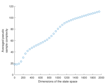
Figure 1: Average pseudo-sample complexity v.s. the state-space dimension.

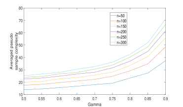
Figure 2: Average pseudo-sample complexity v.s. ‘$\gamma$, for varying state-space dimension

5 Conclusion

We showed existence of invariant ergodic measure for closed-loop switched linear dynamical systems, which are stable in an unbounded subset of the state-space. In addition, we derived non-asymptotic bounds for learning the expected reward from time-averages. With all other parameters fixed, we showed that the sample complexity of learning the expected reward (w.r.t the ergodic invariant measure the closed-loop switched linear dynamical systems mixes to) is linear to the state-space size and inverse quadratic in the approximation error $\epsilon$ (i.e., $\Omega(\frac{n}{\epsilon^{2}})$); hence, extending existing non-asymptotic results to a class of nonlinear dynamical systems. By learning the expected reward instead of a value function parameterized by a discount factor, we provided a non-asymptotic analysis that is valid for applications that require minimizing asymptotic rewards.

6 Acknowledgement

This work is sponsored in part by the AFOSR under award number FA9550-19-1-0169, as well as the NSF CNS-1652544 and CNS-1837499 awards.

Appendix

Claim 1.

For every $(x,y)\in\mathcal{D}$, where $\mathcal{D}:=\{(x,y)\in\mathbb{R}^{n}\times\mathbb{R}^{n}:V(x)+V(y)\leq\hat{r}\}$ and $\hat{r}$ is defined in  (13), it holds that an $\alpha_{(x,y)}:=\int(f_{x}(z)\land g_{y}(z))dz>0$.

Proof.

As discussed in Section  2 ,it suffices to prove that $f_{x}(z)\land g_{y}(z)>0$ a.e. w.r.t Lebesgue measure on $\mathbb{R}^{n}$.

We identify the following three cases and prove the claim for each case.

Case 1. $\|x\|_{2}\leq\varrho$, $\|y\|_{2}>\varrho$ and without loss of generality (w.l.o.g.) assume that $P(x,\cdot)\thicksim\mathcal{N}(\hat{A}_{j}^{\pi}x,{I}_{n})$ and $P(y,\cdot)\thicksim\mathcal{N}(\hat{A}_{k}^{\pi}x,{I}_{n})$ where $\|\hat{A}_{j}^{\pi}\|_{2}^{2}\leq c$ and $\|\hat{A}_{k}^{\pi}\|_{2}^{2}\leq\gamma<1$. Then it holds that

$$f_{x}(z)\land g_{y}(z) =$$

$$=\frac{1}{(2\pi)^{\frac{n}{2}}} \exp(-\frac{\|z\|_{2}^{2}}{2})\Bigg{(}\exp(-\frac{\|\hat{A}_{j}^{\pi}x\|_{2}^{2}}{2})\exp(-z^{T}\hat{A}_{j}^{\pi}x)\land\exp{(-\frac{\|\hat{A}_{k}^{\pi}y\|_{2}^{2}}{2})}\exp(-z^{T}\hat{A}_{k}^{\pi}y)\Bigg{)}$$

$$>\frac{1}{(2\pi)^{\frac{n}{2}}} \exp(-\frac{\|z\|_{2}^{2}}{2})\Bigg{(}\exp(-\frac{\|\hat{A}_{j}^{\pi}x\|_{2}^{2}}{2})\exp(-z^{T}\hat{A}_{j}^{\pi}x)\land\exp(-\frac{\|y\|_{2}^{2}}{2})\exp(-z^{T}\hat{A}_{k}^{\pi}y)\Bigg{)}$$

$$\geq\frac{1}{(2\pi)^{\frac{n}{2}}} \exp(-\frac{\|z\|_{2}^{2}}{2})\Bigg{(}\exp(-\frac{\|\hat{A}_{j}^{\pi}\|_{2}^{2}\|x\|_{2}^{2}}{2})\exp(-z^{T}\hat{A}_{j}^{\pi}x)\land\exp(-\frac{\|y\|_{2}^{2}}{2})\exp(-z^{T}\hat{A}_{k}^{\pi}y)\Bigg{)}$$

$$=\frac{1}{(2\pi)^{\frac{n}{2}}} \exp(-\frac{\|z\|_{2}^{2}}{2})\exp(-\frac{\|\hat{A}_{j}^{\pi}\|_{2}^{2}\|x\|_{2}^{2}}{2})\Bigg{(}\exp(-z^{T}\hat{A}_{j}^{\pi}x)\land$$

$$\exp(\frac{\|\hat{A}_{j}^{\pi}\|_{2}^{2}\|x\|_{2}^{2}}{2})\exp(-\frac{\|y\|_{2}^{2}}{2})\exp(-z^{T}\hat{A}_{k}^{\pi}y)\Bigg{)}$$

$$\geq\frac{1}{(2\pi)^{\frac{n}{2}}} \exp(-\frac{\|z\|_{2}^{2}}{2})\exp(-\frac{\|\hat{A}_{j}^{\pi}\|_{2}^{2}\|x\|_{2}^{2}}{2})\Bigg{(}\exp(-z^{T}\hat{A}_{j}^{\pi}x)\land$$

$$\exp(\frac{\|\hat{A}_{j}^{\pi}\|_{2}^{2}\|x\|_{2}^{2}}{2})\exp(-\frac{(n+c\varrho^{2})}{\gamma(1-\gamma)})\exp(-z^{T}\hat{A}_{k}^{\pi}y)\Bigg{)},$$ (30)

where the last inequality follows from the fact that $\frac{2(n+c\varrho^{2})}{\gamma(1-\gamma)}\geq\|y\|_{2}^{2}>\varrho^{2}$. Since $(1-\gamma)>0$, we get that the right side of (Proof.) is $>0$ a.e w.r.t Lebesgue measure on $\mathbb{R}^{n}$.

Case 2. $\|x\|_{2}>\varrho$, $\|y\|_{2}>\varrho$ and w.l.o.g let us assume that $P(x,\cdot)\thicksim\mathcal{N}(\hat{A}_{l}^{\pi}x,{I})$ and $P(y,\cdot)\thicksim\mathcal{N}(\hat{A}_{m}^{\pi}x,{I})$, where $\|\hat{A}_{l}^{\pi}\|_{2}^{2}\leq\gamma$ and $\|\hat{A}_{m}^{\pi}\|_{2}^{2}\leq\gamma$. Then, the following holds:

$$f_{x}(z)\land g_{y}(z) =$$

$$=\frac{1}{(2\pi)^{\frac{n}{2}}} \exp(-\frac{\|z\|_{2}^{2}}{2})\Bigg{(}\exp(-\frac{\|\hat{A}_{l}^{\pi}x\|_{2}^{2}}{2})\exp(-z^{T}\hat{A}_{l}^{\pi}x)\land\exp(-\frac{\|\hat{A}_{m}^{\pi}y\|_{2}^{2}}{2})\exp(-z^{T}\hat{A}_{m}^{\pi}y)\Bigg{)}$$

$$\geq\frac{1}{(2\pi)^{\frac{n}{2}}} \exp(-\frac{\|z\|_{2}^{2}}{2})\Bigg{(}\exp(-\gamma\frac{\|x\|_{2}^{2}}{2})\exp(-z^{T}\hat{A}_{l}^{\pi}x)\land\exp(-\gamma\frac{\|y\|_{2}^{2}}{2})\exp(-z^{T}\hat{A}_{m}^{\pi}y)\Bigg{)}$$

$$\geq\frac{1}{(2\pi)^{\frac{n}{2}}} \exp(-\frac{\|z\|_{2}^{2}}{2})\exp(-\frac{n+c\varrho^{2}}{(1-\gamma)})\Bigg{(}\exp(-z^{T}\hat{A}_{l}^{\pi}x)\land\exp(-z^{T}\hat{A}_{m}^{\pi}x)\Bigg{)}.$$ (31)

Here, the last inequality follows from the fact that $\frac{2(n+c\varrho^{2})}{\gamma(1-\gamma)}\geq\|y\|_{2}^{2}>\varrho^{2}$ and $\frac{2(n+c\varrho^{2})}{\gamma(1-\gamma)}\geq\|x\|_{2}^{2}>\varrho^{2}$. Since, $(1-\gamma)>0$, it holds that the right side of (Proof.) is $>0$ a.e w.r.t Lebesgue measure on $\mathbb{R}^{n}$.

Case 3. $\|x\|_{2}\leq\varrho$, $\|y\|_{2}\leq\varrho$ and w.l.o.g we assume that $P(x,\cdot)\thicksim\mathcal{N}(\hat{A}_{u}^{\pi}x,{I})$ and $P(y,\cdot)\thicksim\mathcal{N}(\hat{A}_{o}^{\pi}x,{I})$, where $\|\hat{A}_{u}^{\pi}\|_{2}^{2}\leq C$ and $\|\hat{A}_{o}^{\pi}\|_{2}^{2}\leq C$. Then, it holds that

$$f_{x}(z)\land g_{y}(z) =$$

$$=\frac{1}{(2\pi)^{\frac{n}{2}}} \exp(-\frac{\|z\|_{2}^{2}}{2})\Bigg{(}\exp(-\frac{\|\hat{A}_{u}^{\pi}x\|_{2}^{2}}{2})\exp(-z^{T}\hat{A}_{u}^{\pi}x)\land\exp(-\frac{\|\hat{A}_{o}^{\pi}x\|_{2}^{2}}{2})\exp(-z^{T}\hat{A}_{o}^{\pi}x)\Bigg{)}$$

$$\geq\frac{1}{(2\pi)^{\frac{n}{2}}} \exp(-\frac{\|z\|_{2}^{2}}{2})\Bigg{(}\exp(-\frac{C\|x\|_{2}^{2}}{2})\exp(-z^{T}\hat{A}_{u}^{\pi}x)\land\exp(-\frac{C\|y\|_{2}^{2}}{2})\exp(-z^{T}\hat{A}_{o}^{\pi})\Bigg{)}$$

$$\geq\frac{1}{(2\pi)^{\frac{n}{2}}} \exp(-\frac{\|z\|_{2}^{2}}{2})\exp(-\frac{C\varrho^{2}}{2})\Bigg{(}\exp(-z^{T}\hat{A}_{u}^{\pi}x)\land\exp(-z^{T}\hat{A}_{o}^{\pi}y)\Bigg{)}.$$ (32)

Hence, the right side of (32) is $>0$ a.e w.r.t Lebesgue measure on $\mathbb{R}^{n}$, which concludes the proof. ∎

Proof of Theorem 3

Proof.

Using Theorem 3.1 in Łatuszyński u. a. (2013) we get that

$$\mathbb{E}_{x}(\frac{1}{N}\sum_{i=0}^{N-1}(r(x_{i})-\int r(y)\nu_{\pi}(dy)))^{2}$$

$$\leq\frac{\sigma_{as}^{2}(P,r)}{N}(1+\frac{C_{0}^{2}(P)}{N^{2}}+2\frac{C_{0}(P)}{N})+4\frac{C_{1}(P,r)}{N}\frac{\sigma_{as}(P,r)}{\sqrt{N}}(1+\frac{C_{0}(P)}{N})+4\frac{C_{1}^{2}(P,r)}{N^{2}}.$$ (33)

Now, from Theorem 4.2 and Proposition 4.5 in Łatuszyński u. a. (2013), it follows that

$$4\frac{C_{1}(P,r)}{N}\frac{\sigma_{as}(P,r)}{\sqrt{N}}(1+\frac{C_{0}(P)}{N})\leq 4\frac{c_{10as}}{N\sqrt{N}}(2\pi(\hat{V})+\frac{1-\gamma}{2n}\gamma\|x\|_{2}^{2})\frac{2n}{1-\gamma}\leq 4(\frac{c_{10as}}{N})(\frac{6n+2c\varrho^{2}+\gamma\|x\|_{2}^{2}}{1-\gamma}),$$ (34)

$$4\frac{C_{1}^{2}(P,r)}{N^{2}}\leq 4(\frac{c_{1}^{2}}{N^{2}})(\frac{3n+c\varrho^{2}+\gamma(1-\gamma)\|x\|_{2}^{2}}{1-\gamma}),$$ (35)

$$2\sigma_{as}^{2}(P,r)\frac{C_{0}(P)}{N^{2}}\leq c_{2as0}\frac{\frac{18}{4}n+c^{2}\varrho^{4}+3c\varrho^{2}}{N^{2}(1-\gamma)},$$ (36)

$$\frac{\sigma_{as}^{2}(P,r)}{N}\frac{C_{0}^{2}(P)}{N^{2}}\leq c_{2as20}\frac{\frac{27}{4}n+\frac{3c^{2}\varrho^{2}}{4}+\frac{27c\varrho^{2}}{4}+\frac{c^{3}\varrho^{4}}{4}+\frac{3c^{2}\varrho^{4}}{2}}{(1-\gamma)N^{3}},$$ (37)

$$\frac{\sigma_{as}^{2}(P,r)}{N}\leq(\frac{1+\sqrt{\lambda}}{1-\sqrt{\lambda}}+\frac{2(\sqrt{K_{2}}-\sqrt{\lambda}-\beta)}{\beta(1-\sqrt{\lambda})})\frac{2n}{N(1-\gamma)}\pi(\hat{V})\leq\frac{4(1+\sqrt{\gamma}\sqrt{1-\gamma}\sqrt{2+c\varrho^{2}})}{N\beta(1-\gamma)^{2}}(3n+c\varrho^{2})$$ (38)

Therefore, it holds that

$$\mathbb{P}(|\frac{1}{N}\sum_{i=0}^{N-1}r(x_{i})-\int_{\mathbb{R}^{n}}r(y)\nu_{\pi}(dy)|>\epsilon)\leq\delta\implies\mathbb{E}_{x}\frac{(|\frac{1}{N}\sum_{i=0}^{N-1}(r(x_{i})-\nu_{\pi}(r))|^{2})}{\epsilon^{2}}\leq\delta$$

$$\implies\frac{\frac{\sigma_{as}^{2}(P,r)}{N}(1+\frac{C_{0}^{2}(P)}{N^{2}}+2\frac{C_{0}P}{N})+4\frac{C_{1}(P,r)}{N}\frac{\sigma_{as}(P,r)}{\sqrt{N}}(1+\frac{C_{0}(P)}{N})+4\frac{C_{1}^{2}(P,r)}{N^{2}}}{\epsilon^{2}}\leq\delta$$

$$\implies N\geq\frac{o_{1}(o_{2}n+o_{3}+\gamma\|x\|_{2}^{2})}{(1-\gamma)\delta\beta\epsilon^{2}},$$ (39)

where (39) follows from (34)-(38). $c_{10as}$, $c_{1}^{2}$, $c_{2as0}$ and $c_{2as20}$ are constants that contain $\lambda$ factor, but since we left $\lambda$ as any arbitrary value between $(\gamma,1)$, we ignore writing down the tedious exact form the aforementioned constants. However, $o_{1}$, $o_{2}$ and $o_{3}$ are fixed constants independent of $n$, $\gamma$ and $\lambda$. ∎

References

- Abbasi-Yadkori u. a. (2019) \NAT@biblabelnumAbbasi-Yadkori u. a. 2019 Abbasi-Yadkori, Yasin ; Lazic, Nevena ; Szepesvari, Csaba: Model-Free Linear Quadratic Control via Reduction to Expert Prediction. In: The 22nd International Conference on Artificial Intelligence and Statistics, 2019, S. 3108–3117
- Athreya und Lahiri (2006) \NAT@biblabelnumAthreya und Lahiri 2006 Athreya, Krishna B. ; Lahiri, Soumendra N.: Measure theory and probability theory. Springer Science & Business Media, 2006
- Athreya und Roy (2014) \NAT@biblabelnumAthreya und Roy 2014 Athreya, Krishna B. ; Roy, Vivekananda: When is a Markov chain regenerative? In: Statistics & Probability Letters 84 (2014), S. 22–26
- Bertail und Ciołek (2018) \NAT@biblabelnumBertail und Ciołek 2018 Bertail, Patrice ; Ciołek, Gabriela: New Bernstein and Hoeffding type inequalities for regenerative Markov chains. (2018)
- Bertsekas (1995) \NAT@biblabelnumBertsekas 1995 Bertsekas, Dimitri P.: Dynamic programming and optimal control. Athena scientific Belmont, MA, 1995
- Boucheron u. a. (2013) \NAT@biblabelnumBoucheron u. a. 2013 Boucheron, Stéphane ; Lugosi, Gábor ; Massart, Pascal: Concentration inequalities: A nonasymptotic theory of independence. Oxford university press, 2013
- Douc u. a. (2014) \NAT@biblabelnumDouc u. a. 2014 Douc, Randal ; Moulines, Eric ; Olsson, Jimmy u. a.: Long-term stability of sequential Monte Carlo methods under verifiable conditions. In: The Annals of Applied Probability 24 (2014), Nr. 5, S. 1767–1802
- Eberle (2015) \NAT@biblabelnumEberle 2015 Eberle, Andreas: Markov processes. 2015
- Fazel u. a. (2018) \NAT@biblabelnumFazel u. a. 2018 Fazel, Maryam ; Ge, Rong ; Kakade, Sham ; Mesbahi, Mehran: Global Convergence of Policy Gradient Methods for the Linear Quadratic Regulator. In: International Conference on Machine Learning, 2018, S. 1467–1476
- Folland (2013) \NAT@biblabelnumFolland 2013 Folland, Gerald B.: Real analysis: modern techniques and their applications. John Wiley & Sons, 2013
- Hairer (2006) \NAT@biblabelnumHairer 2006 Hairer, Martin: Ergodic properties of Markov processes. In: Lecture notes (2006)
- Hairer (2010) \NAT@biblabelnumHairer 2010 Hairer, Martin: Convergence of Markov processes. In: Lecture notes (2010)
- van Handel (2014) \NAT@biblabelnumvan Handel 2014 Handel, Ramon van: Probability in high dimension / PRINCETON UNIV NJ. 2014. – Forschungsbericht
- Hao u. a. (2020) \NAT@biblabelnumHao u. a. 2020 Hao, Botao ; Lazic, Nevena ; Abbasi-Yadkori, Yasin ; Joulani, Pooria ; Szepesvari, Csaba: Provably Efficient Adaptive Approximate Policy Iteration. In: arXiv preprint arXiv:2002.03069 (2020)
- Kulik (2015) \NAT@biblabelnumKulik 2015 Kulik, Alexei: Introduction to Ergodic rates for Markov chains and processes: with applications to limit theorems. Bd. 2. Universitätsverlag Potsdam, 2015
- Łatuszyński u. a. (2013) \NAT@biblabelnumŁatuszyński u. a. 2013 Łatuszyński, Krzysztof ; Miasojedow, Błażej ; Niemiro, Wojciech u. a.: Nonasymptotic bounds on the estimation error of MCMC algorithms. In: Bernoulli 19 (2013), Nr. 5A, S. 2033–2066
- Lazaric u. a. (2012) \NAT@biblabelnumLazaric u. a. 2012 Lazaric, Alessandro ; Ghavamzadeh, Mohammad ; Munos, Rémi: Finite-sample analysis of least-squares policy iteration. In: Journal of Machine Learning Research 13 (2012), Nr. Oct, S. 3041–3074
- Oymak (2019) \NAT@biblabelnumOymak 2019 Oymak, Samet: Stochastic Gradient Descent Learns State Equations with Nonlinear Activations. In: Conference on Learning Theory, 2019, S. 2551–2579
- Sarkar u. a. (2019) \NAT@biblabelnumSarkar u. a. 2019 Sarkar, Tuhin ; Rakhlin, Alexander ; Dahleh, Munther A.: Finite-time system identification for partially observed lti systems of unknown order. In: arXiv preprint arXiv:1902.01848 (2019)
- Simchowitz u. a. (2018) \NAT@biblabelnumSimchowitz u. a. 2018 Simchowitz, Max ; Mania, Horia ; Tu, Stephen ; Jordan, Michael I. ; Recht, Benjamin: Learning Without Mixing: Towards A Sharp Analysis of Linear System Identification. In: Conference On Learning Theory, 2018, S. 439–473
- Tu und Recht (2018) \NAT@biblabelnumTu und Recht 2018 Tu, Stephen ; Recht, Benjamin: Least-Squares Temporal Difference Learning for the Linear Quadratic Regulator. In: International Conference on Machine Learning, 2018, S. 5005–5014
- Van Handel (2007) \NAT@biblabelnumVan Handel 2007 Van Handel, Ramon: Stochastic calculus, filtering, and stochastic control. In: Course notes., URL http://www. princeton. edu/rvan/acm217/ACM217. pdf 14 (2007)
- Villani (2008) \NAT@biblabelnumVillani 2008 Villani, Cédric: Optimal transport: old and new. Bd. 338. Springer Science & Business Media, 2008
- Zahavy u. a. (2019) \NAT@biblabelnumZahavy u. a. 2019 Zahavy, Tom ; Cohen, Alon ; Kaplan, Haim ; Mansour, Yishay: Average reward reinforcement learning with unknown mixing times. In: arXiv preprint arXiv:1905.09704 (2019)