GP3: A Sampling-based Analysis Framework for Gaussian Processes

Abstract

Although machine learning is increasingly applied in control approaches, only few methods guarantee certifiable safety, which is necessary for real world applications. These approaches typically rely on well-understood learning algorithms, which allow formal theoretical analysis. Gaussian process regression is a prominent example among those methods, which attracts growing attention due to its strong Bayesian foundations. Even though many problems regarding the analysis of Gaussian processes have a similar structure, specific approaches are typically tailored for them individually, without strong focus on computational efficiency. Thereby, the practical applicability and performance of these approaches is limited. In order to overcome this issue, we propose a novel framework called GP3, general purpose computation on graphics processing units for Gaussian processes, which allows to solve many of the existing problems efficiently. By employing interval analysis, local Lipschitz constants are computed in order to extend properties verified on a grid to continuous state spaces. Since the computation is completely parallelizable, the computational benefits of GPU processing are exploited in combination with multi-resolution sampling in order to allow high resolution analysis.

1 Introduction

Machine learning is increasingly applied in control approaches, where first principle models are not available or expensive to obtain due to the complexity of systems. In order to apply learning based control approaches to real world applications, it is crucial to certify their safety using theoretically rigorous methods. Although there exists a wide variety of machine learning methods, this theoretical analysis is often difficult, such that safe control approaches typically rely on a few, well-understood learning methods.

Gaussian process (GP) regression is such a machine learning method which bases on solid Bayesian foundations. Due to its inherent bias-variance trade-off it allows efficient generalization from few training data, which makes it an appealing method both for control practitioners and theoreticians, and has lead to its increasing use in control. For the control theoretic analysis of Gaussian processes, several approaches have been developed. In (Beckers and Hirche, 2016a, b) stochastic stability and equilibria of Gaussian processes with certain covariance kernels are investigated analytically. Employing numerical quadrature, an efficient method to analyze stability of the posterior mean function of a Gaussian process state space model with squared exponential kernel is developed in (Vinogradska et al., 2017). A statistical learning error analysis of learned MPC control laws is proposed in (Hertneck et al., 2018) to ensure closed-loop stability. By extending the Lyapunov stability conditions on a grid to a continuous state space using Lipschitz continuity, the region of attraction of a Gaussian process state space model is learned in (Berkenkamp et al., 2016). A similar approach is employed to determine the region of attraction of a nonlinear system based on the learned infinite horizon cost function in (Lederer and Hirche, 2019). The Lipschitz constants of the posterior mean function used in these approaches are also of interest themselves, e.g., for computing uniform regression error bounds (Lederer et al., 2019) or in batch parallelization of Bayesian optimization in (González et al., 2016).

Despite of the similarity of many of these problems, each one is based on a separate analysis method, which is typically not optimized for computational efficiency. In order to overcome this issue, we propose a novel framework for the analysis of Gaussian process mean functions called GP3: General Purpose computation on Graphics Processing units for Gaussian Processes. By defining a common problem formulation for many problems, we can employ interval analysis to derive local Lipschitz constants on hyperrectangles covering the region of interest. These local Lipschitz constants allow to extend verified properties on a discrete grid to the whole region of interest such that multi-resolution sampling can be used for efficient analysis. As the Lipschitz constants can be computed independently for each hyperrectangle, the method is parallelized using general purpose graphics processing units in order to exploit the full computational power of modern hardware. We demonstrate the flexibility and efficiency of the GP3 framework by applying it to a region of attraction estimation and a Lipschitz constant bounding problem.

The remaining paper is structured as follows. In Section 2 we define the general property analysis problem. The theoretical background on Gaussian process regression and interval analysis is presented in Section 3. The theoretical foundations of the GP3 framework are explained in Section 4, before it is evaluated in simulations in Section 5.

2 Problem Statement

Consider the posterior mean function $\mu:\mathbb{R}^{d}\rightarrow\mathbb{R}$ of a Gaussian process with continuous covariance kernel $k:\mathbb{R}^{d}\times\mathbb{R}^{d}\rightarrow\mathbb{R}$, a continuous function $g:\mathbb{R}^{d}\rightarrow\mathbb{R}$ for comparison and a continuous state transformation $\bm{f}:\mathbb{R}^{d}\rightarrow\mathbb{R}^{d}$. An abstract problem that finds many practical applications is to find bounds $\epsilon_{1},\epsilon_{2}\in\mathbb{R}_{+}$ on the difference

$$-\epsilon_{1}\leq g(\bm{f}(\bm{x}))-\mu(\bm{x})\leq\epsilon_{2}\quad\forall\bm{x}\in\mathbb{X}$$ (1)

on a compact set $\mathbb{X}\!\subset\!\mathbb{R}^{d}$. Various choices for the functions $\bm{f}(\cdot),g(\cdot)$ immediately come to mind: if we choose $g(\cdot)$ as the function generating the training data of the Gaussian process and set $\bm{f}(\bm{x})\!=\!\bm{x}$ we can determine the maximum learning error. Furthermore, $\bm{g}(\cdot)$ can be the Gaussian process mean $\mu(\cdot)$ itself and $\bm{f}(\cdot)$ can be defined such that it returns the closest point in a discrete set. Thereby the variation of the mean function with respect to the discrete set is analyzed. Finally, we can consider $\bm{f}(\cdot)$ as autonomous, discrete-time dynamics and choose $g(\cdot)\!=\!\mu(\cdot)$, such that we can immediately investigate if the mean function $\mu(\cdot)$ satisfies the second condition of Lyapunov’s theorem. Although this problem formulation offers such a high flexibility, it allows a straight forward, uniform treatment through interval analysis, which we exploit in the following sections.

3 Theoretical Background

3.1 Gaussian Process Regression

Gaussian process regression is a supervised machine learning method, which is frequently applied in control and system identification due to its Bayesian foundations. The Gaussian process distribution assigns to any finite subset $\{\bm{x}_{i},\ldots,\bm{x}_{N}\}\subset\mathbb{X}$ from a continuous input domain $\mathbb{X}\subset\mathbb{R}^{d}$ a joint Gaussian distribution (Rasmussen and Williams, 2006). It is completely defined through the mean function $m:\mathbb{R}^{d}\rightarrow\mathbb{R}$ and the covariance function $k:\mathbb{R}^{d}\times\mathbb{R}^{d}\rightarrow\mathbb{R}$. Although prior information like approximate models can be incorporated as mean function $m(\cdot)$ into GP regression, such knowledge is often not available, such that the mean function $m(\cdot)$ is usually set to zero. We also assume this in the following. In contrast, a wide variety of different covariance functions $k(\cdot,\cdot)$ is applied in GP regression to encode prior information such as smoothness, periodicity and stationarity. Frequently used covariance functions are the squared exponential kernel

$$k_{\mathrm{SE}}(r)=\sigma_{f}^{2}\exp\left(-\frac{1}{2}r^{2}\right)$$ (2)

and the Matérn class kernels

$$k_{m+\frac{1}{2}}(r)=\sigma_{f}^{2}p_{m}(r)\exp\left(-\sqrt{(2m+1)}r\right)$$ (3)

with signal variance $\sigma_{f}^{2}\in\mathbb{R}_{+}$, $p_{m}(\cdot)$ a polynomial of order $m\in\mathbb{N}$ and automatic relevance determination distance (Neal, 1996)

$$r=\sqrt{\sum\limits_{i=1}^{d}\frac{(x_{i}-x_{i}^{\prime})^{2}}{l_{i}^{2}}}$$ (4)

with length scales $l_{i}\in\mathbb{R}_{+}$. Matérn class kernels are commonly used with $m=1$ or $m=2$ which results in the polynomials

$$p_{1}(r) =1+\sqrt{3}r$$ (5)

$$p_{2}(r) =\left(1+\sqrt{5}r+\frac{5}{3}r^{2}\right).$$ (6)

A major reason for their popularity is the fact that a GP with either of these covariance functions is a universal approximator (Steinwart, 2001), i.e., any continuous function can be approximated with arbitrary precision.

GP regression is based on the assumption that the training data set $\mathbb{D}=\{(\bm{x}^{(n)},y^{(n)})\}_{n=1}^{N}$ is generated through noisy observations of a function $h:\mathbb{R}^{d}\rightarrow\mathbb{R}$, i.e.,

$$y^{(i)}=h(\bm{x}^{(i)})+\omega^{(i)},$$ (7)

where $\omega^{(i)}\sim\mathcal{N}(0,\sigma_{n}^{2})$ are i.i.d. random variables. By conditioning the prior joint Gaussian distribution of a prediction $h(\bm{x})$ and the training outputs $y^{(i)}$ on the training data $\mathbb{D}$, we obtain the predictive mean

$$\mu(\bm{x})=\mathbb{E}[h(\bm{x})|\mathbb{D},\bm{x}]=\bm{k}^{T}(\bm{x})\bm{\lambda},$$ (8)

where

$$\bm{\lambda}=(\bm{K}+\sigma_{n}^{2}\bm{I}_{N})^{-1}\bm{y}$$ (9)

and the data covariance matrix $\bm{K}\in\mathbb{R}^{N\times N}$ and the covariance vector $\bm{k}(\bm{x})\in\mathbb{R}^{N}$ are defined through $K_{ij}=k(\bm{x}^{(i)},\bm{x}^{(j)})$ and $k_{i}(\bm{x})=k(\bm{x}^{(i)},\bm{x})$. The observation noise variance $\sigma_{n}^{2}$, the signal variance $\sigma_{f}^{2}$ and the length scales $l_{i}$ are considered hyperparameters of the GP regression and can be determined by maximization of the log-likelihood (Rasmussen and Williams, 2006).

3.2 Interval Analysis for Property Analysis

Interval analysis is a method to approach the problem of calculating bounds of functions. Instead of operating on exact values, interval analysis uses real compact intervals $[a]=[\underline{a},\bar{a}]=\{x\in\mathbb{R}|\underline{a}\leq x\leq\bar{a}\}$. Basic mathematical operations for intervals are defined as

$$[a]+[b] =[\underline{a}+\underline{b},\overline{a}+\overline{b}],$$ (10)

$$[a]-[b] =[\underline{a}-\overline{b},\overline{a}-\underline{b}],$$ (11)

$$[a]\cdot[b] =[\mathrm{min}\{\underline{a}\underline{b},\underline{a}\overline{b},\overline{a}\underline{b},\overline{a}\overline{b}\},\mathrm{max}\{\underline{a}\underline{b},\underline{a}\overline{b},\overline{a}\underline{b},\overline{a}\overline{b}\}].$$ (12)

A more thorough introduction into operations on intervals can be found, e.g., in (Alefeld and Mayer, 2000).

Based on this interval arithmetic, it is possible to use intervals as inputs to functions $f:\mathbb{R}\rightarrow\mathbb{R}$ and calculate output intervals $[y]=f([x])$, where $\underline{y}$ serves as a lower bound and $\bar{y}$ as an upper bound of the function values on the input interval. It is straight forward to adapt this approach to higher dimensional functions $f:\mathbb{R}^{d}\rightarrow\mathbb{R}$ by considering so called hyperrectangles instead of intervals. A hyperrectangle is completely defined by its center $\bm{c}$ and length parameter $\bm{b}$, such that it defines the multi-dimensional interval $[\bm{c}-\bm{b},\bm{c}+\bm{b}]$ with edge widths $2\bm{b}$. Using a grid of hyperrectangles, interval analysis allows to efficiently expand the validity of (1) on the hyperrectangle centers to the area covered by the hyperrectangles. Using multi-resolution grids as proposed, e.g., in (Bobiti and Lazar, 2018), this enables efficient determination of valid constants $\epsilon_{1}$ and $\epsilon_{2}$ in (1).

4 Sampling-Based Analysis of Gaussian Processes

Due to the strong nonlinearity of typical Gaussian process mean functions, standard interval operations are not directly applicable to their analysis. Therefore, we develop an efficient multi-resolution sampling algorithm for the analysis of Gaussian processes in Section 4.1. As this algorithm requires upper and lower bounds for the derivative of covariance kernels depending on the training data, we investigate such bounds for squared exponential and Matérn class kernels in Section 4.2.

4.1 Multi-resolution Analysis of Gaussian Processes

Gaussian processes exhibit a strongly nonlinear mean function in general. In order to efficiently analyze their mean functions we develop a multi-resolution sampling algorithm in this section. Exploiting Lipschitz continuity we derive a theorem to calculate the bounds $\epsilon_{1}$ and $\epsilon_{2}$ in (1) inside hyperrectangles. In order to evaluate the bound, we determine a local Lipschitz constant of the GP on a hyperrectangle. Due to the sampling structure, the analysis of hyperrectangles can be efficiently parallelized using GPUs in each grid refinement iteration.

The basis of our approach lies in the independent analysis of the bounds $\epsilon_{1}$ and $\epsilon_{2}$ on hyperrectangles. This analysis is founded on the following theorem, which relies on Lipschitz continuity of all involved functions.

Theorem 1

Consider a function $\bm{f}(\cdot)$ with local Lipschitz constant $L_{f}$ and a posterior mean function $\mu(\cdot)$ of a Gaussian process with local Lipschitz constant $L_{\mu}$ on a hyperrectangle with center $\bm{c}$ and edge widths $2\bm{b}$. Furthermore, assume the function $g(\cdot)$ has a local Lipschitz constant $L_{g}$ on the hyperrectangle with center $\bm{f}(\bm{c})$ and edge widths $2L_{f}\bm{b}$. Then, (1) holds with

$$\epsilon_{1} =g(\bm{f}(\bm{c}))-\mu(\bm{c})-(L_{f}L_{g}+L_{\mu})\|\bm{b}\|$$ (13)

$$\epsilon_{2} =g(\bm{f}(\bm{c}))-\mu(\bm{c})+(L_{f}L_{g}+L_{\mu})\|\bm{b}\|$$ (14)

for all $|\bm{x}-\bm{c}|\leq\bm{b}$, where the absolute values and the comparison are performed element-wise.

Due to Lipschitz continuity of $\bm{f}(\cdot)$ and $g(\cdot)$ it follows that

$$|g(\bm{f}(\bm{x}))-g(\bm{f}(\bm{c}))|\leq L_{f}L_{g}\|\bm{b}\|\quad\forall\bm{x}:\|\bm{x}-\bm{c}\|\leq\|\bm{b}\|.$$

Furthermore, Lipschitz continuity of the GP yields

$$|\mu(\bm{x})-\mu(\bm{c})|\leq L_{\mu}\|\bm{b}\|.$$

Applying the triangle inequality we finally obtain the bounds (13) and (14).

The application of this theorem crucially relies on the Lipschitz constant of the GP mean function. The computation of this Lipschitz constant on a hyperrectangle can be performed independently for each hyperrectangle and depends merely on the parameter vector $\bm{\lambda}$, the kernel function $k(\cdot,\cdot)$ and the data points $\bm{x}^{(i)}$, $i=1,\ldots,N$, as shown in the following theorem.

Theorem 2

Consider the posterior mean function $\mu(\cdot)=\bm{k}^{T}(\cdot)\bm{\lambda}$ of a GP with covariance kernel $k(\cdot,\cdot)$ on a hyperrectangle with center $\bm{x}$ and length $2\bm{b}$. Let $\bm{L}_{k,i}^{\partial j}$ denote a vector of partial derivative bounds of the $i$-th element of $\bm{k}(\cdot)$ with respect to $x_{j}$. Then, a local Lipschitz constant of the mean on the hyperrectangle is given by

$$L_{\mu}(\bm{x},\bm{b})=\sqrt{\sum\limits_{j=1}^{d}\max\left\{\left(\sum\limits_{i=1}^{N}\bm{R}(\lambda_{i})\lambda_{i}\bm{L}_{k,i}^{\partial j}\right)^{2}\right\}},$$ (15)

where

$$\bm{R}(\lambda_{i})=\begin{cases}\bm{I}_{2}&\lambda_{i}>0\\ \begin{bmatrix}0&1\\ 1&0\end{bmatrix}&\lambda_{i}\leq 0.\end{cases}$$ (16)

Due to the scalar product of parameter vector $\bm{\lambda}$ and the kernel vector $\bm{k}(\bm{x})$ in (8), the partial derivatives of the mean function are given by

$$\frac{\partial}{\partial x_{j}}\mu(\bm{x})=\begin{bmatrix}\frac{\partial}{\partial x_{j}}k_{1}(\bm{x})&\ldots&\frac{\partial}{\partial x_{j}}k_{N}(\bm{x})\end{bmatrix}\bm{\lambda}.$$

The vectors $\bm{L}_{k,i}^{\partial j}$ contain upper and lower bound on the partial derivatives $\frac{\partial}{\partial x_{j}}k_{i}(\bm{x})$ in the first and second row, respectively. By multiplying these vectors with the matrix $\bm{R}(\lambda_{i})$, the order of elements is changed if $\lambda_{i}$ is negative, such that upper derivative bounds are multiplied with positive $\lambda_{i}$s and lower bounds with negative ones in the first row of the resulting vector. The multiplication is performed in the inverse combination in the second row. By summing up each row, upper and lower bounds on the partial derivatives are obtained. We take the maximum squared value of these two rows as squared Lipschitz constant in the $j$-th direction and finally, calculate the overall Lipschitz $L_{\mu}(\bm{x},\bm{b})$ constant by taking the square root of the sum of squared Lipschitz constants in all directions.

Theorem 1 and Theorem 2 allow for a straightforward implementation and integration in a multi-resolution, GPU parallelized sampling algorithm, which is depicted in Algorithm 1. Initially, a sampling grid is created by dividing the analyzed region $\mathbb{X}$ into $M$ hyperrectangles in line 2, where the centers $\bm{c}_{i}$ are concatenated in $\bm{C}$ and edge-lengths $\bm{b}_{i}$ are concatenated in $\bm{B}$. Generally, any initial sampled grid is possible for this step, since our approach does not crucially depend on it. The grid is refined in line 6 by using an indication value $s_{i}$, which divides hyperrectangles that must be further refined for $s_{i}=\texttt{false}$ from those that require no further refinement. For the refinement procedure itself, several ways are possible in general. A simple method is to resample the grid with smaller hyperrectangle sizes $\bm{B}$ and skip the calculation where $s_{i}=\texttt{true}$ already. Another example for a refinement method is the $2$-refinement used in (Bobiti and Lazar, 2018), where hyperrectangles with $s_{i}=\texttt{false}$ are divided into $2^{d}$ smaller hyperrectangles with new edge widths $\frac{1}{2}\bm{b}_{i}$.

The computation of the bounds $\epsilon_{1},\epsilon_{2}$ based on Theorems 1 and 2 takes place inside the parallelized For (ParFor) loop of line 7. By shifting the execution to a highly parallel GPU, the computation time of the algorithm can be significantly reduced, which is an important feature of this approach. The termination of the refinement process of the algorithm is ensured by setting $s_{i}\!=\!\texttt{true}$, once the bounds $\epsilon_{1},\epsilon_{2}$ inside the hyperrectangle satisfy predefined desired bounding functions $\bar{\epsilon}_{1}(\bm{c}_{i})$ and $\bar{\epsilon}_{2}(\bm{c}_{i})$ or the size $\|\bm{b}_{i}\|$ of the hyperrectangle falls below a specified minimum size $b_{\mathrm{min}}$.

Algorithm 1 Multi-resolution bound calculation

1:0function Bounds($g(\cdot),\mu(\cdot),\mathbb{X},M,\bar{\epsilon}_{1}(\cdot),\bar{\epsilon}_{2}(\cdot),b_{\mathrm{min}}$)

2:-1 $[\bm{C};\bm{B}]\leftarrow$ SamplingGrid($\mathbb{X},M$)

3:-2 $\bm{\epsilon}_{1},\bm{\epsilon}_{2}\leftarrow\texttt{zeros}[\textsf{len}(\bm{C})]$

4:-3 $\bm{s}\leftarrow\texttt{false}[\textsf{len}(\bm{C})]$

5:-4$\textsf{any}(s_{i})=\texttt{false}$

6:-5 $[\bm{C};\bm{B}]\leftarrow$ RefineGrid($\bm{C};\bm{B};s_{i}$)

7:-6$i=1$ to len$(\bm{C})$

8:-7Calculate $L_{\mu}(\bm{c}_{i},\bm{b}_{i})$ using Theorem 2

9:-8Calculate $\epsilon_{1,i},\epsilon_{2,i}$ based on Theorem 1

10:-9$s_{i}\leftarrow(\epsilon_{1,i}\leq\bar{\epsilon}_{1}(\bm{c}_{i})\land\epsilon_{2,i}\leq\bar{\epsilon}_{2}(\bm{c}_{i}))\lor$

11:-10$s_{i}\leftarrow\$$(\|\bm{b}_{i}\|\leq b_{\mathrm{min}})$

12:-11

13:-12

14:-13return  $\bm{C},\bm{\epsilon}_{1},\bm{\epsilon}_{2}$

15:-14

4.2 Derivative Intervals of Kernels

Typical covariance kernels are highly nonlinear functions themselves, which complicates the interval analysis of their derivatives. However, many kernels exhibit a structure such that derivatives are monotonous on large intervals. We exploit this behavior for deriving upper and lower bounds for squared exponential and Matérn class kernels in the following theorem.

Theorem 3

Consider a multivariate squared exponential or Matérn class kernel $k(\cdot)$ with length scale $\bm{l}$ on a hyperrectangle with center $\bm{x}$ and edge lengths $2\bm{b}$. Then, the derivative bounds for a training point $\bm{x}^{(i)}$ with respect to the $j$-th component is given by

$$\bm{L}_{k,i}^{\partial j}=\bm{T}(x_{j}^{(i)}-x_{j})\bm{\kappa}(\bm{x}^{(i)}-\bm{x})$$ (17)

where

$$\bm{\kappa}(\bm{\Delta})=$$ (18)

$$\begin{cases}\begin{bmatrix}-\frac{\partial}{\partial\Delta_{j}}k\left(\rho_{j}\left(\Delta-\overline{\bm{\tau}},|\Delta_{j}|-b_{j}\right)\right)\\ -\frac{\partial}{\partial\Delta_{j}}k\left(\rho_{j}\left(\Delta-\underline{\bm{\tau}},|\Delta_{j}|+b_{j}\right)\right)\end{bmatrix}&|\Delta_{j}|>b_{j}+\tilde{l}_{j}\\[18.0pt] \begin{bmatrix}-\frac{\partial}{\partial\Delta_{j}}k\left(\rho_{j}\left(\Delta-\overline{\bm{\tau}},|\Delta_{j}|+b_{j}\right)\right)\\ -\frac{\partial}{\partial\Delta_{j}}k\left(\rho_{j}\left(\Delta-\underline{\bm{\tau}},|\Delta_{j}|-b_{j}\right)\right)\end{bmatrix}&|\Delta_{j}|<\tilde{l}_{j}-b_{j}\\[18.0pt] \begin{bmatrix}-\frac{\partial}{\partial\Delta_{j}}k\left(\rho_{j}\left(\Delta-\overline{\bm{\tau}},\tilde{l}_{j}\right)\right)\\ \!\min\left\{\!-\frac{\partial}{\partial\Delta_{j}}k\left(\rho_{j}\left(\Delta\!-\!\underline{\bm{\tau}},|\Delta_{j}|\!\pm\!b_{j}\right)\right)\!\right\}\!\end{bmatrix}\!&\!||\Delta_{j}|\!-\!\tilde{l}_{j}|\leq b_{j}\end{cases}$$ (19)

$$\bm{T}(\Delta_{j})=\begin{cases}\bm{I}_{2}&\Delta_{j}>0\\ \begin{bmatrix}0&-1\\ -1&0\end{bmatrix}&\Delta_{j}\leq 0\end{cases},$$ (20)

with modified weighted distance $\rho_{j}(\bm{\Delta},\tilde{\Delta})$, maximum point $\tilde{l}_{j}$, maximum distance $\overline{\bm{\tau}}$, minimum distance $\underline{\bm{\tau}}$ and index set $\mathbb{I}_{j}$ defined as follows

$$\rho_{j}(\!\bm{\Delta},\tilde{\Delta}\!) =\sqrt{\!\frac{\tilde{\Delta}^{2}}{l_{j}^{2}}\!+\!\sum\limits_{i\in\mathbb{I}_{j}}\!\frac{\Delta_{i}^{2}}{l_{i}^{2}}\!}$$ (21)

$$\tilde{l}_{j} =\begin{cases}l_{j}\!&\!\text{squared exponential kernel}\\ \frac{l_{j}}{\sqrt{3}}\!&\!\text{Mat\'{e}rn kernel with }m=1\\ \frac{5\!+\!\sqrt{5}}{10}l_{j}\!&\!\text{Mat\'{e}rn kernel with }m=2\end{cases}$$ (22)

$$\overline{\bm{\tau}} =\min\left\{\|\bm{b}_{\neq j}\|,\|\bm{x}_{\neq j}^{(i)}\!-\!\bm{x}_{\neq j}\|\right\}\frac{\bm{x}^{(i)}\!-\!\bm{x}}{\|\bm{x}_{\neq j}^{(i)}\!-\!\bm{x}_{\neq j}\|}$$ (23)

$$\underline{\bm{\tau}} =\|\bm{b}_{\neq j}\|\frac{\bm{x}\!-\!\bm{x}^{(i)}}{\|\bm{x}_{\neq j}^{(i)}\!-\!\bm{x}_{\neq j}\|}$$ (24)

$$\mathbb{I}_{j} =\{1,\ldots,j-1,j+1,\ldots,d\}.$$ (25)

We start this proof by first showing that (17) holds for the squared exponential before we highlight the differences in the proof for Matérn kernels. Due to the exponent product rule and the automatic relevance determination (4), the derivative of the multivariate squared exponential kernel can be split into

$$\frac{\partial}{\partial x_{j}}k(\bm{x}^{(i)},\bm{x})=-\frac{\partial}{\partial\Delta_{j}}k\left(\frac{|\Delta_{j}|}{l_{j}}\right)k\left(\sqrt{\sum\limits_{i\in\mathbb{I}_{j}}\frac{\Delta_{j}^{2}}{l_{i}^{2}}}\right),$$

where $\bm{\Delta}=\bm{x}^{(i)}-\bm{x}$. This separation allows to determine interval bounds for both factors independently and combine the maximizers or minimizers, respectively, with the help of $\rho_{j}(\bm{\Delta},\Delta_{j})$ based on (12). Due to odd symmetry of the univariate derivative, it is sufficient to derive only bounds for the positive real line and obtain the interval bounds for the negative real line by multiplication with $\bm{T}(\Delta_{j})$. The kernel derivative is monotonous on the intervals $[0,l_{j}]$ and $[l_{j},\infty]$ with a maximum at $l_{j}$. Therefore, we obtain three intervals with maximizers $\nu$

$$|\Delta_{j}|>b_{j}+l_{j} :\nu=|\Delta_{j}|-b_{j}$$

$$|\Delta_{j}|<l_{j}-b_{j} :\nu=|\Delta_{j}|+b_{j}$$

$$||\Delta_{j}|-l_{j}|\leq b_{j} :\nu=l_{j}$$

which can be analogously obtained for the minimizers. The multivariate kernel is trivially maximized by considering the minimal distance to the training point, which is given by $\bm{\Delta}-\overline{\bm{\tau}}$, while it is minimized by $\bm{\Delta}-\underline{\bm{\tau}}$. Therefore, (17) provides an upper and lower bound for the derivative of the squared exponential kernel on the hyperrectangle and we proceed with Matérn class kernels. Although the derivatives of Matérn class kernels cannot be separated as the squared exponential kernel, they exhibit a similar behavior in that they are monotonous in the non-derived directions $i\neq j$. Therefore, we can choose the same maximizer and minimizer in these directions as for the squared exponential kernel. Furthermore, the derivatives of Matérn class kernels exhibit the same odd symmetry in the derived direction $j$ and have two monotonous intervals on the positive real line with maximum at $\tilde{l}_{j}=l_{j}/\sqrt{3}$ for $m=1$ and $\tilde{l}_{j}=(5+\sqrt{5})l_{j}/10$. Therefore, we can upper and lower bound the derivative for Matérn class kernels on the positive real line using (19), which concludes the proof. Although this theorem might appear rather complicated, it allows a straightforward implementation with few conditional operators, which is beneficial for GPU parallelization (Owens et al., 2008). Therefore, it allows efficient, parallelized analysis of Gaussian process mean functions in combination with Theorems 1 and 2.

5 Numerical Evaluation

5.1 Efficiency of the GP3 Framework

In order to demonstrate the advantages of the GP3 framework over a global Lipschitz constant computation and a CPU parallelized implementation, we compare these approaches on the example proposed in (Lederer et al., 2019). A crucial step therein is the derivation of a Lipschitz constant for a posterior mean representing the function

$$f(\bm{x})=1-\sin(x_{1})+\frac{1}{1+\exp(-x_{2})}.$$ (26)

The Gaussian process is trained with $100$ samples which are uniformly spaced over the analyzed region $\mathbb{X}=[-6,4]\times[-4,4]$. We train three GPs with a squared exponential and Matérn kernels with $m=1$ and $m=2$. The hyperparameters obtained via log-likelihood maximization for each of these GPs are depicted in Table 1.

kernel	$\sigma_{n}^{2}$	$\sigma_{f}^{2}$	$\bm{l}$
squared exponential	$0.1$	$0.956$	$[1.762\ 5.537]^{T}$
Matérn with $m=1$	$0.1$	$1.274$	$[3.755\ 15.052]^{T}$
Matérn with $m=2$	$0.1$	$1.012$	$[2.333\ 8.496]^{T}$

Table 1: Hyperparameters of the different covariance kernels

We compute the Lipschitz constants of the posterior mean functions using the GP3 framework for different numbers of hyperrectangles and the naive, global Lipschitz constant proposed in (Lederer et al., 2019). The Lipschitz constants obtained from the GP3 approach are depicted in Figure 1. Since the naive approach yields Lipschitz constants of $343.62$, $245.66$ and $268.20$ for the squared exponential and Matérn kernel with $m=1$ and $m=2$, respectively, the corresponding constant curves are not displayed in the figure. In contrast, the Lipschitz constants obtained by the GP3 approach can provide Lipschitz constants smaller than $20$ with less than $2000$ hyperrectangles. Furthermore, with approximately $10^{6}$ hyperrectangles the Lipschitz constant has almost converged to a constant value.

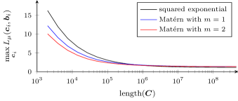
Figure 1: Decrease rate of Lipschitz constants for increasing number of analyzed hyperrectangles

Additionally, we compare the time required to compute the Lipschitz constants on the hyperrectangles with a GPU and CPU parallelization. We compute the Lipschitz constants on a system with a NVIDIA TITAN V GPU, which has $2\!\!:\!\!1$ single to double precision unit ratio, two AMD EPYC $16$-Core CPUs and $1$TB RAM. The speedup of the GPU compared to the CPU parallelization averaged over $10$ runs of both implementations are displayed for the three different covariance kernels in Figure 2. Although we parallelize the Lipschitz constant computation with $64$ threads on the CPU, the GPU parallelization achieves a speedup of at least $30$ for large numbers of hyperrectangles. Merely at low numbers of hyperrectangles the speedup can be in the single digit region due to the computational overhead of GPU computation. Therefore, GP3 allows to exploit the advantages of modern general purpose GPU computing to achieve low computation times, while requiring a reasonable amount of hyperrectangles for convergence of the obtained Lipschitz constant.

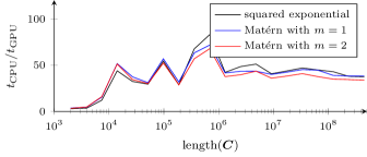
Figure 2: Average speedup of GPU over CPU parallelization over the number of analyzed hyperrectangles

5.2 Region of Attraction for Power Systems

As an example for a problem of the form (1), we analyze the region of attraction of a nonlinear autonomous system. We consider the single machine infinite bus system (Münz and Romeres, 2013)

$$m_{1}\ddot{\phi}_{1}+d_{1}\dot{\phi}_{1}=-a_{12}(\sin(\theta_{1}+\phi_{1})-\sin(\theta_{1})),$$ (27)

which models a synchronous machine with inertia $m_{1}$, damping $d_{1}=20$ and steady state phase $\theta_{1}=\arcsin(0.05)$ as generator bus connected to an infinite bus with $\theta_{2}=\phi_{2}=0$, such that $a_{12}=10$ is the product of the susceptance between both buses and the root mean square voltages $u_{1}$ and $u_{2}$ at bus $1$ and $2$, respectively. For analyzing the regions, where the system is discrete-time stable, we consider the cost of finite time trajectories proposed in (Bobiti and Lazar, 2018) as Lyapunov function, i.e.,

$$V(\bm{x}_{0})=\sum\limits_{k=0}^{K}\bm{x}^{2}(k\Delta t,\bm{x}_{0})$$ (28)

where $\bm{x}(t,\bm{x}_{0})\!=\![\dot{\phi}(t)\ \phi(t)]$ denotes the solution of the differential equation (27) for initial state $\bm{x}_{0}$ and  $\Delta t\!\in\!\mathbb{R}_{+}$ is the sampling time. For determining the states at the sampling times $k\Delta t$, we numerically integrate the system using the Bogacki-Shampine method (Bogacki and Shampine, 1989). In order to avoid the computational complexity of performing this numerical integration for many test points, we compute the value of (28) with $K\!=\!1000$ and $\Delta t\!=\!0.01$ only for $N\!=\!1024$ initial states $\bm{x}_{0}$ uniformly spread over the rectangle $\mathbb{X}\!=\![-5,5]^{2}$ and train a Gaussian process with the data to obtain a learned Lyapunov function $\tilde{V}(\cdot)\!=\!\mu(\cdot)$.

In order to analyze the region of attraction of the system, we follow the approach proposed in (Lederer and Hirche, 2019). First, we determine the regions $\mathbb{W}$ of the state space satisfying the inequality

$$\Delta V(\bm{x}_{0})=\tilde{V}(\bm{x}(\Delta t,\bm{x}_{0}))-\tilde{V}(\bm{x}_{0})\leq 0,$$ (29)

which corresponds to verifying (1) with $\epsilon_{1}=\infty$, $\epsilon_{2}=0$, $g(\cdot)=\mu(\cdot)$ and $\bm{f}(\cdot)=\bm{x}(\Delta t,\cdot)$. Based on the decrease region $\mathbb{W}$, the region of attraction is a level set of the learned Lyapunov given by

$$\mathbb{V}=\{\bm{x}\in\mathbb{X}:\tilde{V}(\bm{x})\leq\min\limits_{\bm{x}\in\mathbb{X}:\Delta\tilde{V}(\bm{x})>0}\tilde{V}(\bm{x})\},$$ (30)

which can also be determined using the GP3 framework. Since the Lipschitz based analysis of our approach does not allow the verification of the decrease condition close to the origin, we assume stability in a ball around $\bm{0}$ with radius $r=0.1$ similarly as in (Lederer and Hirche, 2019).

We apply Alg. 1 with minimal size $b_{\min}=10^{-9}$ of the hyperrectangles and a conservative Lipschitz constant $L_{f}=20$ to both problems. The resulting decrease region $\mathbb{W}$ as well as region of attraction $\mathbb{V}$ of the single machine infinite bus system are illustrated in Fig. 3. Additionally, an estimate of the region of attraction $\mathbb{V}_{\mathrm{num}}$ obtained through examining the convergence of trajectories after $10^{4}$ simulation steps for $4000$ initial states $\bm{x}_{0}$ is depicted. The verified decrease region is different from the approximated true region of attraction $\mathbb{V}_{\mathrm{num}}$ at its boundary. Due to the saw tooth behavior at the boundary of the verified decrease region $\mathbb{W}$, the resulting region of attraction $\mathbb{V}$ is smaller than the numerical approximation $\mathbb{V}_{\mathrm{num}}$. However, this underestimation results mainly from imprecision of the learning, while the GP3 approach allows to analyze the Gaussian process very accurately, since the boundary of $\mathbb{V}$ visually touches the boundary of $\mathbb{W}$ at $\bm{x}=[1.2\ 1.7]^{T}$. Therefore, better estimates of the region of attraction can easily be obtained by training the Gaussian process with more data of the discrete-time Lyapuonv function (28).

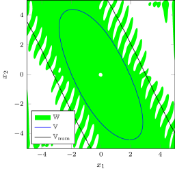
Figure 3: Lyapunov decrease region $\mathbb{W}$ and region of attraction $\mathbb{V}$ obtained with Alg. 1 as well as numerically approximated region of attraction $\mathbb{V}_{\mathrm{num}}$ for the single machine infinite bus system

6 Conclusion

This paper introduces a novel framework for the analysis of Gaussian process mean functions called GP3: general purpose computation on graphics processing units for Gaussian processes. Based on interval analysis to compute local Lipschitz constants, the posterior mean function is analyzed using multi-resolution sampling. Due independence of the computations for each sample, the method can be parallelized on a GPU for computational efficiency. In order to demonstrate the computational benefits of the GP3 framework, it is applied to a Lipschitz constant bounding and a region of attraction estimation problem.

References

- Alefeld and Mayer (2000) Alefeld, G. and Mayer, G. (2000). Interval analysis: theory and applications. Journal of Computational and Applied Mathematics, 121, 421–464.
- Beckers and Hirche (2016a) Beckers, T. and Hirche, S. (2016a). Equilibrium distributions and stability analysis of Gaussian Process State Space Models. In Proceedings of the IEEE Conference on Decision and Control, 6355–6361.
- Beckers and Hirche (2016b) Beckers, T. and Hirche, S. (2016b). Stability of Gaussian Process State Space Models. In Proceedings of the European Control Conference, 2275–2281.
- Berkenkamp et al. (2016) Berkenkamp, F., Moriconi, R., Schoellig, A.P., and Krause, A. (2016). Safe Learning of Regions of Attraction for Uncertain, Nonlinear Systems with Gaussian Processes. In Proceedings of the IEEE Conference on Decision and Control, 4661–4666.
- Bobiti and Lazar (2018) Bobiti, R. and Lazar, M. (2018). Automated-Sampling-Based Stability Verification and DOA Estimation for Nonlinear Systems. IEEE Transactions on Automatic Control, 63(11), 3659–3674.
- Bogacki and Shampine (1989) Bogacki, P. and Shampine, L.F. (1989). A 3(2) pair of Runge - Kutta formulas. Applied Mathematics Letters, 2(4), 321–325.
- González et al. (2016) González, J., Dai, Z., Hennig, P., and Lawrence, N.D. (2016). Batch Bayesian Optimization via Local Penalization. In Proceedings of the International Conference on Artificial Intelligence and Statistics, 648–657.
- Hertneck et al. (2018) Hertneck, M., Köhler, J., Trimpe, S., and Allgöwer, F. (2018). Learning an Approximate Model Predictive Controller with Guarantees. IEEE Control Systems Letters, 2(3), 543–548.
- Lederer and Hirche (2019) Lederer, A. and Hirche, S. (2019). Local Asymptotic Stability Analysis and Region of Attraction Estimation with Gaussian Processes. In Proceedings of the IEEE Conference on Decision and Control.
- Lederer et al. (2019) Lederer, A., Umlauft, J., and Hirche, S. (2019). Uniform Error Bounds for Gaussian Process Regression with Application to Safe Control. In Advances in Neural Information Processing Systems.
- Münz and Romeres (2013) Münz, U. and Romeres, D. (2013). Region of attraction of power systems. IFAC Proceedings Volumes, 46(27), 49–54.
- Neal (1996) Neal, R.M. (1996). Lecture Notes in Statistics: Bayesian Learning for Neural Networks.
- Owens et al. (2008) Owens, J.D., Houston, M., Luebke, D., Green, S., Stone, J.E., and Phillips, J.C. (2008). GPU Computing. Proceedings of the IEEE, 96(5), 879–899.
- Rasmussen and Williams (2006) Rasmussen, C.E. and Williams, C.K.I. (2006). Gaussian Processes for Machine Learning. The MIT Press, Cambridge, MA.
- Steinwart (2001) Steinwart, I. (2001). On the Influence of the Kernel on the Consistency of Support Vector Machines. Journal of Machine Learning Research, 2, 67–93.
- Vinogradska et al. (2017) Vinogradska, J., Bischoff, B., Nguyen-Tuong, D., and Peters, J. (2017). Stability of Controllers for Gaussian Process Dynamics. Journal of Machine Learning Research, 18, 1–37.