Learning Stable Nonparametric Dynamical Systems with Gaussian Process Regression

Abstract

Modelling real world systems involving humans such as biological processes for disease treatment or human behavior for robotic rehabilitation is a challenging problem because labeled training data is sparse and expensive, while high prediction accuracy is required from models of these dynamical systems. Due to the high nonlinearity of problems in this area, data-driven approaches gain increasing attention for identifying nonparametric models. In order to increase the prediction performance of these models, abstract prior knowledge such as stability should be included in the learning approach. One of the key challenges is to ensure sufficient flexibility of the models, which is typically limited by the usage of parametric Lyapunov functions to guarantee stability. Therefore, we derive an approach to learn a nonparametric Lyapunov function based on Gaussian process regression from data. Furthermore, we learn a nonparametric Gaussian process state space model from the data and show that it is capable of reproducing observed data exactly. We prove that stabilization of the nominal model based on the nonparametric control Lyapunov function does not modify the behavior of the nominal model at training samples. The flexibility and efficiency of our approach is demonstrated on the benchmark problem of learning handwriting motions from a real world dataset, where our approach achieves almost exact reproduction of the training data.

1 Introduction

Identification of models for systems involving humans is a highly relevant problem in many fields such as medicine, where dynamical systems can be used to model the progression of a disease, and robotic rehabilitation, where models of the human behavior can be used to maximize the training efficiency. Major difficulties in these modelling problems typically are a high nonlinearity of real world systems, the absence of first principle models and sparsity of the expensive data (Pentland and Liu, 1999). Therefore, parametric models are generally not capable of representing these complex system appropriately.

As a more flexible solution, data-driven approaches, which can extract necessary information automatically from training data, have gained increasing attention for modeling nonlinear systems, since they exhibit sufficient flexibility to adapt their complexity to the observed data and only require marginal prior knowledge. Although classical system identification literature has considered the problem of determining stable models, see, e.g, (Lacy and Bernstein, 2003), the combination of machine learning techniques and control theory has led to a variety of new approaches recently. A common method is to adapt standard machine learning approaches using Lyapunov stability constraints during model parameter optimization. Using a quadratic Lyapuonv function, this method has been applied to Gaussian mixture models in the stable estimator of dynamical systems approach proposed by Khansari-Zadeh and Billard (2011), and is further improved in (Figueroa and Billard, 2018) by employing additional prior distributions, which ensure physical consistency. The constrained optimization method has also been used in combination with neural networks (Neumann et al., 2013), where the flexibility of the model can be improved by learning the Lyapunov function with a separate neural network (Lemme et al., 2014). Since this constrained training approach can have negative effects on the learning performance, it has been proposed to learn a possibly unstable nominal model and a control Lyapunov function (CLF) separately, such that a virtual control can be determined based on the CLF to stabilize the nominal model (Mohammad Khansari-Zadeh and Billard, 2014). This approach has been pursued with different Lyapunov functions, such as the weighted sum of asymmetric quadratic functions (Mohammad Khansari-Zadeh and Billard, 2014) and sums of squares (Umlauft et al., 2017). Furthermore it has been extended to achieve risk-sensitive behavior by considering the model uncertainty due to sparsity of data (Pöhler et al., 2019).

Although the existing methods ensure stable trajectories and achieve low reproduction errors on many practical examples, there are no guarantees on the achievable expressiveness using a certain model. As this issue arises mainly due to the use of parametric Lyapunov functions, we develop a novel, nonparametric Lyapunov function which can be learned from data using Gaussian process regression. We employ a Gaussian process state space model (GP-SSM) as nominal model, and show that it can learn dynamical systems accurately on training data. By stabilizing the GP-SSM based on the nonparametric control Lyapunov function, we prove that the resulting model is capable of reproducing observed data exactly, while being globally asymptotically stable. The flexibility of the approach is demonstrated in learning dynamical systems from a real world dataset, and compared to existing methods.

The remainder of this paper is organized as follows. In Section 2, we describe the considered problem. Section 3 explains our approach to learn a stable dynamical system which reproduces observed data. The method is compared to existing approaches on real world data in Section 4.

2 Problem Statement

Consider a nonlinear, discrete-time dynamical system

$$\bm{x}_{k+1}=\bm{f}(\bm{x}_{k})$$ (1)

which is asymptotically stable on the continuous valued state space $\mathbb{X}\subset\mathbb{R}^{d}$. Furthermore, assume that the function $\bm{f}(\cdot)$ is unknown and that consecutive measurements of the states are taken such that we obtain a training data set $\mathbb{D}=\{(\bm{x}_{k}^{(m)},\bm{x}_{k+1}^{(m)})\}_{m=1}^{M}$ with $M\in\mathbb{N}$ data pairs. We will make use of the following assumption.

Assumption 1

The function $\bm{f}(\cdot)$ defines an asymptotically stable system (1) on the compact set $\mathbb{X}\subset\mathbb{R}^{d}$.

We want to estimate a model based on the observed data, which exhibits the posed assumptions on stability. Therefore, the goal is to derive a stable model of the unknown dynamical system, which maximizes the accuracy of the reproduced training trajectories by reproducing the observed data $(\bm{x}_{k}^{(m)},\bm{x}_{k+1}^{(m)})$ exactly.

3 Stabilization of Gaussian Process State Space Models

For learning stable dynamical systems capable of reproducing observations, we follow the control Lyapunov function approach proposed in (Umlauft et al., 2017). For this virtual stabilization method, we separately learn a nominal system model $\bm{\mu}:\mathbb{X}\rightarrow\mathbb{R}^{d}$ and a control Lyapunov function $V:\mathbb{X}\rightarrow\mathbb{R}_{+}$ from the training data. For a prediction, we determine the optimal, stabilizing virtual control $\bm{u}^{*}(\bm{x})$ for the nominal model $\bm{\mu}(\cdot)$ based on the control Lyapunov function $V(\cdot)$, which minimally modifies the nominal model, and define the stable model as

$$\hat{\bm{f}}(\bm{x})=\bm{\mu}(\bm{x})+\bm{u}^{*}(\bm{x}).$$ (2)

Since we consider scenarios with sparse data, we employ Gaussian process (GP) regression, whose implicit bias-variance trade-off avoids overfitting and hence, provides high prediction accuracy with few training samples. We consider deterministic systems and therefore, we use noise-free Gaussian process state space models as nominal model in contrast to the approach proposed in (Umlauft et al., 2017). We show that the noise-free GP-SSMs are capable of reproducing the training data exactly under weak assumptions in Section 3.1. In Section 3.2 we propose a novel method to learn a nonparametric control Lyapunov function from training data based on Gaussian process regression, which is guaranteed to converge along the training data. Finally, we show that a stabilizing control can be obtained via a constrained optimization and equals zero for all training data in Section 3.3. Therefore, we obtain an asymptotically stable model (2), which is capable of reproducing observed data exactly.

3.1 Gaussian Process State Space Models

Gaussian processes are a powerful machine learning tool for approximating nonlinear functions (Rasmussen and Williams, 2006). A GP is a stochastic process on the continuous input domain $\mathbb{X}$ such that each finite subset $\{\bm{x}_{1},\ldots,\bm{x}_{N}\}\subset\mathbb{X}$ is assigned a joint Gaussian distribution. This view is equal to a consideration as distribution over functions, which is typically expressed through

$$f(\bm{x})\sim\mathcal{GP}(m(\bm{x}),k(\bm{x},\bm{x}^{\prime}))$$ (3)

with prior mean and covariance function

$$m(\bm{x}) =E[f(\bm{x})]$$ (4)

$$k(\bm{x},\bm{x}^{\prime}) =E[(f(\bm{x})-m(\bm{x}))(f(\bm{x}^{\prime})-m(\bm{x}^{\prime}))].$$ (5)

A GP is completely specified by its mean function $m(\cdot)$ and covariance kernel $k(\cdot,\cdot)$. The mean function allows to include prior knowledge in the form of approximate or parametric models. While such models exist for some applications, we do not assume their availability in the following and set the prior mean function to $m(\bm{x})=0$ without loss of generality. The covariance kernel $k(\cdot,\cdot)$ is used to encode more abstract prior knowledge such as information about the smoothness of the regressed function and determines which functions can be approximated properly with a Gaussian process. Probably the most commonly used kernel is the squared exponential (SE) kernel with automatic relevance determination

$$k(\bm{x},\bm{x^{\prime}})=\sigma_{f}^{2}\mathrm{exp}\bigg{(}-\frac{1}{2}\sum\limits_{i=1}^{d}\bigg{(}\frac{x_{i}-x^{\prime}_{i}}{l_{i}}\bigg{)}^{2}\bigg{)},$$ (6)

where $\sigma_{f}^{2}\in\mathbb{R}_{+}$ is the signal variance and $l_{i}\in\mathbb{R}_{+},\forall i=1,\ldots,d$ are the length-scale parameters. These variables are concatenated in a hyperparameter vector $\bm{\psi}=[l_{1}\ldots l_{d}\ \sigma_{f}]^{T}$. The squared exponential kernel is a universal kernel in the sense of (Steinwart, 2001) which means that it allows to approximate continuous functions arbitrarily well. Therefore, Gaussian process regression with this kernel is capable of learning many typical dynamics.

We employ $d$ independent GPs to model a dynamical system with $d$-dimensional state space, such that the $i$-th component is denoted by

$$f_{i}(\bm{x})\sim\mathcal{GP}(0,k_{i}(\bm{x,x}^{\prime})).$$ (7)

Predictions with this model can be calculated by conditioning the prior GPs (7) on the given training set $\mathbb{D}=\{\bm{x}_{k}^{(n)},\bm{x}_{k+1}^{(n)}\}_{i=1}^{N}$. The conditional expectation $\mu(\cdot)$ can be calculated analytically using linear algebra. For this reason, we define target vectors

$$\bm{y}_{i}=[x_{k+1,i}^{(1)}\ \ldots\ x_{k+1,i}^{(N)}].$$ (8)

Then, the predictive mean is given by

$$\mu_{i}(\bm{x})=\bm{k}_{i}(\bm{x})\bm{K}_{i}^{-1}\bm{y}_{i}$$ (9)

with $K_{i,n,m}=k_{i}(\bm{x}_{k}^{(n)},\bm{x}_{k}^{(m)})$ and $k_{i,n}=k_{i}(\bm{x},\bm{x}_{k}^{(n)})$.

Remark 1

The matrix inverse in (9) theoretically always exists for the squared exponential kernel if there is no repeated entry in the input data, i.e., $\bm{x}_{k}^{(n)}\!\neq\!\bm{x}_{k}^{(m)}$, $\forall n\!\neq\!m$, due to the fact that this kernel is universal (Steinwart, 2001). However, a small regularizer, typically called observation noise variance $\sigma_{\mathrm{on}}^{2}$, can be added on the diagonals of $\bm{K}_{i}$ in order to avoid numerically ill-conditioned inversions. This regularizer has typically a small effect on the prediction since the resulting mean squared prediction error is smaller than the noise variance (Rasmussen and Williams, 2006).

The hyperparameters $\bm{\psi}_{i}$ of the Gaussian processes $f_{i}(\cdot)$ can be obtained by independently maximizing the log-likelihood

$$\log p(\bm{y}_{i}|\bm{X}_{i})\!=\! -\!\frac{1}{2}\bm{y}_{i}^{T}\!\bm{K}_{i}^{-\!1}\!\bm{y}_{i}\!-\!\frac{1}{2}\!\log\det(\!\bm{K}_{i}\!)\!-\!\frac{N}{2}\!\log 2\pi\!,\!$$ (10)

where $\bm{X}=[\bm{x}_{k}^{(1)}\ \ldots\ \bm{x}_{k}^{(N)}]$ denotes the input training data matrix. This optimization problem is typically solved using gradient based approaches (Rasmussen and Williams, 2006), even though it is generally non-convex.

We use the posterior mean function $\bm{\mu}(\cdot)$ defined through (9) to define a nominal dynamical model

$$\bm{x}_{k+1}=\bm{\mu}(\bm{x}_{k})$$ (11)

which is generally not asymptotically stable. However, training samples are reproduced exactly such that we obtain the following result.

Lemma 1

Consider a training data set $\mathbb{D}\!=\!\{\!(\!\bm{x}_{k}^{(m)}\!\!\!,\bm{x}_{k+1}^{(m)}\!)\!\}_{m\!=\!1}^{M}$ generated by an unknown dynamical system (1), which has a stable equilibrium at the origin. Furthermore, assume that the training data set is augmented by adding the pair $(\bm{0},\bm{0})$. Then, a Gaussian process state space model trained with this training data set reproduces the training data exactly and has an equilibrium at the origin.

Performing the prediction for all training inputs $\bm{x}_{k}^{(m)}$ jointly yields

$$\mu_{i}(\bm{X}_{k})=\bm{K}_{i}\bm{K}_{i}^{-1}\bm{y}_{i}=\bm{y}_{i},$$

where $\mu_{i}(\bm{X}_{k})=[\mu_{i}(\bm{x}_{k}^{(1)})\ \ldots\ \mu_{i}(\bm{x}_{k}^{(M)})\ \mu_{i}(\bm{0})]$ and the inverse is well defined due to the fact that we consider a deterministic function $\bm{f}(\cdot)$ such that $\bm{x}_{k+1}^{(m)}\neq\bm{x}_{k+1}^{(m^{\prime})}$, $\forall m\neq m^{\prime}$. Furthermore, we have the identity

$$[\bm{y}_{1}\ \ldots\ \bm{y}_{d}]^{T}=[\bm{x}_{k+1}^{(1)}\ \ldots\ \bm{x}_{k+1}^{(M)}\ \bm{0}]$$

due to the definition of the data set $\mathbb{D}$. Therefore, the training data is reproduced exactly by the nominal system (11). Finally, the equilibrium at the origin follows from the additional training pair $(\bm{0},\bm{0})$ due to (Umlauft et al., 2018). The exact reproduction of data regardless of their complexity is a major advantage of the nonparametric GP modeling approach. However, this reproduction is only possible, if the training data can be considered noise-free, which is exploited in the proof as the property $\bm{x}_{k+1}^{(m)}\!\neq\!\bm{x}_{k+1}^{(m^{\prime})}$. In applications with few training data such as medical applications or human-robot interaction, this condition is typically satisfied due to the sparsity of the data. Therefore, it is not a severe restriction.

Remark 3.1

Since we only focus on deterministic systems in our approach, the variance of the next state $\bm{x}_{k+1}$ is not of primary interest in this paper. However, it could be used to determine regions of the state space $\mathbb{X}$, which require more training data in order to provide a good model of the dynamical system.

3.2 Learning Nonparametric Control Lyapunov Functions

Although exact reproduction of the data is possible using GP-SSMs, this does not imply that the stabilized system (2) also exhibits superior reproduction performance. This is due to the fact that an insufficiently flexible parameterization of the control Lyapunov function $V(\cdot)$ might not allow the decrease of $V(\cdot)$ along all training samples. However, the required flexibility is difficult to determine a priori with parametric functions such as sums of squares or weighted sum of asymmetric quadratic functions (Umlauft et al., 2017). Therefore, we propose to learn a control Lyapunov function from data based on Gaussian process regression to exploit the flexibility of a fully nonparametric approach. Since we do not have any target values for the supervised learning, we cannot directly apply the GP regression approach. Therefore, we approximate the infinite horizon cost $\tilde{V}_{\infty}(\bm{x})=\sum_{k=1}^{\infty}l(\bm{f}^{k}(\bm{x}))$, where $\bm{f}^{k}(\cdot)$ denotes the $k$-times application of the dynamics $\bm{f}(\cdot)$ and $l:\mathbb{R}^{d}\rightarrow\mathbb{R}_{+}$ is a chosen stage cost, by transforming the Bellman equation at training points into a regression problem as proposed in (Lederer and Hirche, 2019). This is formalized in the following lemma.

Lemma 2

Consider the approximate infinite horizon cost

$$V_{\infty}(\bm{x})=\bm{\lambda}^{T}(\bm{k}(\bm{X}_{k},\bm{x})-\bm{k}(\bm{X}_{k+1},\bm{x})),$$ (12)

with positive definite stage cost $l:\mathbb{R}^{d}\rightarrow\mathbb{R}_{+}$, training points $\bm{X}_{k}=[\bm{x}_{k}^{(1)}\ \ldots\ \bm{x}_{k}^{(M)}]$, $\bm{X}_{k+1}=[\bm{x}_{k+1}^{(1)}\ \ldots\ \bm{x}_{k+1}^{(M)}]$ and

$$\bm{k}(\bm{X},\bm{x}) =\left[k(\bm{x}^{(1)},\bm{x})\ \ldots\ k(\bm{x}^{(M)},\bm{x})\right]^{T}$$ (13)

$$\bm{\lambda} =\bm{\kappa}^{-1}[l(\bm{x}_{k+1}^{(1)})\ \ldots\ l(\bm{x}_{k+1}^{(M)})]^{T},$$ (14)

where the elements of the invertible matrix $\bm{\kappa}\in\mathbb{R}^{M\times M}$ are defined using the squared exponential kernel $k(\cdot,\cdot)$ as

$$\kappa_{mn} =k\left(\bm{x}_{k}^{(m)},\bm{x}_{k}^{(n)}\right)-k\left(\bm{x}_{k+1}^{(m)},\bm{x}_{k}^{(n)}\right)$$

$$-k\left(\bm{x}_{k}^{(m)},\bm{x}_{k+1}^{(n)}\right)+k\left(\bm{x}_{k+1}^{(m)},\bm{x}_{k+1}^{(n)}\right).$$ (15)

Then, the control Lyapunov function

$$V(\bm{x})=l(\bm{x})+\max\{0,V_{\infty}(\bm{x})+V_{\infty}(\bm{0})\}$$ (16)

is positive definite and decreasing along the training data, i.e., $V(\bm{x}_{k}^{(m)})\!\geq\!V(\bm{x}_{k+1}^{(m)})$, $\forall m\!=\!1,\ldots,M$.

Since $l(\cdot)$ is a positive definite function, $V(\cdot)$ is positive due to its definition (16). Hence, it remains to show the decrease along the training data. For this reason, we first consider the exact infinite horizon cost function $\tilde{V}_{\infty}(\cdot)$, which satisfies the Bellman equation

$$\tilde{V}_{\infty}(\bm{x})-\tilde{V}_{\infty}(\bm{f}(\bm{x}))=l(\bm{f}(\bm{x})).$$

Due to (Lederer and Hirche, 2019), a function satisfying this equation on a finite set of pairs $(\bm{x},\bm{f}(\bm{x}))$ can be obtained through noiseless GP regression with the kernel

$$\tilde{k}(\bm{x},\bm{x}^{\prime})\!=\!k(\bm{x},\!\bm{x}^{\prime})\!-\!k(\!\bm{f}(\bm{x}),\!\bm{x}^{\prime})\!-\!k(\bm{x},\!\bm{f}(\bm{x}^{\prime})\!)\!+\!k(\!\bm{f}(\bm{x}),\!\bm{f}(\bm{x}^{\prime})\!)$$

and output training data $\bm{y}\!=\![l(\bm{x}_{k+1}^{(1)})\ \ldots\ l(\bm{x}_{k+1}^{(M)})]^{T}\!$, where invertibility of the matrix $\bm{\kappa}$ defined through (15) is guaranteed due to the usage of the universal squared exponential kernel. This follows directly from a representation of $\tilde{V}_{\infty}(\cdot)$ in the feature space associated with the kernel $k(\cdot,\cdot)$ and the linearity of this representation. Substituting the obtained regression result into the original feature space representation of $\tilde{V}_{\infty}(\cdot)$ directly yields (12). Since the approximate infinite horizon cost (12) is guaranteed to satisfy the Bellman equation on the training pairs, the approximated cost $l(\bm{x})+V_{\infty}(\bm{x})$ is decreasing along the training data. Since this property is shift invariant, i.e., adding a constant to (12) does not change the decrease along training data, (12) is not guaranteed to be positive for all $\bm{x}\neq\bm{0}$. Therefore, we enforce $V(\bm{0})=0$ by adding the value of (12) evaluated at the origin and exclude obvious regression errors by setting negative values of the shifted approximate infinite horizon $V_{\infty}(\bm{x})+V_{\infty}(\bm{0})$ to $0$. Since regression errors do not occur on the training samples, the decrease along training data is guaranteed for (16) and the theorem is proven.

The hyperparameters of the control Lyapunov function $V(\cdot)$ can be obtained via the standard approach of maximizing the log-likelihood (10). However, if we assume a parameterized stage cost $l_{\theta}(\cdot)$, we can optimize jointly with respect to hyperparameters $\bm{\psi}$ and cost parameters $\bm{\theta}$

$$\min\limits_{\bm{\psi},\bm{\theta}}\log p(\bm{l}_{\theta}(\bm{X}_{k+1})|\bm{X}_{k+1},\bm{X}_{k}),$$ (17)

where the log-likelihood is given by

$$\log p(\bm{l}_{\theta}(\bm{X}_{k+1})|\bm{X}_{k+1},\bm{X}_{k})=$$

$$-\!\frac{1}{2}\bm{l}_{\theta}^{T}(\bm{X}_{k+1})\bm{\kappa}^{-1}\bm{l}_{\theta}(\bm{X}_{k+1})\!-\!\frac{1}{2}\log(|\bm{\kappa}|)\!-\!\frac{N}{2}\log(2\pi)$$ (18)

with the abbreviation $\bm{l}_{\theta}(\bm{X}_{k+1})=\big{[}l_{\theta}(\bm{x}_{k+1}^{(1)})\ \ldots\ l_{\theta}(\bm{x}_{k+1}^{(M)})\big{]}$. This approach exhibits the advantage that the highly local approximate infinite horizon cost $V_{\infty}(\cdot)$, which is typically nonzero only in the proximity of training data, and the global parametric stage cost $l(\cdot)$ are jointly adapted to the data.

Remark 3.2

While we assume GPs with squared exponential kernels in this article, all theoretical results are directly applicable to arbitrary universal kernels (Steinwart, 2001).

Remark 3.3

Although the Lyapunov function $V(\cdot)$ depends on the hyperparameters $\bm{\psi}$ and the stage cost parameters $\bm{\theta}$, the fundamental properties such as the decreasing value along the training data are not influenced by them. Therefore, the Lyapunov function $V(\cdot)$ is considered nonparametric. However, the behavior away from the training data crucially depends on the hyperparameters such that the hyperparameter optimization (18) is an important step in obtaining suitable hyperparameters.

3.3 Reproductivity Preserving Stabilization

We pursue the optimization based approach proposed in (Umlauft et al., 2017) to virtually stabilize the nominal system (11) with minimal modification. Within this approach we obtain the stabilizing control $\bm{u}(\bm{x})$ through

$$\bm{u}^{*}(\bm{x})=\arg\mathop{\min}_{\bm{u}}\frac{1}{2}\bm{u}^{T}\bm{u},$$ (19a)

subject to:

$$\begin{split}V(\bm{\mu}(\bm{x})+\bm{u})<V(\bm{x})\qquad&\forall\bm{x}\neq\bm{0}\\ V(\bm{\mu}(\bm{x})+\bm{u})=V(\bm{x})\qquad&\forall\bm{x}=\bm{0},\end{split}$$ (19b)

where $V(\cdot)$ is the nonparametric Lyapunov function (16). Although these non-convex constraints generally prevent guarantees for the global optimality of solutions, this is not a problem since local minima can trivially be obtained by setting $\bm{u}^{*}(\bm{x})=-\bm{\mu}(\bm{x})$. Therefore, asymptotic stability is not affected by the non-convexity of the optimization problem which is exploited in the following theorem.

Theorem 3

The model (2) with nominal model defined through (9) and stabilizing control obtained in (19) based on the nonparametric control Lyapunov function (16) with radially unbounded stage cost $l(\cdot)$ is globally asymptotically stable and reproduces training data exactly, i.e., $\hat{\bm{f}}(\bm{x}_{k}^{(m)})=\bm{x}_{k+1}^{(m)}$, for all $m=0,\ldots,M$.

The function $V(\cdot)$ is positive definite and radially unbounded since the stage cost $l(\cdot)$ also satisfies these conditions. The optimization problem is always feasible since $\bm{u}^{*}(\bm{x})=-\bm{\mu}(\bm{x})$ is a trivial solution and $\|\bm{u}\|^{*}$ is bounded since each mean function of the Gaussian process state space model is bounded, i.e.,

$$|\mu_{i}(\bm{x})|\leq\sigma_{f}^{2}\sqrt{N}||\bm{K_{i}}^{-1}\bm{y}_{i}||\quad\forall i=1,\ldots,d,$$

with $\bm{y}_{i}$ from (8). Because the training set is fixed and generated by a deterministic function $\bm{f}(\cdot)$ the norm of $\bm{K}_{i}^{-1}\bm{y}_{i}$ is a finite constant. Hence, $V(\cdot)$ is a Lyapunov function and the system (2) is globally asymptotically stable. Finally, reproduction of observed training data follows from the fact that $V(\cdot)$ is decreasing along training data as shown in Lemma 2 and the exact reproduction of training data with the nominal model (11) as proven in Lemma 1. Although we use the trivially feasible control $\bm{u}^{*}(\bm{x})=-\bm{\mu}(\bm{x})$ to prove asymptotic stability, it might not lead to good local optima as starting point of numerical optimization. Therefore, we propose to choose as initial point for the numerical optimization the closest training point in the training data set (including the origin) which satisfies the stability conditions. This approach results in weak convergence to the training data as local optima in the proximity of data are more likely to be found.

Remark 3.4

If the stability conditions are already satified by the uncontrolled GP-SSM, the optimal control $\bm{u}^{*}$ is $\bm{0}$. Therefore, there is no need to solve the optimization (19) numerically and computation time can be reduced by directly using the nominal model (11).

4 Experimental Evaluation

In order to demonstrate the flexibility of the proposed nonparametric (NP) Lyapunov function, we compare its performance to the weighted sum of asymmetric quadratic functions (WSAQF) $V_{\rm{WSAQF}}$ (Mohammad Khansari-Zadeh and Billard, 2014) and the sum of squares (SOS) Lyapunov function (Umlauft et al., 2017). We evaluate the performance in learning the motions of the LASA handwriting dataset because it is a well-established benchmark for stable nonlinear dynamical systems, which fosters comparability of the methods. The setting of our simulations is described in Section 4.1, while the results are presented in Section 4.2 and discussed in Section 4.3.

4.1 Experimental Setting

The LASA data set consists of $24$ handwriting shapes recorded with a tablet computer. For each shape $3$ to $15$ recordings of the same motion are in the data set with a single trajectory consisting of $150$ or $250$ data points. Since some of the trajectories of a single shape intersect and practically exhibit a stochastic behavior, our approach is not directly applicable to the original data. In order to ensure comparability of the control Lyapunov functions, we downsample the training data by a factor $10$ to resolve this issue and obtain sparse data. For learning the GP-SSMs we add a regularizer $10^{-14}$ to the diagonal of the kernel matrices $\bm{K}_{i}$ and $\bm{\kappa}$ in order to improve numerical stability of the matrix inversion in (9) and (14), respectively.

Control Lyapunov functions

We compare the flexibility of three different Lyapunov functions:

• The WSAQF Lyapunov function proposed in (Mohammad Khansari-Zadeh and Billard, 2014) which is given by

  $$V_{\mathrm{WSAQF}}(\bm{x})\!=\!\bm{x}^{T}\bm{P}_{0}\bm{x}\!+\!\sum_{l=1}^{L}\beta_{l}(\bm{x})(\bm{x}^{T}\bm{P}_{l}(\bm{x}\!-\!\bm{\epsilon}_{l}))^{2},$$ (20)

  where

  $$\beta_{l}(\bm{x})=\begin{cases}0\quad\textrm{if $\bm{x}^{T}\bm{P}_{l}(\bm{x}-\bm{\epsilon}_{l})$\textless$0$}\\ 1\quad\textrm{otherwise,}\end{cases}$$ (21)

  with positive definite matrices $\bm{P}_{l}$, $l=0,\ldots,L$. We set $L=3$ in our simulations resulting in $18$ parameters.

• The SOS Lyapunov function proposed in (Umlauft et al., 2017) which is defined as

  $$V_{\mathrm{SOS}}(\bm{x})=\bm{m}(\bm{x})^{T}\bm{P}_{0}\bm{m}(\bm{x}),$$ (22)

  where $\bm{m}(\cdot)$ is a vector of monomials and $\bm{P}_{0}$ is a positive definite matrix, see (Papachristodoulou and Prajna, 2005) for a detailed explanation on the SOS technique. We use monomials up to degree $2$ which results in $15$ free parameters.

• The proposed nonparametric Lyapunov function defined in (16) which is denoted as $V_{\mathrm{NP}}(\cdot)$ in the sequel. We employ a quadratic stage cost $l(\bm{x})=\bm{x}^{T}\bm{P}_{0}\bm{x}$ with positive definite matrix $\bm{P}_{0}$ such that the conditions of Theorem 3 for global asymptotic stability are met.

The parameters $\bm{P}_{l}$ of the WSAQF and SOS control Lyapunov function are optimized to fit the data through the minimization problem

$$\min\limits_{\bm{P}_{l}}\!\sum\limits_{m=1}^{M}\!\max\!\left\{\!0,V(\bm{x}_{k+1}^{(m)})\!-\!V(\bm{x}_{k}^{(m)})\!\right\}.$$ (23)

The positive definiteness of the matrices $\bm{P}_{l}$ is enforced using a Cholesky decomposition and constraining the eigenvalues of it to be larger than $0.01$ in all approaches.

Simulation of the stabilized models

In order to compare the flexibility in reproducing the training data exactly we simulate the dynamical systems stabilized with the different control Lyapunov functions starting at the initial points of each trajectory. The optimization (19) is solved using an interior point algorithm where the strict inequality constraint (19b) is enforced through

$$V(\bm{\mu}(\bm{x})+\bm{u})-V(\bm{x})\leq-\rho\log(1+V(\bm{x}))$$ (24)

with $\rho=0.01$ in order to improve numerical robustness. The simulation of trajectories is stopped, if they reach a neighborhood $\|\bm{x}_{k}\|\!\leq\!10$ or exceed $1000$ steps. We measure the reproduction error $\Delta_{\mathrm{rep}}$ between the control Lyapunov functions using the total area between the training trajectory and the simulated trajectory. In addition to these simulations, we compare the computational efficiency of different approaches. For this reason we measure the average time $\bar{t}_{\mathrm{train}}$ it takes to fit the control Lyapunov functions to the data. Furthermore, we predict the stabilized models on a uniformly spaced $100\!\times\!100$ grid and compare the average computation time $\bar{t}_{\mathrm{test}}$ for a non-trivial control $\bm{u}^{*}(\bm{x})\!\neq\!\bm{0}$.

4.2 Results

The training data $\mathbb{D}$, the stabilized GP-SSMs $\hat{\bm{f}}(\bm{x})$ and the simulated trajectories $\hat{\bm{x}}_{k}^{(m)}$ for the S-shape of the LASA dataset are shown in Fig. 1. The square root of the control Lyapunov functions $V(\bm{x})$ are visualized by colormaps with red denoting highest and dark blue lowest values. In addition to the stabilized models, the GP-SSM without stabilization is depicted which reproduces the training trajectories exactly. The quantitative results regarding computation times and reproduction errors for the S-shape as well as the whole data set are shown in Table 1. It can be clearly seen that the nonparametric Lyapunov function provides a lower reproduction error and allows even a faster optimization, while it takes significantly more time to train.

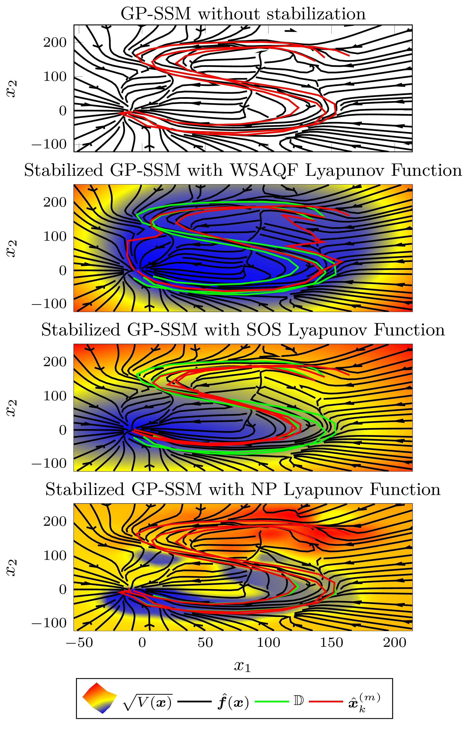
Figure 1: GP-SSM stabilized by different control Lyapunov functions together with the training data for the LASA S-shape movement.

$V(\bm{x}_{k})$	$\Delta_{\mathrm{rep}}$ S shape	$\Delta_{\mathrm{rep}}$ all 24	$\bar{t}_{\mathrm{train}}$	$\bar{t}_{\mathrm{test}}$
WSAQF	14276	2377	0.7468$s$	0.0101$s$
SOS	6107	1819.8	0.4655$s$	0.0083$s$
Our method ”NP”	280.99	415.6	2.9536$s$	0.0056$s$

Table 1: Reproduction error and average computation times for Lyapunov function training and stabilizing control computation.

4.3 Discussion

The simulations clearly show that the nonparametric control Lyapunov function in combination with a noise-free GP-SSM allows the precise reproduction of observed training data. Since existing approaches such as SOS or WSAQF are limited by the number of used parameters, not all training samples satisfy the stability conditions. Therefore, the stabilizing control $\bm{u}(\bm{x})$ computed based on the SOS and WSAQF control Lyapunov functions can cause a deviation from the observed trajectories. In contrast, our nonparametric approach adapts its flexibility to the data. Although the nonparametric Lyapunov function exhibits local minima, this does not cause an increasing Lyapunov function along trajectories. Instead, a local minimum leads to discrete-time dynamics, which can have large differences between consecutive states, since the system must move from the local minimum to a state with smaller Lyapunov function within a single time step. Moreover, the nonparametric Lyapunov function approach relies on a precise nominal model: when the nominal model is too imprecise such that the nominal trajectories deviate significantly from the training data, the approximate infinite horizon cost $V_{\infty}(\cdot)$ is almost zero such that the quadratic stage cost $l(\cdot)$ dominates. Therefore, trajectories do generally not converge to training data which would be necessary for a risk-sensitive behavior with awareness of the sparsity of data. However, this does not affect stability of the obtained model and could be overcome by employing the approach proposed in (Pöhler et al., 2019). Furthermore, the dominance of the quadratic cost $l(\cdot)$ exhibits also advantages regarding the computation time of the optimal controls $\bm{u}^{*}(\bm{x})$ such that the nonparametric Lyapunov function is the fastest on average (see Table 1).

5 Conclusion

In this paper, we develop a novel approach for learning a fully nonparametric, asymptotically stable model, which is capable of precisely reproducing observed data. We show that deterministic training data can be learned exactly with GP-SSMs, and employ a nonparametric control Lyapunov function learned from the data to stabilize the nominal GP-SSM without modifying the nominal model at training points. In a comparison to existing GP-SSM stabilization approaches on a real world dataset the superior flexibility and precision of the nonparametric control Lyapunov function is demonstrated. In order to extend the applicability of the approach to systems with noisy data, we will modify the approach in future work, such that stochastic stability conditions can be considered for learning the nonparametric Lyapunov function.

References

- Figueroa and Billard (2018) Figueroa, N. and Billard, A. (2018). A Physically-Consistent Bayesian Non-Parametric Mixture Model for Dynamical System Learning. In Proceedings of the Conference on Robot Learning, volume 87, 927–946.
- Khansari-Zadeh and Billard (2011) Khansari-Zadeh, S.M. and Billard, A. (2011). Learning stable nonlinear dynamical systems with Gaussian mixture models. IEEE Transactions on Robotics, 27(5), 943–957.
- Lacy and Bernstein (2003) Lacy, S.L. and Bernstein, D.S. (2003). Subspace identification with guaranteed stability using constrained optimization. IEEE Transactions on Automatic Control, 48(7), 1259–1263.
- Lederer and Hirche (2019) Lederer, A. and Hirche, S. (2019). Local Asymptotic Stability Analysis and Region of Attraction Estimation with Gaussian Processes. In Proceedings of the IEEE Conference on Decision and Control.
- Lemme et al. (2014) Lemme, A., Neumann, K., Reinhart, R., and Steil, J. (2014). Neural Learning of Vector Fields for Encoding Stable Dynamical Systems. Neurocomputing, 141, 3–14.
- Mohammad Khansari-Zadeh and Billard (2014) Mohammad Khansari-Zadeh, S. and Billard, A. (2014). Learning control Lyapunov function to ensure stability of dynamical system-based robot reaching motions. Robotics and Autonomous Systems, 62(6), 752–765.
- Neumann et al. (2013) Neumann, K., Lemme, A., and Steil, J.J. (2013). Neural learning of stable dynamical systems based on data-driven Lyapunov candidates. In IEEE International Conference on Intelligent Robots and Systems, 1216–1222. IEEE.
- Papachristodoulou and Prajna (2005) Papachristodoulou, A. and Prajna, S. (2005). A Tutorial on Sum of Squares Techniques for Systems Analysis. In Proceedings of the American Control Conference, 2686–2700.
- Pentland and Liu (1999) Pentland, A. and Liu, A. (1999). Modeling and prediction of human behavior. Neural Computation, 11(1), 229–242.
- Pöhler et al. (2019) Pöhler, L., Umlauft, J., and Hirche, S. (2019). Uncertainty-based Human Motion Tracking with Stable Gaussian Process State Space Models. IFAC-PapersOnLine, 51(34), 8–14.
- Rasmussen and Williams (2006) Rasmussen, C.E. and Williams, C.K.I. (2006). Gaussian Processes for Machine Learning. The MIT Press, Cambridge, MA.
- Steinwart (2001) Steinwart, I. (2001). On the Influence of the Kernel on the Consistency of Support Vector Machines. Journal of Machine Learning Research, 2, 67–93.
- Umlauft et al. (2017) Umlauft, J., Lederer, A., and Hirche, S. (2017). Learning Stable Gaussian Process State Space Models. In Proceedings of the American Control Conference, 1499–1504.
- Umlauft et al. (2018) Umlauft, J., Pöhler, L., and Hirche, S. (2018). An Uncertainty-Based Control Lyapunov Approach for Control-Affine Systems Modeled by Gaussian Process. IEEE Control Systems Letters, 2(3), 483–488.