Cityscapes 3D: Dataset and Benchmark for 9 DoF Vehicle Detection

Abstract

Detecting vehicles and representing their position and orientation in the three dimensional space is a key technology for autonomous driving. Recently, methods for 3D vehicle detection solely based on monocular RGB images gained popularity. In order to facilitate this task as well as to compare and drive state-of-the-art methods, several new datasets and benchmarks have been published. Ground truth annotations of vehicles are usually obtained using lidar point clouds, which often induces errors due to imperfect calibration or synchronization between both sensors.

To this end, we propose Cityscapes 3D, extending the original Cityscapes dataset with 3D bounding box annotations for all types of vehicles. In contrast to existing datasets, our 3D annotations were labeled using stereo RGB images only and capture all nine degrees of freedom. This leads to a pixel-accurate reprojection in the RGB image and a higher range of annotations compared to lidar-based approaches. In order to ease multitask learning, we provide a pairing of 2D instance segments with 3D bounding boxes. In addition, we complement the Cityscapes benchmark suite with 3D vehicle detection based on the new annotations as well as metrics presented in this work. Dataset and benchmark are available online.

1 Introduction

3D object detection is commonly approached by using lidar or radar sensors as they have exceptional physical properties for this task. More recently, vision-based methods have been proposed that detect objects in 3D solely relying on a single monocular RGB image [4, 17, 2, 21, 19, 18, 20]. These methods gained more and more interest as cameras are more prevalent than laser scanners or radars and allow for a finer-grained classification. Furthermore, they can be used as a redundant sensor in safety-critical applications such as autonomous driving. As no explicit 3D information is encoded in RGB images, accurate depth prediction is more challenging compared to lidar-based methods. This results in a significant gap in detection performance, which becomes evident via benchmarks that feature both modalities, e.g. KITTI (best lidar: $79.71\text{\,}\mathrm{\char 37\relax}$ [28], best monocular: $10.74\text{\,}\mathrm{\char 37\relax}$ [20]; 3D Average Precision (AP) for category Car) or nuScenes (best lidar $0.484$ [29], best monocular: $0.384$ [26]; nuScenes Detection Score).

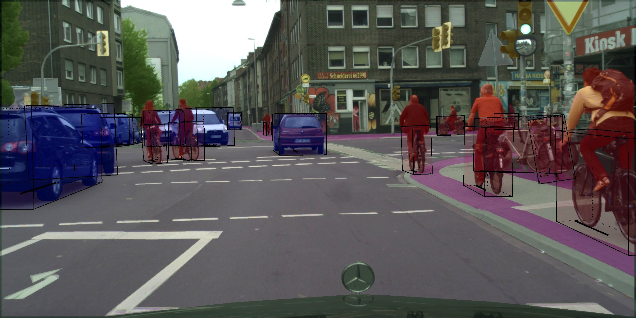
Figure 1: Example image with 3D bounding boxes for vehicles. The box annotations feature a full 3D orientation including yaw, pitch and roll labels.

To facilitate further research on monocular 3D object detection, we provide high quality 3D bounding box annotations of all types of vehicles for the Cityscapes dataset [8], which is one of the most popular datasets for semantic, instance, and panoptic segmentation. Based on these annotations, we offer a benchmark for 3D vehicle detection such that researchers can easily compare novel approaches with the state-of-the-art. Dataset and benchmark complement [8] and will also allow for future research, e.g. joint 3D detection and instance segmentation. To this end, we ensured consistency with the existing annotations and provide matches of 2D instance ground truth masks with the new 3D bounding box annotations.

In contrast to existing 3D object detection datasets and benchmarks, Cityscapes 3D is especially tailored for monocular 3D objection detection, due to three major design choices.

First, ground truth annotations are obtained using stereo RGB imagery only, which overcomes limitations of other datasets. Related real-world datasets, e.g. [7, 12, 6, 1], commonly rely on lidar point clouds for 3D bounding box annotation. This approach either requires high efforts regarding sensor setup, calibration and synchronization or suffers from drawbacks due to mismatches between both sensors, c.f. Fig. 2. These effects are most prominent in case of fast moving objects close to the ego-vehicle, i.e. exactly those objects that are highly relevant for self-driving cars.

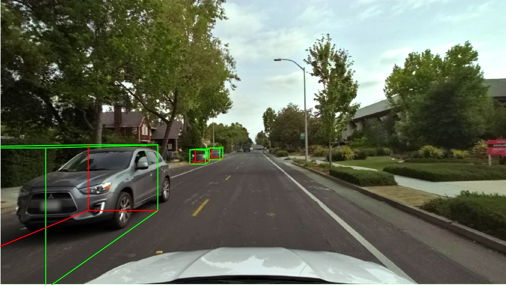
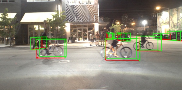
Figure 2: Examples of annotation artifacts due to lidar synchronization errors (top [16], bottom [7]).

Second, we provide full 3D orientation annotations including yaw, pitch, and roll angles to cover all nine degrees of freedom of a rigid object (position, extent, and orientation). As slanted roads occur in real-world scenes, such a representation is crucial to precisely describe and recognize vehicles in all constellations, c.f. Fig. 3.

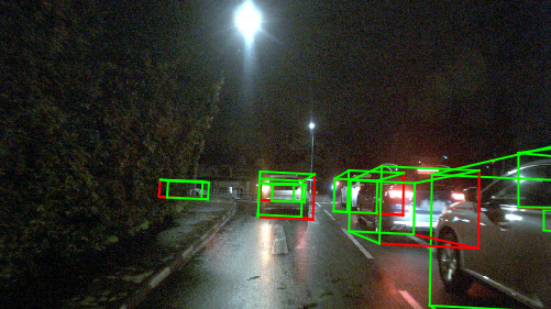
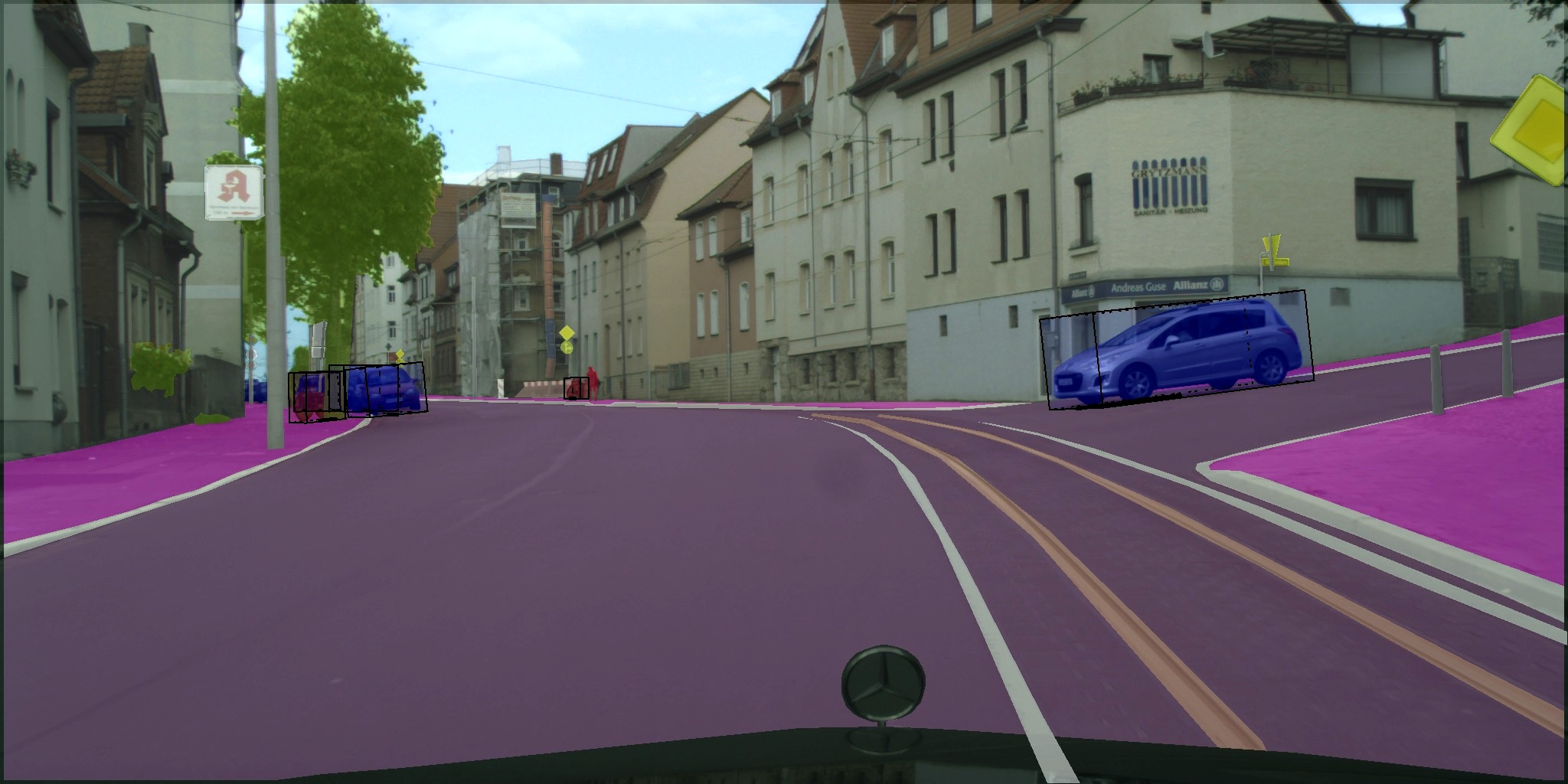
Figure 3: Top: Imprecise 3D box reprojections in [6] due to missing pitch and roll annotations. Bottom: Example for a car crossing from a steep street in Cityscapes 3D with pitch $>0$.

Third, the fundamental difference between lidar and RGB data as an input modality for 3D object detection is not sufficiently addressed in the current benchmark methodologies. While precise depth information is inherently included in lidar data, accurate depth estimation from monocular images is a challenging task. However, current benchmarks and their employed metrics are primarily designed for lidar-based approaches and often use the 3D Intersection over Union (IoU) metric with a high threshold. Doing so effectively requires centimeter accuracy, which can barely be achieved by vision-based approaches for distant objects and leads to a significant drop in accuracy compared to lidar-based methods. We therefore introduce novel metrics to assess the performance of monocular 3D object detection. Notably, the proposed metrics explicitly evaluate the performance depending on the distance of the object to the ego-vehicle.

2 Related Work

Table 1: Overview on datasets for autonomous driving featuring image-based vehicle recognition via 2D instance segmentation or 3D bounding box detection. Cityscapes 3D is the only dataset based on real-world data that supports both tasks with paired 2D instance segmentation masks and 3D bounding boxes. Furthermore, Cityscapes 3D was labeled using stereo images only, overcoming shortcomings due to calibration and synchronization issues.

		Annotations
Name	Resolution	Instance Masks	3D Boxes	3D Based on	Paired	3D Benchmark
Cityscapes 3D + [8]	$2.1\text{\,}\mathrm{M}\mathrm{P}$	✓	✓	stereo	✓	✓
A*3D [23]	$3.1\text{\,}\mathrm{M}\mathrm{P}$	✗	✓	lidar	✗	✗
A2D2 [13]	$2.3\text{\,}\mathrm{M}\mathrm{P}$	✓	✓	lidar	✗	✗
ApolloScape [15]	$9.2\text{\,}\mathrm{M}\mathrm{P}$	✓	✓	lidar	✗	✓
Argoverse [7]	$5.1\text{\,}\mathrm{M}\mathrm{P}$	✗	✓	lidar	✗	closed
BDD100k [30]	$0.9\text{\,}\mathrm{M}\mathrm{P}$	✓	✗	–	✗	✗
Boxy [3]	$5.1\text{\,}\mathrm{M}\mathrm{P}$	✗	trapezoid	monocular	✗	✓
KITTI [12]	$0.5\text{\,}\mathrm{M}\mathrm{P}$	✓	✓	lidar	✗	✓
Lyft [16]	$1.3$ & $2.1\text{\,}\mathrm{M}\mathrm{P}$	✗	✓	lidar	✗	closed
Mapillary Vistas [22]	various	✓	✗	–	✗	✗
nuScenes [6]	$1.4\text{\,}\mathrm{M}\mathrm{P}$	✓,	✓	lidar	✗	✓
Waymo Open [1]	$2.5\text{\,}\mathrm{M}\mathrm{P}$	✗	✓	lidar	✗	✓
Synscapes [27]	$2.1\text{\,}\mathrm{M}\mathrm{P}$	✓	✓	synthetic	✓	✗
Synthia [25]	$0.9$ & $2.1\text{\,}\mathrm{M}\mathrm{P}$	✓	✓	synthetic	✓	✗
VIPER [24]	$2.1\text{\,}\mathrm{M}\mathrm{P}$	✓	✓	synthetic	✓	✗
Virtual KITTI 2 [11, 5]	$0.5\text{\,}\mathrm{M}\mathrm{P}$	✓	✓	synthetic	✓	✗
only some instances per semantic class in an image
only a subset of the images in the dataset
to be released

There are multiple datasets available that address different problems in perception for autonomous driving such as object detection or instance segmentation. An overview of current datasets for autonomous driving with a focus on segmenting and detecting all types of vehicles is given in Table 1.

These datasets provide a wide range of driving scenarios as they were recorded at various locations all over the world; e.g. in the US [7, 6, 1], Singapore [6, 23], China [15], or Germany [12, 8]. Mapillary Vistas [22] even contains images from 6 continents. While only half of the datasets include instance masks as ground truth annotations, nearly all provide 3D bounding boxes. While instance masks are often only available for a subset of the dataset, 3D bounding boxes are usually provided for the whole dataset.

The majority of 3D bounding box annotations is labeled using lidar data [1, 6, 16]. However, using lidar data is vulnerable to calibration and synchronization errors, c.f. Fig. 2 which may result in imprecise reprojections into the RGB images. The only exceptions are Boxy [3], which was annotated in the image domain to obtain 3D ground truth data, and ApolloScapes [15] where CAD models were used for ground truth generation. In this work, we build our annotation workflow on top of stereo image pairs in order to obtain accurate and well-aligned 3D bounding boxes.

As shown previously, bounding boxes that are generated from instance segmentation masks help to boost amodal 2D object detection [10] and can be beneficial for 3D object detection from monocular RGB images as well [18, 21]. Furthermore, such paired annotations, i.e. direct mappings between instance masks and 3D bounding boxes, ease multitask learning. However, Cityscapes 3D is the only dataset out of those in Table 1 that provides such a mapping between the two modalities for all annotated images.

In addition to real-world datasets, there exist several synthetic ones such as [27, 25, 24, 5]. By design, synthetic datasets include high quality labels for all types of annotations. However, these datasets suffer from a domain gap towards real-world scenes, which makes them less suitable for benchmark purposes.

3 Labeling Process

Recent datasets for autonomous driving often include 3D bounding box annotations that were mainly labeled in lidar point clouds, as can be seen in Table 1. Using these annotations to benchmark monocular 3D bounding box detection methods proves difficult as the correctness of the projection into corresponding RGB images relies heavily on correct cross-sensor calibration and synchronization. This circumstance is highlighted in Fig. 2.

In contrast, for Cityscapes 3D we aim at monocular 3D bounding box detection. Thus, all 3D bounding box annotations are exclusively labeled using the stereo camera, preventing issues with calibration and synchronization. To this end, we exploit stereo data from [8] that was generated using semi-global matching (SGM) [14] with on-site calibration prior to each recording session. The main challenge of labeling 3D bounding boxes in RGB images is the indistinctness between depth and size of 3D objects in images. Objects of vastly different size may look equally large in images when placed at appropriate distances. To overcome this issue, we employed two techniques during our annotation workflow, i.e. stereo point clouds and size prototypes.

Figure 4: Workflow of creating the 3D bounding box annotations given the existing instance polygons and stereo measurements.

The labeling process of Cityscapes 3D is schematically visualized in Fig. 4. We initialize our workflow with the vehicle instances as annotated in [8]. For each vehicle, the occlusion as well as the truncation of the shown object are manually estimated in $10\text{\,}\mathrm{\char 37\relax}$ intervals. Vehicles that are more than $80\text{\,}\mathrm{\char 37\relax}$ occluded or $60\text{\,}\mathrm{\char 37\relax}$ truncated are filtered out, i.e. they are not annotated with a 3D bounding box and also set to ignore in the Cityscapes 3D benchmark, c.f. Section 5. For all remaining vehicle instances, the labeler selects a finer-grained vehicle type, c.f. Table 2 for a list of available categories. The selected category is then used as size prototype, i.e. an initial size as well as an initial orientation of the 3D bounding box annotation are assigned. The initial position of the 3D bounding box is then determined by the stereo measurements contained in the instance-level annotation polygon from [8]. Initial dimensions paired with an initial position estimate prevent errors caused by the trade-off between object size and depth of three dimensional objects in images. Preliminary experiments showed that this procedure significantly improves the annotation quality and speed compared with labeling from scratch.

Table 2: Size prototypes used for initial dimensions of the 3D bounding box annotations during labeling.

	Dimensions [$\mathrm{m}$]
Prototype Name	Height	Width	Length
Mini Car	1.45	1.65	2.70
Small Car	1.45	1.65	4.00
Compact Car	1.45	1.80	4.30
Sedan	1.45	1.81	4.70
Station Wagon	1.50	1.85	4.90
Box Wagon	1.80	1.80	4.35
Sports Utility Vehicle	1.70	1.90	4.70
Pick-Up	1.80	1.92	5.30
Sports Car	1.30	1.81	4.13
Small Van	1.90	1.90	5.40
Large Van	2.60	1.85	6.50
Caravan	3.00	2.20	7.20
Mini Truck	3.00	2.20	7.00
Small Truck	3.45	2.32	7.95
Medium Truck	4.00	2.50	12.00
Large Truck	4.00	2.55	6.80
Truck Trailer	4.00	2.55	13.60
Urban Bus (Solo)	3.10	2.55	12.00
Urban Bus (Front)	3.10	2.55	7.40
Urban Bus (Back)	3.10	2.55	7.40
Coach Bus	3.80	2.55	14.00
Bicycle	1.10	0.42	1.80
Motorbike	1.12	0.80	2.20

The labeler is subsequently asked to fine-tune orientation, position and dimensions of the 3D bounding box in a bird’s-eye view projection of the stereo measurements while checking the plausibility of the annotation in the RGB image. The RGB image information enables the labeling of full 3D orientation information (yaw, pitch, roll). An example of an RGB image with corresponding bird’s-eye view is shown in Fig. 5.

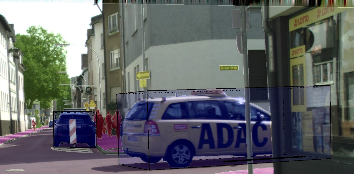
(a) 3D bounding box annotation projected into the RGB image

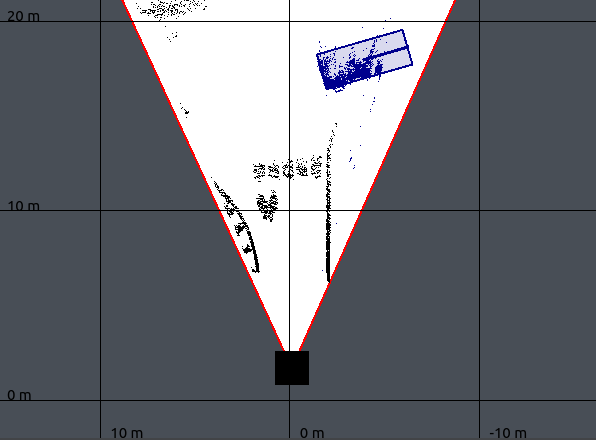
(b) Corresponding bird’s-eye view labeling aid

Figure 5: Example for bird’s-eye view labeling aid. 3D bounding box annotations and the stereo point cloud filtered for vehicles and markings are shown from a top view perspective of the scene.

In case of a vehicle with several moving parts, e.g. an articulated bus, multiple 3D bounding boxes were annotated to cover each movable part. Fig. 6 depicts an example of a bended articulated bus. As in some situations, e.g. very crowded scenes, it is not possible to identify single object instances, the whole object group is marked as such and ignored during evaluation, c.f. Section 5. An example for a crowded scene is shown in Fig. 7.

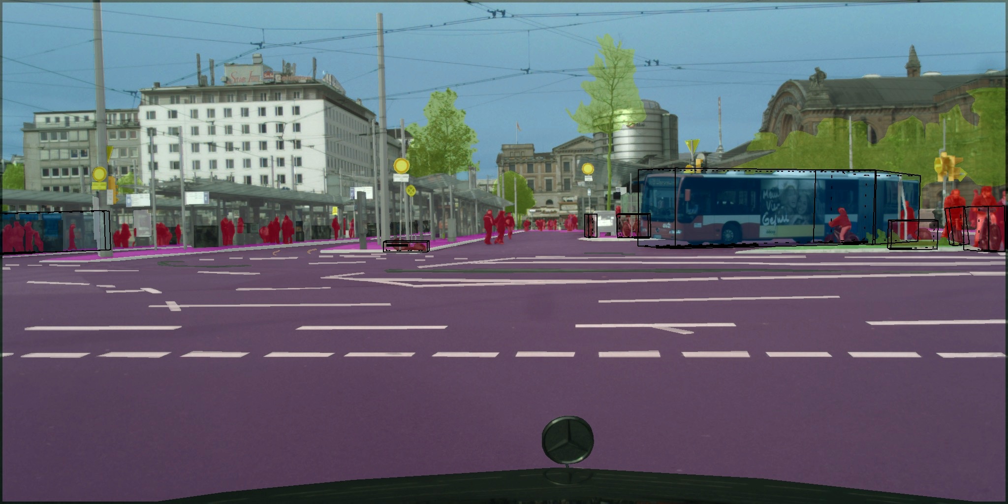
Figure 6: An articulated bus with two distinct 3D bounding boxes.

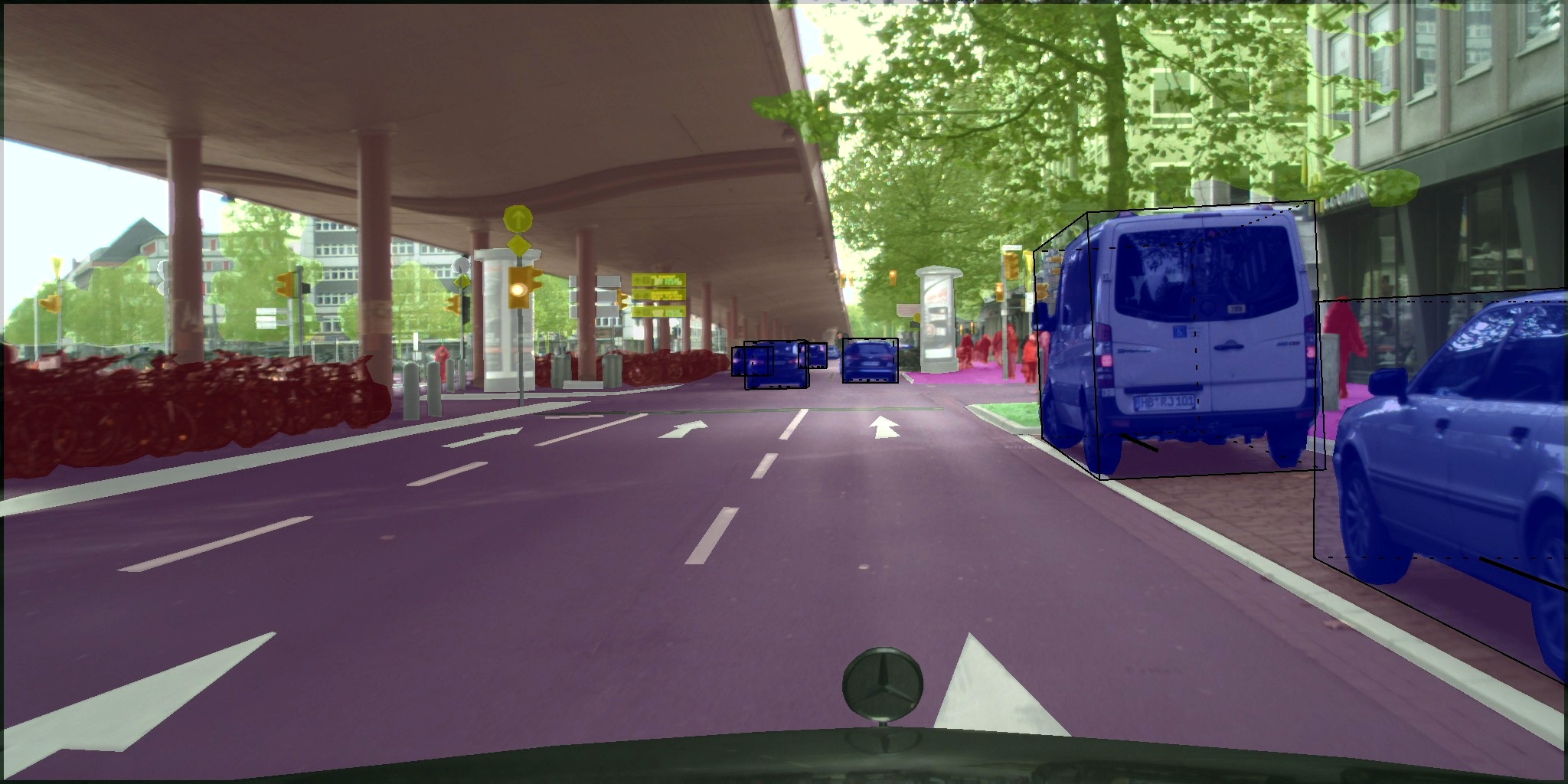
Figure 7: Crowded traffic scene. No single bicycle can be identified. Hence, the whole region is set to ignore and overlapping detections will not be considered during the evaluation.

In addition to the 3D bounding box annotations, the dataset contains the mapping between instance segments and 3D bounding box annotations. Furthermore, we provide the aforementioned metadata including occlusion, truncation, and selected size prototype per each 3D box.

4 Dataset Analysis

Cityscapes 3D extends the original dataset [8], which focuses on semantic and instance segmentation. The Cityscapes dataset contains $5000$ images split into $2975$ images for training, $500$ images for validation, and $1525$ images for testing.

Our 3D bounding box annotations cover all $8$ semantic classes in the vehicle category of the Cityscapes dataset, i.e. car, truck, bus, on rails, motorcycle, bicycle, caravan, and trailer. Analogously to [8], we ignore caravan and trailer during evaluation. Compared to other 3D detection datasets, Cityscapes 3D has a high object density, which in turn indicates complex scenes and hence renders successful detection a challenging task, c.f. Table 3. Furthermore, due to the labeling process with size prototypes as presented in Section 3, we also enriched Cityscapes with information about the fine grained types of a vehicle instances, c.f. Fig. 8 for a statistical analysis.

Table 3: Average number of 3D annotations per image for the train and val sets of different datasets. The column TBT combines truck, bus, and train. Cityscapes 3D has a high object density across all classes.

	Car	TBT	Bicycle	Motorbike
ApolloScapes	11.6	0.0	0.0	0.0
Argoverse	4.1	0.3	0.1	0.001
KITTI	4.2	0.2	0.0	0.0
nuScenes	3.0	0.6	0.07	0.07
Waymo	3.2	0.0	0.04	0.0
Cityscapes 3D	6.4	0.2	1.2	0.2

Figure 8: Number of different vehicle types in Cityscapes 3D train and val.

Figure 9: Distribution of distance of all objects for state-of-the-art datasets on train and val.

In contrast to the majority of existing 3D object detection datasets, we use stereo point clouds to annotate 3D bounding boxes instead of lidar measurements. This allows us to overcome issues due to the sparsity of lidar measurements, especially for distant objects. As a result, the distribution of vehicles over the distance to the camera has a long tail at far distances as illustrated in Fig. 9.

To estimate the quality of our 3D bounding box annotations, we compare the results of our labeling approach with perfect ground truth from synthetic data. To this end, we used our annotation tool and workflow to relabel $20$ images from the Synscapes dataset [27], which was designed to align well with Cityscapes. The human-labeled annotations are subsequently compared to the perfect Synscapes ground truth, see Fig. 10. The analysis shows an average error in the annotated yaw angle of below $2.1\text{\,}\mathrm{\SIUnitSymbolDegree}$ as well as an average center position error of below $1\text{\,}\mathrm{m}$ for all distance levels. Without the bird’s-eye view labeling aid, the average errors in both categories are significantly higher and increase with the distance of the objects, confirming the effectiveness of our annotation scheme.

Figure 10: Labeling quality evaluation of $20$ relabeled images in the Synscapes [27] dataset using the Cityscapes 3D labeling workflow. Labelers were asked to label 3D bounding boxes w/ and w/o the stereo bird’s-eye view. Annotation quality is compared to the synthetic ground truth.

5 Benchmark Metrics

To evaluate the performance of an RGB-based detection model in the Cityscapes 3D benchmark, we propose several metrics in the following that individually assess recognition performance in terms of 2D and 3D detection and localization. All metrics are then combined into a single detection score per class. The mean over all classes is denoted as mean detection score (mDS) and is used for ranking the approaches within the benchmark. As described in Section 4, the $8$ vehicle classes of the Cityscapes instance segmentation benchmark are evaluated taking ignore regions into account, c.f. Section 3. The circumscribing 2D bounding box of an ignore region defines this region as ignore and overlapping detections within these regions will not count as false positive.

The detection performance in popular benchmarks is commonly evaluated either distance independent or only for very coarse distance intervals. KITTI [12] and nuScenes [6] use the same detection thresholds for all distances and hence count all objects equally, irrespective of their distance to the camera. The metrics of Waymo Open [1] cluster objects in three rather coarse ranges from $0$ to $35\text{\,}\mathrm{m}$, from $35$ to $50\text{\,}\mathrm{m}$ and from $50\text{\,}\mathrm{m}$ to inf. In contrast, we aim for a more detailed depth-dependent performance analysis.

As our benchmark focuses on detecting 3D bounding boxes from monocular RGB images, we employ a metric consisting of two factors. The first factor is the 2D Average Precision (AP) metric, which is well-known and the standard metric to assess 2D bounding box detection performance.

As second factor, we summarize three-dimensional core properties, i.e. center position in 3D space, orientation, and size. These aspects are evaluated individually using Depth-Dependent True Positive (DDTP) metrics. These metrics are only calculated for true positive detections and their corresponding ground truth counterpart. The 3D ground truth annotations are binned based on their distance to the camera such that we can obtain a depth-dependent analysis. For each bin and DDTP metric, we compute the average score in terms of accuracy of the underlying 3D property. Eventually, the DDTP value is determined as the average over all distance bins.

This two-factor approach allows to distinguish between semantics and geometry. For example, a detection with an accurate projection into the RGB image but with a poor distance estimation counts as a true positive in the 2D AP computation and at the same time lowers the DDTP metric that assesses the quality of 3D localization. In contrast, the metric definitions of e.g. KITTI [12] or nuScenes [6] do not provide such a fine analysis and lead to an overall decreased model accuracy.

In the following $X_{\text{max}}$ is defined as the maximum detection radius up to which the object detection performance shall be analyzed. A bin $D(s,c)$ denotes the set of pairs of detections $d$ and ground truth objects $g$ within the depth range $[s,s+\delta_{s})$ and a minimum detection confidence of $c$. $N$ is the cardinality of $D(s,c)$. We set the maximum detection depth $X_{\text{max}}=$100\text{\,}\mathrm{m}$$ as $90\text{\,}\mathrm{\char 37\relax}$ of all annotated objects are within $100\text{\,}\mathrm{m}$ distance to the ego-vehicle. We choose $\delta_{s}=$5\text{\,}\mathrm{m}$$ for the bin size.

5.1 2D Average Precision (AP)

We use standard Average Precision (AP) [9] for assessing the 2D detection performance based on 2D bounding boxes. The 2D bounding box of both, ground truth and predicted 3D box, is defined as the circumscribing rectangle of all 8 vertices of the 3D box projected into the image. Matching is conducted in the 2D space and we require an IoU of $0.7$ between ground truth and detection to accept the detection as true positive.

Detections for which at least $70\text{\,}\mathrm{\char 37\relax}$ of the predicted 2D bounding box covers any ignore region will be discarded and not included in the evaluation. Ignore regions typically contain groups of objects that cannot be visually separated or objects with high occlusion or truncation, c.f. Section 3.

Overall, AP is defined as

$$\text{AP }=\int p(r)\mathrm{d}r$$ (1)

with $p(r)$ being the precision value for recall $r$.

5.2 Depth-Dependent Average Precision

We calculate standard AP for all objects within the range $[s,s+\delta_{s})$. To assign a depth value to an object, we take the ground truth depth for true positive and false negative detections and the predicted depth for false positives.

5.3 Depth-Dependent True Positive Metrics

We calculate several depth-dependent true positive metrics, i.e. BEV Center Distance, Yaw Similarity, Pitch-Roll Similarity, and Size Similarity. The depth of the ground truth box is used to determine the applicable interval $[s,s+\delta_{s})$. In contrast to the regular 2D AP score Eq. 1, we use a fixed confidence threshold for the depth-dependent true positive metrics. The threshold $c_{w}$ is defined as

$$c_{w}=\underset{c\in[0,1]}{\operatorname{arg\,max}}p(c)r(c)$$ (2)

with $p(c)$ and $r(c)$ denoting the precision and the recall for score $c$. Fixing the confidence to $c_{w}$ is motivated by the observation that most perception systems use fixed confidence thresholds to limit the number of detected objects and hence requirements and bandwidths for downstream applications. By this definition we allow for an assessment of the quality of each model as is when deployed.

Center Distance

Bird’s-Eye View Center Distance is defined as the normalized integral of the depth-dependent distance up to the maximum depth of interest $X_{\text{max}}$, i.e.

$$\text{BEVCD}=1-\frac{1}{X_{\text{max}}^{2}}\int_{0}^{X_{\text{max}}}k(s)\mathrm{d}s$$ (3)

with

$$k(s)=\frac{1}{N}\sum_{d,g\in D(s,c_{w})}\min\left(X_{\text{max}},\sqrt{\sum_{i\in\{x,y\}}(d_{i}-g_{i})^{2}}\right).$$ (4)

As the maximal center distance is limited to $X_{\text{max}}$ the integral is scaled by the inverse of $X_{\text{max}}^{2}$ to obtain a value between $0$ and $1$.

Yaw Similarity

Following the same scheme, Yaw Similarity is inspired by [12] and is defined as

$$\text{YawSim}=\frac{1}{X_{\text{max}}}\int_{0}^{X_{\text{max}}}k(s)\mathrm{d}s$$ (5)

with

$$k(s)=\frac{1}{N}\sum_{d,g\in D(s,c_{w})}\frac{1+\cos{\left(\Delta_{\text{Yaw}}\right)}}{2}.$$ (6)

However, it is not required to scale by the squared value of $X_{\text{max}}$ as $\frac{1+\cos}{2}$ is limited between $0$ and $1$.

Pitch-Roll Similarity

Pitch-Roll Similarity is calculated analogously to Yaw Similarity but both pitch and roll orientation are combined since pitch and roll of a vehicle are not independent in realistic driving scenarios, i.e.

$$\text{PRSim}=\frac{1}{X_{\text{max}}}\int_{0}^{X_{\text{max}}}k(s)\mathrm{d}s$$ (7)

with

$$k(s)=\frac{1}{N}\sum_{d,g\in D(s,c_{w})}\frac{2+\cos{\left(\Delta_{\text{Pitch}}\right)}+\cos{\left(\Delta_{\text{Roll}}\right)}}{4}.$$ (8)

Size Similarity

Size Similarity assesses the 3D dimensions of the true positive detection and is defined as

$$\text{SizeSim}=\frac{1}{X_{\text{max}}}\int_{0}^{X_{\text{max}}}k(s)\mathrm{d}s$$ (9)

with

$$k(s)=\frac{1}{N}\sum_{d,g\in D(s,c_{w})}\prod_{x\in\{l,w,h\}}\min\left(\frac{d_{x}}{g_{x}},\frac{g_{x}}{d_{x}}\right)$$ (10)

with $l,w,h$ being length, width, and height of the corresponding 3D bounding box.

5.4 Detection Score

To combine all quality measures, we define the detection score per class as

$$\text{DS}=\text{AP}\times\frac{\text{BEVCD}+\text{YawSim}+\text{PRSim}+\text{SizeSim}}{4}.$$ (11)

By this definition, we enforce the 2D Average Precision to be an upper bound for the final detection score that can only be reached if all true positive bounding boxes are predicted perfectly. Furthermore, depth-dependent AP does not count to the overall detection score. Finally, the overall detection score mDS is calculated as the mean of all detection scores per class. mDS is consequently used for the benchmark ranking.

6 Conclusion

In this work, we presented a novel extension to the popular Cityscapes dataset, enriching the annotations with high quality 3D bounding boxes for vehicles. With this extension, we specifically aim at motivating progress in the important research area of monocular 3D object detection for autonomous driving.

We identified two major shortcomings of current state-of-the-art 3D object detection datasets and corresponding benchmarks that we address: (i) The majority of existing 3D object detection datasets relies on lidar point clouds for labeling. This introduces errors when projecting the annotations into RGB images if the cross-sensor calibration or synchronization are imperfect, thus hindering effective benchmarking of monocular 3D object detection methods. We address this issue by labeling the 3D box annotations using only RGB and stereo information, independent from multi-sensor calibration or synchronization. Hence, our 3D bounding box annotations are consistent in both, image and 3D space. (ii) Benchmark metrics of existing 3D object detection datasets are often relying on a minimum 3D IoU overlap for true positive detections which can be extremely hard to achieve with monocular detection methods, favoring lidar-based detection algorithms. Furthermore, state-of-the-art metrics are usually distance agnostic. However, especially in autonomous driving, the distance of objects to the ego-vehicle strongly correlates with the relevance of an object for the actual driving task. We address these findings by using 2D IoU thresholds for true positive detections, which adapts the matching optimally for monocular detection methods. Furthermore, we provide a set of novel, distance-dependent metrics that enable the benchmarking of monocular 3D object detection methods for autonomous driving.

References

- [1] Waymo open dataset: An autonomous driving dataset. https://waymo.com/open/, 2019.
- [2] Wentao Bao, Bin Xu, and Zhenzhong Chen. Monofenet: Monocular 3d object detection with feature enhancement networks. IEEE Transactions on Image Processing, 2019.
- [3] Karsten Behrendt. Boxy vehicle detection in large images. In ICCV, 2019.
- [4] Garrick Brazil and Xiaoming Liu. M3d-rpn: Monocular 3d region proposal network for object detection. In ICCV, 2019.
- [5] Yohann Cabon, Naila Murray, and Martin Humenberger. Virtual kitti 2. arXiv preprint arXiv:2001.10773, 2020.
- [6] Holger Caesar, Varun Bankiti, Alex H. Lang, Sourabh Vora, Venice Erin Liong, Qiang Xu, Anush Krishnan, Yu Pan, Giancarlo Baldan, and Oscar Beijbom. nuscenes: A multimodal dataset for autonomous driving. arXiv preprint arXiv:1903.11027, 2019.
- [7] Ming-Fang Chang, John W Lambert, Patsorn Sangkloy, Jagjeet Singh, Slawomir Bak, Andrew Hartnett, De Wang, Peter Carr, Simon Lucey, Deva Ramanan, and James Hays. Argoverse: 3d tracking and forecasting with rich maps. In CVPR, 2019.
- [8] Marius Cordts, Mohamed Omran, Sebastian Ramos, Timo Rehfeld, Markus Enzweiler, Rodrigo Benenson, Uwe Franke, Stefan Roth, and Bernt Schiele. The cityscapes dataset for semantic urban scene understanding. In CVPR, 2016.
- [9] Mark Everingham, Luc Van Gool, Christopher KI Williams, John Winn, and Andrew Zisserman. The pascal visual object classes (voc) challenge. International journal of computer vision, 88(2):303–338, 2010.
- [10] Nils Gählert, Niklas Hanselmann, Uwe Franke, and Joachim Denzler. Visibility guided nms: Efficient boosting of amodal object detection in crowded traffic scenes. In NeurIPS Workshops, 2019.
- [11] Adrien Gaidon, Qiao Wang, Yohann Cabon, and Eleonora Vig. Virtual worlds as proxy for multi-object tracking analysis. In CVPR, 2016.
- [12] Andreas Geiger, Philip Lenz, and Raquel Urtasun. Are we ready for autonomous driving? the kitti vision benchmark suite. In CVPR, 2012.
- [13] Jakob Geyer, Yohannes Kassahun, Mentar Mahmudi, Xavier Ricou, Rupesh Durgesh, Andrew S. Chung, Lorenz Hauswald, Viet Hoang Pham, Maximilian Mühlegg, Sebastian Dorn, Tiffany Fernandez, Martin Jänicke, Sudesh Mirashi, Chiragkumar Savani, Martin Sturm, Oleksandr Vorobiov, Martin Oelker, Sebastian Garreis, and Peter Schuberth. A2D2: AEV Autonomous Driving Dataset. http://www.a2d2.audi, 2019.
- [14] Heiko Hirschmüller. Stereo processing by semiglobal matching and mutual information. TPAMI, 30(2):328–341, 2007.
- [15] Xinyu Huang, Xinjing Cheng, Qichuan Geng, Binbin Cao, Dingfu Zhou, Peng Wang, Yuanqing Lin, and Ruigang Yang. The apolloscape dataset for autonomous driving. In CVPR Workshops, 2018.
- [16] R. Kesten, M. Usman, J. Houston, T. Pandya, K. Nadhamuni, A. Ferreira, M. Yuan, B. Low, A. Jain, P. Ondruska, S. Omari, S. Shah, A. Kulkarni, A. Kazakova, C. Tao, L. Platinsky, W. Jiang, and V. Shet. Lyft level 5 av dataset 2019. https://level5.lyft.com/dataset/, 2019.
- [17] Jason Ku, Alex D Pon, and Steven L Waslander. Monocular 3d object detection leveraging accurate proposals and shape reconstruction. In CVPR, 2019.
- [18] Buyu Li, Wanli Ouyang, Lu Sheng, Xingyu Zeng, and Xiaogang Wang. Gs3d: An efficient 3d object detection framework for autonomous driving. In CVPR, 2019.
- [19] Lijie Liu, Jiwen Lu, Chunjing Xu, Qi Tian, and Jie Zhou. Deep fitting degree scoring network for monocular 3d object detection. In CVPR, 2019.
- [20] Xinzhu Ma, Zhihui Wang, Haojie Li, Pengbo Zhang, Wanli Ouyang, and Xin Fan. Accurate monocular 3d object detection via color-embedded 3d reconstruction for autonomous driving. In ICCV, 2019.
- [21] Fabian Manhardt, Wadim Kehl, and Adrien Gaidon. Roi-10d: Monocular lifting of 2d detection to 6d pose and metric shape. In CVPR, 2019.
- [22] Gerhard Neuhold, Tobias Ollmann, Samuel Rota Bulo, and Peter Kontschieder. The mapillary vistas dataset for semantic understanding of street scenes. In ICCV, 2017.
- [23] Quang-Hieu Pham, Pierre Sevestre, Ramanpreet Singh Pahwa, Huijing Zhan, Chun Ho Pang, Yuda Chen, Armin Mustafa, Vijay Chandrasekhar, and Jie Lin. A* 3d dataset: Towards autonomous driving in challenging environments. arXiv preprint arXiv:1909.07541, 2019.
- [24] Stephan R Richter, Zeeshan Hayder, and Vladlen Koltun. Playing for benchmarks. In ICCV, 2017.
- [25] German Ros, Laura Sellart, Joanna Materzynska, David Vazquez, and Antonio M Lopez. The synthia dataset: A large collection of synthetic images for semantic segmentation of urban scenes. In CVPR, 2016.
- [26] Andrea Simonelli, Samuel Rota Bulo, Lorenzo Porzi, Manuel López-Antequera, and Peter Kontschieder. Disentangling monocular 3d object detection. In ICCV, 2019.
- [27] Magnus Wrenninge and Jonas Unger. Synscapes: A photorealistic synthetic dataset for street scene parsing. arXiv preprint arXiv:1810.08705, 2018.
- [28] Zetong Yang, Yanan Sun, Shu Liu, Xiaoyong Shen, and Jiaya Jia. Std: Sparse-to-dense 3d object detector for point cloud. In ICCV, 2019.
- [29] Yangyang Ye, Houjin Chen, Chi Zhang, Xiaoli Hao, and Zhaoxiang Zhang. Sarpnet: Shape attention regional proposal network for lidar-based 3d object detection. Neurocomputing, 379:53–63, 2020.
- [30] Fisher Yu, Wenqi Xian, Yingying Chen, Fangchen Liu, Mike Liao, Vashisht Madhavan, and Trevor Darrell. Bdd100k: A diverse driving video database with scalable annotation tooling. arXiv preprint arXiv:1805.04687, 2018.