PatchUp: A Feature-Space Block-Level Regularization Technique for Convolutional Neural Networks
Large capacity deep learning models are often prone to a high generalization gap when trained with a limited amount of labeled training data. A recent class of methods to address this problem uses various ways to construct a new training sample by mixing a pair (or more) of training samples. We propose PatchUp, a hidden state block-level regularization technique for Convolutional Neural Networks (CNNs), that is applied on selected contiguous blocks of feature maps from a random pair of samples. Our approach improves the robustness of CNN models against the manifold intrusion problem that may occur in other state-of-the-art mixing approaches. Moreover, since we are mixing the contiguous block of features in the hidden space, which has more dimensions than the input space, we obtain more diverse samples for training towards different dimensions. Our experiments on CIFAR10/100, SVHN, Tiny-ImageNet, and ImageNet using ResNet architectures including PreActResnet18/34, WRN-28-10, ResNet101/152 models show that PatchUp improves upon, or equals, the performance of current state-of-the-art regularizers for CNNs. We also show that PatchUp can provide a better generalization to deformed samples and is more robust against adversarial attacks.
1 Introduction
Deep Learning (DL), particularly deep Convolutional Neural Networks (CNNs) have achieved exceptional performance in many machine learning tasks, including object recognition (Krizhevsky, Sutskever, and Hinton 2012), image classification (Krizhevsky, Sutskever, and Hinton 2012; Ren et al. 2015; He et al. 2015), speech recognition (Hinton et al. 2012) and natural language understanding (Sutskever, Vinyals, and Le 2014; Vaswani et al. 2017). However, in a very deep and wide network, the network has a tendency to memorize the samples, which yields poor generalization for data outside of the training data distribution (Arpit et al. 2017; Goodfellow, Bengio, and Courville 2016). To address this issue, noisy computation is often employed during the training, making the model more robust against invariant samples and thus improving the generalization of the model (Achille and Soatto 2018). This idea is exploited in several state-of-the-art regularization techniques.
Such noisy computation based regularization techniques can be categorized into data-dependent and data-independent techniques (Guo, Mao, and Zhang 2018). Earlier work in this area has been more focused on the data-independent techniques such as Dropout (Srivastava et al. 2014), Variational Dropout (Gal and Ghahramani 2016) and ZoneOut (Krueger et al. 2016), Information Dropout (Achille and Soatto 2018), SpatialDropout (Tompson et al. 2014a), and DropBlock (Ghiasi, Lin, and Le 2018). Dropout performs well on fully connected layers (Srivastava et al. 2014). However, it is less effective on convolutional layers (Tompson et al. 2014b). One of the reasons for the lack of success of dropout on CNN layers is perhaps that the activation units in the convolutional layers are correlated, thus despite dropping some of the activation units, information can still flow through these layers. SpatialDropout (Tompson et al. 2014b) addresses this issue by dropping the entire feature map from a convolutional layer. DropBlock (Ghiasi, Lin, and Le 2018) further improves SpatialDropout by dropping random continuous feature blocks from feature maps instead of dropping the entire feature map in the convolutional layers.
Data-augmentation also is a data-dependent solution to improve the generalization of a model. Choosing the best augmentation policy is challenging. AutoAugment (Cubuk et al. 2019) finds the best augmentation policies using reinforcement learning with huge computation overhead. AugMix (Hendrycks et al. 2020) reduces this overhead by using stochasticity and diverse augmentations and adding a Jensen-Shannon Divergence consistency loss to training loss. Recent works show that data-dependent regularizers can achieve better generalization for CNN models. Mixup (Zhang et al. 2017), one such data-dependent regularizer, synthesizes additional training examples by interpolating random pairs of inputs , and their corresponding labels , as:
| (1) |
where is sampled from a Beta distribution such that and () is the new example. By using these types of synthetic samples, Mixup encourages the model to behave linearly in-between the training samples. The mixing coefficient in Mixup is sampled from a prior distribution. This may lead to the manifold intrusion problem (Guo, Mao, and Zhang 2018): the mixed synthetic example may collide (i.e. have the same value in the input space) with other examples in the training data, essentially leading to two training samples which have the same inputs but different targets. To overcome the manifold intrusion problem, MetaMixUp (Mai et al. 2019) used a meta-learning approach to learn with a lower possibility of causing such collisions. However, this meta-learning approach adds significant computation complexity. ManifoldMixup (Verma et al. 2019) attempts to avoid the manifold intrusion problem by interpolating the hidden states (instead of input states) of a randomly chosen layer at every training update. Recently, Puzzle Mix (Kim, Choo, and Song 2020) explicitly exploits an optimized masking strategy for the Input Mixup. It uses the saliency information and the underlying statistics of pair of images to avoid manifold intrusion problems at each batch training step. Puzzle Mix adds computation overhead at training time to find an optimal mask policy while improving the performance of the model in comparison to Mixup and ManifoldMixup.
Different from the interpolation-based regularizers discussed above, Cutout (DeVries and Taylor 2017) drops the contiguous regions from the image in the input space. This kind of noise encourages the network to learn the full context of the images instead of overfitting to the small set of visual features. CutMix (Yun et al. 2019) is another data-dependent regularization technique that cuts and fills rectangular shape parts from two randomly selected pairs in a mini-batch instead of interpolating two selected pairs completely. Applying CutMix at the input space improves the generalization of the CNN model by spreading the focus of the model across all places in the input instead of just a small region or a small set of intermediate activations. According to the CutMix paper, applying CutMix at the latent space, Feature CutMix, is not as effective as applying CutMix in the input space (Yun et al. 2019).
In this work, we introduce a feature-space block-level data-dependent regularization that operates in the hidden space by masking out contiguous blocks of the feature map of a random pair of samples, and then either mixes (Soft PatchUp) or swaps (Hard PatchUp) these selected contiguous blocks. Our regularization method does not incur significant computational overhead for CNNs during training. PatchUp improves the generalization of ResNet architectures on image classification task (on CIFAR-10, CIFAR-100, SVHN, and Tiny-ImageNet), deformed images classification, and against adversarial attacks. It also helps a CNN model to produce a wider variety of features in the residual blocks compared to other state-of-the-art regularization methods for CNNs such as Mixup, Cutout, CutMix, ManifoldMixup, and Puzzle Mix.
2 PatchUp
PatchUp is a hidden state block-level regularization technique that can be used after any convolutional layer in CNN models. Given a deep neural network where is the input, let be the -th convolutional layer. The network can be represented as where is the mapping from the input data to the hidden representation at layer and is the mapping from the hidden representation at layer to the output (Verma et al. 2019). In every training step, PatchUp applies block-level regularization at a randomly selected convolutional layer from a set of intermediate convolutional layers. appx.B gives a formal intuition for selecting randomly.
Binary Mask Creation
Once a convolutional layer is chosen, the next step is to create a binary mask (of the same size as the feature map in layer ) that will be used to PatchUp a pair of examples in the space of . The mask creation process is similar to that of DropBlock (Ghiasi, Lin, and Le 2018). The idea is to select contiguous blocks of features from the feature map that will be either mixed or swapped with the same features in another example. To do so, we first select a set of features that can be altered (mixed or swapped). This is done by using the hyper-parameter which decides the probability of altering a feature. When we alter a feature, we also alter a square block of features centered around that feature which is controlled by the side length of this square block, . Hence, the altering probabilities are readjusted using the following formula (Ghiasi, Lin, and Le 2018):
| (2) |
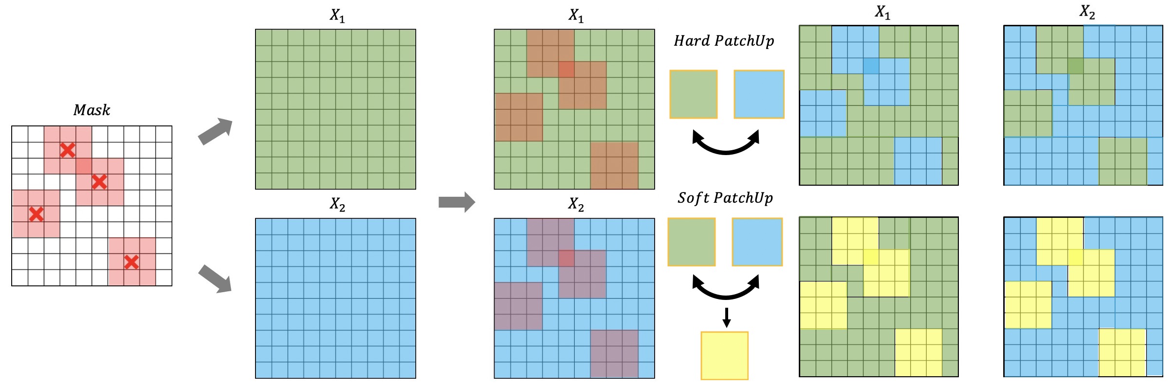
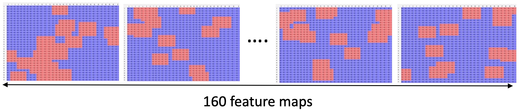
where the area of the feature map and block are the and , respectively, and the valid region to build the block is . For each feature in the feature map, we sample from . If the result of this sampling for feature is 0, then . If the result of this sampling for is 1, then the entire square region in the mask with the center and the width and height of the square of is set to 0. Note that these feature blocks to be altered can overlap which will result in more complex block structures than just squares. The block structures created are called patches. Fig.1 illustrates an example mask used by PatchUp. The mask has 1 for features outside the patches (which are not altered) and 0 for features inside the patches (which are altered). See Fig. 11 and 9 in Appendix for more details.
PatchUp Operation
Once the mask is created, we can use the mask to select patches from the feature maps and either swap these patches (Hard PatchUp) or mix them (Soft PatchUp).
Consider two samples and . The Hard PatchUp operation at layer is defined as follows:
| (3) |
where is known as the element-wise multiplication operation and is the binary mask described in section 2. To define Soft PatchUp operation, we first define the mixing operation for any two vectors and as follows:
| (4) |
where is the mixing coefficient. Thus, the Soft PatchUp operation at layer is defined as follows:
| (5) | ||||
where in the range of is sampled from a Beta distribution such that . controls the shape of the Beta distribution. Hence, it controls the strength of interpolation (Zhang et al. 2017). PatchUp operations are illustrated in Fig. 1 (see more details in Algorithm 1 in Appendix).
Learning Objective
After applying the PatchUp operation, the CNN model continues the forward pass from layer to the last layer in the model. The output of the model is used for the learning objective, including the loss minimization process and updating the model parameters accordingly. Consider the example pairs and . Let be the output of PatchUp after the -th layer. Mathematically, the CNN with PatchUp minimizes the following loss function:
| (6) | ||||
where is the fraction of the unchanged features from feature maps in and is the set of layers where PatchUp is applied randomly. is for Hard PatchUp and for Soft PatchUp.
is the target corresponding to the changed features. In the case of Hard PatchUp, and in the case of Soft PatchUp, . calculates the re-weighted target according to the interpolation policy for and . for Hard PatchUp and Soft PatchUp is defined as follows:
| (7) | |||
| (8) |
The PatchUp loss function has two terms where the first term is inspired from the CutMix loss function and the second term is inspired from the MixUp loss function (more detail in Appendix E).
PatchUp in Input Space
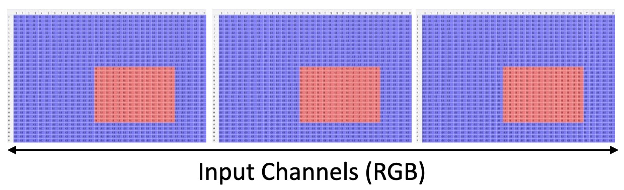
By setting , we can apply PatchUp to only the input space. When we apply PatchUp to the input space, only the Hard PatchUp operation is used, this is due to the reason that, as shown in (Yun et al. 2019), swapping in the input space provides better generalization compared to mixing. Furthermore, we select only one random rectangular patch in the input space (similar to CutMix) because the PatchUp binary mask is potentially too strong for the input space, which has only three channels, compared to hidden layers in which each layer can have a larger number of channels (more detail in section “4”).
3 Relation to Similar Methods

PatchUp Vs. ManifoldMixup:
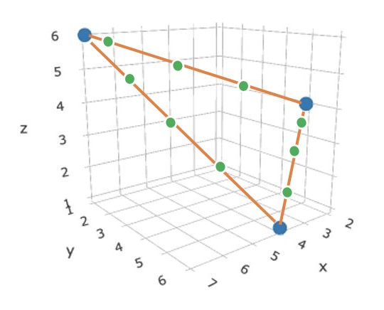
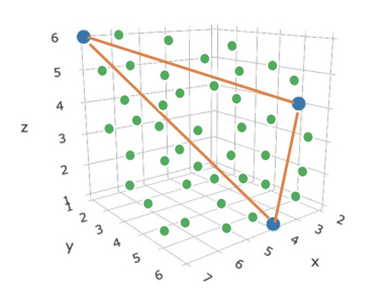
PatchUp and ManifoldMixup improve the generalization of a model by combining the latent representations of a pair of examples. ManifoldMixup linearly mixes two hidden representations using Equation 4. PatchUp uses a more complex approach ensuring that a more diverse subspace of the hidden space gets explored. To understand the behaviour and the limitation that exists in the ManifoldMixup, assume that we have a 3D hidden space representation as illustrated in Fig.3. It presents the possible combinations of hidden representations explored via ManifoldMixup and PatchUp. Blue dots represent real hidden representation samples. ManifoldMixup can produce new samples that lie directly on the orange lines which connect the blue point pairs due to its linear interpolation strategy. But, PatchUp can select various points in all dimensions, and can also select points extremely close to the orange lines. The proximity to the orange lines depends on the selected pairs and sampled from the beta distribution. Fig.3 is a simple diagrammatic description of how PatchUp constructs more diverse samples. Appx. C provides a mathematical and real experimental justification.
PatchUp Vs. CutMix:
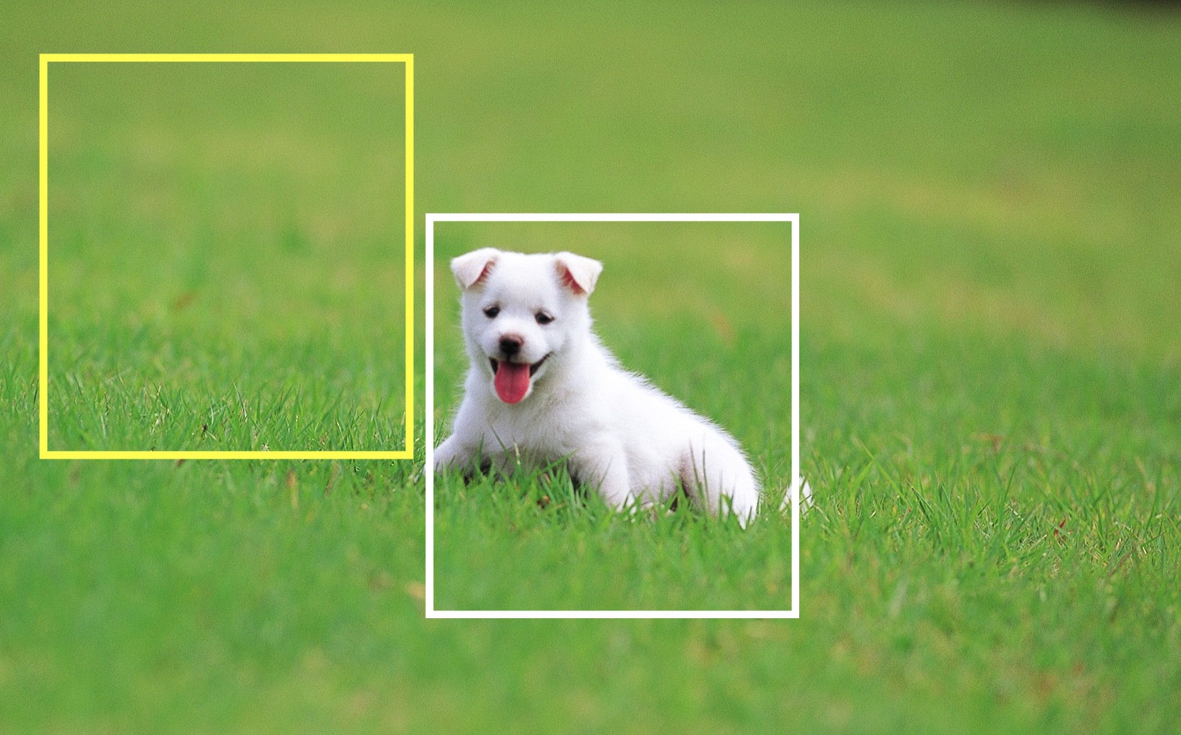
The CutMix cuts and fills the rectangular parts of the randomly selected pairs instead of using interpolation for creating a new sample in the input space. Therefore, CutMix has less potential for a manifold intrusion problem, however, CutMix may still suffer from a manifold intrusion problem. Fig.3 shows two samples with small portions that correspond to their labels. In this example, if only the parts within the yellow bounding boxes are swapped, then the label does not change. However, if the parts within the white bounding boxes are swapped, then the entire label is swapped. In both scenarios, CutMix only learns the interpolated target based on the fractions of the swapped part. In contrast, these scenarios are less likely to occur in PatchUp since it works in the hidden representation space most of the time. Another difference between CutMix and PatchUp is how the masks are created. PatchUp can create arbitrarily shaped masks while CutMix masks can only be rectangular. Fig.9 (appx.) shows an example of CutMix and PatchUp masks in input space and hidden representation space, respectively. CutMix is more effective than Feature-CutMix that applies CutMix in the latent space (Yun et al. 2019). The learning objective of PatchUp and the binary mask selection are both different from that of Feature-CutMix. Experiments
4 Experiments
This section presents the results of applying PatchUp to image classification tasks using various benchmark datasets such as CIFAR10, CIFfAR100 (Krizhevsky 2009), SVHN (the standard version with 73257 training samples) (Netzer et al. 2011), Tiny-ImageNet (Chrabaszcz, Loshchilov, and Hutter 2017), and with various benchmark architectures such as PreActResNet18/34 (He et al. 2016), and ResNet101, ResNet152, and WideResNet-28-10 (WRN-28-10) (Zagoruyko and Komodakis 2017)111The code is available: https://github.com/chandar-lab/PatchUp. We used the same set of base hyper-parameters for all the models for a thorough and fair comparison. The details of the experimental setup and the hyper-parameter tuning are given in appendix-E. We set to in PatchUp. PatchUp has , and as additional hyper-parameters. is the probability that PatchUp is performed for a given mini-batch. Based on our hyper-parameter tuning, Hard PatchUp yields the best performance with , , and as , , and , respectively. Soft PatchUp achieves the best performance with , , and as , , and , respectively.
Generalization on Image Classification
Table 2 shows the comparison of the generalization performance of PatchUp with six recently proposed mixing-based or feature-level methods on the CIFAR10/100, and SVHN datasets. Since Puzzle Mix clearly showed that both CutMix and Puzzle Mix perform better than AugMix (Kim, Choo, and Song 2020), we excluded it from our experiments. Tables 12 and 11 in appendix-I show test errors and NLLs. Our experiments show that PatchUp leads to a lower test error for all the models on CIFAR, SVHN, and Tiny-ImageNet with a large margin. Specifically, Soft PatchUp outperforms other methods on Tiny-ImageNet dataset using ResNet101/152, and WRN-28-10 followed by Hard PatchUp. As explained in appendix-C and shown in Fig. 10, both Soft and Hard PatchUp produce a wide variety of interpolated hidden representations towards different dimensions. However, Soft PatchUp behaves more conservatively which helps to outperform other methods by a large margin in the case of a limited number of training samples per class and having more targets.
| ResNet101 | ResNet152 | WideResnet-28-10 | ||||||
|---|---|---|---|---|---|---|---|---|
| Error | Loss | Error | Loss | Eror | Loss | |||
| No Mixup | ||||||||
| Input Mixup ( = 1) | ||||||||
| ManifoldMixup (= 2) | ||||||||
| Cutout | ||||||||
| DropBlock | ||||||||
| CutMix | ||||||||
| Puzzle Mix | ||||||||
| Soft PatchUp | ||||||||
| Hard PatchUp | ||||||||
Hard PatchUp provides the best performance in the CIFAR and Soft PatchUp achieves the second-best performance except on the CIFAR10 with WRN-28-10 where Puzzle Mix provides the second-best performance. In the SVHN, ManifoldMixup achieves the second-best performance in PreActResNet18 and 34 where Hard PatchUp provide the lowest top-1 error. Soft PatchUp performs reasonably well and comparable to ManifoldMixup for PreActResNet34 on SVHN and leads to a lower test error followed by Hard PatchUp for WRN-28-10 in the SVHN. We observe that the Mixup, ManifoldMixup, and Puzzle Mix are sensitive to the when we have more training classes. It is notable that using the same , that is used in CIFAR or SVHN, leads to worst performance than No-Mixup in Tiny-ImageNet (Table 1) where others are almost stable (more details in the Appendix). PatchUp and other methods reach the reported performance with WRN-28-10 model on Tiny-ImageNet after about 23 hours of training using one GPU (V100). However, Puzzle Mix needs 53 hours for training (more in Table 8-appx.).
| PreActResNet18 | CIFAR-10 | CIFAR-100 | SVHN | |
|---|---|---|---|---|
| Test Error | Test Error | Test Error | ||
| No Mixup | ||||
| Input Mixup ( = 1) | ||||
| ManifoldMixup ( = 1.5) | ||||
| Cutout | ||||
| DropBlock | ||||
| CutMix | ||||
| Puzzle Mix | ||||
| Soft PatchUp | ||||
| Hard PatchUp | ||||
| PreActResNet34 | ||||
| No Mixup | ||||
| Input Mixup ( = 1) | ||||
| ManifoldMixup ( = 1.5) | ||||
| Cutout | ||||
| DropBlock | ||||
| CutMix | ||||
| Puzzle Mix | ||||
| Soft PatchUp | ||||
| Hard PatchUp | ||||
| WideResNet-28-10 | ||||
| No Mixup | ||||
| Input Mixup ( = 1) | ||||
| ManifoldMixup ( = 1.5) | ||||
| Cutout | ||||
| DropBlock | ||||
| CutMix | ||||
| Puzzle Mix | ||||
| Soft PatchUp | ||||
| Hard PatchUp |
Since ManifoldMixup and Puzzle Mix show that they perform better than No-Mixup and Input Mixup on affine transformation and against adversarial attacks (Verma et al. 2019), we exclude No-Mixup and Input Mixup for the tasks in the following sections. Table 3 shows that PatchUp achieves a better error rate compared to other methods in the ImageNet2012 dataset (Russakovsky et al. 2015). To have a fair comparison, we used the same experiment setup proposed in the CutMix paper (300 epochs). For Soft PatchUp we set the gamma, patchup_block, and patchup_prob to 0.6, 7, and 1.0, respectively. For Hard PatchUp we set them to 0.5, 7, and 0.6, respectively.
| Method | Top-1 Error (%) | Top-5 Error (%) |
|---|---|---|
| Vanilla∗ | ||
| Input Mixup∗ | ||
| Cutout∗ | ||
| ManifoldMixup∗ | ||
| FeatureCutMix∗ | ||
| CutMix∗ | ||
| PuzzleMix∗∗ | ||
| Soft PatchUp | ||
| Hard PatchUp |
| Transformation | cutout | CutMix | ManifoldMixup | Puzzle Mix | Soft PatchUp | Hard PatchUp |
|---|---|---|---|---|---|---|
| Rotate (-20, 20) | ||||||
| Rotate (-40, 40) | ||||||
| Shear (-28.6, 28.6) | ||||||
| Shear (-57.3, 57.3) | ||||||
| Scale (0.6) | ||||||
| Scale (0.8) | ||||||
| Scale (1.2) | ||||||
| Scale (1.4) |
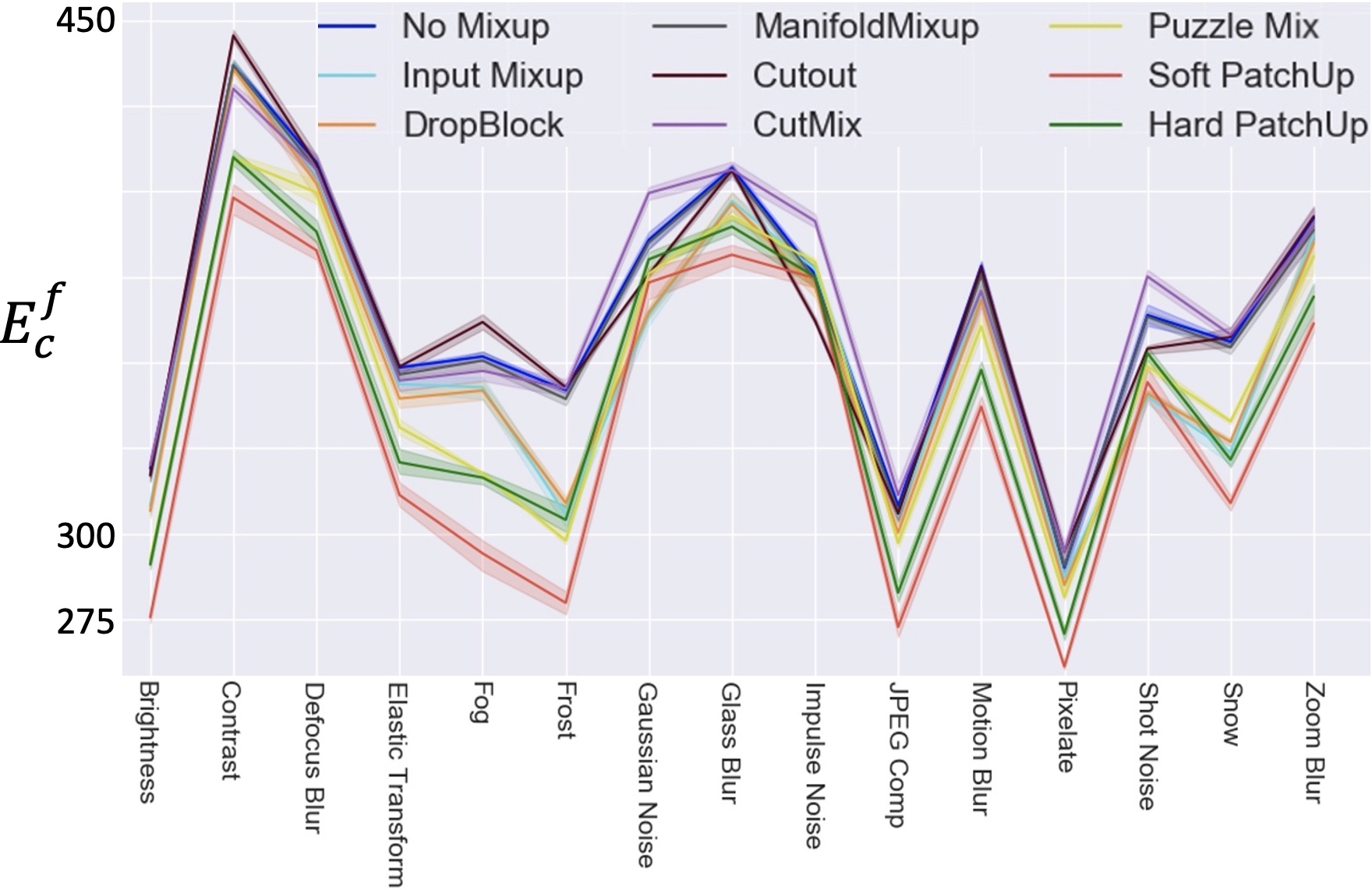
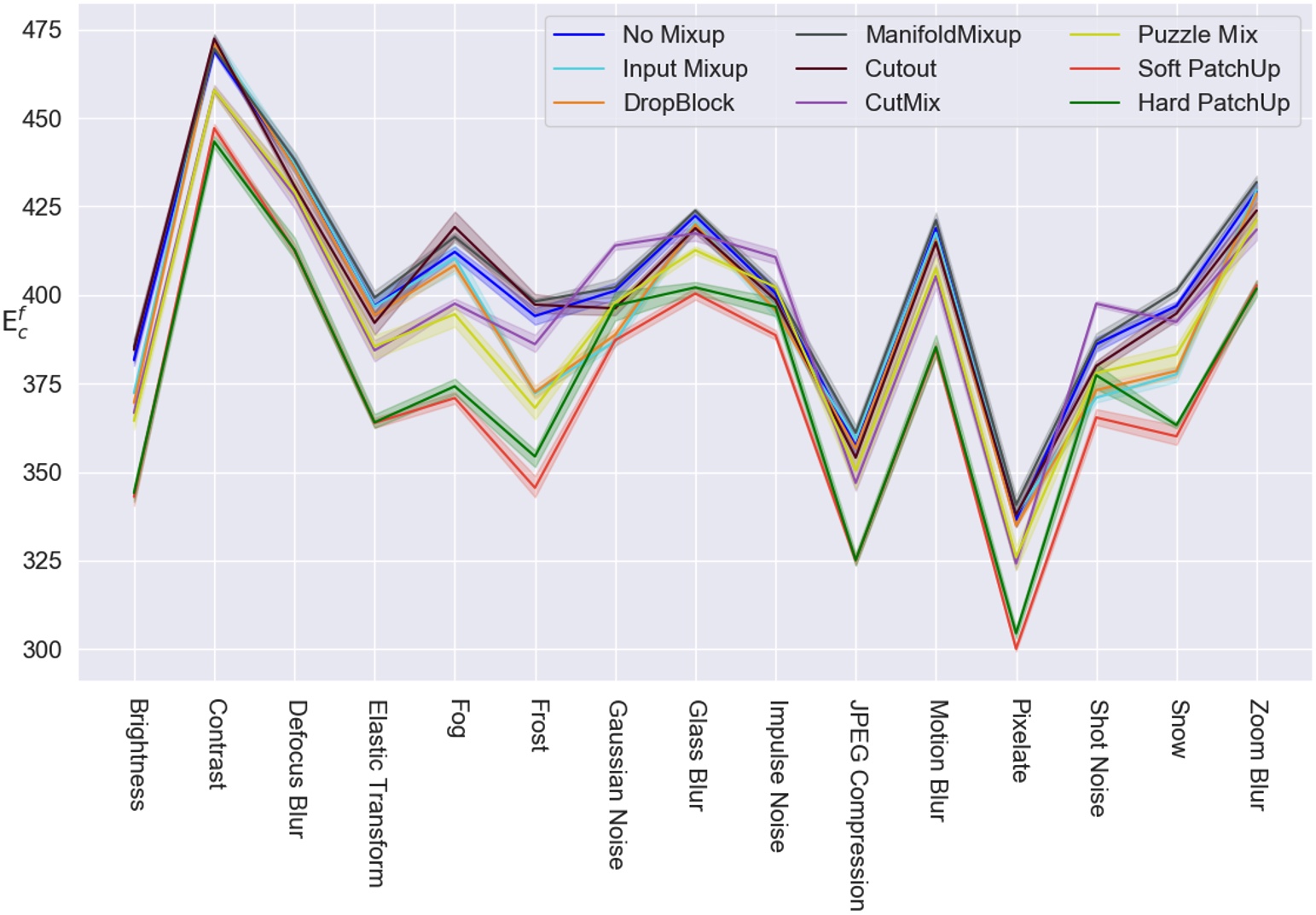
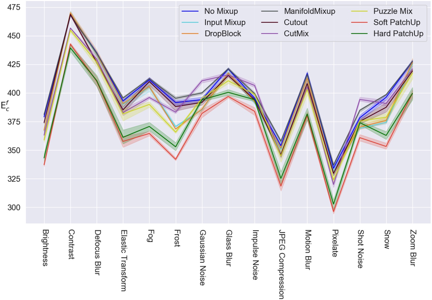
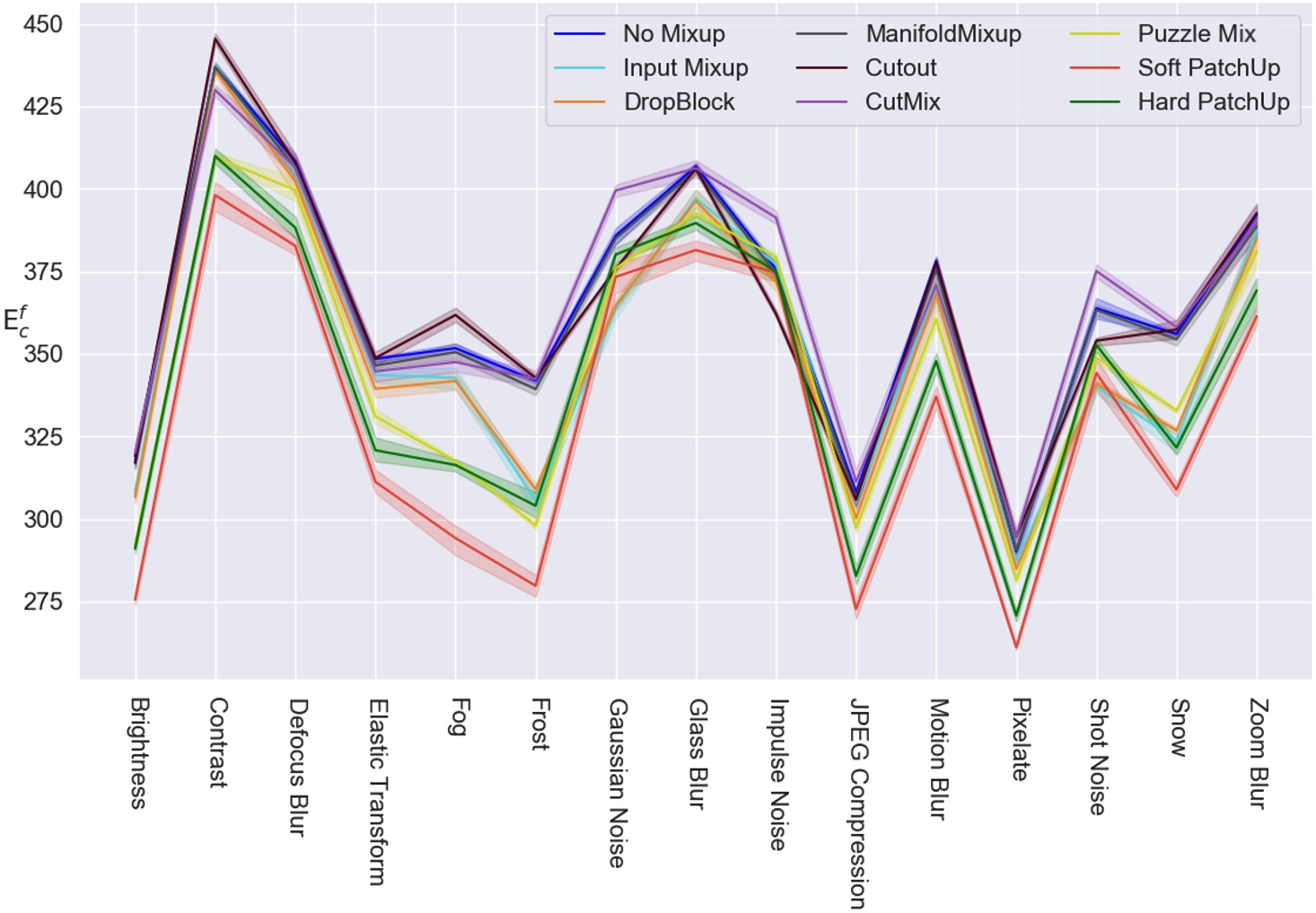
Robustness to Common Corruptions
The common corruption benchmark helps to evaluate the robustness of models against the input corruptions (Hendrycks and Dietterich 2019). It uses the 75 corruptions in 15 categories such that each has five levels of severity. We compare the methods robustness in Tiny-ImageNet-C for ResNet101/152, and WRN-28-10. So, we compute the sum of error denoted as where is the level of severity and is corruption type such that (Hendrycks and Dietterich 2019). Fig.4 shows Soft PatchUp leads the best performance in Tiny-ImageNet-C and Hard PatchUp achieves the second-best. Figures 15a and b in Appendix show the comparison results in ResNet101 and 152.
Generalization on Deformed Images
Affine transformations on the test set provide novel deformed data that can be used to evaluate the robustness of a method on out-of-distribution samples (Verma et al. 2019). We trained PreActResNet34 and WRN-28-10 on the CIFAR100. Then, we created a deformed test from CIFAR100 by applying some affine transformations. Table 4 shows that PatchUp provides the best performance on the affine transformed test and better generalization in PreActResNet34. Table 10 (F-appx.) shows that the quality of representations is improved by PatchUp and it shows better generalization in the deformed test on WRN-28-10. Generalization is significantly improved by PatchUp over existing methods by a large margin, as is the quality of representations.
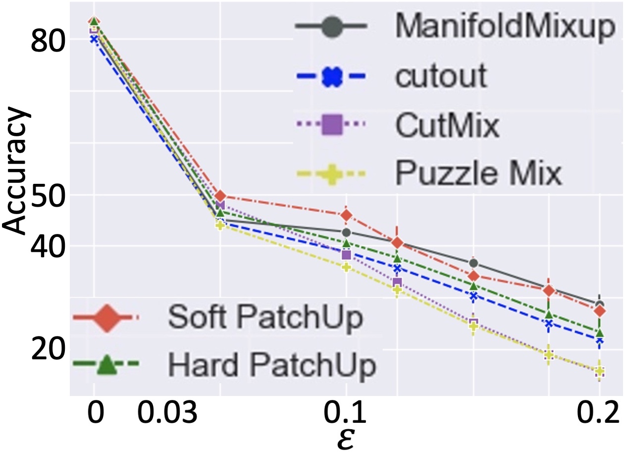
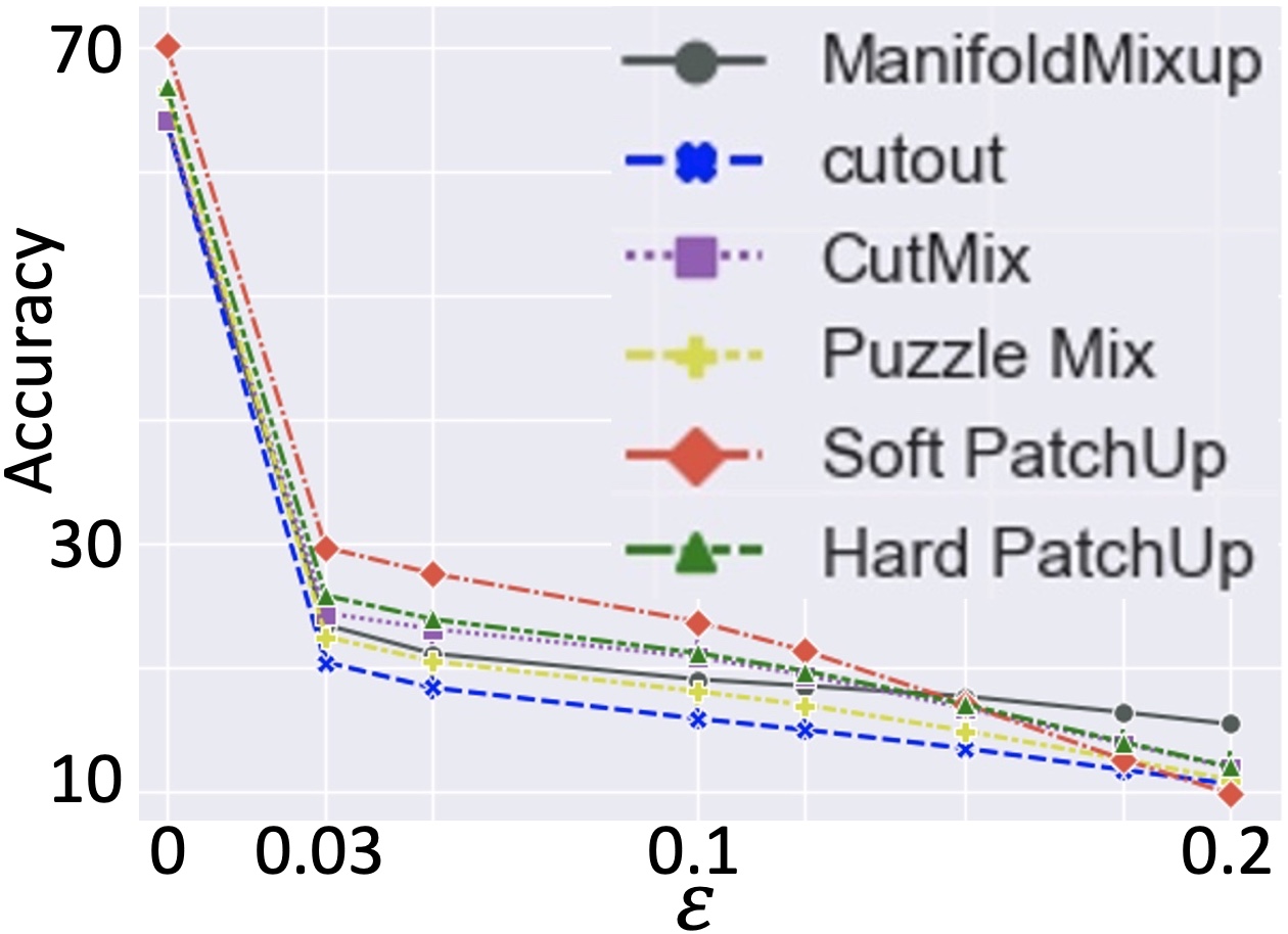
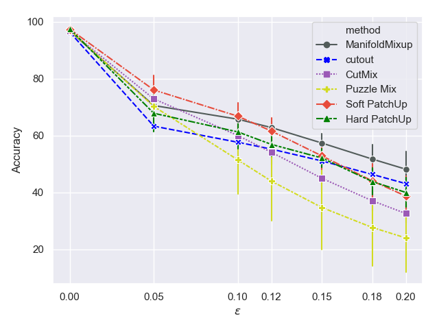
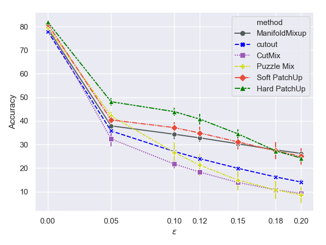
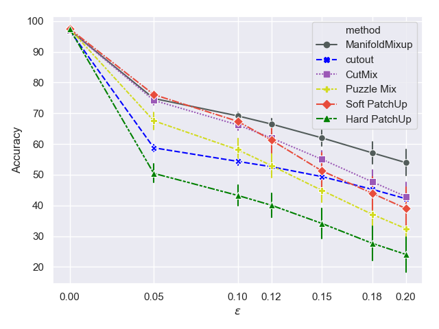
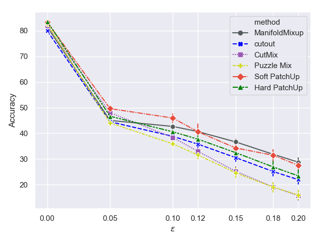
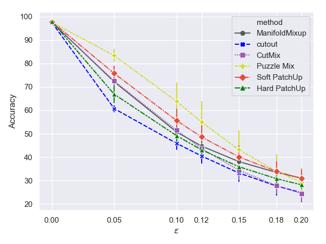
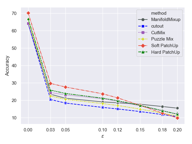
Robustness to Adversarial Examples
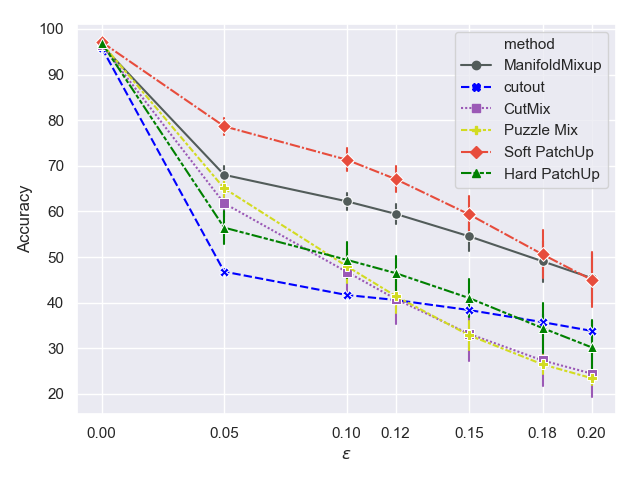
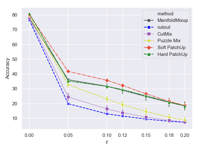
Neural networks, trained with ERM, are often vulnerable to adversarial examples (Szegedy et al. 2013). Certain data-dependent methods can alleviate such fragility to adversarial examples by training the models with interpolated data. So, the robustness of a regularized model to adversarial examples can be considered as a criterion for comparison (Zhang et al. 2017; Verma et al. 2019). Fig.5 compares the performance of the methods on CIFAR100 and Tiny-ImageNet with adversarial examples created by the FGSM attack described in (Goodfellow, Shlens, and Szegedy 2014). Fig 13-appx. contains further comparison on PreActResNet18/34 and WRN-28-10 for CIFAR10 and SVHN with FGSM attacks. Table 5 shows the robust accuracy (in the range of ) for the Foolbox benchmark (Rauber, Brendel, and Bethge 2018) against the 7-steps DeepFool (Moosavi-Dezfooli, Fawzi, and Frossard 2016), Decoupled Direction and Norm (DDN) (Rony et al. 2019), Carlini-Wagner (CW) (Carlini and Wagner 2017), and (Madry et al. 2019) attacks with . We observe that PatchUp is more robust to adversarial attacks compared to other methods. While Hard PatchUp achieves better performance in terms of classification accuracy, Soft PatchUp seems to trade off a slight loss of accuracy in order to achieve more robustness.
| Methods | DeepFool | DDN | CW | |
|---|---|---|---|---|
| No Mixup | ||||
| Input Mixup | ||||
| ManifoldMixup | ||||
| Cutout | ||||
| DropBlock | ||||
| CutMix | ||||
| Puzzle Mix | ||||
| Soft PatchUp | ||||
| Hard PatchUp |
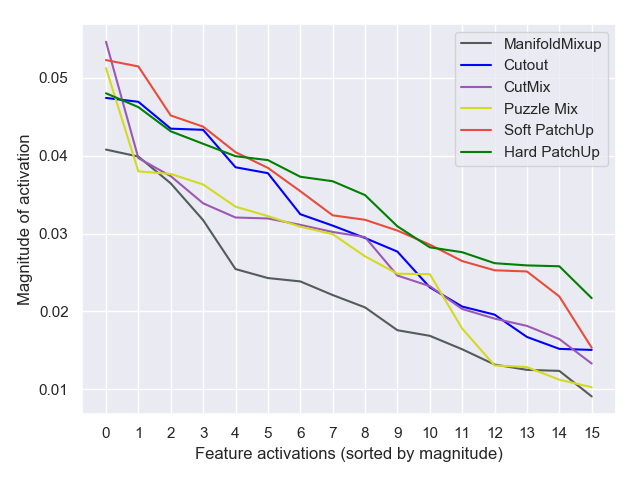
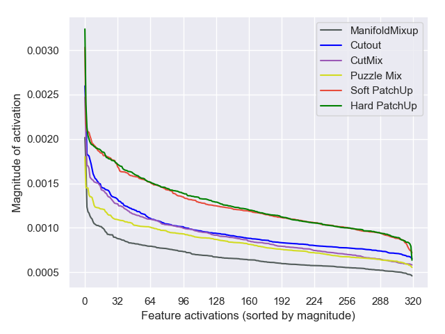
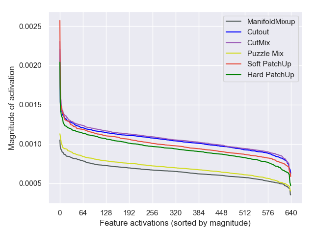
Effect on Activations
To study the effect of the methods on the activations in the residual blocks, we compared the mean magnitude of feature activations in the residual blocks following (DeVries and Taylor 2017) in WRN-28-10 for CIFAR100 test set. We train the models with each method and then calculate the magnitudes of activations in the test set. The higher mean magnitude of features shows that the models tried to produce a wider variety of features in the residual blocks (DeVries and Taylor 2017). Our WRN-28-10 has a conv2d module followed by three residual blocks. We selected randomly such that . And, we apply the ManifoldMixup and PatchUp in either input space, the first conv2d, and the first or second residual blocks (results in Fig.7).
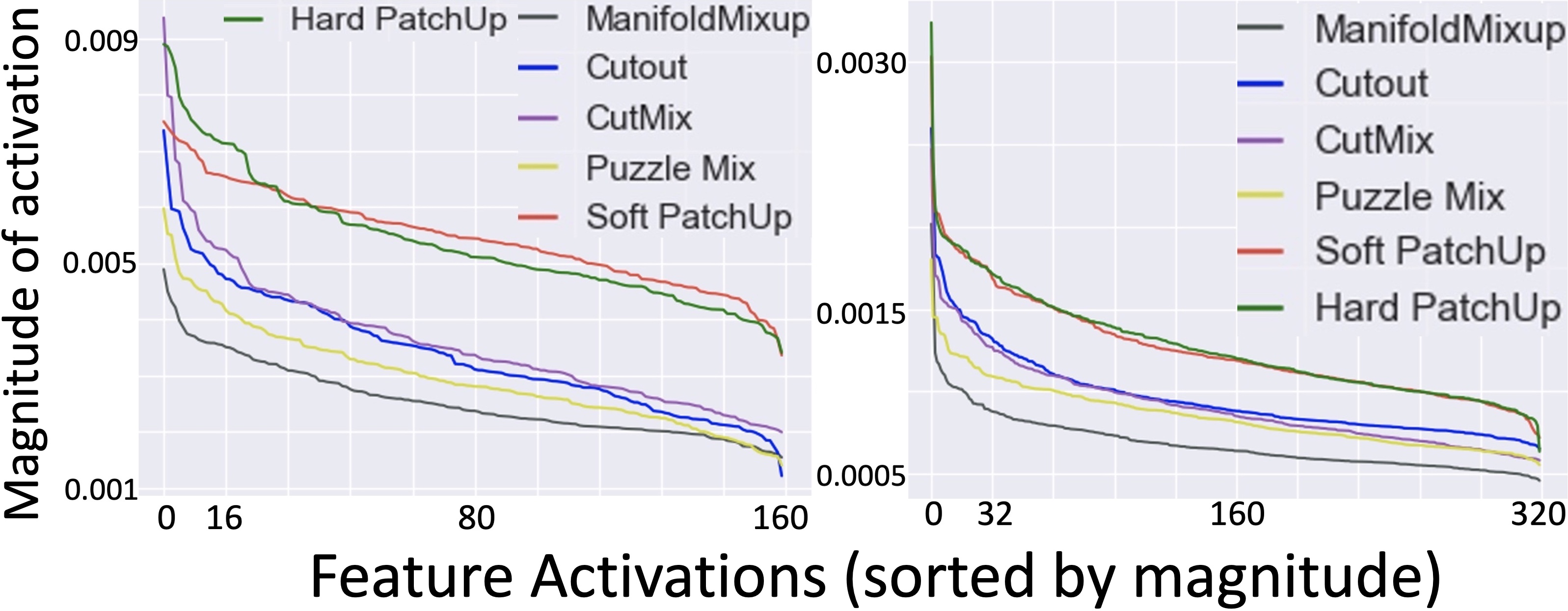
Figure 7 shows that PatchUp produces more diverse features in the layers where we apply PatchUp. Fig. 14-appx. shows the results in the first conv2d, first residual, second residual, and third residual blocks. Since we are not applying the PatchUp in the third residual block, the mean magnitude of the feature activations are below, but very close to, Cutout and CutMix. This also shows that producing a wide variety of features can be an advantage for a model. But, according to our experiments, a larger magnitude of activations does not always lead to better performance. Fig.7 shows that for ManifoldMixup, the mean magnitude of the feature activations is less than others. But, it performs better than Cutout and CutMix in most tasks.
Significance of loss terms and analysis of k
PatchUp uses the loss that is introduced in Equation 6. We can paraphrase the PatchUp learning objective for this ablation study as follows:
| (10) |
where and . We also show the effect of and in PatchUp loss. Table 6 shows the error rate on the validation set for WRN-28-10 on CIFAR100. This shows the summation of the and reduces error rate by in PatchUp. We conducted an experiment to show the importance of random layer selection in PatchUp. Table 7 shows the contribution of the random selection of the layer in the overall performance of the method. In the left-most column 1/2/3 refers to PatchUp being applied to only one layer (more details in section “B” in appx.).
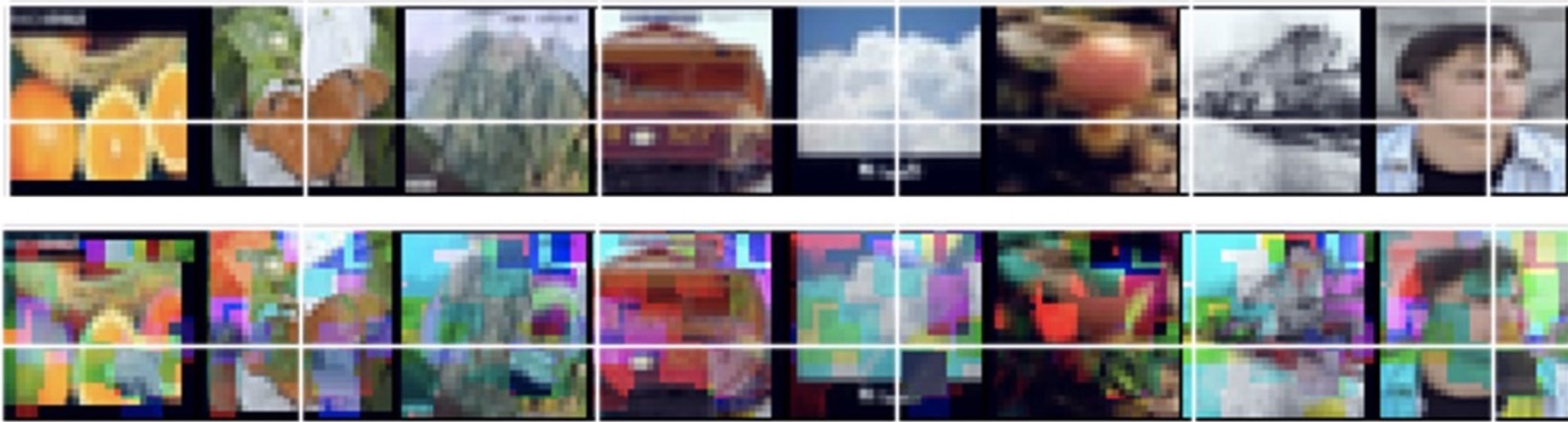
As noted in section “2”, the PatchUp mask is “too strong” for the input space. Fig.8 shows that the PatchUp mask often drastically destroys the semantic concepts in the input images. Thus, we select one random rectangular patch in the input space (similar to CutMix). However, the learning objective in (k = 0) is still the PatchUp objective that is different from CutMix. The last row in table 7 shows the negative effect of applying the PatchUp mask in the input space.
| Simple | Error Rate: | ||
|---|---|---|---|
| WRN-28-10 | |||
| Error with | Error with | Error with | |
| Soft PatchUp | |||
| Hard PatchUp | |||
| layer | Val Error | Test Error | Test NLL |
| Random selection | |||
| PatchUp Masks in | |||
5 Conclusion
We presented PatchUp, a simple and efficient regularizer scheme for CNNs that alleviates some of the drawbacks of the previous mixing-based regularizers. Our experimental results show that with the proposed approach, PatchUp, we can achieve state-of-the-art results on image classification tasks across different architectures and datasets. Similar to previous mixing-based approaches, our approach also has the advantage of avoiding any added computational overhead. The strong test accuracy achieved by PatchUp, with no additional computational overhead, makes it particularly appealing for practical applications.
6 Acknowledgments
We would like to acknowledge Compute Canada and Calcul Quebec for providing the computing resources used in this work. The authors would also like to thank Damien Scieur, Hannah Alsdurf, Alexia Jolicoeur-Martineau, and Yassine Yaakoubi for reviewing the manuscript. SC is supported by a Canada CIFAR AI Chair and an NSERC Discovery Grant.
References
- Achille and Soatto (2018) Achille, A.; and Soatto, S. 2018. Information Dropout: Learning Optimal Representations Through Noisy Computation. IEEE Transactions on Pattern Analysis and Machine Intelligence, 40(12): 2897–2905.
- Arpit et al. (2017) Arpit, D.; Jastrzebski, S.; Ballas, N.; Krueger, D.; Bengio, E.; Kanwal, M. S.; Maharaj, T.; Fischer, A.; Courville, A.; Bengio, Y.; et al. 2017. A closer look at memorization in deep networks. In Proceedings of the 34th International Conference on Machine Learning-Volume 70, 233–242. JMLR. org.
- Carlini and Wagner (2017) Carlini, N.; and Wagner, D. 2017. Towards evaluating the robustness of neural networks. In 2017 ieee symposium on security and privacy (sp), 39–57. IEEE.
- Chrabaszcz, Loshchilov, and Hutter (2017) Chrabaszcz, P.; Loshchilov, I.; and Hutter, F. 2017. A Downsampled Variant of ImageNet as an Alternative to the CIFAR datasets. arXiv:1707.08819.
- Cubuk et al. (2019) Cubuk, E. D.; Zoph, B.; Mane, D.; Vasudevan, V.; and Le, Q. V. 2019. AutoAugment: Learning Augmentation Policies from Data. arXiv:1805.09501.
- DeVries and Taylor (2017) DeVries, T.; and Taylor, G. W. 2017. Improved Regularization of Convolutional Neural Networks with Cutout. arXiv:1708.04552.
- Gal and Ghahramani (2016) Gal, Y.; and Ghahramani, Z. 2016. A theoretically grounded application of dropout in recurrent neural networks. In Advances in neural information processing systems, 1019–1027.
- Ghiasi, Lin, and Le (2018) Ghiasi, G.; Lin, T.; and Le, Q. V. 2018. DropBlock: A regularization method for convolutional networks. CoRR, abs/1810.12890.
- Goodfellow, Bengio, and Courville (2016) Goodfellow, I.; Bengio, Y.; and Courville, A. 2016. Deep learning. MIT press.
- Goodfellow, Shlens, and Szegedy (2014) Goodfellow, I. J.; Shlens, J.; and Szegedy, C. 2014. Explaining and Harnessing Adversarial Examples. arXiv:1412.6572.
- Guo, Mao, and Zhang (2018) Guo, H.; Mao, Y.; and Zhang, R. 2018. MixUp as Locally Linear Out-Of-Manifold Regularization. CoRR, abs/1809.02499.
- He et al. (2015) He, K.; Zhang, X.; Ren, S.; and Sun, J. 2015. Deep Residual Learning for Image Recognition. CoRR, abs/1512.03385.
- He et al. (2016) He, K.; Zhang, X.; Ren, S.; and Sun, J. 2016. Identity Mappings in Deep Residual Networks. arXiv:1603.05027.
- Hendrycks and Dietterich (2019) Hendrycks, D.; and Dietterich, T. 2019. Benchmarking Neural Network Robustness to Common Corruptions and Perturbations. arXiv:1903.12261.
- Hendrycks et al. (2020) Hendrycks, D.; Mu, N.; Cubuk, E. D.; Zoph, B.; Gilmer, J.; and Lakshminarayanan, B. 2020. AugMix: A Simple Data Processing Method to Improve Robustness and Uncertainty. arXiv:1912.02781.
- Hinton et al. (2012) Hinton, G.; Deng, L.; Yu, D.; Dahl, G. E.; Mohamed, A.; Jaitly, N.; Senior, A.; Vanhoucke, V.; Nguyen, P.; Sainath, T. N.; and Kingsbury, B. 2012. Deep Neural Networks for Acoustic Modeling in Speech Recognition: The Shared Views of Four Research Groups. IEEE Signal Processing Magazine, 29(6): 82–97.
- Kim, Choo, and Song (2020) Kim, J.-H.; Choo, W.; and Song, H. O. 2020. Puzzle Mix: Exploiting Saliency and Local Statistics for Optimal Mixup. arXiv:2009.06962.
- Kingma, Salimans, and Welling (2015) Kingma, D. P.; Salimans, T.; and Welling, M. 2015. Variational dropout and the local reparameterization trick. Advances in neural information processing systems, 28: 2575–2583.
- Kingma and Welling (2013) Kingma, D. P.; and Welling, M. 2013. Auto-encoding variational bayes. arXiv preprint arXiv:1312.6114.
- Krizhevsky (2009) Krizhevsky, A. 2009. Learning Multiple Layers of Features from Tiny Images.
- Krizhevsky, Sutskever, and Hinton (2012) Krizhevsky, A.; Sutskever, I.; and Hinton, G. E. 2012. ImageNet Classification with Deep Convolutional Neural Networks. In Pereira, F.; Burges, C. J. C.; Bottou, L.; and Weinberger, K. Q., eds., Advances in Neural Information Processing Systems 25, 1097–1105. Curran Associates, Inc.
- Krueger et al. (2016) Krueger, D.; Maharaj, T.; Kramár, J.; Pezeshki, M.; Ballas, N.; Ke, N. R.; Goyal, A.; Bengio, Y.; Courville, A.; and Pal, C. 2016. Zoneout: Regularizing rnns by randomly preserving hidden activations. arXiv preprint arXiv:1606.01305.
- Madry et al. (2019) Madry, A.; Makelov, A.; Schmidt, L.; Tsipras, D.; and Vladu, A. 2019. Towards Deep Learning Models Resistant to Adversarial Attacks. arXiv:1706.06083.
- Mai et al. (2019) Mai, Z.; Hu, G.; Chen, D.; Shen, F.; and Shen, H. T. 2019. MetaMixUp: Learning Adaptive Interpolation Policy of MixUp with Meta-Learning. arXiv:1908.10059.
- Moosavi-Dezfooli, Fawzi, and Frossard (2016) Moosavi-Dezfooli, S.-M.; Fawzi, A.; and Frossard, P. 2016. Deepfool: a simple and accurate method to fool deep neural networks. In Proceedings of the IEEE conference on computer vision and pattern recognition, 2574–2582.
- Netzer et al. (2011) Netzer, Y.; Wang, T.; Coates, A.; Bissacco, A.; Wu, B.; and Ng, A. Y. 2011. Reading Digits in Natural Images with Unsupervised Feature Learning. In NIPS Workshop on Deep Learning and Unsupervised Feature Learning 2011.
- Rauber, Brendel, and Bethge (2018) Rauber, J.; Brendel, W.; and Bethge, M. 2018. Foolbox: A Python toolbox to benchmark the robustness of machine learning models. arXiv:1707.04131.
- Ren et al. (2015) Ren, S.; He, K.; Girshick, R.; and Sun, J. 2015. Faster R-CNN: Towards Real-Time Object Detection with Region Proposal Networks. In Cortes, C.; Lawrence, N. D.; Lee, D. D.; Sugiyama, M.; and Garnett, R., eds., Advances in Neural Information Processing Systems 28, 91–99. Curran Associates, Inc.
- Rony et al. (2019) Rony, J.; Hafemann, L. G.; Oliveira, L. S.; Ayed, I. B.; Sabourin, R.; and Granger, E. 2019. Decoupling Direction and Norm for Efficient Gradient-Based L2 Adversarial Attacks and Defenses. In Proceedings of the IEEE/CVF Conference on Computer Vision and Pattern Recognition (CVPR).
- Russakovsky et al. (2015) Russakovsky, O.; Deng, J.; Su, H.; Krause, J.; Satheesh, S.; Ma, S.; Huang, Z.; Karpathy, A.; Khosla, A.; Bernstein, M.; Berg, A. C.; and Fei-Fei, L. 2015. ImageNet Large Scale Visual Recognition Challenge. arXiv:1409.0575.
- Srivastava et al. (2014) Srivastava, N.; Hinton, G.; Krizhevsky, A.; Sutskever, I.; and Salakhutdinov, R. 2014. Dropout: A Simple Way to Prevent Neural Networks from Overfitting. Journal of Machine Learning Research, 15: 1929–1958.
- Sutskever, Vinyals, and Le (2014) Sutskever, I.; Vinyals, O.; and Le, Q. V. 2014. Sequence to Sequence Learning with Neural Networks. In Proceedings of the 27th International Conference on Neural Information Processing Systems - Volume 2, NIPS’14, 3104–3112. Cambridge, MA, USA: MIT Press.
- Szegedy et al. (2013) Szegedy, C.; Zaremba, W.; Sutskever, I.; Bruna, J.; Erhan, D.; Goodfellow, I.; and Fergus, R. 2013. Intriguing properties of neural networks. arXiv preprint arXiv:1312.6199.
- Tishby and Zaslavsky (2015) Tishby, N.; and Zaslavsky, N. 2015. Deep Learning and the Information Bottleneck Principle. CoRR, abs/1503.02406.
- Tompson et al. (2014a) Tompson, J.; Goroshin, R.; Jain, A.; LeCun, Y.; and Bregler, C. 2014a. Efficient Object Localization Using Convolutional Networks. CoRR, abs/1411.4280.
- Tompson et al. (2014b) Tompson, J.; Goroshin, R.; Jain, A.; LeCun, Y.; and Bregler, C. 2014b. Efficient Object Localization Using Convolutional Networks. CoRR, abs/1411.4280.
- Vaswani et al. (2017) Vaswani, A.; Shazeer, N.; Parmar, N.; Uszkoreit, J.; Jones, L.; Gomez, A. N.; Kaiser, L.; and Polosukhin, I. 2017. Attention Is All You Need. CoRR, abs/1706.03762.
- Verma et al. (2019) Verma, V.; Lamb, A.; Beckham, C.; Najafi, A.; Mitliagkas, I.; Lopez-Paz, D.; and Bengio, Y. 2019. Manifold Mixup: Better Representations by Interpolating Hidden States. In Chaudhuri, K.; and Salakhutdinov, R., eds., Proceedings of the 36th International Conference on Machine Learning, volume 97 of Proceedings of Machine Learning Research, 6438–6447. Long Beach, California, USA: PMLR.
- Yun et al. (2019) Yun, S.; Han, D.; Oh, S. J.; Chun, S.; Choe, J.; and Yoo, Y. 2019. CutMix: Regularization Strategy to Train Strong Classifiers with Localizable Features. arXiv:1905.04899.
- Zagoruyko and Komodakis (2017) Zagoruyko, S.; and Komodakis, N. 2017. Wide Residual Networks. arXiv:1605.07146.
- Zhang et al. (2017) Zhang, H.; Cisse, M.; Dauphin, Y. N.; and Lopez-Paz, D. 2017. mixup: Beyond Empirical Risk Minimization. arXiv:1710.09412.
Appendices
Appendix A Algorithm
In this appendix, we provide a detailed algorithm for implementing PatchUp. As with most regularization techniques, PatchUp also has two modes (either inference or training). It also needs the combining type (either Soft PatchUp or Hard PatchUp), , and . This algorithm shows how PatchUp generates a new hidden representation from and . Lines 4 to 9 in the algorithm1 are the binary mask creation process used in both Soft PatchUp and Hard PatchUp.
Input:
: the hidden representation for the sample at layer .
: the hidden representation for the sample at layer .
either inference or training.
: soft or hard.
: the probability of altering a feature.
: the size of each block in the binary mask.
Output
, : original labels for samples and .
: the new hidden representation computed by PatchUp.
: The portion of the feature maps that remained unchanged.
: the target corresponding to the changed features.
: re-weighted target according to the interpolation policy.
Figure 11 briefly illustrates and summarizes the binary mask creation process in PatchUp. Lines 11 to 25 correspond to the interpolation and combination of hidden representations in the mini-batch in PatchUp. Figure 9 compares the masks generated by PatchUp and CutMix.
Appendix B Why random ?
PatchUp applies block-level regularization at a randomly selected hidden representation layer . The Information Bottleneck (IB) principle, introduced by Tishby and Zaslavsky (2015), gives a formal intuition for selecting randomly. First, let us encapsulate the layers of the network into blocks where each block could contain more than one layer. Let be the -th block of layers. In this case, sequential blocks share the information as a hidden representation to the next block of layers, sequentially. We can consider this case as a Markov chain of the block of layers as follows:
| (11) |
In this scenario, the sequential communication between the intermediate hidden representations are considered to be an information bottleneck. Therefore,
| (12) |
where is the mutual information between the -th and -th layer.
If has enough information to represent , then applying regularization techniques in will provide a better generalization to unseen data. However, most of the current state-of-the-art CNN models contain residual connections which break the Markov chain described above (since information can skip the layer). One solution to this challenge is to randomly select a residual block and apply regularization techniques like ManifoldMixup or PatchUp.

Appendix C PatchUp Interpolation Policy Effect
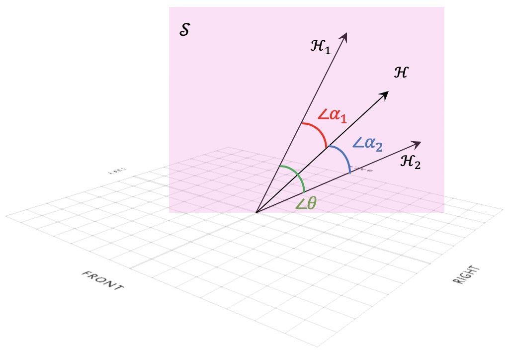
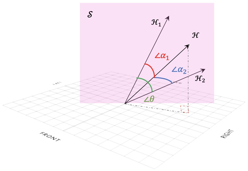
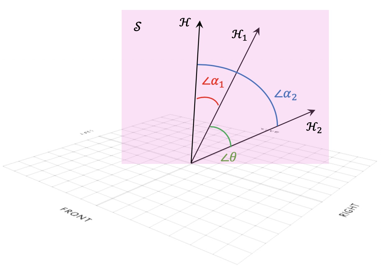
Assume that and are flattened hidden representations of two examples produced at layer . And, is the flattened interpolated hidden representation of these two paired samples at layer . First, we calculate the cosine distance of the pairs (, ), (, ), and (, ). Reversing the cosine of these cosine similarities give the angular distance between each pair of vectors denoted as , , and , respectively. There is always a surface that contains and denoted as . Mathematically, we have:
| (13) |
Let us define and . According to the triangle inequality principle, either or will be zero if, and only if, . Figure 12 illustrates three possible scenarios for two paired flattened hidden representations and their flattened interpolated hidden representations. and are zero for the left and right figures, respectively. We try to empirically show that , , and always lie in the same surface and lies between and in ManifoldMixup. This means that for ManifoldMixup because of its linear interpolation policy. The middle figure in 12 is the case that both and are not equal to zero. This figure shows that one possible situation is that flattened interpolated hidden representation does not lie in the surface . Our goal is to produce the interpolated hidden representation that lies in all possible places towards all dimensions in the hidden space.
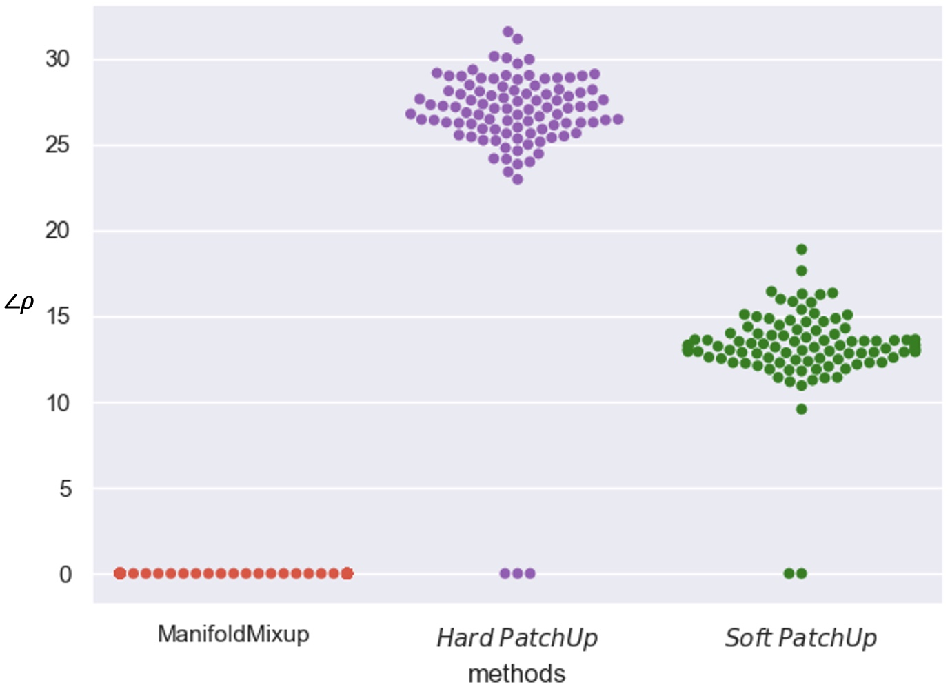
As discussed in section 3, ManifoldMixup can provide interpolated hidden representation only in a limited space. However, Soft PatchUp and Hard PatchUp can produce a wide variety of interpolated hidden representations towards different dimensions. To support that, in WideResNet-28-10, for a mini-batch of 100 samples, we calculated the for the flattened interpolated hidden representation produced by ManifoldMixup, Hard PatchUp, and Soft PatchUp at the second residual block (layer ) with the same interpolation policy (, , and ) for both Soft PatchUp and Hard PatchUp for all samples in the mini-batch. The swarmplot 11 shows all for the mini-batch are equal to zero in ManifoldMixup, which empirically supports our hypothesis. However, PatchUp produces more diverse interpolated hidden representations towards all dimensions in the hidden space. It is worth mentioning that few that are equal to zero in Soft PatchUp and Hard PatchUp belong to the interpolated hidden representation that was constructed from the pairs with the same labels.
Appendix D PatchUp Experiment Setup and Hyper-parameter Tuning
We follow the ManifoldMixup in our experiment setup, we use SGD with 0.9 Nesterov momentum as an optimizer, mini-batch of 100, and weight decay of 1e-4 (Verma et al. 2019).
This section describes the hyper-parameters of each model in table 9 following the hyper-parameter setup from ManifoldMixup (Verma et al. 2019) experiments in order to create a fair comparison. First, we performed hyper-parameter tuning for the PatchUp to achieve the best validation performance. Then we ran all the experiments five times, reporting the mean and standard deviation of errors and negative log-likelihoods for the selected models. We let models train for defined epochs and checkpoint the best model in terms of validation performance during the training. In our study, we used PreActResNet18, PreActResNet34, and WideResNet-28-10 models. Table 9 shows the hyper-parameters used for training the models.
| CIFAR (hours) | SVHN (hours) | Tiny-ImageNet (hours) | ||||||
|---|---|---|---|---|---|---|---|---|
| PatchUp | Puzzle Mix | PatchUp | Puzzle Mix | PatchUp | Puzzle Mix | |||
| PreActResNet18 | - | - | ||||||
| PreActResNet34 | - | - | ||||||
| WideResNet-28-10 | ||||||||

| Model | lr | lr steps | step factor | Epochs |
|---|---|---|---|---|
| PreactResnet18 | -- | |||
| PreactResnet34 | -- | |||
| WideResnet-28-10 | - |
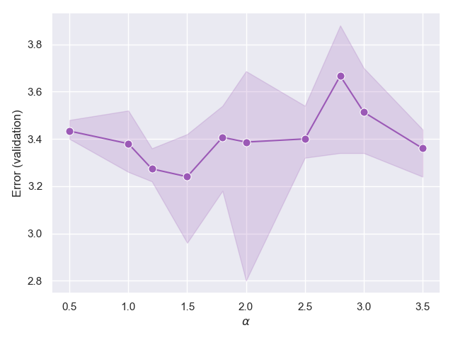
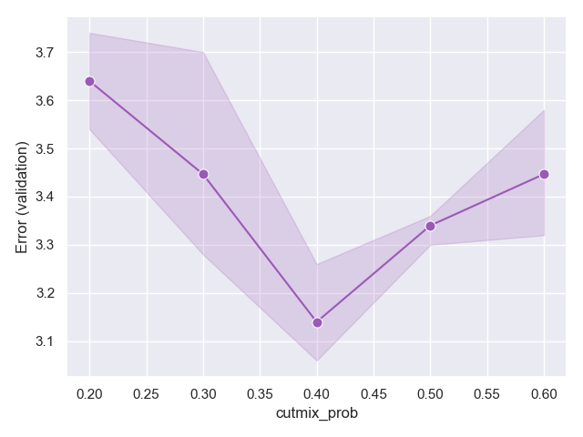
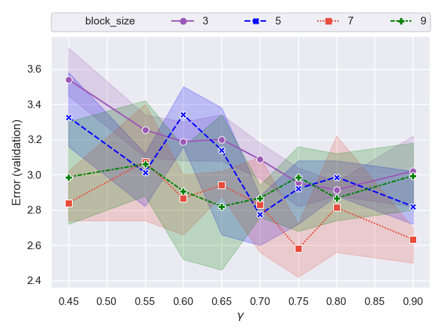
PatchUp adds , and as hyper-parameters. is the probability that the PatchUp operation is performed for a given mini-batch, i.e if there are mini-batches and is , PatchUp is performed in fraction of mini-batches. and are described in section 2. We tuned the PatchUp hyper-parameter on CIFAR10 with the PreActResNet18. To create a validation set, we split of training samples into a validation set. We set to in PatchUp. For Soft PatchUp, we set to and applied PatchUp to all mini-batches in training. Then, we did a grid search by varying from to and from to . We found that of and of work best for Soft PatchUp as shown in figure 13(c). Similarly, for Hard PatchUp, we set to and performed a grid search by varying from to and from to . We found that of and of yield the best results for Hard PatchUp as shown in figure 13(d). Figure 13(a) shows that ManifoldMixup with () achieves the best validation performance. For cutout, we used the same hyper-parameters proposed in (DeVries and Taylor 2017), setting cutout to for CIFAR10, for CIFAR100, and for SVHN following (DeVries and Taylor 2017). Figure 13(b) shows that CutMix achieves its best validation performance in PreActResNet18 in CIFAR10 with . Furthermore, DropBlock achieves its best validation performance on this task by setting the block size and to and , respectively (Ghiasi, Lin, and Le 2018). To train models using regularization methods, we use one GPU (v100). The training time for other methods is almost the same as PatchUp since they are not adding any computational overhead. But, Puzzle Mix adds about three times and two times more computational overhead in SVHN, CIFAR, and Tiny-ImageNet, respectively. Table 8 show the training time comparison.
As we showed in our ablation study (shown in Figure 8 and Table 7). Applying the PatchUp Mask in input space drastically destroys the semantic concepts in the input images (Figure8). Also worth mentioning is that it is unlikely that applying the PatchUp Mask in latent space leads to drastically changing the hidden representation since we have many channels. Tuning gamma as a hyperparameter will prevent such large semantic changes in the latent space. However, gamma cannot avoid such negative effects in input space. As per Table 7, applying the CutMix Binary Mask in input space but still using the PatchUp learning objective leads to a performance improvement of when training WRN-28-10 on CIFAR-100, which is significant when considering the tight competition between regularization methods.
Appendix E Further explanation on PatchUp and its learning objective:
According to the Eq. 4 is computed as follows:
In the first term in equation 6, we take a convex combination of the following two loss functions: one with respect to the unchanged part of the feature maps () and the other with respect to the interpolated part (). Please note that the loss function for the interpolated part will change based on whether we do Soft or Hard PatchUp. Therefore, we can expand the PatchUp learning objective as follows:
Based on the operation defined in section 2, we can substitute and expand the learning objective for Hard PatchUp as follows: (For Soft PatchUp the process will be similar.) In the Hard PatchUp:
And according to Equation 8,
Therefore, we can conclude the learning objective for Hard PatchUp is defined as follows:
where the . Hard PatchUp is a fully differentiable operation. The masks for the hard PatchUp are sampled outside the computation graph and passed as input to the architecture. Hence the entire architecture is differentiable end-to-end. This is similar to the reparameterization trick that was proposed in (Kingma and Welling 2013). A similar trick was also applied in Variational Dropout (Kingma, Salimans, and Welling 2015) and other similar methods as well. Similarly, we can substitute the operations ( and defined in Equation 3 and 5) to expand the learning objective of Soft PatchUp.
PatchUp works by applying a structured noisy process to the representations at a random point in the forward pass (random layer). The model then learns to recognize the structure in the noisy representations created in the forward pass by back-propagating through the model with the gradients from the PatchUp learning objective. Since all operations are differentiable and involve either swapping or mixing latent spaces (similar to the reparameterization trick), we will not have any non-differentiability issues when calculating the gradients. Hence, deriving the backprop manually is not necessary.
Appendix F Generalization on Deformed Images
| Transformation | cutout | CutMix | ManifoldMixup | Puzzle Mix | Soft PatchUp | Hard PatchUp |
|---|---|---|---|---|---|---|
| Rotate (-20, 20) | ||||||
| Rotate (-40, 40) | ||||||
| Shear (-28.6, 28.6) | ||||||
| Shear (-57.3, 57.3) | ||||||
| Scale (0.6) | ||||||
| Scale (0.8) | ||||||
| Scale (1.2) | ||||||
| Scale (1.4) |
We created the deformed test sets from CIFAR100, as described in Section 4. Table 10 shows improved quality of representations learned by a WideResNet-28-10 model regularized by PatchUp on CIFAR100 deformed test sets. The significant improvements in generalization provided by PatchUp in this experiment shows the high quality of representations learned with PatchUp.
Appendix G Robustness to Adversarial Examples
The adversarial attacks refer to small and unrecognizable perturbations on the input images that can mislead deep learning models (Goodfellow, Shlens, and Szegedy 2014; Goodfellow, Bengio, and Courville 2016). One approach to creating adversarial examples is using the Fast Gradient Sign Method (FGSM), also known as a white-box attack (Goodfellow, Shlens, and Szegedy 2014). FGSM creates examples by adding small perturbations to the original examples. Once a regularized model is trained then FSGM creates adversarial examples as follows (Goodfellow, Shlens, and Szegedy 2014):
| (14) |
where is an adversarial example, is the original example, is the ground truth label for , and is the loss of the model with parameters of . controls the perturbation.
Our experiments show the effectiveness of Soft PatchUp against the attacks in most cases. However, Hard PatchUp performed well against the FGSM attack only on PreActResNet34 for CIFAR100. Figure 14 shows the comparison of the state-of-the-art regularization techniques’ effect on model robustness against the FGSM attack.
Appendix H Analysis of PatchUp’s Effect on Activations
In our implementation WideResNet28-10 has a conv2d module followed by three residual blocks. Figure 15 illustrates the comparison of ManifoldMixup, cutout, CutMix, Soft PatchUp, and Hard PatchUp. Figure 15(a), 15(b), and 15(c) show that PatchUp produces more variety of features in layers that we apply PatchUp on.

Appendix I More Details on Image Classification results
This section contains the image classification error and Test NLL on CIFAR10, CIFAR100, and SVHN datasets. Tables 12 and 11 shows Test error rates and test NLL on CIFAR10, CIFAR100, and SVHN datasets using PreActResNet18, PreActResNet34, and WideResNet-28-10 models.
When we have a data-scarce scenario, high-capacity models tend to memorize the examples. This leads to models with reasonable testing performance but that are very sensitive to small changes in test distribution as shown in Tiny-ImageNet-C experiments. Tiny-ImageNet has 200 classes while CIFAR-100 has 100 classes, and both datasets have 500 training examples per class. Our experiment shows that on the CIFAR-100 (the smaller dataset), all the data-dependent regularization methods tend to perform well. When we switch to Tiny-ImageNet (the larger dataset), the (non-PatchUp) data-dependent regularization methods are still effective, but not necessarily close to the best method (PatchUp) as shown in Table 12 and 1.
| PreActResNet18 | PreActResNet34 | WideResnet-28-10 | ||||||
|---|---|---|---|---|---|---|---|---|
| Error | Loss | Error | Loss | Eror | Loss | |||
| No Mixup | ||||||||
| Input Mixup ( = 1) | ||||||||
| ManifoldMixup (= 2) | ||||||||
| Cutout | ||||||||
| DropBlock | ||||||||
| CutMix | ||||||||
| Puzzle Mix | ||||||||
| Soft PatchUp | ||||||||
| Hard PatchUp | ||||||||
| PreActResNet18 | Test Error (%) | Test NLL | PreActResNet18 | Test Error (%) | Test NLL | |
| No Mixup | No Mixup | |||||
| Input Mixup ( = 1) | Input Mixup ( = 1) | |||||
| ManifoldMixup ( = 1.5) | ManifoldMixup ( = 1.5) | |||||
| Cutout | Cutout | |||||
| DropBlock | DropBlock | |||||
| CutMix | CutMix | |||||
| Puzzle Mix | Puzzle Mix | |||||
| Soft PatchUp | Soft PatchUp | |||||
| Hard PatchUp | Hard PatchUp | |||||
| PreActResNet34 | PreActResNet34 | |||||
| No Mixup | No Mixup | |||||
| Input Mixup ( = 1) | Input Mixup ( = 1) | |||||
| ManifoldMixup ( = 1.5) | ManifoldMixup ( = 1.5) | |||||
| Cutout | Cutout | |||||
| DropBlock | DropBlock | |||||
| CutMix | CutMix | |||||
| Puzzle Mix | Puzzle Mix | |||||
| Soft PatchUp | Soft PatchUp | |||||
| Hard PatchUp | Hard PatchUp | |||||
| WideResNet-28-10 | WideResNet-28-10 | |||||
| No Mixup | No Mixup | |||||
| Input Mixup ( = 1) | Input Mixup ( = 1) | |||||
| ManifoldMixup ( = 1.5) | ManifoldMixup ( = 1.5) | |||||
| Cutout | Cutout | |||||
| DropBlock | DropBlock | |||||
| CutMix | CutMix | |||||
| Puzzle Mix | Puzzle Mix | |||||
| Soft PatchUp | Soft PatchUp | |||||
| Hard PatchUp | Hard PatchUp | |||||
| Comparison on CIFAR-10 | Comparison on CIFAR-100 | |||||