Enabling Counterfactual Survival Analysis
with Balanced Representations

Abstract.

A clear and well-documented LaTeX document is presented as an article formatted for publication by ACM in a conference proceedings or journal publication. Based on the “acmart” document class, this article presents and explains many of the common variations, as well as many of the formatting elements an author may use in the preparation of the documentation of their work.

Abstract.

Balanced representation learning methods have been applied successfully to counterfactual inference from observational data. However, approaches that account for survival outcomes are relatively limited. Survival data are frequently encountered across diverse medical applications, i.e., drug development, risk profiling, and clinical trials, and such data are also relevant in fields like manufacturing (e.g., for equipment monitoring). When the outcome of interest is a time-to-event, special precautions for handling censored events need to be taken, as ignoring censored outcomes may lead to biased estimates. We propose a theoretically grounded unified framework for counterfactual inference applicable to survival outcomes. Further, we formulate a nonparametric hazard ratio metric for evaluating average and individualized treatment effects. Experimental results on real-world and semi-synthetic datasets, the latter of which we introduce, demonstrate that the proposed approach significantly outperforms competitive alternatives in both survival-outcome prediction and treatment-effect estimation.

1. INTRODUCTION

Survival analysis or time-to-event studies focus on modeling the time of a future event, such as death or failure, and investigate its relationship with covariates or predictors of interest. Specifically, we may be interested in the causal effect of a given intervention or treatment on survival time. A typical question may be: will a given therapy increase the chances of survival of an individual or population? Such causal inquiries on survival outcomes are common in the fields of epidemiology and medicine (Robins, 1986; Hammer et al., 1996; Yusuf et al., 2016). As an important current example, the COVID-19 pandemic is creating a demand for methodological development to address such questions, specifically, when evaluating the effectiveness of a potential vaccine or therapeutic outside randomized controlled trial settings.

Traditional causal survival analysis is typically carried out in the context of a randomized controlled trial (RCT), where the treatment assignment is controlled by researchers. Though they are the gold standard for causal inference, RCTs are usually long-term engagements, expensive and limited in sample size. Alternatively, the availability of observational data with comprehensive information about patients, such as electronic health records (EHRs), constitutes a more accessible but also more challenging source for estimating causal effects (Häyrinen et al., 2008; Jha et al., 2009). Such observational data may be used to augment and verify an RCT, after a particular treatment is approved and in use (Gombar et al., 2019; Frankovich et al., 2011; Longhurst et al., 2014). Moreover, the wealth of information from observational data also allows for the estimation of the individualized treatment effect (ITE), namely, the causal effect of an intervention at the individual level. In this work, we develop a novel framework for counterfactual time-to-event prediction to estimate the ITE for survival or time-to-event outcomes from observational data.

Estimating the causal effect for survival outcomes in observational data manifests two principal challenges. First, the treatment assignment mechanism is not known a priori. Therefore, there may be variables, known as confounders, affecting both the treatment and survival time, which lead to selection bias (Bareinboim and Pearl, 2012), i.e., that the distributions across treatment groups are not the same. In this work, we focus on selection biases due to confounding, but other sources may also be considered. For instance, patients who are severely ill are likely to receive more aggressive therapy, however, their health status may also inevitably influence survival. Traditional survival analysis neglects such bias, leading to incorrect causal estimation. Second, the exact time-to-event is not always observed, i.e., sometimes we only know that an event has not occurred up to a certain point in time. This is known as the censoring problem. Moreover, censoring might be informative depending on the characteristics of the individuals and their treatment assignments, thus proper adjustment is required for accurate causal estimation (Cole and Hernán, 2004; Díaz, 2019).

Traditional causal survival-analysis approaches typically model the effect of the treatment or covariates (not time or survival) in a parametric manner. Two commonly used models are the Cox proportional hazards (CoxPH) model (Cox, 1972) and the accelerated failure time (AFT) model (Wei, 1992), which presume a linear relationship between the covariates and survival probability. Further, proper weighting for each individual has been employed to account for confounding bias from these models (Austin, 2007, 2014; Hernán et al., 2005). For instance, probability weighting schemes that account for both selection bias and covariate dependent censoring have been considered for adjusted survival curves (Cole and Hernán, 2004; Díaz, 2019). Moreover, such probability weighting schemes have been applied to causal survival-analysis under time-varying treatment and confounding (Robins, 1986; Hernán et al., 2000). See van der Laan and Robins (2003); Tsiatis (2007); Van der Laan and Rose (2011); Hernán and Robins (2020) for an overview. Such linear specification makes these models interpretable but compromises their flexibility, and makes it difficult to adapt them for high-dimensional data or to capture complex interactions among covariates. Importantly, these methods lack a counterfactual prediction mechanism, which is key for ITE estimation (see Section 2).

Fortunately, recent advances in machine learning, such as representation learning or generative modeling, have enabled causal inference methods to handle high-dimensional data and to characterize complex interactions effectively. For instance, there has been recent interest in tree-based (Chipman et al., 2010; Wager and Athey, 2018) and neural-network-based (Shalit et al., 2017; Zhang et al., 2020) approaches. For pre-specified time-horizons, the nonparametric Random Survival Forest (RSF) (Ishwaran et al., 2008) and Bayesian Additive regression trees (BART) (Chipman et al., 2010) have been extended to causal survival analysis. RSF has been applied to causal survival forests with weighted bootstrap inference (Shen et al., 2018; Cui et al., 2020) while a BART is extended to account for survival outcomes in Surv-BART (Sparapani et al., 2016), and AFT-BART (Henderson et al., 2020). See (Hu et al., 2020) for an extensive investigation of the causal survival tree-based methods.

Alternatively, when estimating the ITE, neural-network-based methods propose to regularize the transformed covariates or representations for an individual to have balanced distributions across treatment groups, thus accounting for the confounding bias and improving ITE prediction. However, most approaches employing representation learning techniques for counterfactual inference deal with continuous or binary outcomes, instead of time-to-event outcomes with censoring (informative or non-informative). Moreover, while recent neural-network-based survival analysis methods (Nagpal et al., 2021; Ranganath et al., 2016; Chapfuwa et al., 2018; Avati et al., 2020; Miscouridou et al., 2018; Lee et al., 2019, 2018; Xiu et al., 2020) have improved survival predictions when censoring is non-informative, they lack mechanisms for accounting for informative censoring or confounding biases. Hence, a principled generalization to the context of counterfactual survival analysis is needed.

In this work we leverage balanced (latent) representation learning to estimate ITEs via counterfactual prediction of survival outcomes in observational studies. We develop a framework to predict event times from a low-dimensional transformation of the original covariate space. To address the specific challenges associated with counterfactual survival analysis, we make the following contributions:

• We develop an optimization objective incorporating adjustments for informative censoring, as well as a balanced regularization term bounding the generalization error for ITE prediction. For the latter, we repurpose a recently proposed bound (Shalit et al., 2017) for our time-to-event scenario.

• We propose a generative model for event times to relax restrictive survival linear and parametric assumptions, thus allowing for more flexible modeling. Our approach can also provide nonparametric uncertainty quantification for ITE predictions.

• We provide survival-specific evaluation metrics, including a new nonparametric hazard ratio estimator, and discuss how to perform model selection for survival outcomes. The proposed model demonstrates superior performance relative to the commonly used baselines in real-world and semi-synthetic datasets.

• We introduce a survival-specific semi-synthetic dataset and demonstrate an approach for leveraging prior randomized experiments in longitudinal studies for model validation.

2. Problem Formulation

We first introduce the basic setup for performing causal survival analysis in observational studies. Suppose we have $N$ units, with $N_{1}$ units being treated and $N_{0}$ in the control group ($N=N_{1}+N_{0}$). For each unit (individual), we have covariates $X$, which can be heterogeneous, e.g., a mixture of categorical and continuous covariates which, in the context of medicine, may include labs, vitals, procedure codes, etc. We also have a treatment indicator $A$, where $A=0$ for the controls and $A=1$ for the treated, as well as the outcome (event) of interest $T$. Under the potential-outcomes framework (Rubin, 2005), let $T_{0}$ and $T_{1}$ be the potential event times for a given subject under control and treatment, respectively. In practice we only observe one realization of the potential outcomes, i.e., the factual outcome $T=T_{A}$, while the counterfactual outcome $T_{1-A}$ is unobserved.

In survival analysis, the problem becomes more difficult because we do not always observe the exact event time for each individual, but rather the time up to which we are certain that the event has not occurred; specifically, we have a (right) censoring problem, most likely due to the loss of follow-up. We denote the censoring time as $C$ and censoring indicator as $\delta\in\{0,1\}$. The actual observed time is $Y=\min(T_{A},C)$, i.e., the outcome is observed (non-censored) if $T_{A}<C$ and $\delta=1$.

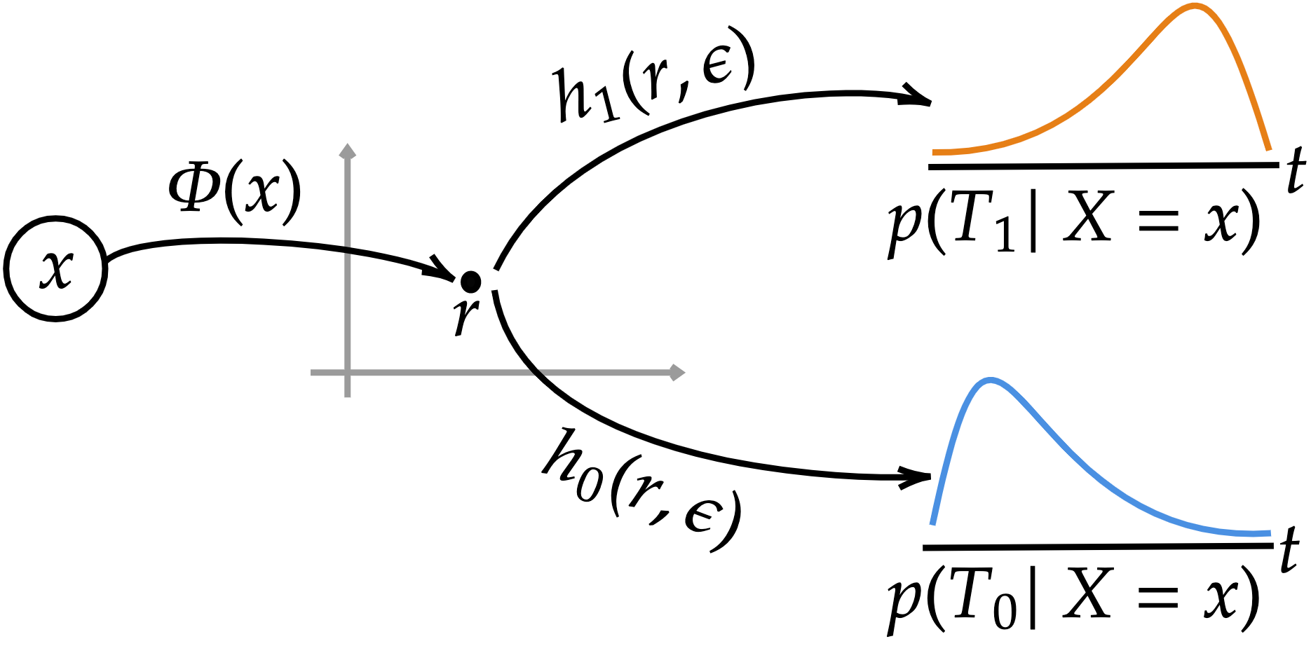
In this work, we are interested in the expected difference between the $T_{1}$ and $T_{0}$ conditioned on $X$ for a given unit (individual), which is commonly known as the individualized treatment effect (ITE). Specifically, we wish to perform inference on the conditional distributions of $T_{1}$ and $T_{0}$, i.e., $p(T_{1}|X)$ and $p(T_{0}|X)$, respectively, as shown in Figure 1(a). In practice, we observe $N$ realizations of $(Y,\delta,X,A)$ for observed time, censoring indicator, covariates and treatment indicator, respectively; hence, from an observational study the dataset takes the form $\mathcal{D}=\{(y_{i},\delta_{i},{x}_{i},a_{i})\}_{i=1}^{N}$. Below, we discuss several common choices of estimands in survival analysis.

(a) Counterfactual inference

(b) Non-informative

(c) Informative

Figure 1. (a) Illustration of the proposed counterfactual survival analysis (CSA). Covariates $X=x$ are mapped into latent representation $r$ via deterministic mapping $r=\Phi(x)$. The potential outcomes are sampled from $t_{a}\sim p(T_{A}|X=x)$ for $A=a$ via stochastic mapping $h_{A}({r},\tilde{\epsilon})$, where stochasticity is induced with a planar-flow-based transformation, $\tilde{\epsilon}$, of a simple distribution $p(\epsilon)$, i.e., uniform or Gaussian. (b) and (c) show the proposed causal graphs for non-informative and informative censoring, respectively.

2.1. Estimands of Interest

We begin by considering survival analysis in the absence of an intervening treatment choice, $A$. Let $F(t|x)\triangleq P(T\leq t|X=x)$ be the cumulative distribution function of the event (failure) time, $t$, given a realization of the covariates, $x$. Survival analysis is primarily concerned with characterization of the survival function conditioned on covariates $S(t|x)\triangleq 1-F(t|x)$, and the hazard function or risk score, $\lambda(t|x)$, defined below. $S(t|x)$ is a monotonically decreasing function indicating the probability of survival up to time $t$. The hazard function measures the instantaneous probability of the event occurring between $\{t,t+\Delta t\}$ given $T>t$ and $\Delta t\to 0$. From standard definitions (Kleinbaum and Klein, 2010), the relationship between cumulative and hazard function is formulated as

(1) $$\begin{aligned} \lambda(t|x)&=\lim\limits_{dt\rightarrow 0}\frac{P(t<T<t+dt|X=x)}{P(T>t|X=x)dt}\\ &=-\frac{d\log S(t|x)}{dt}=\frac{f(t|x)}{S(t|x)}.\end{aligned}$$

From (1) we see that $f(t|x)\triangleq P(T=t|X=x)=\lambda(t|x)S(t|x)$, is the conditional event time density function (Kleinbaum and Klein, 2010).

Given the binary treatment $A$, we are interested in its impact on the survival time. For ITE estimation, we are also interested in the difference between the two potential outcomes $T_{1},T_{0}$. Let $S_{A}(t|x)$ and $\lambda_{A}(t|x)$ denote the survival and hazard functions for the potential outcomes $T_{A}$, i.e., $T_{1}$ and $T_{0}$. Several common estimands of interest include (Zhao et al., 2012; Trinquart et al., 2016):

• Difference in expected lifetime:
  $\textup{ITE}(x)=\int_{0}^{t_{\max}}\{S_{1}(t|x)-S_{0}(t|x)\}\textup{d}t=\mathbb{E}\{T_{1}-T_{0}|X=x\}$.

• Difference in survival function: $\textup{ITE}(t,x)=S_{1}(t|x)-S_{0}(t|x)$.

• Hazard ratio: $\textup{ITE}(t,x)=\lambda_{1}(t|x)/\lambda_{0}(t|x)$.

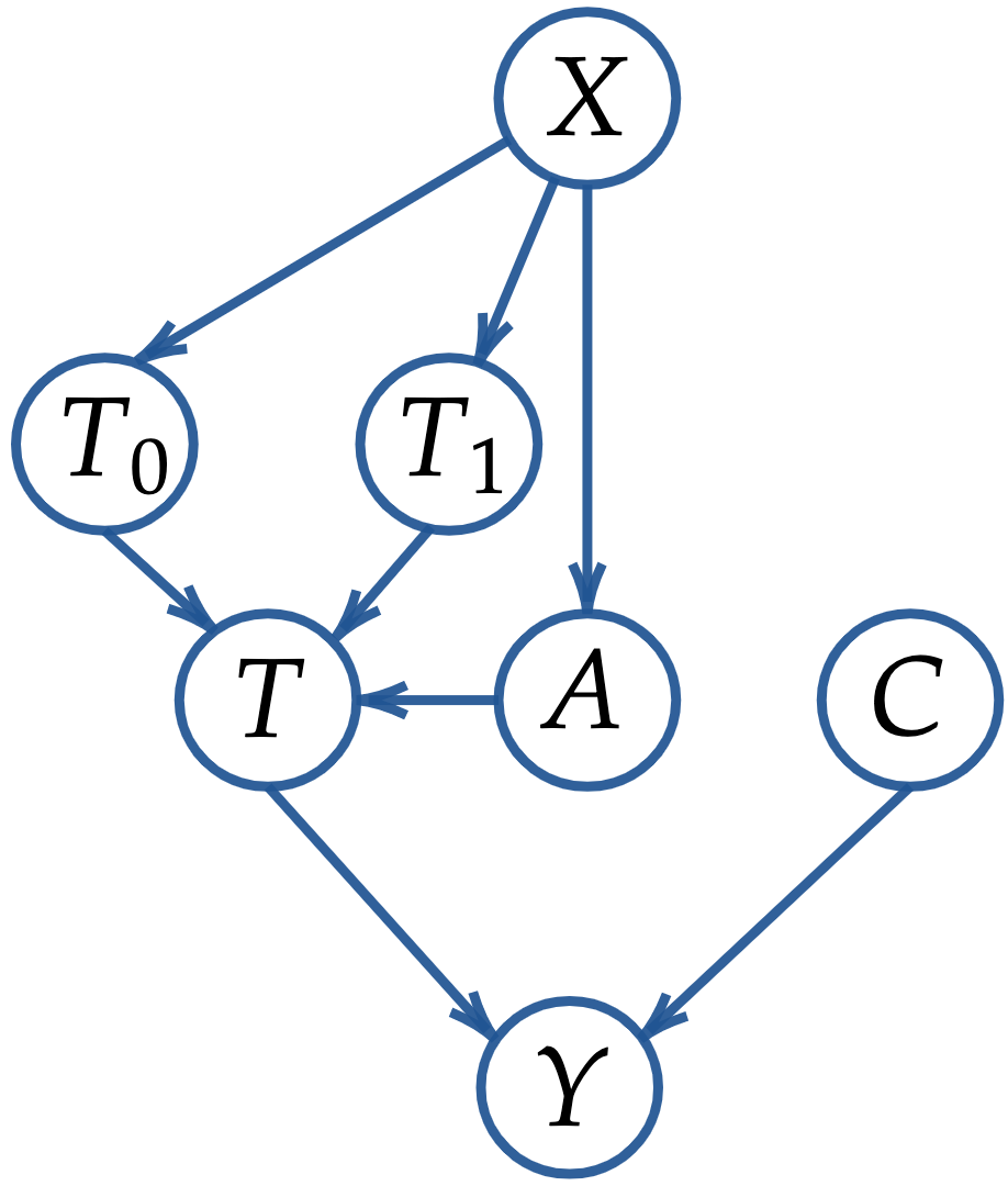
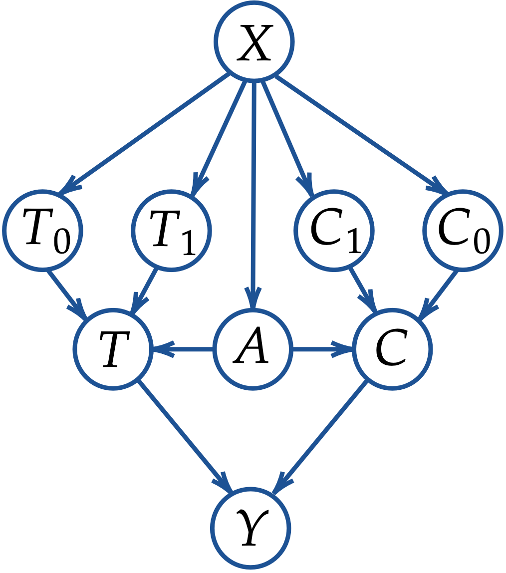
The inference difficulties associated with the above estimands from observational data are two-fold. First, there are confounders affecting both the treatment assignment and outcomes, which stem from selection bias, i.e., the treatment and control covariate distributions are not necessarily the same. Also, we do not have direct knowledge of the conditional treatment assignment mechanism, i.e., $P(A=a|X=x)$, also known as the propensity score. Let $\mathrel{\text{\scalebox{1.07}{$\perp\mkern-10.0mu\perp$}}}$ denote statistical independence. For estimands to be identifiable from observational data, we make two assumptions: ($i$) $\{T_{1},T_{0}\}\mathrel{\text{\scalebox{1.07}{$\perp\mkern-10.0mu\perp$}}}A|X$, i.e., no unobserved confounders or ignorability, and ($ii$) overlap in the covariate support $0<P(A=1|X=x)<1$ almost surely if $p(X=x)>0$. Second, the censoring mechanism is also unknown and may lead to bias without proper adjustment. We consider two censoring mechanisms in our work, ($i$) conditionally independent or informative censoring: $T\mathrel{\text{\scalebox{1.07}{$\perp\mkern-10.0mu\perp$}}}C|X,A$, and ($ii$) random or non-informative censoring: $T\mathrel{\text{\scalebox{1.07}{$\perp\mkern-10.0mu\perp$}}}C$. Note that for informative censoring, we also have to consider potential censoring times $C_{1}$ and $C_{0}$ and their conditionals $p(C_{1}|X)$ and $p(C_{0}|X)$, respectively. Figure 1 shows causal graphs illustrating these modeling assumptions.

3. Modeling

To overcome the above challenges and adjust for observational biases, we propose a unified framework for counterfactual survival analysis (CSA). Specifically, we repurpose the counterfactual bound in Shalit et al. (2017) for our time-to-event scenario and introduce a nonparametric approach for stochastic survival outcome predictions. Below we formulate a theoretically grounded and unified approach for estimating $(i)$ the encoder function ${r}=\Phi(x)$, which deterministically maps covariates $x$ to their corresponding latent representation ${r}\in\mathbb{R}^{d}$, and $(ii)$ two stochastic time-to-event generative functions, $h_{A}(\cdot)$, to implicitly draw samples from both potential outcome conditionals $t_{a}\sim p_{h,\Phi}(T_{A}|X=x)$, for $A=\{1,0\}$, and where $t_{a}$ indicates the sample from $p_{h,\Phi}(T_{A}|X=x)$ is for $A=a$. Further, we formulate a general extension that accounts for informative censoring by introducing two stochastic censoring generative functions, $\nu_{A}(\cdot)$, to draw samples for potential censoring times $c_{a}\sim p_{\nu,\Phi}(C_{A}|X=x)$. The model-specifying functions, $\{h_{A}(\cdot),\nu_{A}(\cdot),\Phi(\cdot)\}$, are parameterized via neural networks. See the Supplementary Material (SM) for details. Figure 1(a) summarizes our modeling approach.

3.1. Accounting for selection bias

We wish to estimate the potential outcomes, i.e., event times, which are sampled by distributions parameterized by functions $\{h_{A}(\cdot),\Phi(\cdot)\}$, i.e.,

(2) $$t \sim p_{h,\Phi}(T|X=x,A=a)$$

(3) $$t_{a} \sim p_{h,\Phi}(T_{a}|X=x)$$

We obtain (3) from (2) via the strong ignorability assumption, i.e., $\{T_{0},T_{1}\}\mathrel{\text{\scalebox{1.07}{$\perp\mkern-10.0mu\perp$}}}A|X$ (consistent with the causal graphs in Figure 1(b) and 1(c)) and $0<P(A=a|X=x)<1$, and the consistency assumption, i.e., $T=T_{A}|A=a$. A similar argument can be made for informative censoring based on Figure 1(c), so we can also write $c_{a}\sim p_{\nu,\Phi}(C_{A}|X=x)$. Given (3), model functions $\{h_{A}(\cdot),\Phi(\cdot)\}$ and $\nu_{A}(\cdot)$ for informative censoring can be learned by leveraging standard statistical optimization approaches, that minimize a loss hypothesis $\mathcal{L}$ given samples from the empirical distribution $(y,\delta,x,a)\sim p(Y,\delta,X,A)$, i.e., from dataset $\mathcal{D}$. Specifically, we write $\mathcal{L}$ as

(4) $$\mathcal{L} =\mathbb{E}_{(y,\delta,x,a)\sim p(Y,\delta,X,A)}\left[\ell_{h,\Phi}(t_{a},y,\delta)\right]\,,$$

where $\ell_{h,\Phi}(t_{a},y,\delta)$ is a loss function that measures the agreement of $t_{a}\sim p_{h,\Phi}(T_{A}|X=x)$ (and $c_{a}\sim p_{\nu,\Phi}(C_{A}|X=x)$ for informative censoring) with ground truth $\{y,\delta\}$, the observed time and censoring indicator, respectively.

For some parametric formulations of event time distribution $p_{h,\Phi}(T_{A}|X=x)$, e.g., exponential, Weibull, log-Normal, etc., and provided the censoring mechanism is non-informative, $-\ell_{h,\Phi}(t_{a},y,\delta)$ is the closed form log likelihood. Specifically, $-\ell_{h,\Phi}(t_{a},y,\delta)\triangleq\log p_{h,\Phi}(T_{a}|X=x)=\delta\cdot\log f_{h,\Phi}(t_{a}|x)+(1-\delta)\cdot\log S_{h,\Phi}(t_{a}|x)$, which implies that the conditional event time density and survival functions can be calculated in closed form from transformations $\{h_{A}(\cdot),\Phi(\cdot)\}$ of $x$. See the SM for parametric examples of (4) accounting for informative censoring.

We further define the expected loss for a given realization of covariates $x$ and treatment assignment $a$ over observed times $y$ (censored and non-censored), and the censoring indicator $\delta$ as $\zeta_{h,\Phi}(x,a)\triangleq\mathbb{E}_{(y,\delta,x)\sim p(Y,\delta|X)}\ell_{h,\Phi}(t_{a},y,\delta)$ as in Shalit et al. (2017). For a given subject with covariates $x$ and treatment assignment $a$, we wish to minimize both the factual and counterfactual losses, $\mathcal{L}_{\rm F}$ and $\mathcal{L}_{\rm CF}$, respectively, by decomposing $\mathcal{L}=\mathcal{L}_{\rm F}+\mathcal{L}_{\rm CF}$ as follows

(5) $$\begin{aligned} \mathcal{L}_{\rm F}&=\mathbb{E}_{(x,a)\sim p(A,X)}\zeta_{h,\Phi}(x,a)\,,\\ \mathcal{L}_{\rm CF}&=\mathbb{E}_{(x,a)\sim p(1-A,X)}\zeta_{h,\Phi}(x,a)\,.\end{aligned}$$

Let $u\triangleq P(A=1)$ denote the marginal probability of treatment assignment. We can readily decompose the losses in (5) according to treatment assignments. The decomposed factual $\mathcal{L}_{\rm F}=u\cdot\mathcal{L}_{\rm F}^{A=1}+(1-u)\cdot\mathcal{L}_{\rm F}^{A=0}$, and similarly, the decomposed counterfactual $\mathcal{L}_{\rm CF}=(1-u)\cdot\mathcal{L}_{\rm CF}^{A=1}+u\cdot\mathcal{L}_{\rm CF}^{A=0}$. In practice, only factual outcomes are observed, hence, for a non-randomized non-controlled experiment, we cannot obtain an unbiased estimate of $\mathcal{L}_{\rm CF}$ from data due to selection bias (or confounding). Therefore, we bound $\mathcal{L}_{\rm CF}$ and $\mathcal{L}$ below following Shalit et al. (2017).

Corollary 0.

Assume  $\Phi(\cdot)$ is an invertible map, and  $\alpha^{-1}\zeta_{h,\Phi}(x,a)\in G$, where $G$ is a family of functions, $p_{\Phi}^{A=a}\triangleq p_{\Phi}(R|A=a)$ is the latent distribution for group $A=a$, and $\alpha>0$ is a constant. Then, we have:

$$\mathcal{L}_{\rm CF} \leq(1-u)\cdot\mathcal{L}_{\rm F}^{A=1}+u\cdot\mathcal{L}_{\rm F}^{A=0}+\alpha\cdot{\rm IPM}_{G}(p_{\Phi}^{A=1},p_{\Phi}^{A=0})$$

(6) $$\mathcal{L} \leq\mathcal{L}_{\rm F}^{A=1}+\mathcal{L}_{\rm F}^{A=0}+\alpha\cdot{\rm IPM}_{G}(p_{\Phi}^{A=1},p_{\Phi}^{A=0})\,.$$

The integral probability metric (IPM) (Müller, 1997; Sriperumbudur et al., 2012) measures the distance between two probability distributions $p$ and $q$ defined over $M$, i.e., the latent space of $R$. Formally,
${\rm IPM}_{G}(p,q)\triangleq\sup_{g\in G}|\int_{M}g(m)\left(p(m)-q(m)\right)dm|$, where $g:m\rightarrow\mathbb{R}$, represents a class of real-valued bounded measurable functions on $M$ (Shalit et al., 2017). Therefore, model functions $\{h_{a}(\cdot),\Phi(\cdot)\}$ can be learned by minimizing the upper bound in (6) consisting of $(i)$ only factual losses under both treatment assignments and $(ii)$ an IPM regularizer enforcing latent distributional equivalence between the treatment groups. Note that if the data originates from a RCT it follows (by construction) that ${\rm IPM}_{G}(p_{\Phi}^{A=1},p_{\Phi}^{A=0})=0$.

3.2. Accounting for censoring bias

Below we formulate an approach for estimating functions $h_{A}(\cdot)$ and $\nu_{A}(\cdot)$ for synthesizing (sampling) non-censored $t_{a}\sim p_{h,\Phi}(T_{A}|X=x)$ and censored $c_{a}\sim p_{\nu,\Phi}(C_{A}|X=x)$ times, respectively. While some parametric assumptions for $p_{h,\Phi}(T_{A}|X=x)$ yield easy-to-evaluate closed forms for $S_{h,\Phi}(t_{a}|x)$ that can be used as likelihood for censored observations, they are restrictive, and have been shown to generate unrealistic high variance samples (Chapfuwa et al., 2018). So motivated, we seek a nonparametric likelihood-based approach that can model a flexible family of distributions, with an easy-to-sample approach for event times $t_{a}\sim p_{h,\Phi}(T_{a}|X=x)$. We model the event time generation process with a source of randomness, $p({\epsilon})$, e.g. Gaussian or uniform, which is obtained from a neural-network-based nonlinear transformation. In the experiments we use a planar flow formulation parameterized by $\{U_{h},W_{h},b_{h}\}$ (Rezende and Mohamed, 2015), however, other specifications can also be used. Note that (Miscouridou et al., 2018) has previously leveraged normalizing flows for survival analysis, however, our approach is very different in that it focuses on $i$) formulating a counterfactual survival analysis framework that accounts for informative or non-informative censoring mechanisms and confounding, and $ii$) modeling event times as a continuous variable instead of discretizing them. Specifically, we transform the source of randomness, $\epsilon$, using a single layer specification as follows

(7) $$\begin{aligned} \tilde{\epsilon}_{h}&={\epsilon}+{U}_{h}\tanh(W_{h}\epsilon+b_{h})\,,\quad\epsilon\sim{\rm Uniform}(0,1)\,,\\ t_{a}&=h_{A}({r},\tilde{\epsilon}_{h})\,,\quad{r}=\Phi(x)\end{aligned}$$

where $\{U_{h},W_{h}\}\in\mathbb{R}^{d\times d}$, $\{b_{h},\epsilon\}\in\mathbb{R}^{d}$, $d$ is the dimensionality of the planar flow; each component of $\epsilon$ is drawn independently from ${\rm Uniform}(0,1)$, and $\tilde{\epsilon}_{h}$ may be viewed as a skip connection with stochasticity in $\epsilon$. Further, $h_{A}(r,\tilde{\epsilon}_{h})$ and $\Phi(x)$ are time-to-event generative and encoding functions, respectively, parameterized as neural networks. For simplicity, the dimensions of ${r}$ and $\epsilon$ are set to $d$, however, they can be set independently if desired. In practice, we are interested in generating realistic event-time samples; therefore, we account for both censored and non-censored observations by adopting the objective from Chapfuwa et al. (2018), formulated as

(8) $$\begin{aligned} \mathcal{L}_{\rm F}^{\rm CSA}&\triangleq\mathbb{E}_{(y,\delta,x,a)\sim p(Y,\delta,X,A),\epsilon\sim p(\epsilon)}\left[\delta\cdot\left(|y-t_{a}|\right)\right.\\ &+\left.(1-\delta)\cdot\left(\max(0,y-t_{a})\right)\right]\,,\end{aligned}$$

where the first term encourages sampled event times $t_{a}$ to be close to $y$, the ground truth for observed events, i.e., $\delta=1$, while penalizing $t_{a}$ for being smaller than the censoring time when $\delta=0$. Further, the expectation is taken over samples (a minibatch) from empirical distribution $p(Y,\delta,X,A)$.

Informative censoring

We model informative censoring similar to (8) but mirroring the censoring indicators to encourage accurate censoring time samples $c_{a}$ for $\delta=0$, while penalizing $c_{a}$ for being smaller than $y$ for $\delta=1$ (observed events). Specifically, we set an independent source of randomness like in (7) but parameterized by $\{{U}_{\nu},{W}_{\nu},b_{\nu}\}$ and censoring generative functions $\nu_{A}({r},\tilde{\epsilon}_{\nu})$, parameterized as neural networks, where $c_{a}\sim p_{\nu,\Phi}(C_{A}|X=x)$ formulated as

(9) $$\begin{aligned} \ell_{c}(\nu,\Phi)&=\mathbb{E}_{(y,\delta,x,a)\sim p(y,\delta,X,A),\boldsymbol{\epsilon}\sim p(\epsilon)}\left[(1-\delta)\cdot\left(|y-c_{a}|\right)\right.\\ &+\left.\delta\cdot\left(\max(0,y-c_{a})\right)\right]\,.\end{aligned}$$

Further, we introduce an additional time-order-consistency loss that enforces the correct order of the observed time relative to the censoring indicator, i.e., $c_{a}<t_{a}$ if $\delta=0$ and $t_{a}<c_{a}$ if $\delta=1$, thus

(10) $$\begin{aligned} \ell_{\rm TC}(h,\nu,\Phi)&=\mathbb{E}_{(\delta,x,a)\sim p(\delta,X,A),\epsilon\sim p(\epsilon)}\left[\delta\cdot\left(\max(0,t_{a}-c_{a})\right)\right.\\ &+\left.(1-\delta)\cdot\left(\max(0,c_{a}-t_{a})\right)\right]\,.\end{aligned}$$

Note that $\ell_{\rm TC}(h,\nu,\Phi)$ does not depend on the observed event times but only on the censoring indicators. Finally, we write the consolidated CSA loss for informative censoring (CSA-INFO) by aggregating (8), (9) and (10) as

(11) $$\mathcal{L}_{\rm F}^{\rm CSA-INFO} \triangleq\mathcal{L}_{\rm F}^{\rm CSA}+\ell_{\rm c}+\ell_{\rm TC}\,.$$

Table 1. Performance comparisons on actg-Synthetic data, with 95% ${\rm HR}(t)$ confidence interval. The ground truth, test set, hazard ratio is $\rm{HR(t)}=0.52_{(0.39,0.71)}$.

Method Causal metrics Factual metrics $\epsilon_{\rm PEHE}$ $\epsilon_{\rm ATE}$ ${\rm HR}(t)$ C-Index (A=0, A=1) Mean COV C-Slope (A=0, A=1) CoxPH-Uniform NA NA $0.97_{(0.86,1.09)}$ NA NA NA CoxPH-IPW NA NA $0.48_{(0.03,7.21)}$ NA NA NA CoxPH-OW NA NA $0.60_{(0.53,0.68)}$ NA NA NA Surv-BART 352.07 77.89 $0.0(0.0,0.0)$ (0.706, 0.686) 0.001 (0.398, $\infty$) AFT-Weibull 367.92 133.93 $0.47_{(0.47,0.47)}$ (0.21, 0.267) 6.209 (0.707, 0.729) AFT-log-Normal 377.76 157.64 $0.47_{(0.47,0.47)}$ (0.675, 0.556) 6.971 (0.707, 0.729) SR 369.47 88.55 $0.38_{(0.33,0.65)}$ (0.791, 0.744) 0 (0.985, 1.027) CSA (proposed) 358.72 0.8 $0.45_{(0.39,0.65)}$ (0.787, 0.767) 0.131 (0.985, 1.026) CSA-INFO (proposed) 344.3 31.19 $\textbf{0.53}_{(0.41,0.67)}$ (0.78, 0.764) 0.13 (0.999, 1.029)

3.3. Learning

Model functions $\{h_{A}(\cdot),\Phi(\cdot),\nu_{A}(\cdot)\}$ are learned by minimizing the bound (6), via stochastic gradient descent on minibatches from $\mathcal{D}$, with $\mathcal{L}_{\rm F}^{\rm CSA}$ for non-informative censoring and $\mathcal{L}_{\rm F}^{\rm CSA-INFO}$ for informative censoring. Further, for the ${\rm IPM}$ regularization loss in (6), we optimize the dual formulation of the Wasserstein distance, via the regularized optimal transport (Villani, 2008; Cuturi, 2013). Consequently, we only require $\alpha^{-1}\zeta_{h,\Phi}(x,a)$ to be $1$-Lipschitz (Shalit et al., 2017) and $\alpha$ is selected by grid search on the validation set using only factual data (details below).

4. Metrics

We propose a comprehensive evaluation approach that accounts for both factual and causal metrics. Factual survival outcome predictions are evaluated according to standard survival metrics that measure diverse performance characteristics, such as concordance index (C-Index) (Harrell Jr et al., 1984), mean coefficient of variation (COV) and calibration slope (C-slope) (Chapfuwa et al., 2020). See the SM for more details on these metrics. For causal metrics, defined below, we introduce a nonparametric hazard ratio (HR) between treatment outcomes, and adopt the conventional precision in estimation of heterogeneous effect (PEHE) and average treatment effect (ATE) performance metrics (Hill, 2011). Note that PEHE and ATE require ground truth counterfactual event times, which is only possible for (semi-)synthetic data. For HR, we compare our findings with those independently reported in the literature from gold-standard RCT data.

Table 2. Performance comparisons on Framingham data, with 95% ${\rm HR}(t)$ confidence interval. Test set NN assignment of $y_{\rm{CF}}$ and $\delta_{\rm{CF}}$ yields biased ${\rm HR(t)}=1.23_{(1.17,1.25)}$, while previous large scale longitudinal RCT studies estimated ${\rm HR(t)}=0.75_{(0.64,0.88)}$ (Yusuf et al., 2016).

Method Causal metric Factual metrics ${\rm HR}(t)$ C-Index (A=0, A=1) Mean COV C-Slope (A=0, A=1) CoxPH-Uniform $1.69_{(1.38,2.07)}$ NA NA NA CoxPH-IPW $1.09_{(0.76,1.57)}$ NA NA NA CoxPH-OW $0.88_{(0.73,1.08)}$ NA NA NA Surv-BART $14.99_{(14.9,14.9e8)}$ (0.629, 0.630) 0.003 (0.232, 0.084) AFT-Weibull $1.09_{(1.09,1.09)}$ (0.734, 0.395) 8.609 (0.857, 0.89) AFT-log-Normal $1.55_{(1.46,1.55)}$ (0.68, 0.56) 10.415 (0.979, 0.732) SR $0.58_{(0.53,0.71)}$ (0.601, 0.57) 0 (0.491, 0.63) CSA (proposed) $1.04_{(1.00,1.09)}$ (0.763, 0.728) 0.161 (0.891, 0.81) CSA-INFO (proposed) $\textbf{0.81}_{(0.77,0.83)}$ (0.752, 0.651) 0.156 (0.907, 0.881)

Nonparametric Hazard Ratio

In medical settings, the population hazard ratio ${\rm HR}(t)$ between treatment groups is considered informative thus has been widely used in drug development and RCTs (Yusuf et al., 2016; Mihaylova et al., 2012). For example, ${\rm HR}(t)<1$, $>1$, or $\approx 1$ indicate population positive, negative and neutral treatment effects at time $t$, respectively. Moreover, ${\rm HR}(t)$ naturally accounts for both censored and non-censored outcomes. Standard approaches for computing ${\rm HR}(t)$ rely on the restrictive proportional hazard assumption from CoxPH (Cox, 1972), which is constituted as a semi-parametric linear model $\lambda(t|a)=\lambda_{\rm b}(t)\exp(a\beta)$. However, the constant covariate (time independent) effect is often violated in practice (see Figure 2(b)). For CoxPH, the marginal HR between treatment and control can be obtained from regression coefficient $\beta$ learned via maximum likelihood without the need for specifying the baseline hazard $\lambda_{\rm b}(t)$:

(12) $${\rm HR}_{\rm CoxPH}(t) =\frac{\lambda(t|a=1)}{\lambda(t|a=0)}=\exp(\beta)\,.$$

So motivated, we propose a nonparametric, model-free approach for computing ${\rm HR}(t)$, in which we do not assume a parametric form for the event time distribution or the proportional hazard assumption from CoxPH. This approach only relies on samples from the conditional event time density functions, $f(t_{1}|x)$ and $f(t_{0}|x)$, via $t_{a}=h_{A}(\cdot)$ from (7).

Definition 0.

We define the nonparametric marginal Hazard Ratio and its approximation, ${\rm\hat{HR}}(t)$, as

where for ${\rm HR}(t)$ we leveraged (1) to obtain (1) and $S^{\prime}(t)\triangleq dS(t)/dt$. The nonparametric assumption for $S(t)$ makes the computation of $S^{\prime}(t)$ challenging. Provided that $S(t)$ is a monotonically decreasing function, for simplicity, we fit a linear function $S(t)=m\cdot t+c$, and set $S^{\prime}(t)\approx m$. Note that the linear model is only used for estimating $S^{\prime}(t)$ from the nonparametric estimation of $S(t)$. Bias from $S^{\prime}(t)$ can be reduced by considering more complex function approximations for $S(t)$, e.g., polynomial or spline. For the nonparametric estimation of $S(t)$ we leverage the model-free population point-estimate-based nonparametric Kaplan-Meier (Kaplan and Meier, 1958) estimator of the survival function $\hat{S}^{\rm PKM}(t)$ in (Chapfuwa et al., 2020) to marginalize both factual and counterfactual predictions given covariates $x$. The approximated hazard ratio, ${\rm\hat{HR}}(t)$, is thus obtained by combining the approximations $\hat{S}^{\rm PKM}_{a}(t)$ and $m_{a}$. A similar formulation for the conditional, ${\rm\hat{HR}}(t|x)$, can also be derived. See the SM for full details on the evaluation of ${\rm\hat{HR}}(t)$ and ${\rm\hat{HR}}(t|x)$. Note that for some AFT- or CoxPH-based parametric formulations, ${\rm HR}(t|x)$, can be readily evaluated because $f(t_{a}|x)$ and $S(t_{a}|x)$ are available in closed form.

In the experiments, we will use ${\rm HR}(t)$ to compare different approaches against results reported in RCTs (see Tables 1 and 2). Further, we will use ${\rm HR}(t|x)$ to illustrate stratified treatment effects (see Figure 2). Note that though a neural-network-based survival recommender system (Katzman et al., 2018) has been previously used to estimate ${\rm HR}(t|x)$, their approach does not account for confounding or informative censoring thus it is susceptible to bias.

Precision in Estimation of Heterogeneous Effect (PEHE)

A general individualized estimation error is formulated as

$$\epsilon_{\rm PEHE}=\sqrt{\mathbb{E}_{X}[({\rm ITE}(x)-\hat{\rm ITE}(x))^{2}]},$$

where ${\rm ITE}(x)$ is the ground truth, $\hat{\rm ITE}(x)=\mathbb{E}_{T}\left[\gamma\left(T_{1}\right)-\gamma\left(T_{0}\right)|X=x\right]$ and $\gamma(\cdot)$ is a deterministic transformation. In our experiments, $\gamma(\cdot)$ is the average over samples from $t_{a}\sim p_{h,\Phi}(T_{A}|X=x)$. Alternative estimands, e.g., thresholding survival times $\gamma(T_{A})=I\{T_{A}>\tau\}$, can also be considered as described in Section 2.1.

Average Treatment Effect (ATE)

The population treatment effect estimation error is defined as

$$\epsilon_{\rm ATE}=|{\rm ATE}-\hat{\rm ATE}|,$$

where ${\rm ATE}=\mathbb{E}_{X}[{\rm ITE}(x)]$ (ground truth) and $\hat{\rm ATE}=\mathbb{E}_{X}[\hat{\rm ITE}(x)]$.

Note that both PEHE and ATE require ground truth (population and individual) treatment effects to be available, which is only possible in synthetic and semi-synthetic data (benchmarking) scenarios.

5. Experiments

We describe the baselines and datasets that will be used to evaluate the proposed counterfactual survival analysis methods (CSA and CSA-INFO). Detailed architecture information of the proposed methods (CSA and CSA-INFO) and baselines (AFT-log-Normal, AFT-Weibull, Semi-supervised Regression(SR)) are provided in the SM. Pytorch code to replicate experiments can be found at https://github.com/paidamoyo/counterfactual_survival_analysis. Throughout the experiments, we use the standard ${\rm HR}(t)$ for CoxPH based methods in (12) and (1) for all others. The bound in (6) is sensitive to $\alpha$, thus we propose approximating proxy counterfactual outcomes $\{Y_{\rm CF},\delta_{\rm CF}\}$ for the validation set, according to the covariate Euclidean nearest-neighbour (NN) from the training set. We select the $\alpha$ that minimizes the validation loss $\mathcal{L}=\mathcal{L}_{\rm F}+\mathcal{L}_{\rm CF}$ from the set $(0,0.1,1,10,100)$.

Baselines

We consider the following competitive baseline approaches: $(i)$ propensity weighted CoxPH (Schemper et al., 2009; Buchanan et al., 2014; Rosenbaum and Rubin, 1983); $(ii)$ ${\rm IPM}$ (6) regularized AFT (log-Normal and Weibull) models; $(iii)$ an ${\rm IPM}$ (6) regularized deterministic semi-supervised regression (SR) model with accuracy objective from (Chapfuwa et al., 2018), as a contrast for the proposed stochastic predictors (CSA and CSA-INFO); and $(iv)$ survival Bayesian additive regression trees (Surv-BART) (Sparapani et al., 2016). For CoxPH, we consider three normalized weighting schemes: $(i)$ inverse probability weighting (IPW) (Horvitz and Thompson, 1952; Cao et al., 2009), where ${\rm IPW}_{i}=\frac{a_{i}}{\hat{e}_{i}}+\frac{1-a_{i}}{1-\hat{e}_{i}}$; $ii)$ overlapping weights (OW) (Crump et al., 2006; Li et al., 2018), where ${\rm OW}_{i}=a_{i}\cdot(1-\hat{e}_{i})+(1-a_{i})\cdot\hat{e}_{i}$; and $iii)$ the standard RCT uniform assumption. A simple linear logistic model $\hat{e}_{i}=\sigma(x_{i};w)$, is used as an approximation, $\hat{e}_{i}$, to the unknown propensity score $P(A=1|X=x)$. See the SM for more details of the baselines.

(a) actg-synthentic ${\rm HR}(t)$

(b) Framingham $\log{\rm HR}(t|x)$

(c) Framingham $\log{\rm HR}(t|x)$ pdf

Figure 2. (a) Inferred population ${\rm HR}(t)$ compared against ground truth (EMP) on actg-Synthetic data. CSA-INFO-based (b) cluster-specific average $\log{\rm HR}(t|x)$ curves and (c) estimated density of median $\log{\rm HR}(t|x)$ values on the test set of the Framingham dataset. Clusters assignment were obtained via hierarchical clustering of individualized $\log{\rm HR}(t|x)$ traces.

Datasets

We consider the following datasets summarized in Table 3: $(i)$ Framingham, is an EHR-based longitudinal cardiovascular cohort study that we use to evaluate the effect of statins on future coronary heart disease outcomes (Benjamin et al., 1994); $(ii)$ actg, is a longitudinal RCT study comparing monotherapy with Zidovudine or Didanosine with combination therapy in HIV patients (Hammer et al., 1996); and $(iii)$ actg-Synthetic, is a semi-synthetic dataset based on actg covariates. We simulate potential outcomes according to a Gompertz-Cox distribution (Bender et al., 2005) with selection bias from a simple logistic model for $P(A=1|X=x)$ and AFT-based censoring mechanism. The generative process is detailed in the SM. Table 3 summarizes the datasets according to $(i)$ covariates of size $p$; $(ii)$ proportion of non-censored events, treated units, and missing entries in the $N\times p$ covariate matrix; and $(iii)$ time range $t_{\rm max}$ for both censored and non-censored events. Missing entries are imputed with the median or mode if continuous or categorical, respectively.

Table 3. Summary statistics of the datasets.

	Framingham	actg	actg-synthetic
Events (%)	26.0	26.9	48.9
Treatment (%)	10.4	49.5	55.9
$N$	3,435	1,054	2,139
$p$	32	23	23
Missing (%)	0.23	1.41	1.38
$t_{\rm max}$ (days)	7,279	1,231	1,313

Quantitative Results

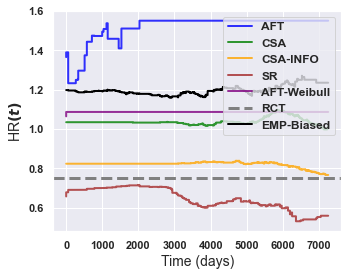
Experimental results for two data-sets in Tables 1 and 2, illustrate that AFT-based methods have high variance, inferior in calibration and C-Index than accuracy-based methods (SR, CSA, CSA-INFO). Surv-BART is the least calibrated but low variance method. CSA-INFO and CSA outperform all methods across all factual metrics, whereas CSA-INFO is better calibrated, has low variance but slightly lower C-Index than CSA. Note that we fit CoxPH using the entire dataset; since it does not support counterfactual inference, we do not present factual metrics. By properly adjusting for both informative censoring and selection bias, CSA-INFO significantly outperforms all methods in treatment effect estimation according to ${\rm HR}(t)$ and $\boldsymbol{\epsilon}_{\rm PEHE}$, across non-RCT datasets, while remaining comparable to AFT-Weibull on the RCT dataset (see the SM). Further, RCT-based results on actg data in the SM illustrate comparable ${\rm HR}(t)$ across all models except for AFT-log-Normal and Surv-BART, which overestimate, and SR, which underestimates risk. For non-RCT datasets (actg-Synthentic and framingham), CoxPH-OW has a clear advantage over all CoxPH based methods, mostly credited to the well-behaved bounded propensity weights $\in[0,1]$. Interestingly, the Framingham observational data exhibits a common paradox, where without proper adjustment of selection and censoring bias, naive approaches would result in a counter-intuitive treatment effect from statins. However, there is severe confounding from covariates such as age, BMI, diabetes, CAD, PAD, MI, stroke, etc., that influence both treatment likelihood and survival time. Table 2, demonstrates that CSA-INFO is clearly the best performing approach. Specifically, its ${\rm HR}(t)$, reverses the biased observational treatment effect, to demonstrate positive treatment from statins, which is consistent with prior large RCT longitudinal findings (Yusuf et al., 2016). Consequently, our experiments are comprehensive and we are confident that the CSA-INFO performance benefits are attributed to $(i)$ accounting for informative censoring bias; $(ii)$ accounting for selection bias (optimal IPM regularizer with $\alpha>0$); and $(iii)$ flexible and non-parametric generative modeling of event times from the stochastic planar flow.

Qualitative Results

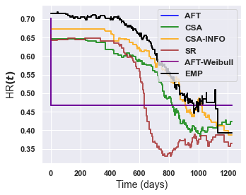
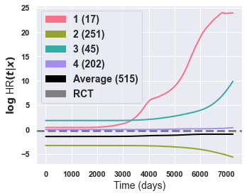
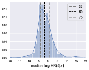
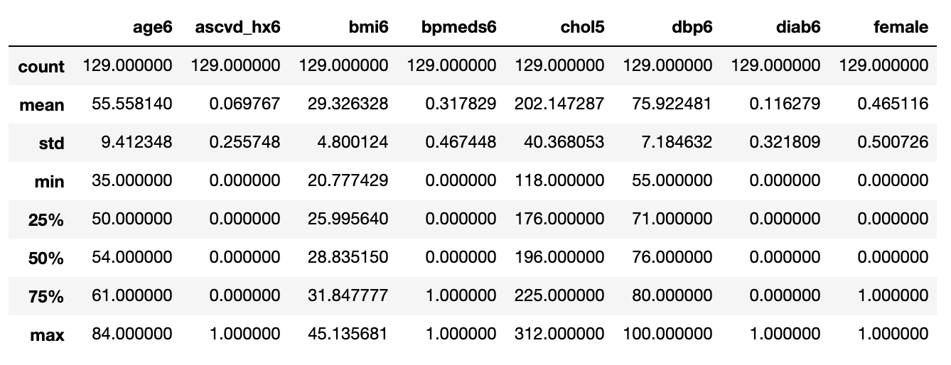
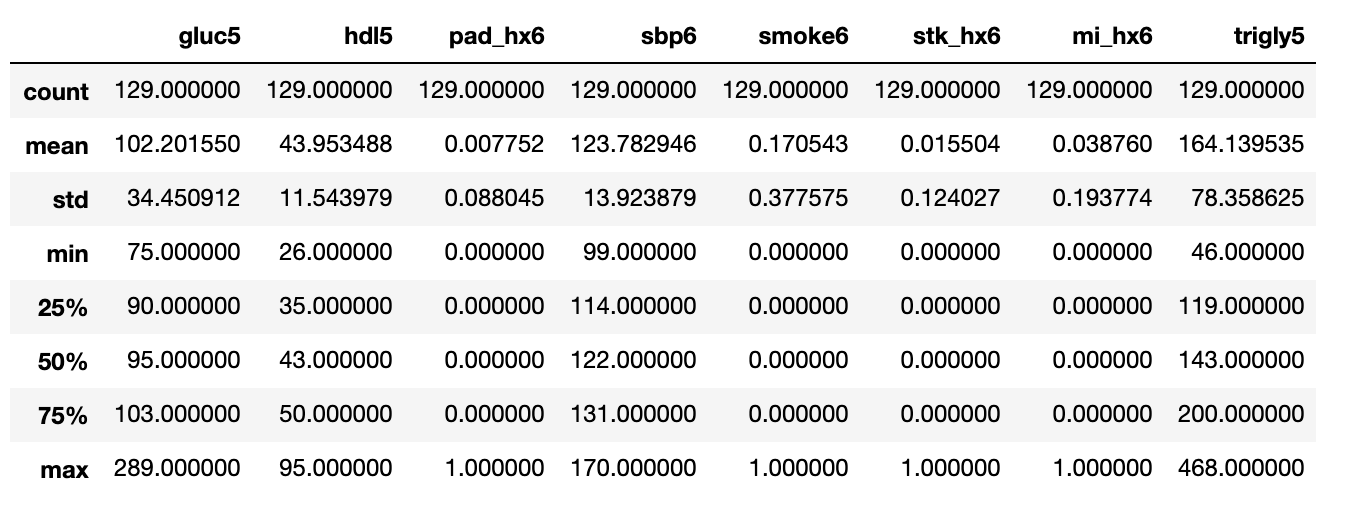
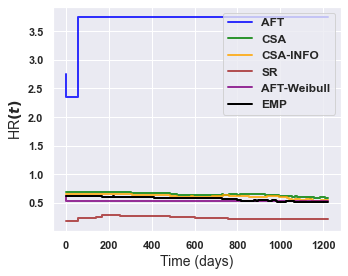
Figure 2(a) demonstrates that CSA-INFO matches the ground truth population hazard, ${\rm HR}(t)$, better than alternative methods on actg-Synthetic data. See the SM for actg and framingham. Figure 2(b) shows sub-population log hazard ratios for four patient clusters obtained via hierarchical clustering on the individual log hazard ratios, $\log{\rm HR}(t|x)$, of the test set of Framingham data. Interestingly, these clusters stratify treatment effects into: positive (2), negative (1 and 3), and neutral (4) sub-populations. Moreover, the estimated density of median $\log{\rm HR}(t|x)$ values in Figure 2(c) illustrates that nearly $70\%$ of the testing set individuals have $\log{\rm HR}(t|x)<0$, thus may benefit from taking statins. Further, we isolated the extreme top and bottom quantiles, ${\rm HR}(t|x)<0.024$ and ${\rm HR}(t|x)>1.916$, respectively, of the median $\log{\rm HR}(t|x)$ values for the test set of Framingham, as shown in Figure 2(c). After comparing their covariates, we found that individuals with the following characteristics may benefit from taking statins: young, male, diabetic, without prior history (CAD, PAD, stroke or MI), high BMI, cholesterol, triglycerides, fasting glucose, and low high-density lipoprotein. Note that individuals with contrasting covariates experience may not benefit from taking statins. There seem to be consensus that diabetics and high-cholesterol patients benefit from statins (Cheung et al., 2004; Wilt et al., 2004). See SM for additional results.

6. Conclusions

We have proposed a unified counterfactual inference framework for survival analysis. Our approach adjusts for bias from two sources, namely, confounding (covariates influence both the treatment assignment and the outcome) and censoring (informative or non-informative). Relative to competitive alternatives, we demonstrate superior performance for both survival-outcome prediction and treatment-effect estimation, across three diverse datasets, including a semi-synthetic dataset which we introduce. Moreover, we formulate a model-free nonparametric hazard ratio metric for comparing treatment effects or leveraging prior randomized real-world experiments in longitudinal studies. We demonstrate that the proposed model-free hazard-ratio estimator can be used to identify or stratify heterogeneous treatment effects. Finally, this work will serve as an important baseline for future work in real-world counterfactual survival analysis. In future work, we plan to understand the sensitivity of our estimates to unobserved confounding (Cornfield et al., 1959) and the effect of both censoring bias and selection bias on causal identifiability.

Supplementary Material for “Enabling Counterfactual Survival Analysis with Balanced Representations"

Anonymous Authors

Appendix A General log-likelihood

The general likelihood-based loss hypothesis that accounts for informative censoring is formulated as:

(13) $$-\ell_{h,\Phi,\nu}(t_{a},c_{a},y,\delta) =\log p_{h,\Phi,\nu}(T_{A},C_{A}|X=x)$$

(14) $$=\log p_{h,\Phi}(T_{A}|X=x)+\log p_{\nu,\Phi}(C_{A}|X=x)\,,$$

where (14) follows from the conditional independence (informative censoring) assumption $T\mathrel{\text{\scalebox{1.07}{$\perp\mkern-10.0mu\perp$}}}C|X,A$. For some parametric formulations of event $p_{h,\Phi}(T_{A}|X=x)$ and censoring $p_{\nu,\Phi}(C_{A}|X=x)$ time distributions, e.g., exponential, Weibull, log-Normal, etc., then $-\ell_{h,\Phi,\nu}(t_{a},c_{a},y,\delta)$ is the closed-form log-likelihood, where:

(15) $$\log p_{h,\Phi}(T_{A}|X=x) \triangleq\delta\cdot\log f_{h,\Phi}(t_{a}|x)+(1-\delta)\cdot\log S_{h,\Phi}(t_{a}|x),$$

(16) $$\log p_{\nu,\Phi}(C_{A}|X=x) \triangleq(1-\delta)\cdot\log e_{\nu,\Phi}(c_{a}|x)+\delta\cdot\log G_{\nu,\Phi}(c_{a}|x),$$

where $\{S_{h,\Phi}(\cdot),G_{\nu,\Phi}(\cdot)\}$ and $\{f_{h,\Phi}(\cdot),e_{\nu,\Phi}(\cdot)\}$ are survival and density functions respectively.

Appendix B Metrics

B.1. Estimands of Interest

Several common estimands of interest include (Zhao et al., 2012; Trinquart et al., 2016):

• Difference in expected lifetime:
  $\textup{ITE}(x)=\int_{0}^{t_{\max}}\{S_{1}(t|x)-S_{0}(t|x)\}\textup{d}t=\mathbb{E}\{T_{1}-T_{0}|X=x\}$.

• Difference in survival function: $\textup{ITE}(t,x)=S_{1}(t|x)-S_{0}(t|x)$.

• Hazard ratio: $\textup{ITE}(t,x)=\lambda_{1}(t|x)/\lambda_{0}(t|x)$.

In our experiments, we consider both the hazard ratio and difference in expected lifetime. The difference of expected lifetime is expressed in terms of both survival functions and expectations:

$$\mathbb{E}[T|X=x] =\int_{-\infty}^{\infty}tf(t|x)dt$$

(17) $$=\int_{0}^{\infty}\left(1-F(t|x)\right)dt-\int_{-\infty}^{0}F(t|x)dt$$

(18) $$=\int_{0}^{t_{\max}}S(t|x)dt\,,$$

where (17) follows from standard properties of expectations and (18) from $1-F(t|x)=S(t|x)$ and $\int_{-\infty}^{0}F(t|x)dt=0$. Below we formulate an approach for estimating the individualized and population hazard ratio.

B.2. Nonparametric Hazard Ratio

To estimate the proposed nonparametric hazard ratio ${\rm HR}(t)$ in (1) we leveraged (1) and $S^{\prime}(t)\triangleq dS(t)/dt$. For the estimator ${\rm\hat{HR}}(t)$, provided that $S(t)$ is a monotonically decreasing function, for simplicity, we fit a linear function $S(t)=m\cdot t+c$ and set $S^{\prime}(t)\approx m$. Further, we leverage $\hat{S}^{\rm PKM}(t)$ in (Chapfuwa et al., 2020), defined as the model-free population point-estimate-based nonparametric Kaplan-Meier (Kaplan and Meier, 1958) estimator. We denote $J$ distinct and ordered observed event times (censored and non-censored) by the set $\mathcal{T}=\{t_{j}|t_{j}>t_{j-1}>\ldots>t_{0}\}$ from $N$ realizations of $Y$. Formally, the population survival $\hat{S}^{\rm PKM}_{A}(t)$ is recursively formulated as

(19) $$\hat{S}^{\rm PKM}_{A}(t_{j}) =\left(1-\frac{\sum_{n:\delta_{n}=1}\mathbb{I}\left(t_{j-1}\leq\gamma(T_{A}^{(n)})<t_{j}\right)}{N-\sum_{n=1}^{N}\mathbb{I}\left(\gamma(T_{A}^{(n)})<t_{j-1}\right)}\right)\hat{S}^{\rm PKM}_{A}(t_{j-1})\,,$$

where $\hat{S}_{A}^{\rm PKM}(t_{0})=1$, and $\mathbb{I}(b)$ represent an indicator function such that $\mathbb{I}(b)=1$ if $b$ holds or $\mathbb{I}(b)=0$ otherwise. Further, $\gamma(\cdot)$ is a deterministic transformation for summarizing $T_{A}$, in our experiments, $\gamma(\cdot)={\rm median(\cdot)}$, computed over samples from $t_{a}\sim p_{h,\Phi}(T_{A}|X=x)$. Note from (19), we marginalize both factual and counterfactual predictions given covariates $x$.

Table 4. Performance comparisons on actg data, with 95% ${\rm HR}(t)$ confidence interval. Test set NN assignment of $y_{\rm{CF}}$ and $\delta_{\rm{CF}}$ yields unbiased ground truth estimator ${\rm HR}(t)=0.54_{(0.51,0.61)}$, since study is a RCT.

Method Causal metric Factual metrics ${\rm HR}(t)$ C-Index (A=0, A=1) Mean COV C-Slope (A=0, A=1) CoxPH-Uniform $0.49_{(0.38,0.64)}$ NA NA NA CoxPH-IPW $0.49_{(0.36,0.68)}$ NA NA NA CoxPH-OW $0.49_{(0.36,0.68)}$ NA NA NA Surv-BART $3.93_{(3.93,4.90)}$ (0.665, 0.845) 0.001 (0.394, 0.517) AFT-Weibull $\textbf{0.53}_{(0.53,0.53)}$ (0.53,0.351) 3.088 (0.847,0.813) AFT-log-Normal $3.75_{(3.75,3.75)}$ (0.717, 0.619) 7.995 (0.847, 0.321) SR $0.21_{(0.21,0.28)}$ (0.628, 0.499) 0 (1.388, 0.442) CSA (proposed) $0.63_{(0.59,0.68)}$ (0.831, 0.814) 0.132 ( 1.042, 1.129) CSA-INFO (proposed) $0.6_{(0.54,0.66)}$ (0.786, 0.822) 0.13 (0.875, 0.938)

A similar formulation for the conditional, individualized ${\rm HR}(t|x)$, can also be derived, where the cumulative density $F_{A}(t|x)=1-S_{A}(t|x)$, is estimated with a Gaussian Kernel Density Estimator (KDE) (Silverman, 1986) on samples from the model, $t_{a}\sim p_{h,\Phi}(T_{A}|X=x)$. Then we have:

Definition 0.

Nonparametric conditional Hazard Ratio and its approximation, ${\rm\hat{HR}}(t|x)$, as where, $S^{\prime}(t|x)\triangleq dS(|t|x)/dt$ is also approximated with fitting a linear function $S(t|x)=m\cdot t+c$, and setting $S^{\prime}(t|x)\approx m$. Note that for some parametric formulations, ${\rm HR}(t|x)$, can be readily evaluated because $f(t_{a}|x)$ and $S(t_{a}|x)$ are available in closed form.

B.3. Factual Metrics

Concordance Index

C-Index (also related to receiver operating characteristic) is a widely used survival ranking metric which naturally handles censoring. It quantifies the consistency between the order of the predicted times or risk scores relative to ground truth. C-Index is evaluated on point estimates, we summarize individualized predicted samples from CSA and CSA-INFO, i.e., $\hat{t}_{a}={\rm median}\left(\{{t_{s}}\}^{200}_{s=1}\right)$, where $t_{s}$ is a sample from the trained model.

Calibration Slope

Calibration quantifies distributional statistical consistency between model predictions relative to ground truth. We measure population calibration by comparing population survival curves from model predictions against ground truth according to (Chapfuwa et al., 2020). We desire a high calibrated model, with calibration slope of 1, while a slope $<1$ and slope $>1$ indicates underestimation or overestimation risk, respectively.

Coefficient of Variation

The coefficient of variation (COV) $\sigma\mu^{-1}$, the ratio between standard deviation and mean, quantifies distribution dispersion. A COV $>1$ and $<1$ indicates a high or low variance distribution, in practice, we desire low variance distribution. We use Mean COV $N^{-1}\sum_{i=1}^{N}\sigma_{i}\mu_{i}^{-1}$, where for subject $i$ we compute $\{\mu_{i},\sigma_{i}\}$ from samples $\{{t_{s}}\}^{200}_{s=1}$.

Appendix C Baselines

Cox proportional hazard (CoxPH)

CoxPH assumes a semi-parametric linear model $\lambda(t|a)=\lambda_{\rm b}(t)\exp(a\beta)$ , thus the hazard ratio between treatment and control can be obtained without specifying the baseline hazard $\lambda_{\rm b}(t)$ as in (12). A simple logistic model $\hat{e}_{i}=\sigma(x_{i};\eta)$, is used to approximate the unknown propensity score $P(A=1|X=x)$. Methods that adjust for selection bias (or confounding) learn $\beta$ by maximizing a propensity weighted partial likelihood (Schemper et al., 2009; Buchanan et al., 2014; Rosenbaum and Rubin, 1983)

(20) $$\mathcal{L}(\beta) =\prod_{i:\delta_{i}=1}\left(\frac{\exp(a_{i}\beta)}{\sum_{j:t_{j}\geq t_{i}}\hat{w}_{j}\cdot\exp(a_{j}\beta)}\right)^{\hat{w_{i}}}\,.$$

We consider three normalized weighting schemes for $w$ , namely, $(i)$ inverse probability weighting (IPW) (Horvitz and Thompson, 1952; Cao et al., 2009), where ${\rm IPW}_{i}=\frac{a_{i}}{\hat{e}_{i}}+\frac{1-a_{i}}{1-\hat{e}_{i}}$, $(ii)$ overlapping weights (OW) (Crump et al., 2006; Li et al., 2018), where ${\rm OW}_{i}=a_{i}\cdot(1-\hat{e}_{i})+(1-a_{i})\cdot\hat{e}_{i}$, and $(iii)$ the standard RCT Uniform assumption. Note that this modeling approach requires fitting over the entire dataset, thus has no inference capability.

Accelerated Failure Time (AFT)

We implement ${\rm IPM}$ regularized neural-based log-Normal and Weibull AFT baselines. Both approaches have a desirable closed form $S_{h,\Phi}(t_{a}|x)$, thus enabling maximum likelihood based estimation, where

$$-\mathcal{L}_{\rm F}^{\rm AFT} \triangleq\mathbb{E}_{(y,\delta,x,a)\sim p(y,\delta,X,A)}\left[\delta\cdot\log f_{h,\Phi}(t_{a}|x)\right.$$

(21) $$+\left.(1-\delta)\cdot\log S_{h,\Phi}(t_{a}|x)\right]\,.$$

The log-Normal mean and variance parameters are learned such that, $\log t_{a}=\mu_{{h,\Phi}}(h(r,a))+\epsilon$, where $\epsilon\sim\mathcal{N}(0,\sigma^{2}_{{h,\Phi}}(h(r,a)))$ and $r=\Phi(x)$. Further, we learn the Weibull scale and shape parameters, where $t_{a}=\lambda_{{h,\Phi}}(h(r,a))\cdot\left(-\log U\right)^{\left(k_{{h,\Phi}}(h(r,a))\right)^{-1}}$ and $U\sim{\rm Uniform}(0,1)$. We regularize (C) with the ${\rm IPM}$ loss, for maximum likelihood optimization.

Semi-supervised regression (SR)

To demonstrate the effectiveness of our flow-based uncertainty estimation approach we contrast CSA with a deterministic accuracy objective from (Chapfuwa et al., 2018), where $t_{a}=h(r,a)$ and:

$$\mathcal{L}_{\rm F}^{\rm SR} \triangleq\mathbb{E}_{(y,\delta,x,a)\sim p(y,\delta,X,A)}\left[\delta\cdot\left(|y-t_{a}|\right)\right.$$

(22) $$+\left.(1-\delta)\cdot\left(\max(0,y-t_{a})\right)\right]\,,$$

where (C) is regularized according to the ${\rm IPM}$ loss.

(a) Framingham ${\rm HR}(t|x)<0.024$

(b) Framingham ${\rm HR}(t|x)>1.916$

Figure 3. Covariate statistics for top (a) and bottom (b) quantiles, of the median $\log{\rm HR}(t|x)$ values for the test set of Framingham.

(a) actg ${\rm HR}(t)$

(b) Framingham ${\rm HR}(t)$

Figure 4. Inferred population ${\rm HR}(t)$ comparisons on (a) actg and (b) framingham datasets.

Survival Bayesian additive regression trees (Surv-BART)

Surv-BART (Sparapani et al., 2016) is a nonparametric tree-based approach for estimating individualized survivals $\hat{S}(t_{a}^{(j)}|X=x)$ (defined at pre-specified $J$ time-horizons) from an ensemble of regression trees. Note, Surv-BART does not adjust for both selection bias and informative censoring. While, we fit two separate models based on factual treatment and control data, causal metrics are estimated with both factual and counterfactual predictions.

Appendix D Experiments

D.1. Generating ATCG-Synthetic Dataset

The actg-Synthetic, is a semi-synthetic dataset based on actg covariates (Hammer et al., 1996). We simulate potential outcomes according to a Gompertz-Cox distribution (Bender et al., 2005) with selection bias from a simple logistic model for $P(A=1|X=x)$ and AFT-based censoring mechanism. Below is our generative scheme:

$$X =\text{ {\sc ACTG} covariates}$$

$$P(A=1|X=x) =\frac{1}{b}\times\left(a+\sigma\left(\eta({\rm AGE}-\mu_{\rm AGE}+{\rm CD40}-\mu_{\rm CD40})\right)\right)$$

$$T_{A} =\frac{1}{\alpha_{A}}\log\left[1-\frac{\alpha_{A}\log U}{\lambda_{A}\exp\left(x^{T}\beta_{A}\right)}\right]$$

$$U \sim{\rm Uniform}(0,1)$$

$$\log C \sim{\rm Normal}(\mu_{c},\sigma_{c}^{2})$$

$$Y =\min(T_{A},C)\,,\quad\delta=1\text{ if }T_{A}<C,\text{ else }\delta=0\,,$$

where $\{\beta_{A},\alpha_{A},\lambda_{A},b,a,\eta,\mu_{c},\sigma_{c}\}$ are hyper-parameters and $\{\mu_{\rm AGE},\mu_{\rm CD40}\}$ are the means for age and CD40 respectively. This semi-synthetic dataset will made publicly available.

D.2. Quantitative Results

See Table 4 for additional quantitative comparisons on actg dataset.

D.3. Qualitative Results

Figure 4 demonstrates model comparisons across of population hazard, ${\rm HR}(t)$, on actg and Framingham datasets. Figure 3, summarizes the positive and negative covariate statistics from the isolated extreme top and bottom quantiles on Framingham datasets.

D.4. Architecture of the neural network

We detail the architecture of neural-based methods, namely, baselines (AFT-log-Normal, AFT-Weibull, SR) and our proposed methods (CSA and CSA-INFO). All methods are trained using one NVIDIA P100 GPU with 16GB memory. In all experiments we set the minibatch size $M=200$, Adam optimizer with the following hyperparameters: learning rate $3\times 10^{-4}$, first moment $0.9$, second moment $0.99$, and epsilon $1\times 10^{-8}$. Further, all network weights are initialed according to ${\rm Uniform}(-0.01,0.01)$. Datasets are split into training, validation and test sets according to 70%, 15% and 15% partitions, respectively, stratified by event and treatment proportions. The validation set is used for hyperparameter search and early stopping. All hidden units in $\{h_{A}(\cdot),\nu_{A}(\cdot)\}$, are characterized by Leaky Rectified Linear Unit (ReLU) activation functions, batch normalization and dropout probability of $p=0.2$ on all layers. The output layers of predicted times $\{T_{A},C_{A}\}$ have an additional exponential transformation.

Encoder

The encoding function $\Phi(\cdot)$ for mapping $r=\Phi(x)$ is shared among all the neural based methods (proposed and baselines) and specified in terms of two-layer MLPs of $100$ hidden units.

Decoder

(a) AFT-log-Normal

(b) AFT-Weibull

(c) SR

Figure 5. Decoding architecture of baselines.

(a) CSA

(b) CSA-INFO

Figure 6. Decoding architecture of proposed methods.

Figure 5 shows the architectural details of the baselines, where the decoding function $h_{A}(\cdot)$ is specified in terms of two-layer MLPs of $100$ hidden units. Further, the proposed planar flow based methods shown in Figure 6, are comprised of two-layer MLPS for $\{h_{A}(\cdot),\nu_{A}(\cdot)\}$ of dimensions $[100,200]$. Moreover, the hidden layers $\{h_{A}^{(2)},\nu_{A}^{(2)}\}$, take as input the concatenated $[h_{A}^{(1)},\tilde{\epsilon}_{h}]$ and $[\nu_{A}^{(1)},\tilde{\epsilon}_{\nu}]$ respectively. Finally, we set the planar flow dimensions for both $\{\tilde{\epsilon}_{\nu},\tilde{\epsilon}_{h}\}$ to $100$.

References

- (1)
- Austin (2007) Peter C Austin. 2007. Propensity-score matching in the cardiovascular surgery literature from 2004 to 2006: a systematic review and suggestions for improvement. The Journal of Thoracic and Cardiovascular Surgery (2007).
- Austin (2014) Peter C Austin. 2014. The use of propensity score methods with survival or time-to-event outcomes: reporting measures of effect similar to those used in randomized experiments. Statistics in Medicine (2014).
- Avati et al. (2020) Anand Avati, Tony Duan, Sharon Zhou, Kenneth Jung, Nigam H Shah, and Andrew Y Ng. 2020. Countdown regression: sharp and calibrated survival predictions. In Uncertainty in Artificial Intelligence.
- Bareinboim and Pearl (2012) Elias Bareinboim and Judea Pearl. 2012. Controlling selection bias in causal inference. In AISTATS.
- Bender et al. (2005) Ralf Bender, Thomas Augustin, and Maria Blettner. 2005. Generating survival times to simulate Cox proportional hazards models. Statistics in medicine (2005).
- Benjamin et al. (1994) Emelia J Benjamin, Daniel Levy, Sonya M Vaziri, Ralph B D’Agostino, Albert J Belanger, and Philip A Wolf. 1994. Independent risk factors for atrial fibrillation in a population-based cohort: the Framingham Heart Study. Jama (1994).
- Buchanan et al. (2014) Ashley L Buchanan, Michael G Hudgens, Stephen R Cole, Bryan Lau, Adaora A Adimora, and Women’s Interagency HIV Study. 2014. Worth the weight: using inverse probability weighted Cox models in AIDS research. AIDS research and human retroviruses (2014).
- Cao et al. (2009) Weihua Cao, Anastasios A Tsiatis, and Marie Davidian. 2009. Improving efficiency and robustness of the doubly robust estimator for a population mean with incomplete data. Biometrika (2009).
- Chapfuwa et al. (2020) P. Chapfuwa, C. Tao, C. Li, I. Khan, K. J. Chandross, M. J. Pencina, L. Carin, and R. Henao. 2020. Calibration and Uncertainty in Neural Time-to-Event Modeling. IEEE Transactions on Neural Networks and Learning Systems (2020).
- Chapfuwa et al. (2018) Paidamoyo Chapfuwa, Chenyang Tao, Chunyuan Li, Courtney Page, Benjamin Goldstein, Lawrence Carin, and Ricardo Henao. 2018. Adversarial time-to-event modeling. In ICML.
- Cheung et al. (2004) Bernard MY Cheung, Ian J Lauder, Chu-Pak Lau, and Cyrus R Kumana. 2004. Meta-analysis of large randomized controlled trials to evaluate the impact of statins on cardiovascular outcomes. British journal of clinical pharmacology (2004).
- Chipman et al. (2010) Hugh A Chipman, Edward I George, Robert E McCulloch, et al. 2010. BART: Bayesian additive regression trees. The Annals of Applied Statistics (2010).
- Cole and Hernán (2004) Stephen R Cole and Miguel A Hernán. 2004. Adjusted survival curves with inverse probability weights. Computer methods and programs in biomedicine (2004).
- Cornfield et al. (1959) Jerome Cornfield, William Haenszel, E Cuyler Hammond, Abraham M Lilienfeld, Michael B Shimkin, and Ernst L Wynder. 1959. Smoking and lung cancer: recent evidence and a discussion of some questions. Journal of the National Cancer institute (1959).
- Cox (1972) David R Cox. 1972. Regression models and life-tables. Journal of the Royal Statistical Society: Series B (Methodological) (1972).
- Crump et al. (2006) Richard K Crump, V Joseph Hotz, Guido W Imbens, and Oscar A Mitnik. 2006. Moving the goalposts: Addressing limited overlap in the estimation of average treatment effects by changing the estimand. Technical Report. National Bureau of Economic Research.
- Cui et al. (2020) Yifan Cui, Michael R Kosorok, Stefan Wager, and Ruoqing Zhu. 2020. Estimating heterogeneous treatment effects with right-censored data via causal survival forests. arXiv (2020).
- Cuturi (2013) Marco Cuturi. 2013. Sinkhorn distances: Lightspeed computation of optimal transport. In NeurIPS.
- Díaz (2019) Iván Díaz. 2019. Statistical inference for data-adaptive doubly robust estimators with survival outcomes. Statistics in Medicine (2019).
- Frankovich et al. (2011) Jennifer Frankovich, Christopher A Longhurst, and Scott M Sutherland. 2011. Evidence-based medicine in the EMR era. N Engl J Med (2011).
- Gombar et al. (2019) Saurabh Gombar, Alison Callahan, Robert Califf, Robert Harrington, and Nigam H Shah. 2019. It is time to learn from patients like mine. NPJ digital medicine (2019).
- Hammer et al. (1996) Scott M Hammer, David A Katzenstein, Michael D Hughes, Holly Gundacker, Robert T Schooley, Richard H Haubrich, W Keith Henry, Michael M Lederman, John P Phair, Manette Niu, et al. 1996. A trial comparing nucleoside monotherapy with combination therapy in HIV-infected adults with CD4 cell counts from 200 to 500 per cubic millimeter. New England Journal of Medicine (1996).
- Harrell Jr et al. (1984) Frank E Harrell Jr, Kerry L Lee, Robert M Califf, David B Pryor, and Robert A Rosati. 1984. Regression modelling strategies for improved prognostic prediction. Statistics in medicine (1984).
- Häyrinen et al. (2008) Kristiina Häyrinen, Kaija Saranto, and Pirkko Nykänen. 2008. Definition, structure, content, use and impacts of electronic health records: a review of the research literature. International Journal of Medical Informatics (2008).
- Henderson et al. (2020) Nicholas C Henderson, Thomas A Louis, Gary L Rosner, and Ravi Varadhan. 2020. Individualized treatment effects with censored data via fully nonparametric Bayesian accelerated failure time models. Biostatistics (2020).
- Hernán et al. (2000) Miguel Ángel Hernán, Babette Brumback, and James M Robins. 2000. Marginal structural models to estimate the causal effect of zidovudine on the survival of HIV-positive men. Epidemiology (2000).
- Hernán et al. (2005) Miguel A Hernán, Stephen R Cole, Joseph Margolick, Mardge Cohen, and James M Robins. 2005. Structural accelerated failure time models for survival analysis in studies with time-varying treatments. Pharmacoepidemiology and Drug Safety (2005).
- Hernán and Robins (2020) Miguel A Hernán and James M Robins. 2020. Causal inference: what if. Boca Raton: Chapman & Hill/CRC (2020).
- Hill (2011) Jennifer L Hill. 2011. Bayesian nonparametric modeling for causal inference. Journal of Computational and Graphical Statistics (2011).
- Horvitz and Thompson (1952) Daniel G Horvitz and Donovan J Thompson. 1952. A generalization of sampling without replacement from a finite universe. Journal of the American statistical Association (1952).
- Hu et al. (2020) Liangyuan Hu, Jiayi Ji, and Fan Li. 2020. Estimating heterogeneous survival treatment effect in observational data using machine learning. arXiv (2020).
- Ishwaran et al. (2008) Hemant Ishwaran, Udaya B Kogalur, Eugene H Blackstone, Michael S Lauer, et al. 2008. Random survival forests. The annals of applied statistics (2008).
- Jha et al. (2009) Ashish K Jha, Catherine M DesRoches, Eric G Campbell, Karen Donelan, Sowmya R Rao, Timothy G Ferris, Alexandra Shields, Sara Rosenbaum, and David Blumenthal. 2009. Use of electronic health records in US hospitals. New England Journal of Medicine (2009).
- Kaplan and Meier (1958) Edward L Kaplan and Paul Meier. 1958. Nonparametric estimation from incomplete observations. Journal of the American statistical association (1958).
- Katzman et al. (2018) Jared L Katzman, Uri Shaham, Alexander Cloninger, Jonathan Bates, Tingting Jiang, and Yuval Kluger. 2018. DeepSurv: personalized treatment recommender system using a Cox proportional hazards deep neural network. BMC medical research methodology (2018).
- Kleinbaum and Klein (2010) David G Kleinbaum and Mitchel Klein. 2010. Survival analysis. Springer.
- Lee et al. (2019) Changhee Lee, William R Zame, Ahmed M Alaa, and Mihaela van der Schaar. 2019. Temporal Quilting for Survival Analysis. In AISTATS.
- Lee et al. (2018) Changhee Lee, William R Zame, Jinsung Yoon, and Mihaela van der Schaar. 2018. Deephit: A deep learning approach to survival analysis with competing risks. In AAAI.
- Li et al. (2018) Fan Li, Kari Lock Morgan, and Alan M Zaslavsky. 2018. Balancing covariates via propensity score weighting. J. Amer. Statist. Assoc. (2018).
- Longhurst et al. (2014) Christopher A Longhurst, Robert A Harrington, and Nigam H Shah. 2014. A ‘green button’for using aggregate patient data at the point of care. Health affairs (2014).
- Mihaylova et al. (2012) B Mihaylova, J Emberson, L Blackwell, A Keech, J Simes, EH Barnes, M Voysey, 3A Gray, R Collins, and C Baigent. 2012. The effects of lowering LDL cholesterol with statin therapy in people at low risk of vascular disease: meta-analysis of individual data from 27 randomised trials.
- Miscouridou et al. (2018) Xenia Miscouridou, Adler Perotte, Noémie Elhadad, and Rajesh Ranganath. 2018. Deep survival analysis: Nonparametrics and missingness. In Machine Learning for Healthcare Conference.
- Müller (1997) Alfred Müller. 1997. Integral probability metrics and their generating classes of functions. Advances in Applied Probability (1997).
- Nagpal et al. (2021) Chirag Nagpal, Xinyu Rachel Li, and Artur Dubrawski. 2021. Deep survival machines: Fully parametric survival regression and representation learning for censored data with competing risks. IEEE Journal of Biomedical and Health Informatics (2021).
- Ranganath et al. (2016) Rajesh Ranganath, Adler Perotte, Noémie Elhadad, and David Blei. 2016. Deep survival analysis. In Machine Learning for Healthcare Conference.
- Rezende and Mohamed (2015) Danilo Jimenez Rezende and Shakir Mohamed. 2015. Variational inference with normalizing flows. In ICML.
- Robins (1986) James Robins. 1986. A new approach to causal inference in mortality studies with a sustained exposure period—application to control of the healthy worker survivor effect. Mathematical modelling (1986).
- Rosenbaum and Rubin (1983) Paul R Rosenbaum and Donald B Rubin. 1983. The central role of the propensity score in observational studies for causal effects. Biometrika (1983).
- Rubin (2005) Donald B Rubin. 2005. Causal Inference Using Potential Outcomes. J. Amer. Statist. Assoc. (2005).
- Schemper et al. (2009) Michael Schemper, Samo Wakounig, and Georg Heinze. 2009. The estimation of average hazard ratios by weighted Cox regression. Statistics in medicine (2009).
- Shalit et al. (2017) Uri Shalit, Fredrik D Johansson, and David Sontag. 2017. Estimating individual treatment effect: generalization bounds and algorithms. In ICML.
- Shen et al. (2018) Jincheng Shen, Lu Wang, Stephanie Daignault, Daniel E Spratt, Todd M Morgan, and Jeremy MG Taylor. 2018. Estimating the optimal personalized treatment strategy based on selected variables to prolong survival via random survival forest with weighted bootstrap. Journal of biopharmaceutical statistics (2018).
- Silverman (1986) Bernard W Silverman. 1986. Density estimation for statistics and data analysis. CRC press.
- Sparapani et al. (2016) Rodney A Sparapani, Brent R Logan, Robert E McCulloch, and Purushottam W Laud. 2016. Nonparametric survival analysis using Bayesian additive regression trees (BART). Statistics in medicine (2016).
- Sriperumbudur et al. (2012) Bharath K Sriperumbudur, Kenji Fukumizu, Arthur Gretton, Bernhard Schölkopf, Gert RG Lanckriet, et al. 2012. On the empirical estimation of integral probability metrics. Electronic Journal of Statistics (2012).
- Trinquart et al. (2016) Ludovic Trinquart, Justine Jacot, Sarah C Conner, and Raphaël Porcher. 2016. Comparison of treatment effects measured by the hazard ratio and by the ratio of restricted mean survival times in oncology randomized controlled trials. Journal of Clinical Oncology (2016).
- Tsiatis (2007) Anastasios Tsiatis. 2007. Semiparametric theory and missing data. Springer Science & Business Media.
- van der Laan and Robins (2003) Mark J van der Laan and James M Robins. 2003. Unified Approach for Causal Inference and Censored Data. In Unified Methods for Censored Longitudinal Data and Causality. Springer.
- Van der Laan and Rose (2011) Mark J Van der Laan and Sherri Rose. 2011. Targeted learning: causal inference for observational and experimental data. Springer Science & Business Media.
- Villani (2008) Cédric Villani. 2008. Optimal transport: old and new. Springer Science & Business Media.
- Wager and Athey (2018) Stefan Wager and Susan Athey. 2018. Estimation and inference of heterogeneous treatment effects using random forests. J. Amer. Statist. Assoc. (2018).
- Wei (1992) Lee-Jen Wei. 1992. The accelerated failure time model: a useful alternative to the Cox regression model in survival analysis. Statistics in medicine (1992).
- Wilt et al. (2004) Timothy J Wilt, Hanna E Bloomfield, Roderick MacDonald, David Nelson, Indulis Rutks, Michael Ho, Gregory Larsen, Anthony McCall, Sandra Pineros, and Anne Sales. 2004. Effectiveness of statin therapy in adults with coronary heart disease. Archives of internal medicine (2004).
- Xiu et al. (2020) Zidi Xiu, Chenyang Tao, and Ricardo Henao. 2020. Variational learning of individual survival distributions. In Proceedings of the ACM Conference on Health, Inference, and Learning.
- Yusuf et al. (2016) Salim Yusuf, Jackie Bosch, Gilles Dagenais, Jun Zhu, Denis Xavier, Lisheng Liu, Prem Pais, Patricio López-Jaramillo, Lawrence A Leiter, Antonio Dans, et al. 2016. Cholesterol lowering in intermediate-risk persons without cardiovascular disease. New England Journal of Medicine (2016).
- Zhang et al. (2020) Yao Zhang, Alexis Bellot, and Mihaela van der Schaar. 2020. Learning Overlapping Representations for the Estimation of Individualized Treatment Effects. In AISTATS.
- Zhao et al. (2012) Lihui Zhao, Lu Tian, Hajime Uno, Scott D Solomon, Marc A Pfeffer, Jerald S Schindler, and Lee Jen Wei. 2012. Utilizing the integrated difference of two survival functions to quantify the treatment contrast for designing, monitoring, and analyzing a comparative clinical study. Clinical trials (2012).