Optimal Rates for Estimation of Two-Dimensional Totally Positive Distributions

Jan-Christian Hütterlabel=e1]jhuetter@broadinstitute.org [    Cheng Maolabel=e2]cheng.mao@math.gatech.edu [    Philippe Rigolletlabel=e3]rigollet@math.mit.edu [    Elina Robevalabel=e4]erobeva@math.ubc.ca [ Broad Institute, 415 Main Street, Cambridge, MA, 02142, USA. School of Mathematics, Georgia Institute of Technology, Suite 117, 686 Cherry Street, Atlanta, GA, 30332-0160, USA. Department of Mathematics, Massachusetts Institute of Technology, Building 2, Room 106, 77 Massachusetts Avenue, Cambridge, MA, 02139-4307, USA. Department of Mathematics, University of British Columbia, Room 121, 1984 Mathematics Road, Vancouver, BC, V6T 1Z2, Canada.
(0000)
Abstract

We study minimax estimation of two-dimensional totally positive distributions. Such distributions pertain to pairs of strongly positively dependent random variables and appear frequently in statistics and probability. In particular, for distributions with β𝛽\beta-Hölder smooth densities where β(0,2)𝛽02\beta\in(0,2), we observe polynomially faster minimax rates of estimation when, additionally, the total positivity condition is imposed. Moreover, we demonstrate fast algorithms to compute the proposed estimators and corroborate the theoretical rates of estimation by simulation studies.

62G05, 62G07,
totally positive distributions,
nonparametric density estimation,
shape-constrained estimation,
doi:
10.1214/154957804100000000
keywords:
[class=MSC]
keywords:
volume: 0

, , and

1 Introduction

For a set 𝒳=i=1d𝒳i𝒳superscriptsubscriptproduct𝑖1𝑑subscript𝒳𝑖\mathcal{X}=\prod_{i=1}^{d}\mathcal{X}_{i} where each 𝒳isubscript𝒳𝑖\mathcal{X}_{i} is totally ordered111A set 𝒳𝒳\mathcal{X} is totally ordered if it is equipped with a total order, that is, a binary relation which is antisymmetric, transitive and connex. This work is only concerned with 𝒳𝒳\mathcal{X}\subseteq\mathbbm{R} equipped with its natural order., a function p:𝒳:𝑝𝒳p:\mathcal{X}\to\mathbbm{R} is called multivariate totally positive of order 2 (MTP2subscriptMTP2\mathrm{MTP}_{2}[22, 24] if

p(xy)p(xy)p(x)p(y),x,y𝒳,formulae-sequence𝑝𝑥𝑦𝑝𝑥𝑦𝑝𝑥𝑝𝑦for-all𝑥𝑦𝒳\displaystyle p(x\wedge y)p(x\vee y)\geq p(x)p(y)\,,\qquad\forall\,x,y\in\mathcal{X}, (1.1)

where \land and \lor denote the coordinate-wise min and max operators respectively. The MTP2subscriptMTP2\mathrm{MTP}_{2} condition is also known as the FKG lattice condition because of its central role in the FKG inequality [14]. It is sometimes referred to as log-supermodularity because of its similarity up to morphism to supermodularity [18, 37]. Throughout, we say that a probability distribution is MTP2subscriptMTP2\mathrm{MTP}_{2} if it has an MTP2subscriptMTP2\mathrm{MTP}_{2} density.

A variety of joint distributions are known to be MTP2subscriptMTP2\mathrm{MTP}_{2}, for example, order statistics of i.i.d. variables, eigenvalues of Wishart matrices [24], and ferromagnetic Ising models [28]. Furthermore, Gaussian and binary latent tree models are signed MTP2subscriptMTP2\mathrm{MTP}_{2}, that is, there exists a sign change of each coordinate making the distribution MTP2subscriptMTP2\mathrm{MTP}_{2} [25, 27]. In particular, all these distributions exhibit positive association, a marked feature of MTP2subscriptMTP2\mathrm{MTP}_{2} distributions. As opposed to positive association, however, the MTP2subscriptMTP2\mathrm{MTP}_{2} property is preserved after conditioning or marginalization [24]. As a result of their frequent appearances, MTP2subscriptMTP2\mathrm{MTP}_{2} distributions have long been studied in statistics and probability [24, 26, 2, 8, 44, 27, 38].

In this paper, we study minimax estimation of an MTP2subscriptMTP2\mathrm{MTP}_{2} distribution in dimension two222In dimension two, MTP2subscriptMTP2\mathrm{MTP}_{2} is sometimes simply called TP2subscriptTP2\mathrm{TP}_{2} for totally positive of order 2. from i.i.d. observations. We mainly focus on distributions on the square [0,1]2superscript012[0,1]^{2} for which density functions exist. Since almost surely no four observations from such a distribution form a rectangle, the MTP2subscriptMTP2\mathrm{MTP}_{2} constraint (1.1) is inactive on the observations and consequently, the maximum likelihood estimator over this class does not exist (see Lemma 14 and Remark 15 in Appendix A). Therefore, we further assume that the distribution has a β𝛽\beta-Hölder smooth density, a widely adopted assumption in nonparametric estimation [46].

Smooth MTP2subscriptMTP2\mathrm{MTP}_{2} distributions have long been studied in the literature. Examples include, but are not limited to, (1) pairwise marginals of Gaussian latent tree models [13], such as Brownian motion tree models and factor analysis models, (2) joint distributions of pairs of time points of a strong Markov process on the real line with continuous paths [23], such as a diffusion process, and (3) MTP2subscriptMTP2\mathrm{MTP}_{2} transelliptical distributions, such as MTP2subscriptMTP2\mathrm{MTP}_{2} multivariate t𝑡t-distributions, which are commonly used in finance [1].

Main contribution

Our main results can be stated informally as follows.

Theorem 1 (Informal statement of minimax rates).

Given N𝑁N i.i.d. observations from a two-dimensional distribution with an MTP2subscriptMTP2\mathrm{MTP}_{2} and β𝛽\beta-Hölder smooth density, the minimax rate of estimation in the squared Hellinger distance is (up to a polylogarithmic factor)

{N2β2β+1, if  0.5β<1,N2/3, if  1β<2,N2β2β+2, if β2.casessuperscript𝑁2𝛽2𝛽1 if 0.5𝛽1superscript𝑁23 if 1𝛽2superscript𝑁2𝛽2𝛽2 if 𝛽2\begin{cases}N^{-\frac{2\beta}{2\beta+1}},&\text{ if }\ 0.5\leq\beta<1,\\ N^{-2/3},&\text{ if }\ 1\leq\beta<2,\\ N^{-\frac{2\beta}{2\beta+2}},&\text{ if }\ \beta\geq 2.\end{cases} (1.2)

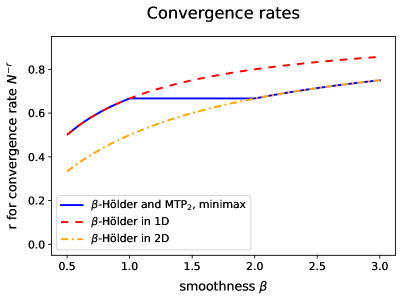
It is well known that without the MTP2subscriptMTP2\mathrm{MTP}_{2} assumption, the minimax rates for the β𝛽\beta-Hölder class in dimension d𝑑d scale as N2β2β+dsuperscript𝑁2𝛽2𝛽𝑑N^{-\frac{2\beta}{2\beta+d}} up to a polylogarithmic factor, under various comparable models and error metrics (see, for example, [33]). Hence, our results show that for 0.5β<10.5𝛽10.5\leq\beta<1, the minimax rate exhibits a one-dimensional behavior thanks to the MTP2subscriptMTP2\mathrm{MTP}_{2} constraint; for 1β<21𝛽21\leq\beta<2, the rate is polynomially faster than that without the MTP2subscriptMTP2\mathrm{MTP}_{2} constraint and is independent of the smoothness parameter β𝛽\beta; for β>2𝛽2\beta>2, however, the MTP2subscriptMTP2\mathrm{MTP}_{2} constraint has no effect on the minimax rate (see Figure 1 for a visualization).

Note that results similar to what we obtain for MTP2subscriptMTP2\mathrm{MTP}_{2} are expected to arise when p𝑝p is assumed to be smooth and log-concave. However, MTP2subscriptMTP2\mathrm{MTP}_{2} only makes assumptions on the behavior of the function along lattice directions. While this is not directly comparable with log-concavity, it is, in essence, a weaker condition in the sense that it imposes a less stringent structure on the density. Our results indicate that when coupled with smoothness, MTP2subscriptMTP2\mathrm{MTP}_{2} makes up for this deficiency and leads to the same rates of convergence.

Our results for the regime 0<β<0.50𝛽0.50<\beta<0.5 are unfortunately inconclusive, but the upper bounds exhibit polynomial improvement in the rates when MTP2subscriptMTP2\mathrm{MTP}_{2} is assumed; see (3.12) below.

Refer to caption
Figure 1: Visual comparison of the estimation rate for β𝛽\beta-Hölder smooth MTP2subscriptMTP2\mathrm{MTP}_{2} distributions in Theorem 1, with estimation rates for β𝛽\beta-Hölder smooth distributions (without the MTP2subscriptMTP2\mathrm{MTP}_{2} constraint) in 1D and 2D, suppressing logarithmic factors.

As a stepping stone to this problem, we also consider the following discrete version of MTP2subscriptMTP2\mathrm{MTP}_{2}. A distribution on the grid [n1]×[n2]delimited-[]subscript𝑛1delimited-[]subscript𝑛2[n_{1}]\times[n_{2}] is MTP2subscriptMTP2\mathrm{MTP}_{2} if its probability mass function (PMF) p𝑝p, which is an n1×n2subscript𝑛1subscript𝑛2n_{1}\times n_{2} matrix, fulfills (1.1). Thus, MTP2subscriptMTP2\mathrm{MTP}_{2} says that all the 2×2222\times 2 minors of p𝑝p are non-negative:

pijpkpipkj,for all 1i<kn1,1j<n2.formulae-sequenceformulae-sequencesubscript𝑝𝑖𝑗subscript𝑝𝑘subscript𝑝𝑖subscript𝑝𝑘𝑗for all 1𝑖𝑘subscript𝑛11𝑗subscript𝑛2\displaystyle p_{ij}p_{k\ell}\geq p_{i\ell}p_{kj},\qquad\text{for all }1\leq i<k\leq n_{1},1\leq j<\ell\leq n_{2}. (1.3)

We study estimation of the PMF p𝑝p from N𝑁N independent observations in this discrete setup.

To obtain upper bounds for estimation of a discrete MTP2subscriptMTP2\mathrm{MTP}_{2} distribution, we employ a variant of the maximum likelihood estimator (MLE) defined in Section 2.1. For estimating a smooth MTP2subscriptMTP2\mathrm{MTP}_{2} density, we first discretize the space [0,1]2superscript012[0,1]^{2} and then apply the discrete MLE to obtain an estimator (defined in Section 3.1) that achieves near-optimal upper bounds. Both estimators are computationally efficient, with the implementations discussed in more detail in Section 4.

Related work. There has been a recent surge of interest in the estimation of MTP2subscriptMTP2\mathrm{MTP}_{2} distributions. The special case of Gaussian MTP2subscriptMTP2\mathrm{MTP}_{2} distributions has been studied by [44, 27] from the perspective of maximum likelihood estimation and optimization. Maximum likelihood estimation of log-concave MTP2subscriptMTP2\mathrm{MTP}_{2} distributions was also analyzed recently [39, 38]. However, no statistical rate of estimation of MTP2subscriptMTP2\mathrm{MTP}_{2} distributions is currently known. The present paper establishes the first minimax rates (up to logarithmic factors) of estimation of a smooth MTP2subscriptMTP2\mathrm{MTP}_{2} density.

More broadly, our work falls into the scope of nonparametric density estimation which is a fundamental problem in nonparametric estimation. As such it has received considerable attention over the years [20, 41, 49, 7, 43]. A central paradigm in this literature is to assume smoothness of the underlying density to be estimated. Such an assumption justifies a variety of statistical methods ranging from kernel density estimation to series expansions. Another approach to nonparametric estimation, and in particular to density estimation, is to use shape constraints whereby the (local) smoothness assumption is dropped and favored by a (global) synthetic constraint such as monotonicity [15, 36], convexity [17, 42] and log-concavity [48, 11, 9, 40] (see [16] for a recent overview). As explained above, the MTP2subscriptMTP2\mathrm{MTP}_{2} constraint alone does not make the density estimation problem well-defined and it has been combined with another shape constraint, namely log-concavity, in [38]. Instead, the present work combines MTP2subscriptMTP2\mathrm{MTP}_{2} with smoothness to obtain a faster statistical rate than with smoothness alone, thus demonstrating compatibility of the local and the global approach.

As we have discussed above, MTP2subscriptMTP2\mathrm{MTP}_{2} is also called log-supermodular. In the recent paper [19], we studied estimation of supermodular matrices (also known as anti-Monge matrices) under sub-Gaussian noise. We note that the proof techniques used in [19] are the starting point for the proofs in this paper, but are extended to the context density estimation. In a parallel work [12], the authors study a related but slightly different model under Gaussian noise, and their proof techniques could potentially be extended to yield rates similar to the ones found in this paper.

Organization. We present the main results of the paper: upper and lower bounds for the discrete case in Section 2, followed by the continuous case in Section 3. All proofs are postponed to Section 6. The implementation of our estimators is discussed in Section 4. Our theoretical results are complemented by numerical experiments on synthetic data in Section 5. Finally, Section 7 includes a conclusion of the paper and a discussion of questions left for future research.

Notation. For a positive integer n𝑛n, let [n]={1,2,,n}delimited-[]𝑛12𝑛[n]=\{1,2,\ldots,n\}. For a finite set S𝑆S, we use |S|𝑆|S| to denote its cardinality. For two sequences {an}n=1superscriptsubscriptsubscript𝑎𝑛𝑛1\{a_{n}\}_{n=1}^{\infty} and {bn}n=1superscriptsubscriptsubscript𝑏𝑛𝑛1\{b_{n}\}_{n=1}^{\infty} of real numbers, we write anbnless-than-or-similar-tosubscript𝑎𝑛subscript𝑏𝑛a_{n}\lesssim b_{n} if there is a universal constant C>0𝐶0C>0 such that anCbnsubscript𝑎𝑛𝐶subscript𝑏𝑛a_{n}\leq Cb_{n} for all n1𝑛1n\geq 1. The relation anbngreater-than-or-equivalent-tosubscript𝑎𝑛subscript𝑏𝑛a_{n}\gtrsim b_{n} is defined analogously. We use c𝑐c and C𝐶C (possibly with subscripts) to denote universal positive constants that may change from line to line. Given a matrix Mn1×n2𝑀superscriptsubscript𝑛1subscript𝑛2M\in\mathbbm{R}^{n_{1}\times n_{2}}, we denote its i𝑖ith row by Mi,subscript𝑀𝑖M_{i,\cdot} and its j𝑗jth column by M,jsubscript𝑀𝑗M_{\cdot,j}. For an entrywise positive vector wn𝑤superscript𝑛w\in\mathbbm{R}^{n} and a vector vn𝑣superscript𝑛v\in\mathbbm{R}^{n}, we use the notation

vw:=(i=1nwivi2)1/2assignsubscriptnorm𝑣𝑤superscriptsuperscriptsubscript𝑖1𝑛subscript𝑤𝑖superscriptsubscript𝑣𝑖212\|v\|_{w}:=\Big{(}\sum_{i=1}^{n}w_{i}v_{i}^{2}\Big{)}^{1/2} (1.4)

for the w𝑤w-weighted 2subscript2\ell_{2} norm of the vector v𝑣v. Similarly, for an entrywise positive matrix bn1×n2𝑏superscriptsubscript𝑛1subscript𝑛2b\in\mathbbm{R}^{n_{1}\times n_{2}} and a matrix an1×n2𝑎superscriptsubscript𝑛1subscript𝑛2a\in\mathbbm{R}^{n_{1}\times n_{2}}, we use absubscriptnorm𝑎𝑏\|a\|_{b} to denote the b𝑏b-weighted Frobenius norm of a𝑎a. For a reference measure μ𝜇\mu on a (continuous or discrete) space 𝒳𝒳\mathcal{X}, and two distributions with probability density or mass functions p𝑝p and q𝑞q respectively, we let

𝗁(p,q):=(𝒳(p(x)q(x))2𝑑μ(x))1/2 and 𝖪𝖫(p,q):=𝒳p(x)logp(x)q(x)dμ(x)formulae-sequenceassign𝗁𝑝𝑞superscriptsubscript𝒳superscript𝑝𝑥𝑞𝑥2differential-d𝜇𝑥12 and assign𝖪𝖫𝑝𝑞subscript𝒳𝑝𝑥𝑝𝑥𝑞𝑥𝑑𝜇𝑥\displaystyle\operatorname{\mathsf{h}}(p,q):=\Big{(}\int_{\mathcal{X}}\big{(}\sqrt{p(x)}-\sqrt{q(x)}\,\big{)}^{2}d\mu(x)\Big{)}^{1/2}\quad\text{ and }\quad\operatorname{\mathsf{KL}}(p,q):=\int_{\mathcal{X}}p(x)\log\frac{p(x)}{q(x)}d\mu(x)

denote the Hellinger distance and the Kullback-Leibler (KL) divergence between the two distributions respectively.

2 𝐌𝐓𝐏𝟐subscript𝐌𝐓𝐏2\mathbf{MTP_{2}} distribution estimation on a grid

Let psuperscript𝑝p^{\ast} be a probability mass function (PMF) on the grid [n1]×[n2]delimited-[]subscript𝑛1delimited-[]subscript𝑛2[n_{1}]\times[n_{2}], where we assume without loss of generality that n1n2subscript𝑛1subscript𝑛2n_{1}\geq n_{2}. In the case where n1n2subscript𝑛1subscript𝑛2n_{1}\leq n_{2}, our results and proofs remain valid with the roles of n1subscript𝑛1n_{1} and n2subscript𝑛2n_{2} swapped. Suppose that psuperscript𝑝p^{*} satisfies the MTP2subscriptMTP2\mathrm{MTP}_{2} condition

pi,jpi+1,j+1pi,j+1pi+1,jfor all i[n11],j[n21].formulae-sequencesubscriptsuperscript𝑝𝑖𝑗subscriptsuperscript𝑝𝑖1𝑗1subscriptsuperscript𝑝𝑖𝑗1subscriptsuperscript𝑝𝑖1𝑗formulae-sequencefor all 𝑖delimited-[]subscript𝑛11𝑗delimited-[]subscript𝑛21\displaystyle p^{\ast}_{i,j}p^{\ast}_{i+1,j+1}\geq p^{\ast}_{i,j+1}p^{\ast}_{i+1,j}\qquad\text{for all }i\in[n_{1}-1],\,j\in[n_{2}-1]. (2.1)

Note that this is equivalent to condition (1.3) by a telescoping sum argument.

Suppose that we are given N𝑁N i.i.d. observations {Zk}k=1Nsuperscriptsubscriptsubscript𝑍𝑘𝑘1𝑁\{Z_{k}\}_{k=1}^{N} from the distribution on [n1]×[n2]delimited-[]subscript𝑛1delimited-[]subscript𝑛2[n_{1}]\times[n_{2}] with PMF psuperscript𝑝p^{*}, that is, each Zk=(i,j)subscript𝑍𝑘𝑖𝑗Z_{k}=(i,j) with probability pi,jsubscriptsuperscript𝑝𝑖𝑗p^{*}_{i,j} for (i,j)[n1]×[n2]𝑖𝑗delimited-[]subscript𝑛1delimited-[]subscript𝑛2(i,j)\in[n_{1}]\times[n_{2}]. Our goal is to estimate psuperscript𝑝p^{\ast}. The number of observations at each point (i,j)𝑖𝑗(i,j) on the grid [n1]×[n2]delimited-[]subscript𝑛1delimited-[]subscript𝑛2[n_{1}]\times[n_{2}] is recorded in a matrix Y=(Yi,j)i[n1],j[n2]𝑌subscriptsubscript𝑌𝑖𝑗formulae-sequence𝑖delimited-[]subscript𝑛1𝑗delimited-[]subscript𝑛2Y=(Y_{i,j})_{i\in[n_{1}],\,j\in[n_{2}]}, defined by

Yi,j:=k=1N𝟙{Zk=(i,j)}.assignsubscript𝑌𝑖𝑗superscriptsubscript𝑘1𝑁1subscript𝑍𝑘𝑖𝑗\displaystyle Y_{i,j}:=\sum_{k=1}^{N}\mathbbm{1}\{Z_{k}=(i,j)\}. (2.2)

Then Y𝑌Y can be viewed as a multinomial random variable with distribution denoted by 𝖬𝗎𝗅𝗍𝗂(N,p)𝖬𝗎𝗅𝗍𝗂𝑁superscript𝑝\mathsf{Multi}(N,p^{*}).

In addition, we define

p𝗆𝗂𝗇:=mini[n1],j[n2]pi,j and p𝗆𝖺𝗑:=maxi[n1],j[n2]pi,j,formulae-sequenceassignsubscriptsuperscript𝑝𝗆𝗂𝗇subscriptformulae-sequence𝑖delimited-[]subscript𝑛1𝑗delimited-[]subscript𝑛2subscriptsuperscript𝑝𝑖𝑗 and assignsubscriptsuperscript𝑝𝗆𝖺𝗑subscriptformulae-sequence𝑖delimited-[]subscript𝑛1𝑗delimited-[]subscript𝑛2subscriptsuperscript𝑝𝑖𝑗p^{\ast}_{\mathsf{min}}:=\min_{i\in[n_{1}],\,j\in[n_{2}]}p^{*}_{i,j}\quad\text{ and }\quad p^{\ast}_{\mathsf{max}}:=\max_{i\in[n_{1}],\,j\in[n_{2}]}p^{*}_{i,j},

and assume a mild lower bound on the sample size N12log(n1n2/δ)/p𝗆𝗂𝗇𝑁12subscript𝑛1subscript𝑛2𝛿subscriptsuperscript𝑝𝗆𝗂𝗇N\geq 12\log(n_{1}n_{2}/\delta)/p^{\ast}_{\mathsf{min}}. Then Yi,jsubscript𝑌𝑖𝑗Y_{i,j} concentrates around its expectation as indicated by the next lemma. In particular, we have sufficiently many observations per entry on the grid with high probability.

Lemma 2.

For any δ(0,1/2]𝛿012\delta\in(0,1/2] and N12log(n1n2/δ)/p𝗆𝗂𝗇𝑁12subscript𝑛1subscript𝑛2𝛿subscriptsuperscript𝑝𝗆𝗂𝗇N\geq 12\log(n_{1}n_{2}/\delta)/p^{\ast}_{\mathsf{min}}, it holds with probability at least 12δ12𝛿1-2\delta that

12Npi,jYi,j32Npi,j12𝑁subscriptsuperscript𝑝𝑖𝑗subscript𝑌𝑖𝑗32𝑁subscriptsuperscript𝑝𝑖𝑗\frac{1}{2}Np^{\ast}_{i,j}\leq Y_{i,j}\leq\frac{3}{2}Np^{\ast}_{i,j}

for all (i,j)[n1]×[n2]𝑖𝑗delimited-[]subscript𝑛1delimited-[]subscript𝑛2(i,j)\in[n_{1}]\times[n_{2}].

Proof.

Note that marginally Yi,jsubscript𝑌𝑖𝑗Y_{i,j} follows the binomial distribution 𝖡𝗂𝗇(N,pi,j)𝖡𝗂𝗇𝑁subscriptsuperscript𝑝𝑖𝑗\mathsf{Bin}(N,p^{*}_{i,j}). Hence the result is an immediate consequence of Lemma 16 with q=pi,j/2𝑞subscriptsuperscript𝑝𝑖𝑗2q=p^{*}_{i,j}/2, together with a union bound over (i,j)[n1]×[n2]𝑖𝑗delimited-[]subscript𝑛1delimited-[]subscript𝑛2(i,j)\in[n_{1}]\times[n_{2}]. ∎

2.1 Estimator

We begin by describing the MLE of the log-PMF θ(,0]n1×n2superscript𝜃superscript0subscript𝑛1subscript𝑛2\theta^{\ast}\in(-\infty,0]^{n_{1}\times n_{2}} defined by θi,j:=logpi,jassignsubscriptsuperscript𝜃𝑖𝑗subscriptsuperscript𝑝𝑖𝑗\theta^{\ast}_{i,j}:=\log p^{\ast}_{i,j}. Owing to the fact that psuperscript𝑝p^{*} is a totally positive PMF, θsuperscript𝜃\theta^{\ast} satisfies the following two constraints:

i[n1],j[n2]eθi,j=1,andDθD~0,formulae-sequencesubscriptformulae-sequence𝑖delimited-[]subscript𝑛1𝑗delimited-[]subscript𝑛2superscript𝑒subscriptsuperscript𝜃𝑖𝑗1and𝐷superscript𝜃superscript~𝐷top0\displaystyle\sum_{i\in[n_{1}],\,j\in[n_{2}]}e^{\theta^{\ast}_{i,j}}=1\,,\quad\text{and}\quad D\theta^{\ast}\tilde{D}^{\top}\geq 0\,,

where the symbol \geq denotes entrywise inequality and the difference operators D(n11)×n1𝐷superscriptsubscript𝑛11subscript𝑛1D\in\mathbbm{R}^{(n_{1}-1)\times n_{1}}, D~(n21)×n2~𝐷superscriptsubscript𝑛21subscript𝑛2\tilde{D}\in\mathbbm{R}^{(n_{2}-1)\times n_{2}} are both of the form

[110000110000011].matrix1100001100missing-subexpressionmissing-subexpressionmissing-subexpression00011\begin{bmatrix}-1&1&0&\dots&0&0\\ 0&-1&1&\dots&0&0\\ \vdots&&&&\vdots\\ 0&0&0&\dots&-1&1\end{bmatrix}. (2.3)

The log-likelihood of a candidate θ=log(p)(,0]n1×n2𝜃𝑝superscript0subscript𝑛1subscript𝑛2\theta=\log(p)\in(-\infty,0]^{n_{1}\times n_{2}} is given by

logk=1NpZk=logi[n1],j[n2](pi,j)Yi,j=i[n1],j[n2]Yi,jθi,j=Y,θ.superscriptsubscriptproduct𝑘1𝑁subscript𝑝subscript𝑍𝑘subscriptproductformulae-sequence𝑖delimited-[]subscript𝑛1𝑗delimited-[]subscript𝑛2superscriptsubscript𝑝𝑖𝑗subscript𝑌𝑖𝑗subscriptformulae-sequence𝑖delimited-[]subscript𝑛1𝑗delimited-[]subscript𝑛2subscript𝑌𝑖𝑗subscript𝜃𝑖𝑗𝑌𝜃\displaystyle\log\prod_{k=1}^{N}p_{Z_{k}}=\log\prod_{i\in[n_{1}],\,j\in[n_{2}]}(p_{i,j})^{Y_{i,j}}=\sum_{i\in[n_{1}],\,j\in[n_{2}]}Y_{i,j}\theta_{i,j}=\langle Y,\theta\rangle. (2.4)

Hence the MLE is given by

θ^𝖬𝖫𝖤:=argmaxi,jeθi,j=1DθD~0Y,θ.assignsuperscript^𝜃𝖬𝖫𝖤subscriptargmaxsubscript𝑖𝑗superscript𝑒subscript𝜃𝑖𝑗1𝐷𝜃superscript~𝐷top0𝑌𝜃\displaystyle\hat{\theta}^{\mathsf{MLE}}:=\mathop{\mathrm{argmax}}_{\begin{subarray}{c}\sum_{i,j}e^{\theta_{i,j}}=1\\ D\theta\tilde{D}^{\top}\geq 0\end{subarray}}\langle Y,\theta\rangle. (2.5)

Instead of the MLE, we study a constrained variant which is both amenable to analysis and efficiently computable333The MLE itself can also be efficiently computed; see Appendix B.2 and Section 5.. Lemma 2 implies that with probability at least 12δ12𝛿1-2\delta, the true log-PMF θsuperscript𝜃\theta^{\ast} lies in the cube

𝒞(Y):={θ(,0]n1×n2:log2Yi,j3Nθi,jlog2Yi,jN for all i[n1],j[n2]}.assign𝒞𝑌conditional-set𝜃superscript0subscript𝑛1subscript𝑛2formulae-sequence2subscript𝑌𝑖𝑗3𝑁subscript𝜃𝑖𝑗2subscript𝑌𝑖𝑗𝑁 for all 𝑖delimited-[]subscript𝑛1𝑗delimited-[]subscript𝑛2\displaystyle\mathcal{C}(Y):=\Big{\{}\theta\in(-\infty,0]^{n_{1}\times n_{2}}:\log\frac{2Y_{i,j}}{3N}\leq\theta_{i,j}\leq\log\frac{2Y_{i,j}}{N}\text{ for all }i\in[n_{1}],j\in[n_{2}]\Big{\}}. (2.6)

This motivates the constrained optimization problem

θ~:=argmaxDθD~0θ𝒞(Y)1NY,θi[n1],j[n2]eθi,j.assign~𝜃subscriptargmax𝐷𝜃superscript~𝐷top0𝜃𝒞𝑌1𝑁𝑌𝜃subscriptformulae-sequence𝑖delimited-[]subscript𝑛1𝑗delimited-[]subscript𝑛2superscript𝑒subscript𝜃𝑖𝑗\displaystyle\tilde{\theta}:=\mathop{\mathrm{argmax}}_{\begin{subarray}{c}D\theta\tilde{D}^{\top}\geq 0\\ \theta\in\mathcal{C}(Y)\end{subarray}}\frac{1}{N}\langle Y,\theta\rangle-\sum_{i\in[n_{1}],\,j\in[n_{2}]}e^{\theta_{i,j}}. (2.7)

Note that the objective is concave and there are O(n1n2)𝑂subscript𝑛1subscript𝑛2O(n_{1}n_{2}) inequality constraints, so the program can be solved efficiently. However, since the constraint i,jeθi,j=1subscript𝑖𝑗superscript𝑒subscript𝜃𝑖𝑗1\sum_{i,j}e^{\theta_{i,j}}=1 is replaced by a penalty term, it is not necessarily true that i,jeθ~i,j=1subscript𝑖𝑗superscript𝑒subscript~𝜃𝑖𝑗1\sum_{i,j}e^{\tilde{\theta}_{i,j}}=1. Hence we define the estimator of interest θ^n1×n2^𝜃superscriptsubscript𝑛1subscript𝑛2\hat{\theta}\in\mathbbm{R}^{n_{1}\times n_{2}} by normalizing θ~~𝜃\tilde{\theta}:

θ^i,j:=θ~i,jlogr[n1],s[n2]eθ~r,s for i[n1],j[n2].formulae-sequenceassignsubscript^𝜃𝑖𝑗subscript~𝜃𝑖𝑗subscriptformulae-sequence𝑟delimited-[]subscript𝑛1𝑠delimited-[]subscript𝑛2superscript𝑒subscript~𝜃𝑟𝑠formulae-sequence for 𝑖delimited-[]subscript𝑛1𝑗delimited-[]subscript𝑛2\displaystyle\qquad\qquad\qquad\hat{\theta}_{i,j}:=\tilde{\theta}_{i,j}-\log\sum_{r\in[n_{1}],\,s\in[n_{2}]}e^{\tilde{\theta}_{r,s}}\quad\text{ for }i\in[n_{1}],\,j\in[n_{2}]. (2.8)

It is clear then that θ^^𝜃\hat{\theta} is a supermodular log-PMF. Finally, we define our estimator p^=p^(Y)^𝑝^𝑝𝑌\hat{p}=\hat{p}(Y) by p^i,j:=eθ^i,jassignsubscript^𝑝𝑖𝑗superscript𝑒subscript^𝜃𝑖𝑗\hat{p}_{i,j}:=e^{\hat{\theta}_{i,j}}, which is therefore a properly defined MTP2subscriptMTP2\mathrm{MTP}_{2} PMF.

2.2 Upper and lower bounds

We measure the performance of our estimator p^^𝑝\hat{p} using the Hellinger distance 𝗁(p,p^)𝗁superscript𝑝^𝑝\operatorname{\mathsf{h}}(p^{*},\hat{p}). For any PMF p𝑝p on the grid, define

L(p):=p1,1pn1,n2pn1,1p1,n2.assign𝐿𝑝subscript𝑝11subscript𝑝subscript𝑛1subscript𝑛2subscript𝑝subscript𝑛11subscript𝑝1subscript𝑛2L(p):=\frac{p_{1,1}p_{n_{1},n_{2}}}{p_{n_{1},1}p_{1,n_{2}}}. (2.9)

The quantity log(L(p))𝐿𝑝\log\big{(}L(p)\big{)} is a seminorm of the log-PMF θ=log(p)𝜃𝑝\theta=\log(p) (see (6.47)), which measures the complexity of θ𝜃\theta. As a result, the following upper bound for our estimator p^^𝑝\hat{p} depends on log(L(p))𝐿superscript𝑝\log\big{(}L(p^{*})\big{)}.

Theorem 3 (Upper bounds for estimation of discrete MTP2subscriptMTP2\mathrm{MTP}_{2} distributions).

Fix δ(0,1/4]𝛿014\delta\in(0,1/4] and suppose that we are given N12log(n1n2/δ)/p𝗆𝗂𝗇𝑁12subscript𝑛1subscript𝑛2𝛿subscriptsuperscript𝑝𝗆𝗂𝗇N\geq 12\log(n_{1}n_{2}/\delta)/p^{\ast}_{\mathsf{min}} independent observations from a distribution with an MTP2subscriptMTP2\mathrm{MTP}_{2} PMF psuperscript𝑝p^{\ast} on the grid [n1]×[n2]delimited-[]subscript𝑛1delimited-[]subscript𝑛2[n_{1}]\times[n_{2}] where n1n2subscript𝑛1subscript𝑛2n_{1}\geq n_{2}. Then the estimator p^^𝑝\hat{p} defined above satisfies

𝗁2(p,p^)12𝖪𝖫(p,p^)n1log(n1/δ)N+(p𝗆𝖺𝗑n1n2)1/3(log(L(p))+1)2/3(log(n1/δ)log(n2)N)2/3superscript𝗁2superscript𝑝^𝑝12𝖪𝖫superscript𝑝^𝑝less-than-or-similar-tosubscript𝑛1subscript𝑛1𝛿𝑁superscriptsubscriptsuperscript𝑝𝗆𝖺𝗑subscript𝑛1subscript𝑛213superscript𝐿superscript𝑝123superscriptsubscript𝑛1𝛿subscript𝑛2𝑁23\operatorname{\mathsf{h}}^{2}(p^{\ast},\hat{p})\leq\frac{1}{2}\operatorname{\mathsf{KL}}(p^{\ast},\hat{p})\lesssim\frac{n_{1}\log(n_{1}/\delta)}{N}+(p^{\ast}_{\mathsf{max}}\,n_{1}n_{2})^{1/3}\Big{(}\log\big{(}L(p^{\ast})\big{)}+1\Big{)}^{2/3}\Big{(}\frac{\log(n_{1}/\delta)\log(n_{2})}{N}\Big{)}^{2/3}

with probability at least 14δ14𝛿1-4\delta.

In particular, in the case where p𝗆𝖺𝗑1/(n1n2)asymptotically-equalssubscriptsuperscript𝑝𝗆𝖺𝗑1subscript𝑛1subscript𝑛2p^{\ast}_{\mathsf{max}}\asymp 1/(n_{1}n_{2}), the bound in Theorem 3 reduces to

𝗁2(p,p^)n1N+1N2/3less-than-or-similar-tosuperscript𝗁2superscript𝑝^𝑝subscript𝑛1𝑁1superscript𝑁23\operatorname{\mathsf{h}}^{2}(p^{\ast},\hat{p})\lesssim\frac{n_{1}}{N}+\frac{1}{N^{2/3}} (2.10)

up to logarithmic factors. The term 1N2/31superscript𝑁23\frac{1}{N^{2/3}} results from the MTP2subscriptMTP2\mathrm{MTP}_{2} shape constraint, while the term n1Nsubscript𝑛1𝑁\frac{n_{1}}{N} is present even if the PMF psuperscript𝑝p^{*} has constant rows. Technically, the two terms follow from a decomposition of the noise in the proof. The following theorem shows that this upper bound is, in fact, optimal in the minimax sense up to logarithmic factors.

Theorem 4 (Lower bounds for estimation of discrete MTP2subscriptMTP2\mathrm{MTP}_{2} distributions).

Let psubscriptsuperscript𝑝\mathbbm{P}_{p^{\ast}} denote the probability with respect to N𝑁N independent observations from the distribution with an MTP2subscriptMTP2\mathrm{MTP}_{2} PMF psuperscript𝑝p^{\ast} on the grid n1×n2subscript𝑛1subscript𝑛2n_{1}\times n_{2}. For n1Nn13n23subscript𝑛1𝑁superscriptsubscript𝑛13superscriptsubscript𝑛23n_{1}\leq N\leq n_{1}^{3}n_{2}^{3}, there exists a universal constant c>0𝑐0c>0 such that

infp~suppMTP2p{𝗁2(p,p~)c(n1N+1N2/3)}13,subscriptinfimum~𝑝subscriptsupremumsuperscript𝑝subscriptMTP2subscriptsuperscript𝑝superscript𝗁2superscript𝑝~𝑝𝑐subscript𝑛1𝑁1superscript𝑁2313\inf_{\tilde{p}}\sup_{p^{\ast}\,\mathrm{MTP}_{2}}\mathbbm{P}_{p^{\ast}}\Big{\{}\operatorname{\mathsf{h}}^{2}(p^{\ast},\tilde{p})\geq c\Big{(}\frac{n_{1}}{N}+\frac{1}{N^{2/3}}\Big{)}\Big{\}}\geq\frac{1}{3},

where the infimum is over all estimators p~~𝑝\tilde{p} measurable with respect to the observations. For Nn1𝑁subscript𝑛1N\leq n_{1}, we have the vacuous lower bound of constant order. For Nn13n23𝑁superscriptsubscript𝑛13superscriptsubscript𝑛23N\geq n_{1}^{3}n_{2}^{3}, we have the lower bound of order n1n2Nsubscript𝑛1subscript𝑛2𝑁\frac{n_{1}n_{2}}{N}, which is the trivial rate of estimation.

Note that in the regime with an enormous sample size Nn13n23𝑁superscriptsubscript𝑛13superscriptsubscript𝑛23N\geq n_{1}^{3}n_{2}^{3}, the lower bound n1n2Nsubscript𝑛1subscript𝑛2𝑁\frac{n_{1}n_{2}}{N} is achieved by the empirical frequency matrix Y/N𝑌𝑁Y/N (see Appendix B.3), so there is no need to exploit the MTP2subscriptMTP2\mathrm{MTP}_{2} constraint. In fact, it can be seen from the proof of Theorem 3 in Section 6.1 that the estimator p^^𝑝\hat{p} also attains this rate up to logarithmic factors (see Remark 12), a behavior that can be observed in the numerical experiments as well (see Figure 2(a) in Section 5).

While our upper and lower bounds match in terms of the sample size N𝑁N and dimensions (n1,n2)subscript𝑛1subscript𝑛2(n_{1},n_{2}), there are two potential improvements that can be made. First, the assumption N12log(n1n2/δ)/p𝗆𝗂𝗇𝑁12subscript𝑛1subscript𝑛2𝛿subscriptsuperscript𝑝𝗆𝗂𝗇N\geq 12\log(n_{1}n_{2}/\delta)/p^{\ast}_{\mathsf{min}} in Theorem 3 is necessary to guarantee that we have sufficient observations at each point on the grid [n1]×[n2]delimited-[]subscript𝑛1delimited-[]subscript𝑛2[n_{1}]\times[n_{2}], so that the (box-constrained) MLE can be properly defined and efficiently computed. There may exist other estimation procedures that apply in the regime where the sample size is smaller. Second, the upper bound contains the parameter p𝗆𝖺𝗑subscriptsuperscript𝑝𝗆𝖺𝗑p^{\ast}_{\mathsf{max}} which is not present in the lower bound. This is likely an artifact of our proof of the upper bound and could potentially be mitigated.

3 Smooth 𝐌𝐓𝐏𝟐subscript𝐌𝐓𝐏2\mathbf{MTP_{2}} density estimation

We turn to estimation of a probability distribution with a smooth MTP2subscriptMTP2\mathrm{MTP}_{2} density ρsuperscript𝜌\rho^{\ast} on [0,1]2superscript012[0,1]^{2} with respect to the Lebesgue measure. Recall that MTP2subscriptMTP2\mathrm{MTP}_{2} requires that for any x,y[0,1]2𝑥𝑦superscript012x,y\in[0,1]^{2},

ρ(xy)ρ(xy)ρ(x)ρ(y).superscript𝜌𝑥𝑦superscript𝜌𝑥𝑦superscript𝜌𝑥superscript𝜌𝑦\displaystyle\rho^{\ast}(x\land y)\rho^{\ast}(x\lor y)\geq\rho^{\ast}(x)\rho^{\ast}(y). (3.1)

In addition, we assume that ρsuperscript𝜌\rho^{\ast} is β𝛽\beta-Hölder smooth, defined more precisely as follows.

Definition 5.

For β,R>0𝛽𝑅0\beta,R>0, we define 𝒟(β,R)𝒟𝛽𝑅\mathcal{D}(\beta,R) to be the set of probability densities ρ𝜌\rho on [0,1]2superscript012[0,1]^{2} such that ρ𝜌\rho is β1𝛽1\lceil\beta-1\rceil times continuously differentiable with

|αρ(x)|superscript𝛼𝜌𝑥absent\displaystyle|\partial^{\alpha}\rho(x)|\leq{} R,for all |α|β1,x[0,1]2,andformulae-sequence𝑅for all 𝛼𝛽1𝑥superscript012and\displaystyle R,\quad\text{for all }|\alpha|\leq\lceil\beta-1\rceil,\,x\in[0,1]^{2},\quad\text{and} (3.2)
|αρ(x)αρ(y)|superscript𝛼𝜌𝑥superscript𝛼𝜌𝑦absent\displaystyle|\partial^{\alpha}\rho(x)-\partial^{\alpha}\rho(y)|\leq{} Rxy2ββ1,for all |α|=β1 and all x,y[0,1]2.formulae-sequence𝑅superscriptsubscriptnorm𝑥𝑦2𝛽𝛽1for all 𝛼𝛽1 and all 𝑥𝑦superscript012\displaystyle R\,\|x-y\|_{2}^{\beta-\lceil\beta-1\rceil},\quad\text{for all }|\alpha|=\lceil\beta-1\rceil\text{ and all }x,y\in[0,1]^{2}. (3.3)

Moreover, for ρmin,ρmax>0subscript𝜌subscript𝜌0\rho_{\mathrm{\min}},\rho_{\mathrm{\max}}>0, we define 𝒟~(β,R,ρmin,ρmax)~𝒟𝛽𝑅subscript𝜌subscript𝜌\tilde{\mathcal{D}}(\beta,R,\rho_{\mathrm{\min}},\rho_{\mathrm{\max}}) to be the subset of 𝒟(β,R)𝒟𝛽𝑅\mathcal{D}(\beta,R) consisting of densities ρ𝜌\rho such that

ρminρ(x)ρmax,for all x[0,1]2.formulae-sequencesubscript𝜌𝜌𝑥subscript𝜌for all 𝑥superscript012\rho_{\mathrm{\min}}\leq\rho(x)\leq\rho_{\mathrm{\max}},\quad\text{for all }x\in[0,1]^{2}. (3.4)

Equipped with the above definition, we assume that ρ𝒟~(β,R,ρmin,ρmax)superscript𝜌~𝒟𝛽𝑅subscript𝜌subscript𝜌\rho^{\ast}\in\tilde{\mathcal{D}}(\beta,R,\rho_{\mathrm{\min}},\rho_{\mathrm{\max}}). Given N𝑁N i.i.d. observations from the distribution with density ρsuperscript𝜌\rho^{\ast} where N>0𝑁0N>0, we aim to estimate the distribution.

3.1 Estimator

To define an estimator of ρsuperscript𝜌\rho^{\ast}, we make use of both smoothness and the MTP2subscriptMTP2\mathrm{MTP}_{2} assumption. Namely, smoothness allows us to discretize the space [0,1]2superscript012[0,1]^{2} into grid cells and group observations together in each cell, after which we are able to employ the MTP2subscriptMTP2\mathrm{MTP}_{2} shape constraint.

More precisely, for a positive integer n𝑛n to be determined later, we consider the equidistant discretization on [0,1]2superscript012[0,1]^{2} with n𝑛n subdivisions on each dimension, that is, with grid cells

Si,j:=[i1n,in)×[j1n,jn),i,j[n].S_{i,j}:=\Big{[}\frac{i-1}{n},\frac{i}{n}\Big{)}\times\Big{[}\frac{j-1}{n},\frac{j}{n}\Big{)},\quad i,j\in[n]. (3.5)

Denote by Y𝑌Y the (unnormalized) histogram estimator with grid (Si,j)i,j=1nsuperscriptsubscriptsubscript𝑆𝑖𝑗𝑖𝑗1𝑛(S_{i,j})_{i,j=1}^{n} for a sample {X1,,XN}subscript𝑋1subscript𝑋𝑁\{X_{1},\dots,X_{N}\}, that is,

Yi,j:=k=1N𝟙{XkSi,j}.assignsubscript𝑌𝑖𝑗superscriptsubscript𝑘1𝑁1subscript𝑋𝑘subscript𝑆𝑖𝑗Y_{i,j}:=\sum_{k=1}^{N}\mathbbm{1}\{X_{k}\in S_{i,j}\}. (3.6)

Moreover, we define

pi,j:=Si,jρ(x)dx.assignsubscriptsuperscript𝑝𝑖𝑗subscriptsubscript𝑆𝑖𝑗superscript𝜌𝑥differential-d𝑥p^{\ast}_{i,j}:=\int_{S_{i,j}}\rho^{\ast}(x)\,\mathrm{d}x. (3.7)

Since ρsuperscript𝜌\rho^{\ast} is MTP2subscriptMTP2\mathrm{MTP}_{2}, it is easily verified that the discrete density psuperscript𝑝p^{\ast} is MTP2subscriptMTP2\mathrm{MTP}_{2} in the sense of (2.1).

Given the matrix Y𝑌Y with entries specified by (3.6), we compute the estimator p^=p^(Y)^𝑝^𝑝𝑌\hat{p}=\hat{p}(Y) defined in Section 2.1, and define an estimator ρ^^𝜌\hat{\rho} of the density ρsuperscript𝜌\rho^{\ast} by

ρ^(x):=n2p^i,j, for xSi,j,formulae-sequenceassign^𝜌𝑥superscript𝑛2subscript^𝑝𝑖𝑗 for 𝑥subscript𝑆𝑖𝑗\hat{\rho}(x):=n^{2}\hat{p}_{i,j},\quad\text{ for }x\in S_{i,j}, (3.8)

which is a piecewise constant estimator on the grid (Si,j)i,j=1nsuperscriptsubscriptsubscript𝑆𝑖𝑗𝑖𝑗1𝑛(S_{i,j})_{i,j=1}^{n}.

3.2 Upper and lower bounds

The performance of our estimator ρ^^𝜌\hat{\rho} with respect to the Hellinger distance is characterized by the following theorem.

Theorem 6 (Upper bounds for estimation of smooth MTP2subscriptMTP2\mathrm{MTP}_{2} distributions).

Suppose that we are given N𝑁N independent observations from an MTP2subscriptMTP2\mathrm{MTP}_{2} distribution with density ρ𝒟~(β,R,ρmin,ρmax)superscript𝜌~𝒟𝛽𝑅subscript𝜌subscript𝜌\rho^{\ast}\in\tilde{\mathcal{D}}(\beta,R,\rho_{\mathrm{\min}},\rho_{\mathrm{\max}}). With β~:=β1assign~𝛽𝛽1\tilde{\beta}:=\beta\land 1 and the choice

n=(R2Nρmin)1/(2β~+1)(ρminNlog(ρminN))1/2,𝑛superscriptsuperscript𝑅2𝑁subscript𝜌12~𝛽1superscriptsubscript𝜌𝑁subscript𝜌𝑁12n=\Big{\lfloor}\Big{(}\frac{R^{2}N}{\rho_{\mathrm{\min}}}\Big{)}^{1/(2\tilde{\beta}+1)}\land\Big{(}\frac{\rho_{\mathrm{\min}}N}{\log(\rho_{\mathrm{\min}}N)}\Big{)}^{1/2}\Big{\rfloor}, (3.9)

we define the estimator ρ^^𝜌\hat{\rho} as in (3.8). Moreover, suppose that N𝑁N is larger than a constant depending on β,R𝛽𝑅\beta,R and ρminsubscript𝜌\rho_{\mathrm{\min}}. Then with probability at least 1N41superscript𝑁41-N^{-4}, the following holds. If β>0.5𝛽0.5\beta>0.5, then

𝗁2(ρ^,ρ)logNN2β~/(2β~+1)+(logN)4/3N2/3,less-than-or-similar-tosuperscript𝗁2^𝜌superscript𝜌𝑁superscript𝑁2~𝛽2~𝛽1superscript𝑁43superscript𝑁23\operatorname{\mathsf{h}}^{2}(\hat{\rho},\rho^{\ast})\lesssim\frac{\log N}{N^{2\tilde{\beta}/(2\tilde{\beta}+1)}}+\frac{(\log N)^{4/3}}{N^{2/3}}, (3.10)

and if 0<β0.50𝛽0.50<\beta\leq 0.5, then

𝗁2(ρ^,ρ)superscript𝗁2^𝜌superscript𝜌\displaystyle\operatorname{\mathsf{h}}^{2}(\hat{\rho},\rho^{\ast}) (logNN)β~+(logN)4/3N2/3,less-than-or-similar-toabsentsuperscript𝑁𝑁~𝛽superscript𝑁43superscript𝑁23\displaystyle\lesssim\Big{(}\frac{\log N}{N}\Big{)}^{\tilde{\beta}}+\frac{(\log N)^{4/3}}{N^{2/3}}, (3.11)

where the suppressed constants depend on the quantities β,R,ρmin𝛽𝑅subscript𝜌\beta,R,\rho_{\mathrm{\min}} and ρmaxsubscript𝜌\rho_{\mathrm{\max}}.

Note that the size of discretization n𝑛n can be viewed as a tuning parameter in smooth density estimation—the larger n𝑛n is, the smaller bias and larger variance the piecewise constant estimator has. As the proof of Theorem 6 suggests, the above choice of n𝑛n achieves the optimal bias-variance trade-off, thereby yielding near-optimal upper bounds.

As in the discrete setting, each of the above upper bounds contains two terms. The term involving β~~𝛽\tilde{\beta} in the exponent originates from the smoothness of the density, while the term (logN)4/3N2/3superscript𝑁43superscript𝑁23\frac{(\log N)^{4/3}}{N^{2/3}} is due to the MTP2subscriptMTP2\mathrm{MTP}_{2} shape constraint.

More precise versions of the bounds in Theorem 6 are given in (6.97) and (6.99) with explicit dependencies on ρminsubscript𝜌\rho_{\mathrm{\min}}, ρmaxsubscript𝜌\rho_{\mathrm{\max}}, and R𝑅R. In particular, treating these quantities as constants, the above bounds yield (up to logarithmic factors) that

𝗁2(ρ^,ρ){Nβ,0<β<0.5,N2β2β+1,0.5β<1,N2/3,β1,\operatorname{\mathsf{h}}^{2}(\hat{\rho},\rho^{\ast})\lesssim\left\{\begin{aligned} &N^{-\beta},&\quad&0<\beta<0.5,\\ &N^{-\frac{2\beta}{2\beta+1}},&\quad&0.5\leq\beta<1,\\ &N^{-2/3},&\quad&\beta\geq 1,\end{aligned}\right. (3.12)

with high probability. These upper bounds are complemented by the following lower bounds.

Theorem 7 (Lower bounds for estimation of smooth MTP2subscriptMTP2\mathrm{MTP}_{2} distributions).

Let ρsubscriptsuperscript𝜌\mathbbm{P}_{\rho^{\ast}} denote the probability with respect to N𝑁N independent observations from the distribution with density ρ𝒟(β,R)superscript𝜌𝒟𝛽𝑅\rho^{\ast}\in\mathcal{D}(\beta,R), for β>0𝛽0\beta>0 and R1𝑅1R\geq 1. Then there exists a universal constant c>0𝑐0c>0 such that

infρ~supρ𝒟(β,R)ρ(𝗁2(ρ~,ρ)cϕβ(N))13,subscriptinfimum~𝜌subscriptsupremumsuperscript𝜌𝒟𝛽𝑅subscriptsuperscript𝜌superscript𝗁2~𝜌superscript𝜌𝑐subscriptitalic-ϕ𝛽𝑁13\inf_{\tilde{\rho}}\sup_{\rho^{\ast}\in\mathcal{D}(\beta,R)}\mathbbm{P}_{\rho^{\ast}}\left(\operatorname{\mathsf{h}}^{2}(\tilde{\rho},\rho^{\ast})\geq c\phi_{\beta}(N)\right)\geq\frac{1}{3}, (3.13)

where the infimum is taken over all estimators ρ~~𝜌\tilde{\rho} measurable with respect to the observations and

ϕβ(N)={N2β2β+1,if 0<β<1,N2/3,if 1β<2,N2β2β+2,if β2.\phi_{\beta}(N)=\left\{\begin{aligned} &N^{-\frac{2\beta}{2\beta+1}},&\quad&\text{if }0<\beta<1,\\ &N^{-2/3},&\quad&\text{if }1\leq\beta<2,\\ &N^{-\frac{2\beta}{2\beta+2}},&\quad&\text{if }\beta\geq 2.\end{aligned}\right. (3.14)

The lower bounds above match the upper bounds up to logarithmic factors in the regime 0.5β20.5𝛽20.5\leq\beta\leq 2. For 0<β<0.50𝛽0.50<\beta<0.5, the rate Nβsuperscript𝑁𝛽N^{-\beta} coincides with the rate obtained by the nonparametric Hölder-constrained estimator in dimension one [6]. This slow rate is known to be suboptimal, as sieve estimators attain the optimal rate N2β/(2β+1)superscript𝑁2𝛽2𝛽1N^{-2\beta/(2\beta+1)}. While we conjecture that up to log factors, the latter should also be the optimal rate in our case, we leave the problem of finding the optimal rate in this regime as an open question for future research. For β>2𝛽2\beta>2, the rate is the same as that for β𝛽\beta-Hölder smooth density estimation without the MTP2subscriptMTP2\mathrm{MTP}_{2} assumption. Therefore, while the lower bound is interesting in our setup, to obtain the upper bound, it suffices to use any existing rate-optimal estimator.

Remark 8.

The construction of the estimator ρ^^𝜌\hat{\rho} depends both on the smoothness parameter β𝛽\beta and the Hölder constant R𝑅R, and it does not match the lower bounds in the case β>2𝛽2\beta>2. Both of these shortcomings can be remedied by considering an ensemble of estimators that include both our estimators ρ^^𝜌\hat{\rho} for varying parameters β~~𝛽\tilde{\beta} and R~~𝑅\tilde{R} over a discretization of the set of parameters, and, for example, regular kernel density estimators which are rate-optimal for Hölder smooth density estimation. Over such an ensemble, either selection [32] or aggregation procedures [21] can be used to achieve adaptive rates that match the lower bounds up to logarithmic factors. Since the techniques are standard and yield no new phenomenon, we do not pursue this direction in the current work.

4 Efficient algorithms

The optimization problem for finding the constrained MLE in (2.7) is a convex problem with a polynomial number of constraints and can thus be solved in polynomial time with a general purpose solver for convex problems such as SCS [34, 35] or ECOS [10]. However, since the number of constraints is of the order n1n2subscript𝑛1subscript𝑛2n_{1}n_{2}, solving the linear systems in each iteration step of these solvers can take a long time without specialized solvers. We address this issue by employing a proximal Newton method, whose main step consists in a projection onto the set of constraints, which in turn can be solved by a variant of Dykstra’s algorithm, as discussed in [19]. In this section, in order to emphasize the connection to computing projections, we think about (2.7) as a minimization problem instead of a maximization problem by changing the sign in front of the objective.

First, we derive the outer iteration of our algorithm as a proximal Newton method. These methods are intended to solve nonlinear optimization problems by successively solving local quadratic approximations to the objective functions. For a more thorough introduction to this class of methods, see [29]. Briefly, for d𝑑d\in\mathbb{N}, to minimize a composite function of the form

minθdf(θ),f(θ)=g(θ)+h(θ),subscript𝜃superscript𝑑𝑓𝜃𝑓𝜃𝑔𝜃𝜃\min_{\theta\in\mathbbm{R}^{d}}f(\theta),\quad f(\theta)=g(\theta)+h(\theta), (4.1)

one starts with an initialization x(0)=x0dsuperscript𝑥0subscript𝑥0superscript𝑑x^{(0)}=x_{0}\in\mathbbm{R}^{d} and computes updates by solving

ρ(k)=superscript𝜌𝑘absent\displaystyle\rho^{(k)}={} argminρ~dg(θ(k1))(ρ~θ(k1))+12(ρ~θ(k1))2g(θ(k1))(ρ~θ(k1))+h(ρ~)subscriptargmin~𝜌superscript𝑑𝑔superscriptsuperscript𝜃𝑘1top~𝜌superscript𝜃𝑘112superscript~𝜌superscript𝜃𝑘1topsuperscript2𝑔superscript𝜃𝑘1~𝜌superscript𝜃𝑘1~𝜌\displaystyle\mathop{\mathrm{argmin}}_{\tilde{\rho}\in\mathbbm{R}^{d}}\nabla g(\theta^{(k-1)})^{\top}(\tilde{\rho}-\theta^{(k-1)})+\frac{1}{2}(\tilde{\rho}-\theta^{(k-1)})^{\top}\nabla^{2}g(\theta^{(k-1)})(\tilde{\rho}-\theta^{(k-1)})+h(\tilde{\rho}) (4.2)
θ(k)=superscript𝜃𝑘absent\displaystyle\theta^{(k)}={} θ(k1)+tk(η(k)θ(k1)),superscript𝜃𝑘1subscript𝑡𝑘superscript𝜂𝑘superscript𝜃𝑘1\displaystyle\theta^{(k-1)}+t_{k}(\eta^{(k)}-\theta^{(k-1)}), (4.3)

where tksubscript𝑡𝑘t_{k} is usually chosen by a line-search technique. In the case of (2.7), we set

g(θ)=𝑔𝜃absent\displaystyle g(\theta)={} 1NY,θ+i,jeθi,j1𝑁𝑌𝜃subscript𝑖𝑗superscript𝑒subscript𝜃𝑖𝑗\displaystyle-\frac{1}{N}\langle Y,\theta\rangle+\sum_{i,j}e^{\theta_{i,j}} (4.4)
h(θ)=𝜃absent\displaystyle h(\theta)={} {0,θ𝒞(Y),+,θ𝒞(Y),\displaystyle\left\{\begin{aligned} &0,&\quad&\theta\in\mathcal{M}\cap\mathcal{C}(Y),\\ &+\infty,&\quad&\theta\notin\mathcal{M}\cap\mathcal{C}(Y),\end{aligned}\right. (4.5)

where 𝒞(Y)𝒞𝑌\mathcal{C}(Y) corresponds to the box constraints defined in (2.6), and

:={θn1×n2:DθD~0}.assignconditional-set𝜃superscriptsubscript𝑛1subscript𝑛2𝐷𝜃superscript~𝐷top0\displaystyle\mathcal{M}:=\{\theta\in\mathbbm{R}^{n_{1}\times n_{2}}:D\theta\tilde{D}^{\top}\geq 0\}. (4.6)

Further computation then shows that the Hessian 2g(θ)superscript2𝑔𝜃\nabla^{2}g(\theta) has the structure of a diagonal operator, which makes the subproblem of computing ρ(k)superscript𝜌𝑘\rho^{(k)} equivalent to finding a projection with respect to a weighted Frobenius norm. Namely, computing the first and second derivatives yields

(g(θ))i1,i2=subscript𝑔𝜃subscript𝑖1subscript𝑖2absent\displaystyle(\nabla g(\theta))_{i_{1},i_{2}}={} 1NYi,j+exp(θi,j),1𝑁subscript𝑌𝑖𝑗subscript𝜃𝑖𝑗\displaystyle-\frac{1}{N}Y_{i,j}+\exp(\theta_{i,j}), (4.7)
(2g(θ))(i1,i2),(j1,j2)=subscriptsuperscript2𝑔𝜃subscript𝑖1subscript𝑖2subscript𝑗1subscript𝑗2absent\displaystyle(\nabla^{2}g(\theta))_{(i_{1},i_{2}),(j_{1},j_{2})}={} {exp(θi1,i2),(i1,i2)=(j1,j2),0,otherwise.\displaystyle\left\{\begin{aligned} &\exp(\theta_{i_{1},i_{2}}),&\quad&(i_{1},i_{2})=(j_{1},j_{2}),\\ &0,&\quad&\text{otherwise}.\end{aligned}\right. (4.8)

Hence, writing

Λi1,i2=exp(θi1,i2(k)),subscriptΛsubscript𝑖1subscript𝑖2subscriptsuperscript𝜃𝑘subscript𝑖1subscript𝑖2\Lambda_{i_{1},i_{2}}=\exp(\theta^{(k)}_{i_{1},i_{2}}), (4.9)

computing ρ(k)superscript𝜌𝑘\rho^{(k)} is equivalent to

ρ(k)=superscript𝜌𝑘absent\displaystyle\rho^{(k)}={} argminρ~𝒞(Y)1NY+Λ,ρ~+12ρ~θ(k1)Λ2subscriptargmin~𝜌𝒞𝑌1𝑁𝑌Λ~𝜌12superscriptsubscriptnorm~𝜌superscript𝜃𝑘1Λ2\displaystyle\mathop{\mathrm{argmin}}_{\tilde{\rho}\in\mathcal{M}\cap\mathcal{C}(Y)}\Big{\langle}-\frac{1}{N}Y+\Lambda,\tilde{\rho}\Big{\rangle}+\frac{1}{2}\Big{\|}\tilde{\rho}-\theta^{(k-1)}\Big{\|}_{\Lambda}^{2} (4.10)
=\displaystyle={} argminρ~𝒞(Y)12ρ~(θ(k1)+1NYΛ𝟙)Λ2+θ(k1),Λ1NY12Λ1NY1Λ2subscriptargmin~𝜌𝒞𝑌12superscriptsubscriptnorm~𝜌superscript𝜃𝑘11𝑁𝑌Λ1Λ2superscript𝜃𝑘1Λ1𝑁𝑌12superscriptsubscriptnormΛ1𝑁𝑌1Λ2\displaystyle\mathop{\mathrm{argmin}}_{\tilde{\rho}\in\mathcal{M}\cap\mathcal{C}(Y)}\frac{1}{2}\Big{\|}\tilde{\rho}-\Big{(}\theta^{(k-1)}+\frac{1}{N}Y\oslash\Lambda-\mathbbm{1}\Big{)}\Big{\|}_{\Lambda}^{2}+\Big{\langle}\theta^{(k-1)},\Lambda-\frac{1}{N}Y\Big{\rangle}-\frac{1}{2}\Big{\|}\Lambda-\frac{1}{N}Y\Big{\|}_{1\oslash\Lambda}^{2} (4.11)
=\displaystyle={} argminρ~𝒞(Y)12ρ~(θ(k1)+1NYΛ𝟙)Λ2,subscriptargmin~𝜌𝒞𝑌12superscriptsubscriptnorm~𝜌superscript𝜃𝑘11𝑁𝑌Λ1Λ2\displaystyle\mathop{\mathrm{argmin}}_{\tilde{\rho}\in\mathcal{M}\cap\mathcal{C}(Y)}\frac{1}{2}\Big{\|}\tilde{\rho}-\Big{(}\theta^{(k-1)}+\frac{1}{N}Y\oslash\Lambda-\mathbbm{1}\Big{)}\Big{\|}_{\Lambda}^{2}, (4.12)

the projection of θ(k1)+1NYΛ𝟙superscript𝜃𝑘11𝑁𝑌Λ1\theta^{(k-1)}+\frac{1}{N}Y\oslash\Lambda-\mathbbm{1} onto 𝒞(Y)𝒞𝑌\mathcal{M}\cap\mathcal{C}(Y) with respect to the Frobenius norm weighted by ΛΛ\Lambda.

Second, problem (4.12) can be efficiently solved by a variant of Dykstra’s algorithm, as shown in [19]. The idea is to split up the projection onto 𝒞(Y)𝒞𝑌\mathcal{M}\cap\mathcal{C}(Y) into the projection onto 𝒞(Y)𝒞𝑌\mathcal{C}(Y) and the sets

i1,i2={θn1×n2:j1{0,1},j2{0,1}(1)j1+j2θi1+j1,i2+j20},i1[n11],i2[n21],formulae-sequencesubscriptsubscript𝑖1subscript𝑖2conditional-set𝜃superscriptsubscript𝑛1subscript𝑛2subscriptformulae-sequencesubscript𝑗101subscript𝑗201superscript1subscript𝑗1subscript𝑗2subscript𝜃subscript𝑖1subscript𝑗1subscript𝑖2subscript𝑗20formulae-sequencesubscript𝑖1delimited-[]subscript𝑛11subscript𝑖2delimited-[]subscript𝑛21\mathcal{M}_{i_{1},i_{2}}=\Big{\{}\theta\in\mathbbm{R}^{n_{1}\times n_{2}}:\sum_{j_{1}\in\{0,1\},j_{2}\in\{0,1\}}(-1)^{j_{1}+j_{2}}\theta_{i_{1}+j_{1},i_{2}+j_{2}}\geq 0\Big{\}},\quad i_{1}\in[n_{1}-1],i_{2}\in[n_{2}-1], (4.13)

where additional correction terms are applied to the vectors to ensure convergence. The basic Dysktra algorithm for projecting a vector yd𝑦superscript𝑑y\in\mathbbm{R}^{d} onto a general collection of sets 1,,msubscript1subscript𝑚\mathcal{M}_{1},\dots,\mathcal{M}_{m} is listed as Algorithm 1.

Algorithm 1 Dykstra algorithm
yd𝑦superscript𝑑y\in\mathbbm{R}^{d}
θΠ(y)𝜃subscriptΠ𝑦\theta\approx\Pi_{\mathcal{M}}(y)
function ProjectDykstra(y)
     for i=1,,m𝑖1𝑚i=1,\dots,m do
         pi=0dsubscript𝑝𝑖subscript0𝑑p_{i}=0_{d} \triangleright Initialize residuals
     end for
     θm=ysubscript𝜃𝑚𝑦\theta_{m}=y \triangleright Initialize iterates
     while not converged do
         for i=1,,m𝑖1𝑚i=1,\dots,m do
              θiΠi(θ(i2)%m+1+pi)subscript𝜃𝑖subscriptΠsubscript𝑖subscript𝜃percent𝑖2𝑚1subscript𝑝𝑖\theta_{i}\leftarrow\Pi_{\mathcal{M}_{i}}(\theta_{(i-2)\%m+1}+p_{i}) \triangleright Project shifted iterates
              piθ(i2)%m+1+piθisubscript𝑝𝑖subscript𝜃percent𝑖2𝑚1subscript𝑝𝑖subscript𝜃𝑖p_{i}\leftarrow\theta_{(i-2)\%m+1}+p_{i}-\theta_{i} \triangleright Compute new residual
         end for
     end while
     return θ𝜃\theta
end function

In our case, the projection onto i1,i2subscriptsubscript𝑖1subscript𝑖2\mathcal{M}_{i_{1},i_{2}} with weight matrix ΛΛ\Lambda, written as Πi1,i2,ΛsubscriptΠsubscriptsubscript𝑖1subscript𝑖2Λ\Pi_{\mathcal{M}_{i_{1},i_{2}},\Lambda}, has the following closed form solution. For i1[n11],i2[n21]formulae-sequencesubscript𝑖1delimited-[]subscript𝑛11subscript𝑖2delimited-[]subscript𝑛21i_{1}\in[n_{1}-1],i_{2}\in[n_{2}-1], let ΛΛ\Lambda be given is in (4.9) and set

Γi1,i2=(j1,j2{0,1}1Λi1+j1,i2+j2)1.subscriptΓsubscript𝑖1subscript𝑖2superscriptsubscriptsubscript𝑗1subscript𝑗2011subscriptΛsubscript𝑖1subscript𝑗1subscript𝑖2subscript𝑗21\Gamma_{i_{1},i_{2}}=\left(\sum_{j_{1},j_{2}\in\{0,1\}}\frac{1}{\Lambda_{i_{1}+j_{1},i_{2}+j_{2}}}\right)^{-1}. (4.14)

Then, we have for j1,j2{0,1}subscript𝑗1subscript𝑗201j_{1},j_{2}\in\{0,1\} that

(Πi1,i2,Λy)i1+j1,i2+j2subscriptsubscriptΠsubscriptsubscript𝑖1subscript𝑖2Λ𝑦subscript𝑖1subscript𝑗1subscript𝑖2subscript𝑗2\displaystyle(\Pi_{\mathcal{M}_{i_{1},i_{2}},\Lambda}y)_{i_{1}+j_{1},i_{2}+j_{2}}
=\displaystyle={} Zi1+j1,i2+j2+(1)j1+j2Λi1+j1,i2+j2max{Γi1,i2k1{0,1},k2{0,1}(1)k1+k2Zi1+k1,i2+k2,0},subscript𝑍subscript𝑖1subscript𝑗1subscript𝑖2subscript𝑗2superscript1subscript𝑗1subscript𝑗2subscriptΛsubscript𝑖1subscript𝑗1subscript𝑖2subscript𝑗2subscriptΓsubscript𝑖1subscript𝑖2subscriptformulae-sequencesubscript𝑘101subscript𝑘201superscript1subscript𝑘1subscript𝑘2subscript𝑍subscript𝑖1subscript𝑘1subscript𝑖2subscript𝑘20\displaystyle Z_{i_{1}+j_{1},i_{2}+j_{2}}+\frac{(-1)^{j_{1}+j_{2}}}{\Lambda_{i_{1}+j_{1},i_{2}+j_{2}}}\max\left\{-\Gamma_{i_{1},i_{2}}\sum_{k_{1}\in\{0,1\},k_{2}\in\{0,1\}}(-1)^{k_{1}+k_{2}}Z_{i_{1}+k_{1},i_{2}+k_{2}},0\right\}, (4.15)

and for (l1,l2)(i1+{0,1})×(i2+{0,1})subscript𝑙1subscript𝑙2subscript𝑖101subscript𝑖201(l_{1},l_{2})\notin(i_{1}+\{0,1\})\times(i_{2}+\{0,1\}) that

(Πi1,i2,Λy)l1,l2=Zl1,l2.subscriptsubscriptΠsubscriptsubscript𝑖1subscript𝑖2Λ𝑦subscript𝑙1subscript𝑙2subscript𝑍subscript𝑙1subscript𝑙2(\Pi_{\mathcal{M}_{i_{1},i_{2}},\Lambda}y)_{l_{1},l_{2}}=Z_{l_{1},l_{2}}. (4.16)

Together with the closed form solution for projecting onto the box 𝒞(Y)𝒞𝑌\mathcal{C}(Y),

(Π𝒞(Y)(y)i1,i2)={Zi1,i2,Zi1,i2[log2Yi,j3N,log2Yi1,i2N]log2Yi1,i2N,Zi1,i2>log2Yi1,i2N,log2Yi1,i23N,Zi1,i2<log2Yi1,i23N,(\Pi_{\mathcal{C}(Y)}(y)_{i_{1},i_{2}})=\left\{\begin{aligned} &Z_{i_{1},i_{2}},&\quad&Z_{i_{1},i_{2}}\in\left[\log\frac{2Y_{i,j}}{3N},\log\frac{2Y_{i_{1},i_{2}}}{N}\right]\\ &\log\frac{2Y_{i_{1},i_{2}}}{N},&\quad&Z_{i_{1},i_{2}}>\log\frac{2Y_{i_{1},i_{2}}}{N},\\ &\log\frac{2Y_{i_{1},i_{2}}}{3N},&\quad&Z_{i_{1},i_{2}}<\log\frac{2Y_{i_{1},i_{2}}}{3N},\end{aligned}\right. (4.17)

we end up with the iterative projection algorithm given in Algorithm 2, which in turn leads to the proximal Newton method, Algorithm 3. Note that we did not implement a line search but instead chose to directly update our iterates with ρ(k)superscript𝜌𝑘\rho^{(k)}, which seems to not pose any problems in practice.

Similarly, if instead of the box-constrained estimator (2.8), we are interested in calculating the regular MLE over MTP2subscriptMTP2\mathrm{MTP}_{2}, (2.5), we can omit the projection onto 𝒞(Y)𝒞𝑌\mathcal{C}(Y) in Algorithm 2.

Algorithm 2 Fast projection onto \mathcal{M}
function Project(y,Λ,𝒞(Y)𝑦Λ𝒞𝑌y,\Lambda,\mathcal{C}(Y))
     θy,η0(n11)×(n21),η0n1×n2formulae-sequenceformulae-sequence𝜃𝑦𝜂0superscriptsubscript𝑛11subscript𝑛21superscript𝜂0superscriptsubscript𝑛1subscript𝑛2\theta\leftarrow y,\quad\eta\leftarrow 0\in\mathbbm{R}^{(n_{1}-1)\times(n_{2}-1)},\quad\eta^{\prime}\leftarrow 0\in\mathbbm{R}^{n_{1}\times n_{2}} \triangleright Initialize θ𝜃\theta and residuals η,η𝜂superscript𝜂\eta,\eta^{\prime}
     for i1=1,,n11,i2=1,,n21formulae-sequencesubscript𝑖11subscript𝑛11subscript𝑖21subscript𝑛21i_{1}=1,\dots,n_{1}-1,\,i_{2}=1,\dots,n_{2}-1 do
         Γi1,i2(j1,j2{0,1}(Λi1+j1,i2+j2)1)1subscriptΓsubscript𝑖1subscript𝑖2superscriptsubscriptsubscript𝑗1subscript𝑗201superscriptsubscriptΛsubscript𝑖1subscript𝑗1subscript𝑖2subscript𝑗211\Gamma_{i_{1},i_{2}}\leftarrow\left(\sum_{j_{1},j_{2}\in\{0,1\}}(\Lambda_{i_{1}+j_{1},i_{2}+j_{2}})^{-1}\right)^{-1} \triangleright Initialize harmonic mean of weights
     end for
     while not converged do
         θΠ𝒞(Y)(θ+η)superscript𝜃subscriptΠ𝒞𝑌𝜃superscript𝜂\theta^{\prime}\leftarrow\Pi_{\mathcal{C}(Y)}(\theta+\eta^{\prime}) \triangleright Project onto 𝒞(Y)𝒞𝑌\mathcal{C}(Y)
         ηθ+ηθ,θθformulae-sequencesuperscript𝜂𝜃superscript𝜂superscript𝜃𝜃superscript𝜃\eta^{\prime}\leftarrow\theta+\eta^{\prime}-\theta^{\prime},\quad\theta\leftarrow\theta^{\prime} \triangleright …and store corresponding residual
         for i1=1,,n11,i2=1,,n21formulae-sequencesubscript𝑖11subscript𝑛11subscript𝑖21subscript𝑛21i_{1}=1,\dots,n_{1}-1,\,i_{2}=1,\dots,n_{2}-1 do \triangleright Project onto \mathcal{M} by projecting onto all i1,i2subscriptsubscript𝑖1subscript𝑖2\mathcal{M}_{i_{1},i_{2}} in turn
              η~max{ηi1,i2Γi1,i2k1{0,1},k2{0,1}(1)k1+k2θi1+k1,i2+k2,0}~𝜂subscript𝜂subscript𝑖1subscript𝑖2subscriptΓsubscript𝑖1subscript𝑖2subscriptformulae-sequencesubscript𝑘101subscript𝑘201superscript1subscript𝑘1subscript𝑘2subscript𝜃subscript𝑖1subscript𝑘1subscript𝑖2subscript𝑘20\tilde{\eta}\leftarrow\max\left\{\eta_{i_{1},i_{2}}-\Gamma_{i_{1},i_{2}}\sum_{k_{1}\in\{0,1\},k_{2}\in\{0,1\}}(-1)^{k_{1}+k_{2}}\theta_{i_{1}+k_{1},i_{2}+k_{2}},0\right\}
              for j1{0,1},j2{0,1}formulae-sequencesubscript𝑗101subscript𝑗201j_{1}\in\{0,1\},\,j_{2}\in\{0,1\} do
                  θi1+j1,i2+j2θi1+j1,i2+j2+(1)j1+j2Λi1+j1,i2+j21(η~ηi1,i2)subscript𝜃subscript𝑖1subscript𝑗1subscript𝑖2subscript𝑗2subscript𝜃subscript𝑖1subscript𝑗1subscript𝑖2subscript𝑗2superscript1subscript𝑗1subscript𝑗2superscriptsubscriptΛsubscript𝑖1subscript𝑗1subscript𝑖2subscript𝑗21~𝜂subscript𝜂subscript𝑖1subscript𝑖2\theta_{i_{1}+j_{1},i_{2}+j_{2}}\leftarrow\theta_{i_{1}+j_{1},i_{2}+j_{2}}+(-1)^{j_{1}+j_{2}}\Lambda_{i_{1}+j_{1},i_{2}+j_{2}}^{-1}(\tilde{\eta}-\eta_{i_{1},i_{2}})
              end for
              ηi1,i2η~subscript𝜂subscript𝑖1subscript𝑖2~𝜂\eta_{i_{1},i_{2}}\leftarrow\tilde{\eta}
         end for
     end while
     return θ𝜃\theta
end function
Algorithm 3 Restricted ML solution via proximal Newton method
function RestrictedMaximumLikelihood(Y𝑌Y)
     θY/N𝜃𝑌𝑁\theta\leftarrow Y/N
     while not converged do
         for i1=1,,n1,i2=1,,n2formulae-sequencesubscript𝑖11subscript𝑛1subscript𝑖21subscript𝑛2i_{1}=1,\dots,n_{1},i_{2}=1,\dots,n_{2} do
              Λi1,i2exp(θi,j)subscriptΛsubscript𝑖1subscript𝑖2subscript𝜃𝑖𝑗\Lambda_{i_{1},i_{2}}\leftarrow\exp(\theta_{i,j}) \triangleright Update weight matrix
         end for
         yθ+Y/NΛ𝟙𝑦𝜃𝑌𝑁Λ1y\leftarrow\theta+Y/N\oslash\Lambda-\mathbbm{1}
         θProject(y,Λ,𝒞(Y))𝜃Project𝑦Λ𝒞𝑌\theta\leftarrow\textsc{Project}(y,\Lambda,\mathcal{C}(Y)) \triangleright perform Newton step
     end while
     return θ𝜃\theta.
end function

In practice, convergence in Algorithm 2 can be checked by computing a measure of feasibility such as 0max{(DθD~)i,j:i[n11],j[n21]}0:subscript𝐷𝜃~𝐷𝑖𝑗formulae-sequence𝑖delimited-[]subscript𝑛11𝑗delimited-[]subscript𝑛210\lor\max\{-(D\theta\tilde{D})_{i,j}:i\in[n_{1}-1],j\in[n_{2}-1]\} or stopping when the distance between successive iterates becomes small. Similarly, we stop the proximal Newton method, Algorithm 3, when two successive iterates become very close to each other or the gain in the objective function is very small.

Following these considerations, computing the density estimator (3.8) is straightforward by computing a histogram of the samples in [0,1]2superscript012[0,1]^{2} and applying Algorithm 3 to obtain p^^𝑝\hat{p}, which yields the piecewise constant approximation in (3.8).

5 Numerical experiments

This section is devoted to simulations which corroborate our theoretical findings. Further details on the underlying implementation can be found in Appendix C.

5.1 Experiments for the grid estimator

In this section, we set n=n1=n2𝑛subscript𝑛1subscript𝑛2n=n_{1}=n_{2} for simplicity.

We consider the following family of ground truth probability mass functions: Let n𝑛n\in\mathbb{N}, set

θ~i,j=1+log(L)(i1)(j1)(n1)2,i,j[n],formulae-sequencesubscript~𝜃𝑖𝑗1𝐿𝑖1𝑗1superscript𝑛12𝑖𝑗delimited-[]𝑛\tilde{\theta}_{i,j}=1+\log(L)\frac{(i-1)(j-1)}{(n-1)^{2}},\quad i,j\in[n], (5.1)

for L>1𝐿1L>1 that can be varied and

pi,j=exp(θ~i,j)i,jexp(θ~i,j),i,j[n].formulae-sequencesubscriptsuperscript𝑝𝑖𝑗subscript~𝜃𝑖𝑗subscript𝑖𝑗subscript~𝜃𝑖𝑗𝑖𝑗delimited-[]𝑛p^{\ast}_{i,j}=\frac{\exp(\tilde{\theta}_{i,j})}{\sum_{i,j}\exp(\tilde{\theta}_{i,j})},\quad i,j\in[n]. (5.2)

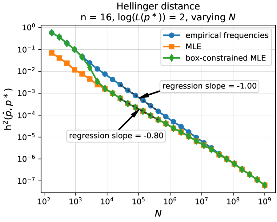
By construction, θ~~𝜃\tilde{\theta} is supermodular, so psuperscript𝑝p^{\ast} is MTP2subscriptMTP2\mathrm{MTP}_{2}, and log(L(p))=log(L)𝐿superscript𝑝𝐿\log(L(p^{\ast}))=\log(L). We sample N𝑁N i.i.d. observations {Zk}k=1Nsuperscriptsubscriptsubscript𝑍𝑘𝑘1𝑁\{Z_{k}\}_{k=1}^{N} from p𝑝p and form the matrix Y𝑌Y as in (2.2). We consider three estimators for psuperscript𝑝p^{\ast}: the empirical frequency matrix Y/N𝑌𝑁Y/N, the MLE given by (2.5), and the box-constrained estimator in (2.8). The latter two estimators are computed by variants of Algorithm 3. Note that in cases where some of the entries in the frequency matrix are zero, we cannot take logarithms and thus report Y/N𝑌𝑁Y/N as the output of the box-constrained estimator, while the unconstrained MLE can be calculated as in Section 4 above. For the unconstrained MLE, we do observe numerical instabilities when the number of observations is very low, eventually leading to underflows in the calculation. This can be remedied by imposing mild lower bounds on the resulting density, see Appendix C.2.
Refer to caption
(a) Varying N𝑁N, log(L(p))=2𝐿superscript𝑝2\log(L(p^{\ast}))=2
Refer to caption
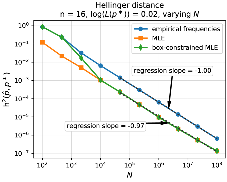
(b) Varying N𝑁N, log(L(p))=0.02𝐿superscript𝑝0.02\log(L(p^{\ast}))=0.02
Refer to caption
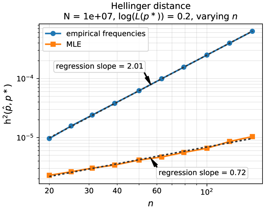
(c) Varying n𝑛n, log(L(p))=0.2𝐿superscript𝑝0.2\log(L(p^{\ast}))=0.2
Refer to caption
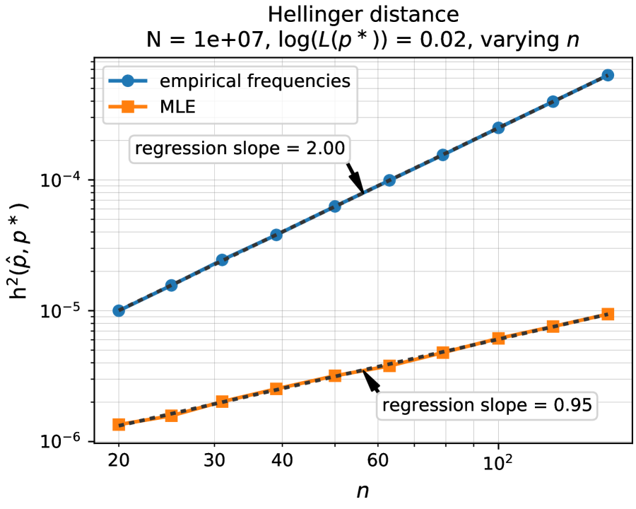
(d) Varying n𝑛n, log(L(p))=0.02𝐿superscript𝑝0.02\log(L(p^{\ast}))=0.02
Figure 2: Estimation of a density on a grid

In Figure 2, we plot the squared Hellinger distance 𝗁2(p,p^)superscript𝗁2superscript𝑝^𝑝\operatorname{\mathsf{h}}^{2}(p^{\ast},\hat{p}) for the three estimators in four setups, averaged over 20 independent replicates. More specifically, we report the results of linearly regressing the logarithms of the distances on the logarithms of the varying parameters over one or more manually selected ranges, corresponding to an estimate of the polynomial dependence on the parameter in question.

In Figures 2(a) and 2(b), we vary the sample size N𝑁N and keep n=16𝑛16n=16 fixed for log(L(p)){2,0.02}𝐿superscript𝑝20.02\log(L(p^{\ast}))\in\{2,0.02\}, respectively, while in Figures 2(c) and 2(d), we vary the grid size n𝑛n and keep N=𝑁absentN= 10,000,000 fixed for log(L(p)){0.2,0.02}𝐿superscript𝑝0.20.02\log(L(p^{\ast}))\in\{0.2,0.02\}, respectively. We observe that all three estimators achieve an N1superscript𝑁1N^{-1} asymptotic rate in Figure 2(a). Moreover, the box-constrained estimator (2.8) and the regular MLE (2.5) show very similar performance: For small N𝑁N, the probability for zero entries in Y/N𝑌𝑁Y/N is high and thus Y/N𝑌𝑁Y/N is used instead of the box-constrained estimator as explained in the above paragraph, which explains that its performance coincides with that of the empirical frequency matrix in this regime, while the MLE performs better because the dominant factor in this regime is n/N𝑛𝑁n/N. For an intermediate regime of N𝑁N, the estimation performance of the MLE and the box-constraint estimator is consistently better than that of Y/N𝑌𝑁Y/N, but it is attenuated once the (log(L(p))n/N)2/3superscript𝐿superscript𝑝𝑛𝑁23(\log(L(p^{\ast}))\,n/N)^{2/3} rate becomes active, which can be seen in Figure 2(a). On the other hand, in Figure 2(b), N𝑁N is not large enough relative to log(L(p))𝐿superscript𝑝\log(L(p^{\ast})) to capture this regime. Finally, for very large values of N𝑁N, the performance of all three estimators coincides, which for the box-constraint estimator matches the proof of the upper bound (up to logarithmic factors), see Remark 12.

A similar behavior can be seen in Figures 2(c) and 2(d), where the performance of the frequency matrix scales with n2superscript𝑛2n^{2}, while the regular MLE scales approximately like n2/3superscript𝑛23n^{2/3} (regression coefficient of 0.72) for a larger value of log(L(p))𝐿superscript𝑝\log(L(p^{\ast})) and like n𝑛n (regression coefficient of 0.95) when log(L(p))𝐿superscript𝑝\log(L(p^{\ast})) is small. Note that the performance of the box-constrained estimator is not plotted here since it mostly coincides with that of the regular MLE.
Refer to caption
(a) Varying N𝑁N
Refer to caption
(b) Varying n𝑛n
Figure 3: Runtimes for density on grid

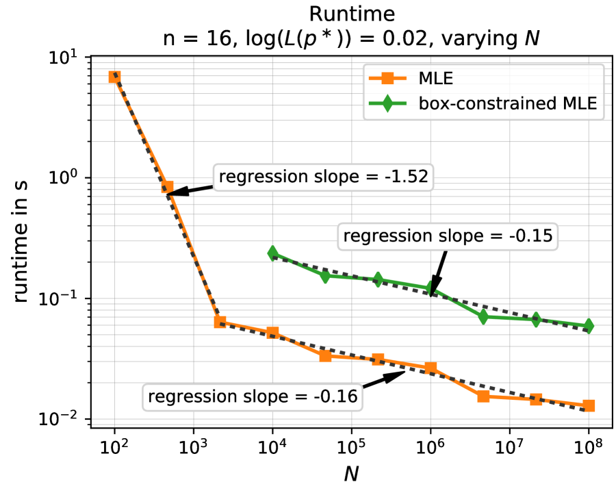
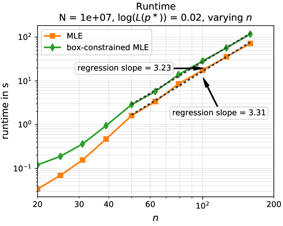
To investigate the practical performance of the proposed algorithms, in Figures 3, we report the runtime averaged over 20 replicates on an AMD 3400G desktop processor. Here, as well as in the previous examples, we stopped Algorithm 2 when a relative change in 2superscript2\ell^{2}-norm of less than 106superscript10610^{-6} was detected. Similarly, Algorithm 3 was stopped at a relative accuracy of 105superscript10510^{-5}. In Figure 3(a), we observe that the conditioning of the problem improves with larger sample sizes N𝑁N and deteriorates for small values of N𝑁N, leading to a decay in runtime of approximately N1.52superscript𝑁1.52N^{-1.52} up to N1,000𝑁1000N\approx 1,000, followed by a milder dependence of N0.15superscript𝑁0.15N^{-0.15} for larger values of N𝑁N. Note that the runtime for the boxed estimator is only plotted for N10,000𝑁10000N\geq 10,000 because of the presence of zeros in the empirical frequency matrix for smaller values of N𝑁N.

In Figure 3(b), we see that, as expected from a Dykstra-type algorithm, the conditioning of the problem worsens with increasing n𝑛n, necessitating more iterations and thus leading to an increase of runtime until convergence that is larger than the cost of one iteration, which is of order n2superscript𝑛2n^{2}. However, it is still reasonably mild, scaling roughly like n3.3superscript𝑛3.3n^{3.3} for larger values of n𝑛n. Overall, this highlights the practicability of the proposed algorithm for problems of medium size: Instances with n50𝑛50n\approx 50 can be solved within four seconds, while problems of size n=160𝑛160n=160 take under two minutes. Moreover, adding the additional box constraint (2.6) only slightly increases the runtime when n𝑛n is large.

5.2 Experiments for continuous density estimation

We consider the multivariate Gaussian distribution P=N(μ,Σ)superscript𝑃𝑁superscript𝜇superscriptΣP^{\ast}=N(\mu^{\ast},\Sigma^{\ast}) with parameters

μ=(0.50.5),Σ=(0.20.10.10.2),formulae-sequencesuperscript𝜇matrix0.50.5superscriptΣmatrix0.20.10.10.2\mu^{\ast}=\begin{pmatrix}0.5\\ 0.5\end{pmatrix},\quad\Sigma^{\ast}=\begin{pmatrix}0.2&0.1\\ 0.1&0.2\end{pmatrix}, (5.3)

conditioned on the event that Z[0,1]2𝑍superscript012Z\in[0,1]^{2} where ZPsimilar-to𝑍superscript𝑃Z\sim P^{\ast}. In other words, we consider the density

ρ(x)=1[0,1]2ρ~(y)dyρ~(x),x[0,1]2,formulae-sequencesuperscript𝜌𝑥1subscriptsuperscript012~𝜌𝑦differential-d𝑦~𝜌𝑥𝑥superscript012\rho^{\ast}(x)=\frac{1}{\int_{[0,1]^{2}}\tilde{\rho}(y)\,\mathrm{d}y}\tilde{\rho}(x),\quad x\in[0,1]^{2}, (5.4)

where

ρ~(x)=12π0.03exp(103((x10.5)2+(x20.5)2(x10.5)(x20.5))).~𝜌𝑥12𝜋0.03103superscriptsubscript𝑥10.52superscriptsubscript𝑥20.52subscript𝑥10.5subscript𝑥20.5\tilde{\rho}(x)=\frac{1}{2\pi\sqrt{0.03}}\exp\left(-\frac{10}{3}\left((x_{1}-0.5)^{2}+(x_{2}-0.5)^{2}-(x_{1}-0.5)(x_{2}-0.5)\right)\right). (5.5)
Refer to caption
(a) Comparison between empirical frequencies and MTP2subscriptMTP2\mathrm{MTP}_{2} estimator, oracle choice of n𝑛n
Refer to caption
(b) Variance part of the error when varying the scaling of n𝑛n
Figure 4: Performance of continuous density estimation
Refer to caption
(a) Ground truth ρsuperscript𝜌\rho^{\ast}
Refer to caption
(b) Approximation via frequencies Y/N𝑌𝑁Y/N
Refer to caption
(c) Approximation via MLE ρ^^𝜌\hat{\rho}
Figure 5: Visual comparison of continuous density estimation

Note that on [0,1]2superscript012[0,1]^{2}, ρCsuperscript𝜌superscript𝐶\rho^{\ast}\in C^{\infty} and that it is MTP2subscriptMTP2\mathrm{MTP}_{2}, which can be easily checked by computing the mixed derivative 12subscript1subscript2\partial_{1}\partial_{2} of the log-density. Here, we use it to evaluate the performance of the gridding strategy from Section 3.1 for both an oracle choice of n𝑛n, that is, exploiting the knowledge of the ground truth to pick the best possible value of n𝑛n from a given list, and a fixed scaling of n𝑛n in the cases β{0.5,0.75,1.0}𝛽0.50.751.0\beta\in\{0.5,0.75,1.0\}.

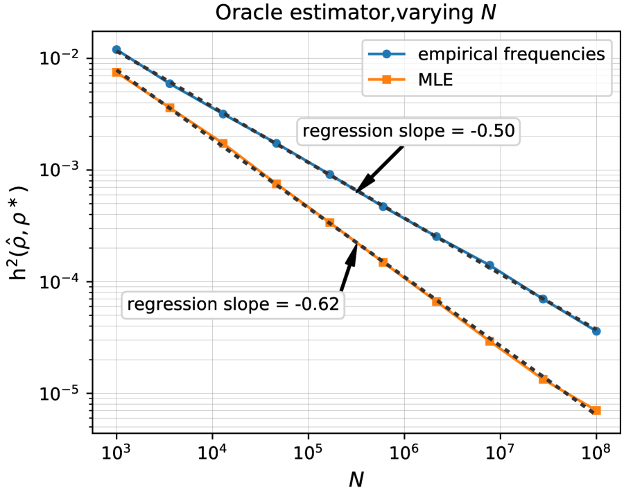
First, in Figure 4(a), with a varying number of i.i.d. observations {Zk}k=1Nsuperscriptsubscriptsubscript𝑍𝑘𝑘1𝑁\{Z_{k}\}_{k=1}^{N} from Psuperscript𝑃P^{\ast}, we plot the squared Hellinger distance 𝗁2(ρ^,ρ)superscript𝗁2^𝜌superscript𝜌\operatorname{\mathsf{h}}^{2}(\hat{\rho},\rho^{\ast}) for the estimator in (3.8), where n𝑛n is picked from 10 logarithmically spaced values between n=4𝑛4n=4 and n=200𝑛200n=200 according to which yields the smallest Hellinger distance, and for a similarly defined estimator where p^^𝑝\hat{p} is replaced by the empirical frequency matrix Y/N𝑌𝑁Y/N. We observe that the empirical frequency matrix achieves a rate of about N1/2superscript𝑁12N^{-1/2}, corresponding to the rate for general Hölder functions in 2D with β=1𝛽1\beta=1, while the MTP2subscriptMTP2\mathrm{MTP}_{2} MLE comes close to the predicted N2/3superscript𝑁23N^{-2/3} rate that corresponds to the β[1,2)𝛽12\beta\in[1,2) range (regression coefficient of 0.620.620.62).

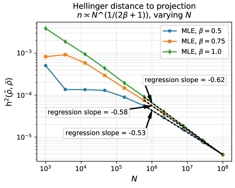
Second, to investigate the effect of different β𝛽\beta, in Figure 4(b), we use a fixed scaling n=CN1/(2β+1)𝑛𝐶superscript𝑁12𝛽1n=CN^{1/(2\beta+1)}. Note that we cannot expect to observe the rates in Theorem 6 when considering the distance 𝗁2(ρ^,ρ)superscript𝗁2^𝜌superscript𝜌\operatorname{\mathsf{h}}^{2}(\hat{\rho},\rho^{\ast}) in this setup since ρsuperscript𝜌\rho^{\ast} is Csuperscript𝐶C^{\infty}-smooth. Denoting by ρ¯¯𝜌\bar{\rho} the piecewise constant approximation to ρsuperscript𝜌\rho^{\ast} (see (6.81) below), this is due to the fact that the bias term 𝗁2(ρ¯,ρ)superscript𝗁2¯𝜌superscript𝜌\operatorname{\mathsf{h}}^{2}(\bar{\rho},\rho^{\ast}) could dominate the overall error 𝗁2(ρ^,ρ)superscript𝗁2^𝜌superscript𝜌\operatorname{\mathsf{h}}^{2}(\hat{\rho},\rho^{\ast}). Hence, we only plot the Hellinger distance corresponding to the variance part 𝗁2(ρ^,ρ¯)superscript𝗁2^𝜌¯𝜌\operatorname{\mathsf{h}}^{2}(\hat{\rho},\bar{\rho}). For computational reasons, C𝐶C is chosen for each β𝛽\beta so that for N=108𝑁superscript108N=10^{8}, we have n=200𝑛200n=200. Due to the similarities between the regular MLE and its box-constrained version observed in the previous section, all calculations were performed using the regular MLE, (2.5), resulting in slightly faster computations.

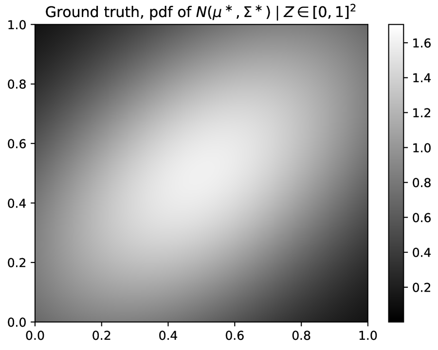
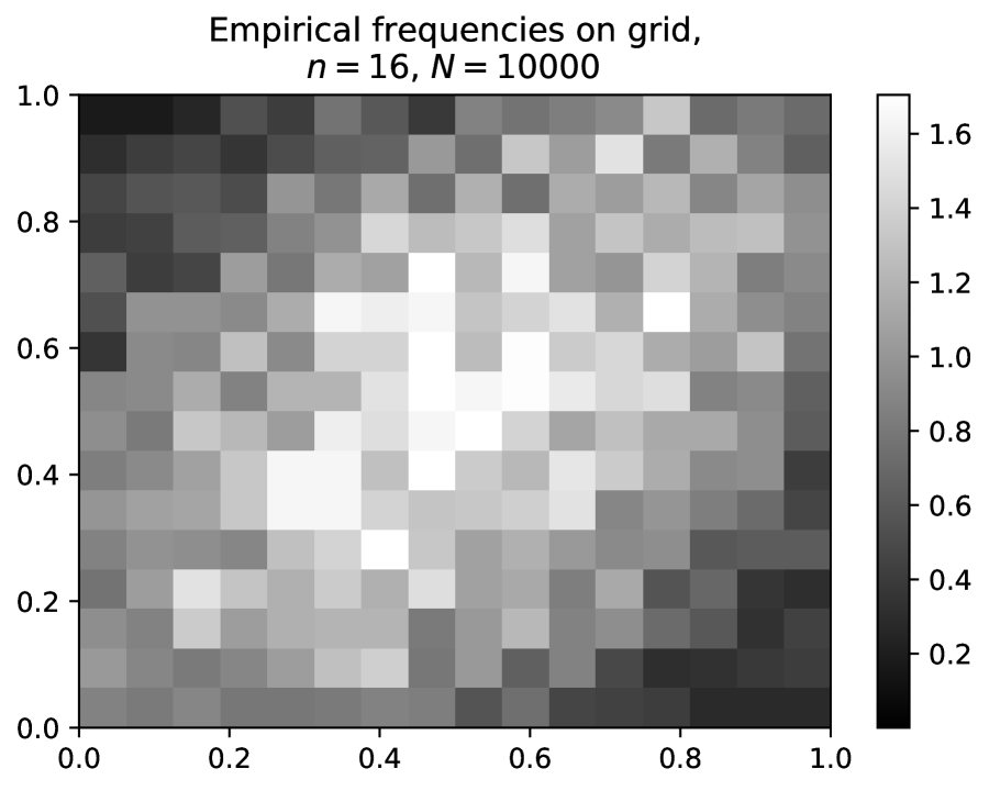
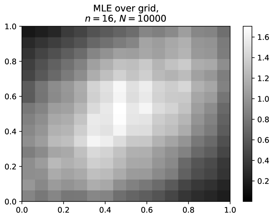
Performing linear regression on the doubly logarithmic plot for large values of N𝑁N, we observe rates of 0.530.530.53, 0.580.580.58, and 0.620.620.62 for β=0.5,0.75,1.0𝛽0.50.751.0\beta=0.5,0.75,1.0, respectively. These are close to 0.50.50.5, 0.60.60.6, and 2/3232/3, respectively, as predicted by Theorem 6. Additionally, we present heat maps of the density ρsuperscript𝜌\rho^{\ast} (Figure 5(a)), as well as an approximation via the frequncy matrix Y/N𝑌𝑁Y/N (Figure 5(b)) and the MLE (Figure 5(c)) for N=𝑁absentN= 10,000 and n=16𝑛16n=16. The visual smoothing effect of the MLE is quite obvious in this case.

6 Proofs

The proofs of our results are provided in this section. We first prove the upper bounds Theorems 3 and 6 in the discrete and smooth cases respectively, and then the lower bounds Theorems 4 and 7. In the proofs, we make use of the well-known relation [32, Lemma 7.23] that for PMFs p𝑝p and q𝑞q on 𝒳=[n1]×[n2]𝒳delimited-[]subscript𝑛1delimited-[]subscript𝑛2\mathcal{X}=[n_{1}]\times[n_{2}] or [0,1]2superscript012[0,1]^{2},

2𝗁2(p,q)𝖪𝖫(p,q)2(2+log(maxx𝒳p(x)q(x)))𝗁2(p,q).2superscript𝗁2𝑝𝑞𝖪𝖫𝑝𝑞22subscript𝑥𝒳𝑝𝑥𝑞𝑥superscript𝗁2𝑝𝑞\displaystyle 2\operatorname{\mathsf{h}}^{2}(p,q)\leq\operatorname{\mathsf{KL}}(p,q)\leq 2\Big{(}2+\log\big{(}\max_{x\in\mathcal{X}}\frac{p(x)}{q(x)}\big{)}\Big{)}\operatorname{\mathsf{h}}^{2}(p,q). (6.1)

6.1 Proof of Theorem 3

6.1.1 Setup of the proof: quadratic approximation

Let us define ε:=YNpassign𝜀𝑌𝑁superscript𝑝\varepsilon:=\frac{Y}{N}-p^{\ast}. Denote by 𝒜1subscript𝒜1\mathcal{A}_{1} the event of probability 12δ12𝛿1-2\delta that the bounds in Lemma 2 hold. On this event, θsuperscript𝜃\theta^{\ast} lies in the cube 𝒞(Y)𝒞𝑌\mathcal{C}(Y) defined in (2.6), so we have

1NY,θ~i,jeθ~i,j1NY,θ1,1𝑁𝑌~𝜃subscript𝑖𝑗superscript𝑒subscript~𝜃𝑖𝑗1𝑁𝑌superscript𝜃1\frac{1}{N}\langle Y,\tilde{\theta}\rangle-\sum_{i,j}e^{\tilde{\theta}_{i,j}}\geq\frac{1}{N}\langle Y,\theta^{\ast}\rangle-1,

which is equivalent to

p,θθ~+i,jeθ~i,j1ε,θ~θ.superscript𝑝superscript𝜃~𝜃subscript𝑖𝑗superscript𝑒subscript~𝜃𝑖𝑗1𝜀~𝜃superscript𝜃\displaystyle\langle p^{\ast},\theta^{\ast}-\tilde{\theta}\rangle+\sum_{i,j}e^{\tilde{\theta}_{i,j}}-1\leq\langle\varepsilon,\tilde{\theta}-\theta^{\ast}\rangle. (6.2)

In addition, the definition of 𝒞(Y)𝒞𝑌\mathcal{C}(Y) yields that |θ~i,jθi,j|log2log23<1.1subscript~𝜃𝑖𝑗subscriptsuperscript𝜃𝑖𝑗2231.1|\tilde{\theta}_{i,j}-\theta^{\ast}_{i,j}|\leq\log 2-\log\frac{2}{3}<1.1 for all i,j𝑖𝑗i,j.

By a quadratic Taylor approximation of eysuperscript𝑒𝑦e^{y}, it holds for x0𝑥0x\leq 0 and |yx|1.1𝑦𝑥1.1|y-x|\leq 1.1 that

ex+ex(yx)+ex(yx)2/4eyex+ex(yx)+2ex(yx)2.superscript𝑒𝑥superscript𝑒𝑥𝑦𝑥superscript𝑒𝑥superscript𝑦𝑥24superscript𝑒𝑦superscript𝑒𝑥superscript𝑒𝑥𝑦𝑥2superscript𝑒𝑥superscript𝑦𝑥2\displaystyle e^{x}+e^{x}(y-x)+e^{x}(y-x)^{2}/4\leq e^{y}\leq e^{x}+e^{x}(y-x)+2\,e^{x}(y-x)^{2}. (6.3)

Applying this approximation to the exponential terms of the left-hand side of (6.2), we obtain

p,θθ~+i,jeθi,j+i,jeθi,j(θ~i,jθi,j)+14i,jeθi,j(θ~i,jθi,j)21superscript𝑝superscript𝜃~𝜃subscript𝑖𝑗superscript𝑒subscriptsuperscript𝜃𝑖𝑗subscript𝑖𝑗superscript𝑒subscriptsuperscript𝜃𝑖𝑗subscript~𝜃𝑖𝑗subscriptsuperscript𝜃𝑖𝑗14subscript𝑖𝑗superscript𝑒subscriptsuperscript𝜃𝑖𝑗superscriptsubscript~𝜃𝑖𝑗subscriptsuperscript𝜃𝑖𝑗21\displaystyle\langle p^{\ast},\theta^{\ast}-\tilde{\theta}\rangle+\sum_{i,j}e^{\theta^{\ast}_{i,j}}+\sum_{i,j}e^{\theta^{\ast}_{i,j}}(\tilde{\theta}_{i,j}-\theta^{\ast}_{i,j})+\frac{1}{4}\sum_{i,j}e^{\theta^{\ast}_{i,j}}(\tilde{\theta}_{i,j}-\theta^{\ast}_{i,j})^{2}-1
p,θθ~+i,jeθ~i,j1absentsuperscript𝑝superscript𝜃~𝜃subscript𝑖𝑗superscript𝑒subscript~𝜃𝑖𝑗1\displaystyle\leq\langle p^{\ast},\theta^{\ast}-\tilde{\theta}\rangle+\sum_{i,j}e^{\tilde{\theta}_{i,j}}-1
p,θθ~+i,jeθi,j+i,jeθi,j(θ~i,jθi,j)+2i,jeθi,j(θ~i,jθi,j)21,absentsuperscript𝑝superscript𝜃~𝜃subscript𝑖𝑗superscript𝑒subscriptsuperscript𝜃𝑖𝑗subscript𝑖𝑗superscript𝑒subscriptsuperscript𝜃𝑖𝑗subscript~𝜃𝑖𝑗subscriptsuperscript𝜃𝑖𝑗2subscript𝑖𝑗superscript𝑒subscriptsuperscript𝜃𝑖𝑗superscriptsubscript~𝜃𝑖𝑗subscriptsuperscript𝜃𝑖𝑗21\displaystyle\leq\langle p^{\ast},\theta^{\ast}-\tilde{\theta}\rangle+\sum_{i,j}e^{\theta^{\ast}_{i,j}}+\sum_{i,j}e^{\theta^{\ast}_{i,j}}(\tilde{\theta}_{i,j}-\theta^{\ast}_{i,j})+2\sum_{i,j}e^{\theta^{\ast}_{i,j}}(\tilde{\theta}_{i,j}-\theta^{\ast}_{i,j})^{2}-1,

or equivalently,

14i,jpi,j(θ~i,jθi,j)2p,θθ~+i,jeθ~i,j12i,jpi,j(θ~i,jθi,j)2.14subscript𝑖𝑗subscriptsuperscript𝑝𝑖𝑗superscriptsubscript~𝜃𝑖𝑗subscriptsuperscript𝜃𝑖𝑗2superscript𝑝superscript𝜃~𝜃subscript𝑖𝑗superscript𝑒subscript~𝜃𝑖𝑗12subscript𝑖𝑗subscriptsuperscript𝑝𝑖𝑗superscriptsubscript~𝜃𝑖𝑗subscriptsuperscript𝜃𝑖𝑗2\displaystyle\frac{1}{4}\sum_{i,j}p^{\ast}_{i,j}(\tilde{\theta}_{i,j}-\theta^{\ast}_{i,j})^{2}\leq\langle p^{\ast},\theta^{\ast}-\tilde{\theta}\rangle+\sum_{i,j}e^{\tilde{\theta}_{i,j}}-1\leq 2\sum_{i,j}p^{\ast}_{i,j}(\tilde{\theta}_{i,j}-\theta^{\ast}_{i,j})^{2}. (6.4)

The rest of the proof hinges on this quadratic approximation. Particularly, it follows from (6.2) and (6.4) that

14i,jpi,j(θ~i,jθi,j)2ε,θ~θ.14subscript𝑖𝑗subscriptsuperscript𝑝𝑖𝑗superscriptsubscript~𝜃𝑖𝑗subscriptsuperscript𝜃𝑖𝑗2𝜀~𝜃superscript𝜃\displaystyle\frac{1}{4}\sum_{i,j}p^{\ast}_{i,j}(\tilde{\theta}_{i,j}-\theta^{\ast}_{i,j})^{2}\leq\langle\varepsilon,\tilde{\theta}-\theta^{\ast}\rangle. (6.5)

The main task in the sequel is to bound the right-hand side of (6.5). The strategy builds upon a spectral decomposition technique from the paper [19] on Monge matrix estimation.

6.1.2 Spectral decomposition of the difference operator

Recall the difference operator D𝐷D defined in (2.3) and D~~𝐷\tilde{D} defined analogously for dimension n2subscript𝑛2n_{2}. Throughout the proof, whenever we introduce notation in dimension n1subscript𝑛1n_{1}, the analogous one in dimension n2subscript𝑛2n_{2} is denoted by the same symbol with a tilde. We will decompose the noise ε𝜀\varepsilon in (6.5) according to a spectral decomposition of D𝐷D, so let us recall some basic facts about the matrix D𝐷D.

Denote the singular value decomposition of D𝐷D by

D=UΣW,U(n11)×(n11),Σ(n11)×n1,Wn1×n1formulae-sequence𝐷𝑈Σsuperscript𝑊topformulae-sequence𝑈superscriptsubscript𝑛11subscript𝑛11formulae-sequenceΣsuperscriptsubscript𝑛11subscript𝑛1𝑊superscriptsubscript𝑛1subscript𝑛1D=U\Sigma W^{\top},\quad U\in\mathbbm{R}^{(n_{1}-1)\times(n_{1}-1)},\quad\Sigma\in\mathbbm{R}^{(n_{1}-1)\times n_{1}},\quad W\in\mathbbm{R}^{n_{1}\times n_{1}} (6.6)

where we order the non-zero singular values of D𝐷D in ΣΣ\Sigma in ascending magnitude, so that the last column of W𝑊W spans the null-space of D𝐷D. In addition, we write W=[w1wn1].𝑊matrixsubscript𝑤1subscript𝑤subscript𝑛1W=\begin{bmatrix}w_{1}&\cdots&w_{n_{1}}\end{bmatrix}. Let us define a set of double indices

J:={(l,r)[n1]×[n2]:lrk}([n1]×{n2})({n1}×[n2]),assign𝐽conditional-set𝑙𝑟delimited-[]subscript𝑛1delimited-[]subscript𝑛2𝑙𝑟𝑘delimited-[]subscript𝑛1subscript𝑛2subscript𝑛1delimited-[]subscript𝑛2J:=\big{\{}(l,r)\in[n_{1}]\times[n_{2}]:lr\leq k\big{\}}\cup\big{(}[n_{1}]\times\{n_{2}\}\big{)}\cup\big{(}\{n_{1}\}\times[n_{2}]\big{)}, (6.7)

and set Jc=([n1]×[n2])Jsuperscript𝐽𝑐delimited-[]subscript𝑛1delimited-[]subscript𝑛2𝐽J^{c}=([n_{1}]\times[n_{2}])\setminus J.

We introduce a projection operator Π:n1×n2n1×n2:Πsuperscriptsubscript𝑛1subscript𝑛2superscriptsubscript𝑛1subscript𝑛2\Pi:\mathbbm{R}^{n_{1}\times n_{2}}\to\mathbbm{R}^{n_{1}\times n_{2}}, defined as the projection onto the linear span of {wiw~j:(i,j)Jc}conditional-setsubscript𝑤𝑖superscriptsubscript~𝑤𝑗top𝑖𝑗superscript𝐽𝑐\{w_{i}\tilde{w}_{j}^{\top}:(i,j)\in J^{c}\} that is orthogonal with respect to the inner product

A,B1/p:=i,j1pi,jAi,jBi,j.assignsubscript𝐴𝐵1superscript𝑝subscript𝑖𝑗1subscriptsuperscript𝑝𝑖𝑗subscript𝐴𝑖𝑗subscript𝐵𝑖𝑗\langle A,B\rangle_{1/p^{\ast}}:=\sum_{i,j}\frac{1}{p^{\ast}_{i,j}}A_{i,j}B_{i,j}. (6.8)

In particular, there exists an orthonormal basis {V(l,r)n1×n2:(l,r)[n1]×[n2]}conditional-setsuperscript𝑉𝑙𝑟superscriptsubscript𝑛1subscript𝑛2𝑙𝑟delimited-[]subscript𝑛1delimited-[]subscript𝑛2\{V^{(l,r)}\in\mathbbm{R}^{n_{1}\times n_{2}}:(l,r)\in[n_{1}]\times[n_{2}]\} of n1×n2superscriptsubscript𝑛1subscript𝑛2\mathbbm{R}^{n_{1}\times n_{2}} with respect to the inner product .,.1/p\langle.,.\rangle_{1/p^{\ast}} such that

Π(A)=(l,r)JcV(l,r)V(l,r),A1/p and (IΠ)(A)=(l,r)JV(l,r)V(l,r),A1/p.formulae-sequenceΠ𝐴subscript𝑙𝑟superscript𝐽𝑐superscript𝑉𝑙𝑟subscriptsuperscript𝑉𝑙𝑟𝐴1superscript𝑝 and 𝐼Π𝐴subscript𝑙𝑟𝐽superscript𝑉𝑙𝑟subscriptsuperscript𝑉𝑙𝑟𝐴1superscript𝑝\Pi(A)=\sum_{(l,r)\in J^{c}}V^{(l,r)}\langle V^{(l,r)},A\rangle_{1/p^{\ast}}\quad\text{ and }\quad(I-\Pi)(A)=\sum_{(l,r)\in J}V^{(l,r)}\langle V^{(l,r)},A\rangle_{1/p^{\ast}}. (6.9)

To characterize these projection operators further, we introduce the following notation. Let direct-product\odot and \oslash denote entrywise multiplication and division respectively between matrices. With a slight abuse of notation, we use psuperscript𝑝\sqrt{p^{\ast}} and 1/p1superscript𝑝1/p^{\ast} to denote the entrywise square root and the entrywise inverse of psuperscript𝑝p^{\ast} respectively. Let ΛΛ\Lambda and Λ1superscriptΛ1\Lambda^{-1} be the scaling operators from n1×n2superscriptsubscript𝑛1subscript𝑛2\mathbbm{R}^{n_{1}\times n_{2}} to itself, defined by

Λ(A)=Λ𝐴absent\displaystyle\Lambda(A)={} Ap,tensor-product𝐴superscript𝑝\displaystyle A\otimes p^{\ast},\quad A𝐴absent\displaystyle A\in{} n1×n2,superscriptsubscript𝑛1subscript𝑛2\displaystyle\mathbbm{R}^{n_{1}\times n_{2}}, (6.10)
Λ1(A)=superscriptΛ1𝐴absent\displaystyle\Lambda^{-1}(A)={} Ap,𝐴superscript𝑝\displaystyle A\oslash p^{\ast},\quad A𝐴absent\displaystyle A\in{} n1×n2,superscriptsubscript𝑛1subscript𝑛2\displaystyle\mathbbm{R}^{n_{1}\times n_{2}}, (6.11)

respectively. Let \mathcal{L} be the linear operator from |Jc|superscriptsuperscript𝐽𝑐\mathbbm{R}^{|J^{c}|} (indexed by (l,r)Jc𝑙𝑟superscript𝐽𝑐(l,r)\in J^{c}) to n1×n2superscriptsubscript𝑛1subscript𝑛2\mathbbm{R}^{n_{1}\times n_{2}}, defined by

(B)=𝐵absent\displaystyle\mathcal{L}(B)={} (l,r)JcBl,rwlw~r,subscript𝑙𝑟superscript𝐽𝑐subscript𝐵𝑙𝑟subscript𝑤𝑙superscriptsubscript~𝑤𝑟top\displaystyle\sum_{(l,r)\in J^{c}}B_{l,r}w_{l}\tilde{w}_{r}^{\top},\quad B𝐵absent\displaystyle B\in{} |Jc|,superscriptsuperscript𝐽𝑐\displaystyle\mathbbm{R}^{|J^{c}|}, (6.12)

and denote by superscripttop\mathcal{L}^{\top} the transpose of \mathcal{L} with respect to the standard inner products in the corresponding spaces. In other words, we have

((A))l,r=wlw~r,A,(l,r)Jc,An1×n2.formulae-sequencesubscriptsuperscripttop𝐴𝑙𝑟subscript𝑤𝑙superscriptsubscript~𝑤𝑟top𝐴formulae-sequence𝑙𝑟superscript𝐽𝑐𝐴superscriptsubscript𝑛1subscript𝑛2(\mathcal{L}^{\top}(A))_{l,r}=\langle w_{l}\tilde{w}_{r}^{\top},A\rangle,\quad(l,r)\in J^{c},\quad A\in\mathbbm{R}^{n_{1}\times n_{2}}. (6.13)

The linear operators ΠΠ\Pi and ΛΛ\Lambda can be viewed as n1n2×n1n2subscript𝑛1subscript𝑛2subscript𝑛1subscript𝑛2n_{1}n_{2}\times n_{1}n_{2} matrices, while the linear operator \mathcal{L} can be seen as an n1n2×|Jc|subscript𝑛1subscript𝑛2superscript𝐽𝑐n_{1}n_{2}\times|J^{c}| matrix. Moreover, we have the following lemma whose proof is deferred to Section 6.1.6.

Lemma 9.

The smallest eigenvalue of the operator Λ1superscripttopsuperscriptΛ1\mathcal{L}^{\top}\Lambda^{-1}\mathcal{L} satisfies that

λmin(Λ1)1p𝗆𝖺𝗑.subscript𝜆superscripttopsuperscriptΛ11subscriptsuperscript𝑝𝗆𝖺𝗑\lambda_{\min}(\mathcal{L}^{\top}\Lambda^{-1}\mathcal{L})\geq\frac{1}{p^{\ast}_{\mathsf{max}}}. (6.14)

Moreover, ΠΠ\Pi can be written as

Π=(Λ1)1Λ1.ΠsuperscriptsuperscripttopsuperscriptΛ11superscripttopsuperscriptΛ1\Pi=\mathcal{L}(\mathcal{L}^{\top}\Lambda^{-1}\mathcal{L})^{-1}\mathcal{L}^{\top}\Lambda^{-1}. (6.15)

To control ϵ,θ~θitalic-ϵ~𝜃superscript𝜃\langle\epsilon,\tilde{\theta}-\theta^{\ast}\rangle on the right-hand side of (6.5), we decompose it as

ε,θ~θ=(IΠ)(ε),θ~θ+Π(ε),θ~θ.𝜀~𝜃superscript𝜃𝐼Π𝜀~𝜃superscript𝜃Π𝜀~𝜃superscript𝜃\displaystyle\langle\varepsilon,\tilde{\theta}-\theta^{\ast}\rangle=\langle(I-\Pi)(\varepsilon),\tilde{\theta}-\theta^{\ast}\rangle+\langle\Pi(\varepsilon),\tilde{\theta}-\theta^{\ast}\rangle. (6.16)

Before proceeding to bound these two terms separately, we state two lemmas whose proofs are deferred to Sections 6.1.7 and 6.1.8, respectively.

Lemma 10.

The image of the projection ΠΠ\Pi is included in the image of the map ADAD~maps-to𝐴superscript𝐷top𝐴~𝐷A\mapsto D^{\top}A\tilde{D}.

Lemma 11.

For any (i,j)[n1]×[n2]𝑖𝑗delimited-[]subscript𝑛1delimited-[]subscript𝑛2(i,j)\in[n_{1}]\times[n_{2}], we have that

(l,r)JcΣl,l2Σ~r,r2Ui,l2U~j,r2n1n2klog(n2).less-than-or-similar-tosubscript𝑙𝑟superscript𝐽𝑐superscriptsubscriptΣ𝑙𝑙2superscriptsubscript~Σ𝑟𝑟2superscriptsubscript𝑈𝑖𝑙2superscriptsubscript~𝑈𝑗𝑟2subscript𝑛1subscript𝑛2𝑘subscript𝑛2\sum_{(l,r)\in J^{c}}\Sigma_{l,l}^{-2}\tilde{\Sigma}_{r,r}^{-2}U_{i,l}^{2}\tilde{U}_{j,r}^{2}\lesssim\frac{n_{1}n_{2}}{k}\log(n_{2}).

6.1.3 Bounding the first term in (6.16)

By Hölder’s inequality,

(IΠ)(ε),θ~θ=(IΠ)(ε)p,(θ~θ)p(IΠ)(ε)1/pθ~θp.𝐼Π𝜀~𝜃superscript𝜃𝐼Π𝜀superscript𝑝direct-product~𝜃superscript𝜃superscript𝑝subscriptnorm𝐼Π𝜀1superscript𝑝subscriptnorm~𝜃superscript𝜃superscript𝑝\displaystyle\langle(I-\Pi)(\varepsilon),\tilde{\theta}-\theta^{\ast}\rangle=\big{\langle}(I-\Pi)(\varepsilon)\oslash\sqrt{p^{\ast}},(\tilde{\theta}-\theta^{\ast})\odot\sqrt{p^{\ast}}\,\big{\rangle}\leq\|(I-\Pi)(\varepsilon)\|_{1/p^{\ast}}\|\tilde{\theta}-\theta^{\ast}\|_{p^{\ast}}. (6.17)

Now we focus on the quantity (IΠ)(ε)1/psubscriptnorm𝐼Π𝜀1superscript𝑝\|(I-\Pi)(\varepsilon)\|_{1/p^{\ast}}. By the definition of ΠΠ\Pi and the orthogonality condition that V(l,r),V(l,r)=0superscript𝑉𝑙𝑟superscript𝑉superscript𝑙superscript𝑟0\langle V^{(l,r)},V^{(l^{\prime},r^{\prime})}\rangle=0 for any (l,r)(l,r)𝑙𝑟superscript𝑙superscript𝑟(l,r)\neq(l^{\prime},r^{\prime}), we obtain that

(IΠ)(ε)1/p2superscriptsubscriptnorm𝐼Π𝜀1superscript𝑝2\displaystyle\|(I-\Pi)(\varepsilon)\|_{1/p^{\ast}}^{2} =(l,r)JV(l,r)V(l,r),ϵ1/p1/p2absentsuperscriptsubscriptnormsubscript𝑙𝑟𝐽superscript𝑉𝑙𝑟subscriptsuperscript𝑉𝑙𝑟italic-ϵ1superscript𝑝1superscript𝑝2\displaystyle=\Big{\|}\sum_{(l,r)\in J}V^{(l,r)}\langle V^{(l,r)},\epsilon\rangle_{1/p^{\ast}}\Big{\|}_{1/p^{\ast}}^{2} (6.18)
=(l,r)JV(l,r),ϵ1/p2|J|max(l,r)J(V(l,r),ϵ1/p)2.\displaystyle=\sum_{(l,r)\in J}\langle V^{(l,r)},\epsilon\rangle_{1/p^{\ast}}^{2}\leq|J|\max_{(l,r)\in J}(\langle V^{(l,r)},\epsilon\rangle_{1/p^{\ast}})^{2}. (6.19)

Note that we can write

V(l,r),ϵ1/p=1NV(l,r)p,Nε.subscriptsuperscript𝑉𝑙𝑟italic-ϵ1superscript𝑝1𝑁superscript𝑉𝑙𝑟superscript𝑝𝑁𝜀\displaystyle\langle V^{(l,r)},\epsilon\rangle_{1/p^{\ast}}=\big{\langle}\frac{1}{N}V^{(l,r)}\oslash p^{\ast},N\varepsilon\big{\rangle}. (6.20)

Recall that Y𝑌Y has the multinomial distribution 𝖬𝗎𝗅𝗍𝗂(N,p)𝖬𝗎𝗅𝗍𝗂𝑁superscript𝑝\mathsf{Multi}(N,p^{*}), and Nε=YNp𝑁𝜀𝑌𝑁superscript𝑝N\varepsilon=Y-Np^{\ast} is the deviation of Y𝑌Y from its mean. Therefore, Lemma 18 yields that on an event 𝒜2subscript𝒜2\mathcal{A}_{2} of probability 1δ1𝛿1-\delta,

max(l,r)J|V(l,r),ϵ1/p|subscript𝑙𝑟𝐽subscriptsuperscript𝑉𝑙𝑟italic-ϵ1superscript𝑝\displaystyle\max_{(l,r)\in J}|\langle V^{(l,r)},\epsilon\rangle_{1/p^{\ast}}|
less-than-or-similar-to\displaystyle\lesssim{} (max(l,r)J1NV(l,r)pNp)log(|J|/δ)+(max(l,r)J1NV(l,r)p)log(|J|/δ).subscript𝑙𝑟𝐽subscriptnorm1𝑁superscript𝑉𝑙𝑟superscript𝑝𝑁superscript𝑝𝐽𝛿subscript𝑙𝑟𝐽subscriptnorm1𝑁superscript𝑉𝑙𝑟superscript𝑝𝐽𝛿\displaystyle\Big{(}\max_{(l,r)\in J}\Big{\|}\frac{1}{N}V^{(l,r)}\oslash p^{\ast}\Big{\|}_{Np^{\ast}}\Big{)}\sqrt{\log(|J|/\delta)}+\Big{(}\max_{(l,r)\in J}\Big{\|}\frac{1}{N}V^{(l,r)}\oslash p^{\ast}\Big{\|}_{\infty}\Big{)}\log(|J|/\delta). (6.21)

To bound the two norms above, we note that by orthogonality of the V(l,r)superscript𝑉𝑙𝑟V^{(l,r)} with respect to .,.1/p\langle.,.\rangle_{1/p^{\ast}},

1NV(l,r)pNp2=1NV(l,r)1/p2=1N.superscriptsubscriptnorm1𝑁superscript𝑉𝑙𝑟superscript𝑝𝑁superscript𝑝2superscriptsubscriptnorm1𝑁superscript𝑉𝑙𝑟1superscript𝑝21𝑁\displaystyle\Big{\|}\frac{1}{N}V^{(l,r)}\oslash p^{\ast}\Big{\|}_{Np^{\ast}}^{2}=\Big{\|}\frac{1}{\sqrt{N}}V^{(l,r)}\Big{\|}_{1/p^{\ast}}^{2}=\frac{1}{N}. (6.22)

In addition, it holds that

1NV(l,r)subscriptnorm1𝑁superscript𝑉𝑙𝑟absent\displaystyle\Big{\|}\frac{1}{N}V^{(l,r)}\Big{\|}_{\infty}\leq{} 1NV(l,r)F=1NNV(l,r)pNpsubscriptnorm1𝑁superscript𝑉𝑙𝑟𝐹subscriptnorm1𝑁𝑁superscript𝑉𝑙𝑟superscript𝑝𝑁superscript𝑝\displaystyle\Big{\|}\frac{1}{N}V^{(l,r)}\Big{\|}_{F}=\Big{\|}\frac{1}{N\sqrt{N}}V^{(l,r)}\oslash\sqrt{p^{\ast}}\Big{\|}_{Np^{\ast}} (6.23)
\displaystyle\leq{} 1Np𝗆𝗂𝗇1NV(l,r)Np=1Np𝗆𝗂𝗇1Nlog(n1/δ),1𝑁subscriptsuperscript𝑝𝗆𝗂𝗇subscriptnorm1𝑁superscript𝑉𝑙𝑟𝑁superscript𝑝1𝑁subscriptsuperscript𝑝𝗆𝗂𝗇1𝑁subscript𝑛1𝛿\displaystyle\frac{1}{\sqrt{Np^{\ast}_{\mathsf{min}}}}\Big{\|}\frac{1}{N}V^{(l,r)}\Big{\|}_{Np^{\ast}}=\frac{1}{N\sqrt{p^{\ast}_{\mathsf{min}}}}\leq\frac{1}{\sqrt{N\log(n_{1}/\delta)}}, (6.24)

where we used (6.22) and that N12log(n1n2/δ)/p𝗆𝗂𝗇𝑁12subscript𝑛1subscript𝑛2𝛿subscriptsuperscript𝑝𝗆𝗂𝗇N\geq 12\log(n_{1}n_{2}/\delta)/p^{\ast}_{\mathsf{min}} by assumption. Further, we can control the cardinality of J𝐽J by

n1|J|n1n2,and|J|=(l,r)J1n1+n21+r=1n2k/r2n1+klog(n2).formulae-sequencesubscript𝑛1𝐽subscript𝑛1subscript𝑛2and𝐽subscript𝑙𝑟𝐽1subscript𝑛1subscript𝑛21superscriptsubscript𝑟1subscript𝑛2𝑘𝑟2subscript𝑛1𝑘subscript𝑛2n_{1}\leq|J|\leq n_{1}n_{2},\quad\text{and}\quad|J|=\sum_{(l,r)\in J}1\leq n_{1}+n_{2}-1+\sum_{r=1}^{n_{2}}\lfloor k/r\rfloor\leq 2n_{1}+k\log(n_{2}). (6.25)

Combining (6.17), (6.19), (6.21), (6.22), (6.24) and (6.25), we see that on the event 𝒜2subscript𝒜2\mathcal{A}_{2},

(IΠ)(ε),θ~θ𝐼Π𝜀~𝜃superscript𝜃\displaystyle\langle(I-\Pi)(\varepsilon),\tilde{\theta}-\theta^{\ast}\rangle θ~θpn1+klog(n2)(log(n1/δ)N+log(n1/δ)Nlog(n1/δ))less-than-or-similar-toabsentsubscriptnorm~𝜃superscript𝜃superscript𝑝subscript𝑛1𝑘subscript𝑛2subscript𝑛1𝛿𝑁subscript𝑛1𝛿𝑁subscript𝑛1𝛿\displaystyle\lesssim\|\tilde{\theta}-\theta^{\ast}\|_{p^{\ast}}\sqrt{n_{1}+k\log(n_{2})}\Big{(}\sqrt{\frac{\log(n_{1}/\delta)}{N}}+\frac{\log(n_{1}/\delta)}{\sqrt{N\log(n_{1}/\delta)}}\Big{)} (6.26)
θ~θpn1log(n1/δ)+klog(n1/δ)log(n2)N.less-than-or-similar-toabsentsubscriptnorm~𝜃superscript𝜃superscript𝑝subscript𝑛1subscript𝑛1𝛿𝑘subscript𝑛1𝛿subscript𝑛2𝑁\displaystyle\lesssim\|\tilde{\theta}-\theta^{\ast}\|_{p^{\ast}}\sqrt{\frac{n_{1}\log(n_{1}/\delta)+k\log(n_{1}/\delta)\log(n_{2})}{N}}. (6.27)

6.1.4 Bounding the second term in (6.16)

By Lemma 10, the image of ΠΠ\Pi is included in the image of the adjoint map ADAD~maps-to𝐴superscript𝐷top𝐴~𝐷A\mapsto D^{\top}A\tilde{D}. Since AD(D)AD~D~maps-to𝐴superscript𝐷topsuperscriptsuperscript𝐷top𝐴superscript~𝐷~𝐷A\mapsto D^{\top}(D^{\top})^{\dagger}A\tilde{D}^{\dagger}\tilde{D} is the orthogonal projection onto this image, we thus have

Π(ε),θ~θ=Π𝜀~𝜃superscript𝜃absent\displaystyle\langle\Pi(\varepsilon),\tilde{\theta}-\theta^{\ast}\rangle={} D(D)Π(ε)D~D~,θ~θsuperscript𝐷topsuperscriptsuperscript𝐷topΠ𝜀superscript~𝐷~𝐷~𝜃superscript𝜃\displaystyle\langle D^{\top}(D^{\top})^{\dagger}\Pi(\varepsilon)\tilde{D}^{\dagger}\tilde{D},\tilde{\theta}-\theta^{\ast}\rangle (6.28)
=\displaystyle={} (D)Π(ε)D~,D(θ~θ)D~superscriptsuperscript𝐷topΠ𝜀superscript~𝐷𝐷~𝜃superscript𝜃superscript~𝐷top\displaystyle\langle(D^{\dagger})^{\top}\Pi(\varepsilon)\tilde{D}^{\dagger},D(\tilde{\theta}-\theta^{\ast})\tilde{D}^{\top}\rangle (6.29)
\displaystyle\leq{} (D)Π(ε)D~D(θ~θ)D~1subscriptnormsuperscriptsuperscript𝐷topΠ𝜀superscript~𝐷subscriptnorm𝐷~𝜃superscript𝜃superscript~𝐷top1\displaystyle\big{\|}(D^{\dagger})^{\top}\Pi(\varepsilon)\tilde{D}^{\dagger}\big{\|}_{\infty}\,\big{\|}D(\tilde{\theta}-\theta^{\ast})\tilde{D}^{\top}\big{\|}_{1} (6.30)

by Hölder’s inequality.

We first consider the term (D)Π(ε)D~subscriptnormsuperscriptsuperscript𝐷topΠ𝜀superscript~𝐷\big{\|}(D^{\dagger})^{\top}\Pi(\varepsilon)\tilde{D}^{\dagger}\big{\|}_{\infty}. By the formula (6.15) for ΠΠ\Pi and the singular value decomposition of D𝐷D, it holds that

(D)Π(ε)D~=superscriptsuperscript𝐷topΠ𝜀superscript~𝐷absent\displaystyle(D^{\dagger})^{\top}\Pi(\varepsilon)\tilde{D}^{\dagger}={} (l,r)JcΣl,l1Σr,r1U,lU~,rwlw~r,Π(ϵ)subscript𝑙𝑟superscript𝐽𝑐subscriptsuperscriptΣ1𝑙𝑙subscriptsuperscriptΣ1𝑟𝑟subscript𝑈𝑙superscriptsubscript~𝑈𝑟topsubscript𝑤𝑙superscriptsubscript~𝑤𝑟topΠitalic-ϵ\displaystyle\sum_{(l,r)\in J^{c}}\Sigma^{-1}_{l,l}\Sigma^{-1}_{r,r}U_{\cdot,l}\tilde{U}_{\cdot,r}^{\top}\langle w_{l}\tilde{w}_{r}^{\top},\Pi(\epsilon)\rangle (6.31)
=\displaystyle={} (l,r)JcΣl,l1Σr,r1U,lU~,rwlw~r,(Λ1)1Λ1(ϵ)subscript𝑙𝑟superscript𝐽𝑐subscriptsuperscriptΣ1𝑙𝑙subscriptsuperscriptΣ1𝑟𝑟subscript𝑈𝑙superscriptsubscript~𝑈𝑟topsubscript𝑤𝑙superscriptsubscript~𝑤𝑟topsuperscriptsuperscripttopsuperscriptΛ11superscripttopsuperscriptΛ1italic-ϵ\displaystyle\sum_{(l,r)\in J^{c}}\Sigma^{-1}_{l,l}\Sigma^{-1}_{r,r}U_{\cdot,l}\tilde{U}_{\cdot,r}^{\top}\langle w_{l}\tilde{w}_{r}^{\top},\mathcal{L}(\mathcal{L}^{\top}\Lambda^{-1}\mathcal{L})^{-1}\mathcal{L}^{\top}\Lambda^{-1}(\epsilon)\rangle (6.32)
=\displaystyle={} (l,r)JcΣl,l1Σr,r1U,lU~,rΛ1(Λ1)1(wlw~r),ϵ.subscript𝑙𝑟superscript𝐽𝑐subscriptsuperscriptΣ1𝑙𝑙subscriptsuperscriptΣ1𝑟𝑟subscript𝑈𝑙superscriptsubscript~𝑈𝑟topsuperscriptΛ1superscriptsuperscripttopsuperscriptΛ11superscripttopsubscript𝑤𝑙superscriptsubscript~𝑤𝑟topitalic-ϵ\displaystyle\sum_{(l,r)\in J^{c}}\Sigma^{-1}_{l,l}\Sigma^{-1}_{r,r}U_{\cdot,l}\tilde{U}_{\cdot,r}^{\top}\langle\Lambda^{-1}\mathcal{L}(\mathcal{L}^{\top}\Lambda^{-1}\mathcal{L})^{-1}\mathcal{L}^{\top}(w_{l}\tilde{w}_{r}^{\top}),\epsilon\rangle. (6.33)

By (6.13) and the orthogonality of the vectors {wl}l[n1]subscriptsubscript𝑤𝑙𝑙delimited-[]subscript𝑛1\{w_{l}\}_{l\in[n_{1}]} and {w~r}r[n2]subscriptsubscript~𝑤𝑟𝑟delimited-[]subscript𝑛2\{\tilde{w}_{r}\}_{r\in[n_{2}]}, we have that (wlw~r)=e(l,r)superscripttopsubscript𝑤𝑙superscriptsubscript~𝑤𝑟topsuperscript𝑒𝑙𝑟\mathcal{L}^{\top}(w_{l}\tilde{w}_{r}^{\top})=e^{(l,r)} if (l,r)Jc𝑙𝑟superscript𝐽𝑐(l,r)\in J^{c} and zero otherwise, where e(l,r)superscript𝑒𝑙𝑟e^{(l,r)} denotes the coordinate vector in |Jc|superscriptsuperscript𝐽𝑐\mathbbm{R}^{|J^{c}|} with a one in the (l,r)𝑙𝑟(l,r)th component and zero in all others. Hence, if we define a(i,j)|Jc|superscript𝑎𝑖𝑗superscriptsuperscript𝐽𝑐a^{(i,j)}\in\mathbbm{R}^{|J^{c}|} for (i,j)[n11]×[n21]𝑖𝑗delimited-[]subscript𝑛11delimited-[]subscript𝑛21(i,j)\in[n_{1}-1]\times[n_{2}-1] by

(a(i,j))l,r:=Σl,l1Σr,r1Ui,lU~j,r,assignsubscriptsuperscript𝑎𝑖𝑗𝑙𝑟superscriptsubscriptΣ𝑙𝑙1superscriptsubscriptΣ𝑟𝑟1subscript𝑈𝑖𝑙subscript~𝑈𝑗𝑟(a^{(i,j)})_{l,r}:=\Sigma_{l,l}^{-1}\Sigma_{r,r}^{-1}U_{i,l}\tilde{U}_{j,r}, (6.34)

then for (i,j)[n11]×[n21]𝑖𝑗delimited-[]subscript𝑛11delimited-[]subscript𝑛21(i,j)\in[n_{1}-1]\times[n_{2}-1], we obtain

((D)Π(ε)D~)i,j=subscriptsuperscriptsuperscript𝐷topΠ𝜀superscript~𝐷𝑖𝑗absent\displaystyle\left((D^{\dagger})^{\top}\Pi(\varepsilon)\tilde{D}^{\dagger}\right)_{i,j}={} (l,r)Jc(a(i,j))l,rΛ1(Λ1)1e(l,r),ϵsubscript𝑙𝑟superscript𝐽𝑐subscriptsuperscript𝑎𝑖𝑗𝑙𝑟superscriptΛ1superscriptsuperscripttopsuperscriptΛ11superscript𝑒𝑙𝑟italic-ϵ\displaystyle\sum_{(l,r)\in J^{c}}(a^{(i,j)})_{l,r}\langle\Lambda^{-1}\mathcal{L}(\mathcal{L}^{\top}\Lambda^{-1}\mathcal{L})^{-1}e^{(l,r)},\epsilon\rangle (6.35)
=\displaystyle={} 1NΛ1(Λ1)1a(i,j)=:B(i,j),Nϵ.subscript1𝑁superscriptΛ1superscriptsuperscripttopsuperscriptΛ11superscript𝑎𝑖𝑗:absentsuperscript𝐵𝑖𝑗𝑁italic-ϵ\displaystyle\langle\underbrace{\frac{1}{N}\Lambda^{-1}\mathcal{L}(\mathcal{L}^{\top}\Lambda^{-1}\mathcal{L})^{-1}a^{(i,j)}}_{=:B^{(i,j)}},N\epsilon\rangle. (6.36)

As before, Lemma 18 yields that on an event 𝒜3subscript𝒜3\mathcal{A}_{3} of probability 1δ1𝛿1-\delta,

(D)Π(ε)D~(maxi,jB(i,j)Np)log(n1/δ)+(maxi,jB(i,j))log(n1/δ).less-than-or-similar-tosubscriptnormsuperscriptsuperscript𝐷topΠ𝜀superscript~𝐷subscript𝑖𝑗subscriptnormsuperscript𝐵𝑖𝑗𝑁superscript𝑝subscript𝑛1𝛿subscript𝑖𝑗subscriptnormsuperscript𝐵𝑖𝑗subscript𝑛1𝛿\displaystyle\Big{\|}(D^{\dagger})^{\top}\Pi(\varepsilon)\tilde{D}^{\dagger}\Big{\|}_{\infty}\lesssim\Big{(}\max_{i,j}\big{\|}B^{(i,j)}\big{\|}_{Np^{\ast}}\Big{)}\sqrt{\log(n_{1}/\delta)}+\Big{(}\max_{i,j}\big{\|}B^{(i,j)}\big{\|}_{\infty}\Big{)}\log(n_{1}/\delta). (6.37)

We proceed to bound B(i,j)Npsubscriptnormsuperscript𝐵𝑖𝑗𝑁superscript𝑝\|B^{(i,j)}\|_{Np^{\ast}} and B(i,j)subscriptnormsuperscript𝐵𝑖𝑗\|B^{(i,j)}\|_{\infty}. First,

B(i,j)Np2=superscriptsubscriptnormsuperscript𝐵𝑖𝑗𝑁superscript𝑝2absent\displaystyle\Big{\|}B^{(i,j)}\Big{\|}_{Np^{\ast}}^{2}={} 1NΛ1(Λ1)1a(i,j)p21𝑁superscriptsubscriptnormsuperscriptΛ1superscriptsuperscripttopsuperscriptΛ11superscript𝑎𝑖𝑗superscript𝑝2\displaystyle\frac{1}{N}\Big{\|}\Lambda^{-1}\mathcal{L}(\mathcal{L}^{\top}\Lambda^{-1}\mathcal{L})^{-1}a^{(i,j)}\Big{\|}_{p^{\ast}}^{2} (6.38)
=\displaystyle={} 1N(a(i,j))(Λ1)1Λ1ΛΛ1(Λ1)1a(i,j)1𝑁superscriptsuperscript𝑎𝑖𝑗topsuperscriptsuperscripttopsuperscriptΛ11superscripttopsuperscriptΛ1ΛsuperscriptΛ1superscriptsuperscripttopsuperscriptΛ11superscript𝑎𝑖𝑗\displaystyle\frac{1}{N}(a^{(i,j)})^{\top}(\mathcal{L}^{\top}\Lambda^{-1}\mathcal{L})^{-1}\mathcal{L}^{\top}\Lambda^{-1}\Lambda\Lambda^{-1}\mathcal{L}(\mathcal{L}^{\top}\Lambda^{-1}\mathcal{L})^{-1}a^{(i,j)} (6.39)
=\displaystyle={} 1N(Λ1)1/2a(i,j)221𝑁superscriptsubscriptnormsuperscriptsuperscripttopsuperscriptΛ112superscript𝑎𝑖𝑗22\displaystyle\frac{1}{N}\Big{\|}(\mathcal{L}^{\top}\Lambda^{-1}\mathcal{L})^{-1/2}a^{(i,j)}\Big{\|}_{2}^{2} (6.40)
\displaystyle\leq{} p𝗆𝖺𝗑Na(i,j)22subscriptsuperscript𝑝𝗆𝖺𝗑𝑁superscriptsubscriptnormsuperscript𝑎𝑖𝑗22\displaystyle\frac{p^{\ast}_{\mathsf{max}}}{N}\,\|a^{(i,j)}\|_{2}^{2} (6.41)

by Lemma 9. Then, by definition,

a(i,j)22=(l,r)JcΣl,l2Σ~r,r2Ui,l2U~j,r2n1n2klog(n2),superscriptsubscriptnormsuperscript𝑎𝑖𝑗22subscript𝑙𝑟superscript𝐽𝑐superscriptsubscriptΣ𝑙𝑙2superscriptsubscript~Σ𝑟𝑟2superscriptsubscript𝑈𝑖𝑙2superscriptsubscript~𝑈𝑗𝑟2less-than-or-similar-tosubscript𝑛1subscript𝑛2𝑘subscript𝑛2\displaystyle\big{\|}a^{(i,j)}\big{\|}_{2}^{2}=\sum_{(l,r)\in J^{c}}\Sigma_{l,l}^{-2}\tilde{\Sigma}_{r,r}^{-2}U_{i,l}^{2}\tilde{U}_{j,r}^{2}\lesssim\frac{n_{1}n_{2}}{k}\log(n_{2}), (6.42)

where the inequality is due to Lemma 11. As for B(i,j)subscriptnormsuperscript𝐵𝑖𝑗\|B^{(i,j)}\|_{\infty}, we proceed as in (6.24) to obtain

B(i,j)1Np𝗆𝗂𝗇B(i,j)Npp𝗆𝖺𝗑n1n2log(n2)Nklog(n1/δ),subscriptnormsuperscript𝐵𝑖𝑗1𝑁subscriptsuperscript𝑝𝗆𝗂𝗇subscriptnormsuperscript𝐵𝑖𝑗𝑁superscript𝑝less-than-or-similar-tosubscriptsuperscript𝑝𝗆𝖺𝗑subscript𝑛1subscript𝑛2subscript𝑛2𝑁𝑘subscript𝑛1𝛿\displaystyle\|B^{(i,j)}\|_{\infty}\leq\frac{1}{\sqrt{Np^{\ast}_{\mathsf{min}}}}\|B^{(i,j)}\|_{Np^{\ast}}\lesssim\sqrt{\frac{p^{\ast}_{\mathsf{max}}n_{1}n_{2}\log(n_{2})}{Nk\log(n_{1}/\delta)}}, (6.43)

where we used again that by assumption, N12log(n1n2/δ)/p𝗆𝗂𝗇𝑁12subscript𝑛1subscript𝑛2𝛿subscriptsuperscript𝑝𝗆𝗂𝗇N\geq 12\log(n_{1}n_{2}/\delta)/p^{\ast}_{\mathsf{min}}. Combining the above bounds yields that on the event 𝒜3subscript𝒜3\mathcal{A}_{3},

(D)Π(ε)D~p𝗆𝖺𝗑n1n2log(n1/δ)log(n2)Nk.less-than-or-similar-tosubscriptnormsuperscriptsuperscript𝐷topΠ𝜀superscript~𝐷subscriptsuperscript𝑝𝗆𝖺𝗑subscript𝑛1subscript𝑛2subscript𝑛1𝛿subscript𝑛2𝑁𝑘\displaystyle\big{\|}(D^{\dagger})^{\top}\Pi(\varepsilon)\tilde{D}^{\dagger}\big{\|}_{\infty}\lesssim\sqrt{\frac{p^{\ast}_{\mathsf{max}}n_{1}n_{2}\log(n_{1}/\delta)\log(n_{2})}{Nk}}. (6.44)

Next, we turn to the quantity D(θ~θ)D~1subscriptnorm𝐷~𝜃superscript𝜃superscript~𝐷top1\big{\|}D(\tilde{\theta}-\theta^{\ast})\tilde{D}^{\top}\big{\|}_{1}. Note that for any θ𝜃\theta such that DθD~0𝐷𝜃superscript~𝐷top0D\theta\tilde{D}^{\top}\geq 0, it holds

DθD~1subscriptnorm𝐷𝜃superscript~𝐷top1\displaystyle\|D\theta\tilde{D}^{\top}\|_{1} =i=1n11j=1n21(DθD~)i,jabsentsuperscriptsubscript𝑖1subscript𝑛11superscriptsubscript𝑗1subscript𝑛21subscript𝐷𝜃superscript~𝐷top𝑖𝑗\displaystyle=\sum_{i=1}^{n_{1}-1}\sum_{j=1}^{n_{2}-1}(D\theta\tilde{D}^{\top})_{i,j} (6.45)
=i=1n11j=1n21(θi,j+θi+1,j+1θi+1,jθi,j+1)=θ1,1+θn1,n2θn1,1θ1,n2.absentsuperscriptsubscript𝑖1subscript𝑛11superscriptsubscript𝑗1subscript𝑛21subscript𝜃𝑖𝑗subscript𝜃𝑖1𝑗1subscript𝜃𝑖1𝑗subscript𝜃𝑖𝑗1subscript𝜃11subscript𝜃subscript𝑛1subscript𝑛2subscript𝜃subscript𝑛11subscript𝜃1subscript𝑛2\displaystyle=\sum_{i=1}^{n_{1}-1}\sum_{j=1}^{n_{2}-1}(\theta_{i,j}+\theta_{i+1,j+1}-\theta_{i+1,j}-\theta_{i,j+1})=\theta_{1,1}+\theta_{n_{1},n_{2}}-\theta_{n_{1},1}-\theta_{1,n_{2}}. (6.46)

Therefore, we obtain

DθD~1=θ1,1+θn1,n2θn1,1θ1,n2=logp1,1pn1,n2pn1,1p1,n2=log(L(p)).subscriptnorm𝐷superscript𝜃superscript~𝐷top1subscriptsuperscript𝜃11subscriptsuperscript𝜃subscript𝑛1subscript𝑛2subscriptsuperscript𝜃subscript𝑛11subscriptsuperscript𝜃1subscript𝑛2subscriptsuperscript𝑝11subscriptsuperscript𝑝subscript𝑛1subscript𝑛2subscriptsuperscript𝑝subscript𝑛11subscriptsuperscript𝑝1subscript𝑛2𝐿superscript𝑝\displaystyle\|D\theta^{\ast}\tilde{D}^{\top}\|_{1}=\theta^{\ast}_{1,1}+\theta^{\ast}_{n_{1},n_{2}}-\theta^{\ast}_{n_{1},1}-\theta^{\ast}_{1,n_{2}}=\log\frac{p^{\ast}_{1,1}p^{\ast}_{n_{1},n_{2}}}{p^{\ast}_{n_{1},1}p^{\ast}_{1,n_{2}}}=\log\big{(}L(p^{\ast})\big{)}. (6.47)

Furthermore, recall that on the event 𝒜1subscript𝒜1\mathcal{A}_{1}, both θsuperscript𝜃\theta^{\ast} and θ~~𝜃\tilde{\theta} lie in the set 𝒞(Y)𝒞𝑌\mathcal{C}(Y) defined in (2.6). Hence

Dθ~D~1subscriptnorm𝐷~𝜃superscript~𝐷top1\displaystyle\|D\tilde{\theta}\tilde{D}^{\top}\|_{1} =θ~1,1+θ~n1,n2θ~n1,1θ~1,n2absentsubscript~𝜃11subscript~𝜃subscript𝑛1subscript𝑛2subscript~𝜃subscript𝑛11subscript~𝜃1subscript𝑛2\displaystyle=\tilde{\theta}_{1,1}+\tilde{\theta}_{n_{1},n_{2}}-\tilde{\theta}_{n_{1},1}-\tilde{\theta}_{1,n_{2}} (6.48)
log2Y1,1N+log2Yn1,n2Nlog2Yn1,13Nlog2Y1,n23Nabsent2subscript𝑌11𝑁2subscript𝑌subscript𝑛1subscript𝑛2𝑁2subscript𝑌subscript𝑛113𝑁2subscript𝑌1subscript𝑛23𝑁\displaystyle\leq\log\frac{2Y_{1,1}}{N}+\log\frac{2Y_{n_{1},n_{2}}}{N}-\log\frac{2Y_{n_{1},1}}{3N}-\log\frac{2Y_{1,n_{2}}}{3N} (6.49)
=log2Y1,13N+log2Yn1,n23Nlog2Yn1,1Nlog2Y1,n2N+4log(3)absent2subscript𝑌113𝑁2subscript𝑌subscript𝑛1subscript𝑛23𝑁2subscript𝑌subscript𝑛11𝑁2subscript𝑌1subscript𝑛2𝑁43\displaystyle=\log\frac{2Y_{1,1}}{3N}+\log\frac{2Y_{n_{1},n_{2}}}{3N}-\log\frac{2Y_{n_{1},1}}{N}-\log\frac{2Y_{1,n_{2}}}{N}+4\log(3) (6.50)
θ1,1+θn1,n2θn1,1θ1,n2+4log(3)absentsubscriptsuperscript𝜃11subscriptsuperscript𝜃subscript𝑛1subscript𝑛2subscriptsuperscript𝜃subscript𝑛11subscriptsuperscript𝜃1subscript𝑛243\displaystyle\leq\theta^{\ast}_{1,1}+\theta^{\ast}_{n_{1},n_{2}}-\theta^{\ast}_{n_{1},1}-\theta^{\ast}_{1,n_{2}}+4\log(3) (6.51)
=log(L(p))+4log(3).absent𝐿superscript𝑝43\displaystyle=\log\big{(}L(p^{\ast})\big{)}+4\log(3). (6.52)

We conclude that on the event 𝒜1subscript𝒜1\mathcal{A}_{1},

D(θ~θ)D~1Dθ~D~1+DθD~12log(L(p))+4log(3).subscriptnorm𝐷~𝜃superscript𝜃superscript~𝐷top1subscriptnorm𝐷~𝜃superscript~𝐷top1subscriptnorm𝐷superscript𝜃superscript~𝐷top12𝐿superscript𝑝43\displaystyle\big{\|}D(\tilde{\theta}-\theta^{\ast})\tilde{D}^{\top}\big{\|}_{1}\leq\|D\tilde{\theta}\tilde{D}^{\top}\|_{1}+\|D\theta^{\ast}\tilde{D}^{\top}\|_{1}\leq 2\log\big{(}L(p^{\ast})\big{)}+4\log(3). (6.53)

It then follows from (6.30), (6.44), and (6.53) that on the event 𝒜1𝒜3subscript𝒜1subscript𝒜3\mathcal{A}_{1}\cap\mathcal{A}_{3},

Π(ε),θ~θp𝗆𝖺𝗑n1n2log(n1/δ)log(n2)Nk(log(L(p))+1).less-than-or-similar-toΠ𝜀~𝜃superscript𝜃subscriptsuperscript𝑝𝗆𝖺𝗑subscript𝑛1subscript𝑛2subscript𝑛1𝛿subscript𝑛2𝑁𝑘𝐿superscript𝑝1\displaystyle\langle\Pi(\varepsilon),\tilde{\theta}-\theta^{\ast}\rangle\lesssim\sqrt{\frac{p^{\ast}_{\mathsf{max}}n_{1}n_{2}\log(n_{1}/\delta)\log(n_{2})}{Nk}}\Big{(}\log\big{(}L(p^{\ast})\big{)}+1\Big{)}. (6.54)

6.1.5 Finishing the proof of Theorem 3

Combining the bounds on the two terms of (6.16) and applying (6.5), we obtain that on the event 𝒜1𝒜2𝒜3subscript𝒜1subscript𝒜2subscript𝒜3\mathcal{A}_{1}\cap\mathcal{A}_{2}\cap\mathcal{A}_{3} of probability at least 14δ14𝛿1-4\delta,

θ~θp2less-than-or-similar-tosuperscriptsubscriptnorm~𝜃superscript𝜃superscript𝑝2absent\displaystyle\|\tilde{\theta}-\theta^{\ast}\|_{p^{\ast}}^{2}\lesssim{} θ~θpn1log(n1/δ)+klog(n1/δ)log(n2)Nsubscriptnorm~𝜃superscript𝜃superscript𝑝subscript𝑛1subscript𝑛1𝛿𝑘subscript𝑛1𝛿subscript𝑛2𝑁\displaystyle\|\tilde{\theta}-\theta^{\ast}\|_{p^{\ast}}\sqrt{\frac{n_{1}\log(n_{1}/\delta)+k\log(n_{1}/\delta)\log(n_{2})}{N}} (6.55)
+(log(L(p))+1)p𝗆𝖺𝗑n1n2log(n1/δ)log(n2)Nk.𝐿superscript𝑝1subscriptsuperscript𝑝𝗆𝖺𝗑subscript𝑛1subscript𝑛2subscript𝑛1𝛿subscript𝑛2𝑁𝑘\displaystyle+\Big{(}\log\big{(}L(p^{\ast})\big{)}+1\Big{)}\sqrt{\frac{p^{\ast}_{\mathsf{max}}n_{1}n_{2}\log(n_{1}/\delta)\log(n_{2})}{Nk}}. (6.56)

Finally, by the definitions of θ~~𝜃\tilde{\theta} and θ^^𝜃\hat{\theta} in (2.7) and (2.8), it holds that

𝖪𝖫(p,p^)𝖪𝖫superscript𝑝^𝑝\displaystyle\operatorname{\mathsf{KL}}(p^{\ast},\hat{p}) =i,jpi,jlogpi,jp^i,jabsentsubscript𝑖𝑗subscriptsuperscript𝑝𝑖𝑗subscriptsuperscript𝑝𝑖𝑗subscript^𝑝𝑖𝑗\displaystyle=\sum_{i,j}p^{\ast}_{i,j}\log\frac{p^{\ast}_{i,j}}{\hat{p}_{i,j}} (6.57)
=i,jpi,j(θi,jθ^i,j)absentsubscript𝑖𝑗subscriptsuperscript𝑝𝑖𝑗subscriptsuperscript𝜃𝑖𝑗subscript^𝜃𝑖𝑗\displaystyle=\sum_{i,j}p^{\ast}_{i,j}\big{(}\theta^{\ast}_{i,j}-\hat{\theta}_{i,j}\big{)} (6.58)
=i,jpi,j(θi,jθ~i,j)+logi,jeθ~i,jabsentsubscript𝑖𝑗subscriptsuperscript𝑝𝑖𝑗subscriptsuperscript𝜃𝑖𝑗subscript~𝜃𝑖𝑗subscript𝑖𝑗superscript𝑒subscript~𝜃𝑖𝑗\displaystyle=\sum_{i,j}p^{\ast}_{i,j}\big{(}\theta^{\ast}_{i,j}-\tilde{\theta}_{i,j}\big{)}+\log\sum_{i,j}e^{\tilde{\theta}_{i,j}} (6.59)
p,θθ~+i,jeθ~i,j1absentsuperscript𝑝superscript𝜃~𝜃subscript𝑖𝑗superscript𝑒subscript~𝜃𝑖𝑗1\displaystyle\leq\langle p^{\ast},\theta^{\ast}-\tilde{\theta}\rangle+\sum_{i,j}e^{\tilde{\theta}_{i,j}}-1 (6.60)
2θ~θp2,absent2superscriptsubscriptnorm~𝜃superscript𝜃superscript𝑝2\displaystyle\leq 2\|\tilde{\theta}-\theta^{\ast}\|_{p^{\ast}}^{2}, (6.61)

where the first inequality holds because logxx1𝑥𝑥1\log x\leq x-1 and the second holds thanks to (6.4). Therefore, we conclude from (6.56) and (6.61) that

𝖪𝖫(p,p^)𝖪𝖫superscript𝑝^𝑝\displaystyle\operatorname{\mathsf{KL}}(p^{\ast},\hat{p}) n1log(n1/δ)+klog(n1/δ)log(n2)Nless-than-or-similar-toabsentsubscript𝑛1subscript𝑛1𝛿𝑘subscript𝑛1𝛿subscript𝑛2𝑁\displaystyle\lesssim\frac{n_{1}\log(n_{1}/\delta)+k\log(n_{1}/\delta)\log(n_{2})}{N} (6.62)
+(log(L(p))+1)p𝗆𝖺𝗑n1n2log(n1/δ)log(n2)Nk.𝐿superscript𝑝1subscriptsuperscript𝑝𝗆𝖺𝗑subscript𝑛1subscript𝑛2subscript𝑛1𝛿subscript𝑛2𝑁𝑘\displaystyle\quad\ +\Big{(}\log\big{(}L(p^{\ast})\big{)}+1\Big{)}\sqrt{\frac{p^{\ast}_{\mathsf{max}}n_{1}n_{2}\log(n_{1}/\delta)\log(n_{2})}{Nk}}. (6.63)

Balancing out the terms that depend on k𝑘k yields the optimal choice

k=(log(L(p))+1)2/3(p𝗆𝖺𝗑n1n2Nlog(n2)log(n1/δ))1/3,𝑘superscript𝐿superscript𝑝123superscriptsubscriptsuperscript𝑝𝗆𝖺𝗑subscript𝑛1subscript𝑛2𝑁subscript𝑛2subscript𝑛1𝛿13\displaystyle k=\Big{(}\log\big{(}L(p^{\ast})\big{)}+1\Big{)}^{2/3}\Big{(}\frac{p^{\ast}_{\mathsf{max}}n_{1}n_{2}N}{\log(n_{2})\log(n_{1}/\delta)}\Big{)}^{1/3}, (6.64)

which leads to

𝖪𝖫(p,p^)𝖪𝖫superscript𝑝^𝑝\displaystyle\operatorname{\mathsf{KL}}(p^{\ast},\hat{p}) n1log(n1/δ)N+(p𝗆𝖺𝗑n1n2)1/3(log(L(p))+1)2/3(log(n1/δ)log(n2)N)2/3.less-than-or-similar-toabsentsubscript𝑛1subscript𝑛1𝛿𝑁superscriptsubscriptsuperscript𝑝𝗆𝖺𝗑subscript𝑛1subscript𝑛213superscript𝐿superscript𝑝123superscriptsubscript𝑛1𝛿subscript𝑛2𝑁23\displaystyle\lesssim\frac{n_{1}\log(n_{1}/\delta)}{N}+(p^{\ast}_{\mathsf{max}}n_{1}n_{2})^{1/3}\Big{(}\log\big{(}L(p^{\ast})\big{)}+1\Big{)}^{2/3}\Big{(}\frac{\log(n_{1}/\delta)\log(n_{2})}{N}\Big{)}^{2/3}. (6.65)

Since the KL divergence dominates the Hellinger distance by the first inequality in (6.1), this completes the proof.

Remark 12.

It is not hard to see that, if we choose the set J𝐽J in (6.7) instead to be the entire grid [n1]×[n2]delimited-[]subscript𝑛1delimited-[]subscript𝑛2[n_{1}]\times[n_{2}], then the same argument yields the rate

𝗁2(p,p^)n1n2log(n1/δ)N,less-than-or-similar-tosuperscript𝗁2superscript𝑝^𝑝subscript𝑛1subscript𝑛2subscript𝑛1𝛿𝑁\operatorname{\mathsf{h}}^{2}(p^{\ast},\hat{p})\lesssim\frac{n_{1}n_{2}\log(n_{1}/\delta)}{N}, (6.66)

which matches the rate of the empirical frequency matrix in Lemma 20 up to a logarithmic factor. In fact, the numerical experiments in Section 5, in particular Figure 2(a), suggest that the performance of p^^𝑝\hat{p} exactly matches that of the empirical frequency matrix in this regime.

6.1.6 Proof of Lemma 9

Let B|Jc|𝐵superscriptsuperscript𝐽𝑐B\in\mathbbm{R}^{|J^{c}|} with B2=1subscriptnorm𝐵21\|B\|_{2}=1. Since B𝐵\mathcal{L}B is a sum of matrices that are orthonormal with respect to the standard inner product, weighted by the entries of B𝐵B, it holds that B2=1subscriptnorm𝐵21\|\mathcal{L}B\|_{2}=1. Hence,

BΛ1BminG:G2=1GΛ1G=λmin(Λ1)=1p𝗆𝖺𝗑,superscript𝐵topsuperscripttopsuperscriptΛ1𝐵subscript:𝐺subscriptnorm𝐺21superscript𝐺topsuperscriptΛ1𝐺subscript𝜆superscriptΛ11subscriptsuperscript𝑝𝗆𝖺𝗑\displaystyle B^{\top}\mathcal{L}^{\top}\Lambda^{-1}\mathcal{L}B\geq\min_{G:\|G\|_{2}=1}G^{\top}\Lambda^{-1}G=\lambda_{\min}(\Lambda^{-1})=\frac{1}{p^{\ast}_{\mathsf{max}}}, (6.67)

which yields the first claim.

For the second claim, recall that ΠAΠ𝐴\Pi A is defined to be the orthogonal projection of A𝐴A onto the image of \mathcal{L} with respect to the inner product ,1/psubscript1superscript𝑝\langle\cdot,\cdot\rangle_{1/p^{*}}. Thus ΠA=BΠ𝐴𝐵\Pi A=\mathcal{L}B where B|Jc|𝐵superscriptsuperscript𝐽𝑐B\in\mathbbm{R}^{|J^{c}|} minimizes

BA1/p2=BA,Λ1(BA).superscriptsubscriptnorm𝐵𝐴1superscript𝑝2𝐵𝐴superscriptΛ1𝐵𝐴\|\mathcal{L}B-A\|_{1/p^{*}}^{2}=\langle\mathcal{L}B-A,\Lambda^{-1}(\mathcal{L}B-A)\rangle.

The first-order optimality condition then gives the desired formula for ΠΠ\Pi.

6.1.7 Proof of Lemma 10

The image of the map ADAD~maps-to𝐴superscript𝐷top𝐴~𝐷A\mapsto D^{\top}A\tilde{D} is the orthogonal complement of the kernel of ADAD~maps-to𝐴𝐷𝐴superscript~𝐷topA\mapsto DA\tilde{D}^{\top}, which can be characterized as follows.

The matrices ΣΣ\Sigma, U𝑈U and W𝑊W in the singular value decomposition D=UΣW𝐷𝑈Σsuperscript𝑊topD=U\Sigma W^{\top} are known [45] to be

Σi,i=2|sin(πi2n1)|,i[n11],formulae-sequencesubscriptΣ𝑖𝑖2𝜋𝑖2subscript𝑛1𝑖delimited-[]subscript𝑛11\Sigma_{i,i}=2\left|\sin\left(\frac{\pi i}{2n_{1}}\right)\right|,\quad i\in[n_{1}-1], (6.68)
Ui,j=2n1sin(πijn1),i,j[n11],formulae-sequencesubscript𝑈𝑖𝑗2subscript𝑛1𝜋𝑖𝑗subscript𝑛1𝑖𝑗delimited-[]subscript𝑛11U_{i,j}=\sqrt{\frac{2}{n_{1}}}\sin\left(\frac{\pi ij}{n_{1}}\right),\quad i,j\in[n_{1}-1], (6.69)
and Wi,j={2n1cos(πj(i1/2)n1),j[n11],i[n1]1n1,j=n1.\displaystyle\text{and }\quad W_{i,j}=\left\{\begin{aligned} \sqrt{\frac{2}{n_{1}}}\cos\left(\frac{\pi j(i-1/2)}{n_{1}}\right),\quad{}&j\in[n_{1}-1],\,i\in[n_{1}]\\ \frac{1}{\sqrt{n_{1}}},\quad{}&j=n_{1}.\end{aligned}\right.\qquad (6.70)

Fix a matrix A𝐴A for which DAD~=0𝐷𝐴superscript~𝐷top0DA\tilde{D}^{\top}=0. Then we have ΣWAW~Σ~=0Σsuperscript𝑊top𝐴~𝑊superscript~Σtop0\Sigma W^{\top}A\tilde{W}\tilde{\Sigma}^{\top}=0, so the matrix WAW~superscript𝑊top𝐴~𝑊W^{\top}A\tilde{W} has all entries equal to zero except on its last row and last column. Consequently, it holds that

A=WWAW~W~=i=1n1wiwiAw~n2w~n2+j=1n21wn1wn1Aw~jw~j.𝐴𝑊superscript𝑊top𝐴~𝑊superscript~𝑊topsuperscriptsubscript𝑖1subscript𝑛1subscript𝑤𝑖superscriptsubscript𝑤𝑖top𝐴subscript~𝑤subscript𝑛2superscriptsubscript~𝑤subscript𝑛2topsuperscriptsubscript𝑗1subscript𝑛21subscript𝑤subscript𝑛1superscriptsubscript𝑤subscript𝑛1top𝐴subscript~𝑤𝑗superscriptsubscript~𝑤𝑗topA=WW^{\top}A\tilde{W}\tilde{W}^{\top}=\sum_{i=1}^{n_{1}}w_{i}w_{i}^{\top}A\tilde{w}_{n_{2}}\tilde{w}_{n_{2}}^{\top}+\sum_{j=1}^{n_{2}-1}w_{n_{1}}w_{n_{1}}^{\top}A\tilde{w}_{j}\tilde{w}_{j}^{\top}.

Hence, the orthogonal complement of the kernel of ADAD~maps-to𝐴𝐷𝐴superscript~𝐷topA\mapsto DA\tilde{D}^{\top} is spanned by the matrices {wlw~r:(l,r)[n11]×[n21]}conditional-setsubscript𝑤𝑙superscriptsubscript~𝑤𝑟top𝑙𝑟delimited-[]subscript𝑛11delimited-[]subscript𝑛21\{w_{l}\tilde{w}_{r}^{\top}:(l,r)\in[n_{1}-1]\times[n_{2}-1]\}. By the definition of ΠΠ\Pi as the projection onto the span of {wiw~j:(i,j)Jc}conditional-setsubscript𝑤𝑖superscriptsubscript~𝑤𝑗top𝑖𝑗superscript𝐽𝑐\{w_{i}\tilde{w}_{j}^{\top}:(i,j)\in J^{c}\}, its image is contained in the kernel of ADAD~maps-to𝐴𝐷𝐴superscript~𝐷topA\mapsto DA\tilde{D}^{\top}.

6.1.8 Proof of Lemma 11

This result can be easily obtained from the proof of Lemma 10 of [19], but we provide a complete proof for the reader’s convenience.

We start with the first bound in the lemma. Without loss of generality, assume that n1subscript𝑛1n_{1} is odd, so n11subscript𝑛11n_{1}-1 is even. Note that because of the symmetry

sin(πijn1)=sin(πj(n1i)n1),i=1,,n11,formulae-sequence𝜋𝑖𝑗subscript𝑛1𝜋𝑗subscript𝑛1𝑖subscript𝑛1𝑖1subscript𝑛11\sin\left(\frac{\pi ij}{n_{1}}\right)=\sin\left(\frac{\pi j(n_{1}-i)}{n_{1}}\right),\quad i=1,\dots,n_{1}-1, (6.71)

it is enough to consider i=1,,n112𝑖1subscript𝑛112i=1,\dots,\frac{n_{1}-1}{2}. We make use of the following inequalities to control the sin\sin terms involved:

|sin(x)|𝑥absent\displaystyle|\sin(x)|\leq{} 1,1\displaystyle 1,\quad for all x;for all 𝑥\displaystyle\text{for all }x\in\mathbbm{R}; (6.72)
sin(x)𝑥absent\displaystyle\sin(x)\leq{} x,𝑥\displaystyle x,\quad for x[0,);for 𝑥0\displaystyle\text{for }x\in[0,\infty); (6.73)
sin(x)𝑥absent\displaystyle\sin(x)\geq{} 2πx12x,2𝜋𝑥12𝑥\displaystyle\frac{2}{\pi}x\geq\frac{1}{2}x,\quad for x[0,π2].for 𝑥0𝜋2\displaystyle\text{for }x\in[0,\frac{\pi}{2}]. (6.74)

Plugging in the entries of ΣΣ\Sigma and U𝑈U as stated in (6.68) and (6.69), respectively, yields

(l,r)JcΣl,l2Σ~r,r2Ui,l2U~j,r2=subscript𝑙𝑟superscript𝐽𝑐superscriptsubscriptΣ𝑙𝑙2superscriptsubscript~Σ𝑟𝑟2superscriptsubscript𝑈𝑖𝑙2superscriptsubscript~𝑈𝑗𝑟2absent\displaystyle\sum_{(l,r)\in J^{c}}\Sigma_{l,l}^{-2}\tilde{\Sigma}_{r,r}^{-2}U_{i,l}^{2}\tilde{U}_{j,r}^{2}={} (l,r)Jc4sin(πiln1)2sin(πjrn2)216n1n2sin(πl2n1)2sin(πr2n2)2\displaystyle\sum_{(l,r)\in J^{c}}\frac{4\sin\left(\frac{\pi il}{n_{1}}\right)^{2}\sin\left(\frac{\pi jr}{n_{2}}\right)^{2}}{16n_{1}n_{2}\sin\left(\frac{\pi l}{2n_{1}}\right)^{2}\sin\left(\frac{\pi r}{2n_{2}}\right)^{2}} (6.75)
less-than-or-similar-to\displaystyle\lesssim{} 1n1n2(l,r)Jcn12n22l2r21subscript𝑛1subscript𝑛2subscript𝑙𝑟superscript𝐽𝑐superscriptsubscript𝑛12superscriptsubscript𝑛22superscript𝑙2superscript𝑟2\displaystyle\frac{1}{n_{1}n_{2}}\sum_{(l,r)\in J^{c}}\frac{n_{1}^{2}n_{2}^{2}}{l^{2}r^{2}} (6.76)
less-than-or-similar-to\displaystyle\lesssim{} n1n2r=1n2(1r2l=k/rn11l2)subscript𝑛1subscript𝑛2superscriptsubscript𝑟1subscript𝑛21superscript𝑟2superscriptsubscript𝑙𝑘𝑟subscript𝑛11superscript𝑙2\displaystyle n_{1}n_{2}\sum_{r=1}^{n_{2}}\left(\frac{1}{r^{2}}\sum_{l=\lceil k/r\rceil}^{n_{1}}\frac{1}{l^{2}}\right) (6.77)
less-than-or-similar-to\displaystyle\lesssim{} n1n2r=1n2(1r2l=k/r+1n11l2)+n1n2r=1n21r21k/r2subscript𝑛1subscript𝑛2superscriptsubscript𝑟1subscript𝑛21superscript𝑟2superscriptsubscript𝑙𝑘𝑟1subscript𝑛11superscript𝑙2subscript𝑛1subscript𝑛2superscriptsubscript𝑟1subscript𝑛21superscript𝑟21superscript𝑘𝑟2\displaystyle n_{1}n_{2}\sum_{r=1}^{n_{2}}\left(\frac{1}{r^{2}}\sum_{l=\lceil k/r\rceil+1}^{n_{1}}\frac{1}{l^{2}}\right)+n_{1}n_{2}\sum_{r=1}^{n_{2}}\frac{1}{r^{2}}\frac{1}{\lceil k/r\rceil^{2}} (6.78)
less-than-or-similar-to\displaystyle\lesssim{} n1n2r=1n21r2rk+n1n2r=1k1k2+n1n2r=k+1n21r2subscript𝑛1subscript𝑛2superscriptsubscript𝑟1subscript𝑛21superscript𝑟2𝑟𝑘subscript𝑛1subscript𝑛2superscriptsubscript𝑟1𝑘1superscript𝑘2subscript𝑛1subscript𝑛2superscriptsubscript𝑟𝑘1subscript𝑛21superscript𝑟2\displaystyle n_{1}n_{2}\sum_{r=1}^{n_{2}}\frac{1}{r^{2}}\frac{r}{k}+n_{1}n_{2}\sum_{r=1}^{k}\frac{1}{k^{2}}+n_{1}n_{2}\sum_{r=k+1}^{n_{2}}\frac{1}{r^{2}} (6.79)
less-than-or-similar-to\displaystyle\lesssim{} n1n2klog(n2)+n1n2k+n1n2kn1n2klog(n2),less-than-or-similar-tosubscript𝑛1subscript𝑛2𝑘subscript𝑛2subscript𝑛1subscript𝑛2𝑘subscript𝑛1subscript𝑛2𝑘subscript𝑛1subscript𝑛2𝑘subscript𝑛2\displaystyle\frac{n_{1}n_{2}}{k}\log(n_{2})+\frac{n_{1}n_{2}}{k}+\frac{n_{1}n_{2}}{k}\lesssim\frac{n_{1}n_{2}}{k}\log(n_{2}), (6.80)

where we have twice used the bound r=k+11r21ksuperscriptsubscript𝑟𝑘11superscript𝑟21𝑘\sum_{r=k+1}^{\infty}\frac{1}{r^{2}}\leq\frac{1}{k} for any k1𝑘1k\geq 1.

6.2 Proof of Theorem 6

With the notation introduced in Section 3.1, we define the piecewise constant density

ρ¯(x):=n2pi,j=n2Si,jρ(x)dx,xSi,j,i,j[n].formulae-sequenceassign¯𝜌𝑥superscript𝑛2subscriptsuperscript𝑝𝑖𝑗superscript𝑛2subscriptsubscript𝑆𝑖𝑗superscript𝜌𝑥differential-d𝑥formulae-sequence𝑥subscript𝑆𝑖𝑗𝑖𝑗delimited-[]𝑛\bar{\rho}(x):=n^{2}p^{\ast}_{i,j}=n^{2}\int_{S_{i,j}}\rho^{\ast}(x)\,\mathrm{d}x,\quad x\in S_{i,j},\,i,j\in[n]. (6.81)

By the triangle inequality for the Hellinger distance, we can estimate

𝗁2(ρ^,ρ)2𝗁2(ρ^,ρ¯)+2𝗁2(ρ¯,ρ),superscript𝗁2^𝜌superscript𝜌2superscript𝗁2^𝜌¯𝜌2superscript𝗁2¯𝜌superscript𝜌\operatorname{\mathsf{h}}^{2}(\hat{\rho},\rho^{\ast})\leq 2\operatorname{\mathsf{h}}^{2}(\hat{\rho},\bar{\rho})+2\operatorname{\mathsf{h}}^{2}(\bar{\rho},\rho^{\ast}), (6.82)

and we proceed to bound the two quantities on the right-hand side of (6.82).

For the first term on the right-hand side of (6.82), we have

𝗁2(ρ^,ρ¯)=superscript𝗁2^𝜌¯𝜌absent\displaystyle\operatorname{\mathsf{h}}^{2}(\hat{\rho},\bar{\rho})={} [0,1]2(ρ^(x)ρ¯(x))2dxsubscriptsuperscript012superscript^𝜌𝑥¯𝜌𝑥2differential-d𝑥\displaystyle\int_{[0,1]^{2}}\Big{(}\sqrt{\hat{\rho}(x)}-\sqrt{\bar{\rho}(x)}\Big{)}^{2}\,\mathrm{d}x (6.83)
=\displaystyle={} i,j=1n1n2(n2p^i,jn2pi,j)2superscriptsubscript𝑖𝑗1𝑛1superscript𝑛2superscriptsuperscript𝑛2subscript^𝑝𝑖𝑗superscript𝑛2subscriptsuperscript𝑝𝑖𝑗2\displaystyle\sum_{i,j=1}^{n}\frac{1}{n^{2}}\Big{(}\sqrt{n^{2}\hat{p}_{i,j}}-\sqrt{n^{2}p^{\ast}_{i,j}}\,\Big{)}^{2} (6.84)
=\displaystyle={} 𝗁2(p^,p).superscript𝗁2^𝑝superscript𝑝\displaystyle\operatorname{\mathsf{h}}^{2}(\hat{p},p^{\ast}). (6.85)

By assumption (3.4) and definition (3.7), we have that p𝗆𝗂𝗇ρmin/n2subscriptsuperscript𝑝𝗆𝗂𝗇subscript𝜌superscript𝑛2p^{\ast}_{\mathsf{min}}\geq\rho_{\mathrm{\min}}/n^{2}. Hence if N12n2log(n2/δ)ρmin𝑁12superscript𝑛2superscript𝑛2𝛿subscript𝜌N\geq\frac{12n^{2}\log(n^{2}/\delta)}{\rho_{\mathrm{\min}}}, then the results for the estimator p^^𝑝\hat{p} in Theorem 3 lead to

𝗁2(ρ^,ρ¯)nlog(n/δ)N+(p𝗆𝖺𝗑n2)1/3(log(L(p))+1)2/3(log(n/δ)log(n)N)2/3less-than-or-similar-tosuperscript𝗁2^𝜌¯𝜌𝑛𝑛𝛿𝑁superscriptsubscriptsuperscript𝑝𝗆𝖺𝗑superscript𝑛213superscript𝐿superscript𝑝123superscript𝑛𝛿𝑛𝑁23\operatorname{\mathsf{h}}^{2}(\hat{\rho},\bar{\rho})\lesssim\frac{n\log(n/\delta)}{N}+(p^{\ast}_{\mathsf{max}}\,n^{2})^{1/3}\Big{(}\log\big{(}L(p^{\ast})\big{)}+1\Big{)}^{2/3}\Big{(}\frac{\log(n/\delta)\log(n)}{N}\Big{)}^{2/3} (6.86)

with probability at least 14δ14𝛿1-4\delta. Moreover, recall definition (2.9) and note that

piρmaxn2 and L(p)ρmax2ρmin2.formulae-sequencesubscriptsuperscript𝑝𝑖subscript𝜌superscript𝑛2 and 𝐿superscript𝑝superscriptsubscript𝜌2superscriptsubscript𝜌2p^{\ast}_{i}\leq\frac{\rho_{\mathrm{\max}}}{n^{2}}\quad\text{ and }\quad L(p^{\ast})\leq\frac{\rho_{\mathrm{\max}}^{2}}{\rho_{\mathrm{\min}}^{2}}. (6.87)

It then follows that

𝗁2(ρ^,ρ¯)nlog(n/δ)N+(ρmax)1/3(log(ρmaxρmin)+1)2/3(log(n/δ)log(n)N)2/3.less-than-or-similar-tosuperscript𝗁2^𝜌¯𝜌𝑛𝑛𝛿𝑁superscriptsubscript𝜌13superscriptsubscript𝜌subscript𝜌123superscript𝑛𝛿𝑛𝑁23\operatorname{\mathsf{h}}^{2}(\hat{\rho},\bar{\rho})\lesssim\frac{n\log(n/\delta)}{N}+(\rho_{\mathrm{\max}})^{1/3}\Big{(}\log\Big{(}\frac{\rho_{\mathrm{\max}}}{\rho_{\mathrm{\min}}}\Big{)}+1\Big{)}^{2/3}\Big{(}\frac{\log(n/\delta)\log(n)}{N}\Big{)}^{2/3}. (6.88)

To bound the second term on the right-hand side of (6.82), note that by the mean value theorem for integrals and the continuity of ρsuperscript𝜌\rho^{\ast}, for all i,j[n]𝑖𝑗delimited-[]𝑛i,j\in[n], there exist ζi,jsubscript𝜁𝑖𝑗\zeta_{i,j} such that

ρ¯(x)=n2Si,jρ(y)dy=ρ(ζi,j).¯𝜌𝑥superscript𝑛2subscriptsubscript𝑆𝑖𝑗superscript𝜌𝑦differential-d𝑦superscript𝜌subscript𝜁𝑖𝑗\bar{\rho}(x)=n^{2}\int_{S_{i,j}}\rho^{\ast}(y)\,\mathrm{d}y=\rho^{\ast}(\zeta_{i,j}). (6.89)

Note that for any a,b>0𝑎𝑏0a,b>0, it holds that

|ab||ab|ab.𝑎𝑏𝑎𝑏𝑎𝑏\big{|}\sqrt{a}-\sqrt{b}\,\big{|}\leq\frac{|a-b|}{\sqrt{a}\lor\sqrt{b}}. (6.90)

Moreover, assumptions (3.2) and (3.3) imply that

|ρ(x)ρ(y)|Rxy2β~,x,y[0,1]2,formulae-sequencesuperscript𝜌𝑥superscript𝜌𝑦𝑅superscriptsubscriptnorm𝑥𝑦2~𝛽𝑥𝑦superscript012|\rho^{\ast}(x)-\rho^{\ast}(y)|\leq R\|x-y\|_{2}^{\tilde{\beta}},\quad x,y\in[0,1]^{2}, (6.91)

where we recall β~=β1~𝛽𝛽1\tilde{\beta}=\beta\land 1. Combining the above facts, we obtain

𝗁2(ρ¯,ρ)=superscript𝗁2¯𝜌superscript𝜌absent\displaystyle\operatorname{\mathsf{h}}^{2}(\bar{\rho},\rho^{\ast})={} i,j=1nSi,j(ρ(x)ρ(ζi,j))2dxsuperscriptsubscript𝑖𝑗1𝑛subscriptsubscript𝑆𝑖𝑗superscriptsuperscript𝜌𝑥superscript𝜌subscript𝜁𝑖𝑗2differential-d𝑥\displaystyle\sum_{i,j=1}^{n}\int_{S_{i,j}}\Big{(}\sqrt{\rho^{\ast}(x)}-\sqrt{\rho^{\ast}(\zeta_{i,j})}\,\Big{)}^{2}\,\mathrm{d}x (6.92)
\displaystyle\leq{} 1ρmini,j=1nSi,j(ρ(x)ρ(ζi,j))2dx1subscript𝜌superscriptsubscript𝑖𝑗1𝑛subscriptsubscript𝑆𝑖𝑗superscriptsuperscript𝜌𝑥superscript𝜌subscript𝜁𝑖𝑗2differential-d𝑥\displaystyle\frac{1}{\rho_{\mathrm{\min}}}\sum_{i,j=1}^{n}\int_{S_{i,j}}\Big{(}\rho^{\ast}(x)-\rho^{\ast}(\zeta_{i,j})\Big{)}^{2}\,\mathrm{d}x (6.93)
\displaystyle\leq{} R2ρmini,j=1nSi,jdiam(Si,j)2β~=2R2ρminn2β~.\displaystyle\frac{R^{2}}{\rho_{\mathrm{\min}}}\sum_{i,j=1}^{n}\int_{S_{i,j}}\operatorname{diam}(S_{i,j})^{2\tilde{\beta}}=\frac{2R^{2}}{\rho_{\mathrm{\min}}}n^{-2\tilde{\beta}}. (6.94)

Plugging inequalities (6.88) and (6.94) into (6.82), we conclude that for N12n2log(n2/δ)ρmin𝑁12superscript𝑛2superscript𝑛2𝛿subscript𝜌N\geq\frac{12n^{2}\log(n^{2}/\delta)}{\rho_{\mathrm{\min}}},

𝗁2(ρ^,ρ)nlog(n/δ)N+(ρmax)1/3(log(ρmaxρmin)+1)2/3(log(n/δ)log(n)N)2/3+R2ρminn2β~less-than-or-similar-tosuperscript𝗁2^𝜌superscript𝜌𝑛𝑛𝛿𝑁superscriptsubscript𝜌13superscriptsubscript𝜌subscript𝜌123superscript𝑛𝛿𝑛𝑁23superscript𝑅2subscript𝜌superscript𝑛2~𝛽\operatorname{\mathsf{h}}^{2}(\hat{\rho},\rho^{\ast})\lesssim\frac{n\log(n/\delta)}{N}+(\rho_{\mathrm{\max}})^{1/3}\Big{(}\log\Big{(}\frac{\rho_{\mathrm{\max}}}{\rho_{\mathrm{\min}}}\Big{)}+1\Big{)}^{2/3}\Big{(}\frac{\log(n/\delta)\log(n)}{N}\Big{)}^{2/3}+\frac{R^{2}}{\rho_{\mathrm{\min}}}n^{-2\tilde{\beta}} (6.95)

with probability 14δ14𝛿1-4\delta. Setting

n=(R2Nρmin)1/(2β~+1)(ρminN24log(ρminN12δ))1/2𝑛superscriptsuperscript𝑅2𝑁subscript𝜌12~𝛽1superscriptsubscript𝜌𝑁24subscript𝜌𝑁12𝛿12n=\Big{\lfloor}\Big{(}\frac{R^{2}N}{\rho_{\mathrm{\min}}}\Big{)}^{1/(2\tilde{\beta}+1)}\land\Big{(}\frac{\rho_{\mathrm{\min}}N}{24\log(\frac{\rho_{\mathrm{\min}}N}{12\delta})}\Big{)}^{1/2}\Big{\rfloor} (6.96)

then leads to the bound

𝗁2(ρ^,ρ)log(RN/δ)ρmin1/(2β~+1)R2/(2β~+1)N2β~/(2β~+1)+(ρmax)1/3(log(ρmaxρmin)+1)2/3(log(RN/δ)log(RN)N)2/3,less-than-or-similar-tosuperscript𝗁2^𝜌superscript𝜌𝑅𝑁𝛿superscriptsubscript𝜌12~𝛽1superscript𝑅22~𝛽1superscript𝑁2~𝛽2~𝛽1superscriptsubscript𝜌13superscriptsubscript𝜌subscript𝜌123superscript𝑅𝑁𝛿𝑅𝑁𝑁23\operatorname{\mathsf{h}}^{2}(\hat{\rho},\rho^{\ast})\lesssim\frac{\log(RN/\delta)}{\rho_{\mathrm{\min}}^{1/(2\tilde{\beta}+1)}}\frac{R^{2/(2\tilde{\beta}+1)}}{N^{2\tilde{\beta}/(2\tilde{\beta}+1)}}+(\rho_{\mathrm{\max}})^{1/3}\Big{(}\log\Big{(}\frac{\rho_{\mathrm{\max}}}{\rho_{\mathrm{\min}}}\Big{)}+1\Big{)}^{2/3}\Big{(}\frac{\log(RN/\delta)\log(RN)}{N}\Big{)}^{2/3}, (6.97)

for β>0.5𝛽0.5\beta>0.5 and N[R4ρmin2β~+3log2β~+1(Rρminδ)]12β~1,greater-than-or-equivalent-to𝑁superscriptdelimited-[]superscript𝑅4superscriptsubscript𝜌2~𝛽3superscript2~𝛽1𝑅subscript𝜌𝛿12~𝛽1N\gtrsim\big{[}\frac{R^{4}}{\rho_{\mathrm{\min}}^{2\tilde{\beta}+3}}\log^{2\tilde{\beta}+1}(\frac{R}{\rho_{\mathrm{\min}}\delta})\big{]}^{\frac{1}{2\tilde{\beta}-1}}, and

𝗁2(ρ^,ρ)superscript𝗁2^𝜌superscript𝜌\displaystyle\operatorname{\mathsf{h}}^{2}(\hat{\rho},\rho^{\ast}) [ρminlog(N/δ)N]1/2+(ρmax)1/3(log(ρmaxρmin)+1)2/3(log(N/δ)log(N)N)2/3less-than-or-similar-toabsentsuperscriptdelimited-[]subscript𝜌𝑁𝛿𝑁12superscriptsubscript𝜌13superscriptsubscript𝜌subscript𝜌123superscript𝑁𝛿𝑁𝑁23\displaystyle\lesssim\Big{[}\frac{\rho_{\mathrm{\min}}\log(N/\delta)}{N}\Big{]}^{1/2}+(\rho_{\mathrm{\max}})^{1/3}\Big{(}\log\Big{(}\frac{\rho_{\mathrm{\max}}}{\rho_{\mathrm{\min}}}\Big{)}+1\Big{)}^{2/3}\Big{(}\frac{\log(N/\delta)\log(N)}{N}\Big{)}^{2/3} (6.98)
+R2ρmin[log(N/δ)ρminN]β~,superscript𝑅2subscript𝜌superscriptdelimited-[]𝑁𝛿subscript𝜌𝑁~𝛽\displaystyle\quad+\frac{R^{2}}{\rho_{\mathrm{\min}}}\Big{[}\frac{\log(N/\delta)}{\rho_{\mathrm{\min}}N}\Big{]}^{\tilde{\beta}}, (6.99)

for 0<β0.50𝛽0.50<\beta\leq 0.5, where the hidden constants depend on β𝛽\beta. Choosing δ=1/(4N4)𝛿14superscript𝑁4\delta=1/(4N^{4}) completes the proof.

6.3 Proof of Theorem 4

We prove the theorem by treating the two terms n1/Nsubscript𝑛1𝑁n_{1}/N and 1/N2/31superscript𝑁231/N^{2/3} separately.

6.3.1 The first term n1/Nsubscript𝑛1𝑁n_{1}/N

Without loss of generality, we assume that 888 divides n1subscript𝑛1n_{1}. Let d𝖧subscript𝑑𝖧d_{\mathsf{H}} denote the Hamming distance between two binary vectors. By the Gilbert-Varshamov bound (see, for example, [32, Lemma 4.10]), there exists a set {w(k)}k=1Msuperscriptsubscriptsuperscript𝑤𝑘𝑘1𝑀\{w^{(k)}\}_{k=1}^{M} of points in {0,1}n1superscript01subscript𝑛1\{0,1\}^{n_{1}} such that

  • d𝖧(0,w(k))=n1/4subscript𝑑𝖧0superscript𝑤𝑘subscript𝑛14d_{\mathsf{H}}(0,w^{(k)})=n_{1}/4,

  • d𝖧(w(k),w())n1/8subscript𝑑𝖧superscript𝑤𝑘superscript𝑤subscript𝑛18d_{\mathsf{H}}(w^{(k)},w^{(\ell)})\geq n_{1}/8 for all distinct k,[M]𝑘delimited-[]𝑀k,\ell\in[M], and

  • log(M)n1/30𝑀subscript𝑛130\log(M)\geq n_{1}/30.

For δ[0,1]𝛿01\delta\in[0,1] and each k[M]𝑘delimited-[]𝑀k\in[M], let us define a density p(k)superscript𝑝𝑘p^{(k)} on [n1]×[n2]delimited-[]subscript𝑛1delimited-[]subscript𝑛2[n_{1}]\times[n_{2}] by

pi,j(k)=4(1+δwi(k))(4+δ)n1n2 for (i,j)[n1]×[n2].formulae-sequencesubscriptsuperscript𝑝𝑘𝑖𝑗41𝛿subscriptsuperscript𝑤𝑘𝑖4𝛿subscript𝑛1subscript𝑛2 for 𝑖𝑗delimited-[]subscript𝑛1delimited-[]subscript𝑛2p^{(k)}_{i,j}=\frac{4(1+\delta w^{(k)}_{i})}{(4+\delta)n_{1}n_{2}}\quad\text{ for }(i,j)\in[n_{1}]\times[n_{2}].

Note that each p(k)superscript𝑝𝑘p^{(k)} is indeed a density because iwi(k)=n1/4subscript𝑖subscriptsuperscript𝑤𝑘𝑖subscript𝑛14\sum_{i}w^{(k)}_{i}=n_{1}/4 and thus

i,jpi,j(k)=i,j4(1+δwi(k))(4+δ)n1n2=44+δ+4δ(4+δ)n1iwi(k)=1.subscript𝑖𝑗subscriptsuperscript𝑝𝑘𝑖𝑗subscript𝑖𝑗41𝛿subscriptsuperscript𝑤𝑘𝑖4𝛿subscript𝑛1subscript𝑛244𝛿4𝛿4𝛿subscript𝑛1subscript𝑖subscriptsuperscript𝑤𝑘𝑖1\sum_{i,j}p^{(k)}_{i,j}=\sum_{i,j}\frac{4(1+\delta w^{(k)}_{i})}{(4+\delta)n_{1}n_{2}}=\frac{4}{4+\delta}+\frac{4\delta}{(4+\delta)n_{1}}\sum_{i}w^{(k)}_{i}=1.

Also, each p(k)superscript𝑝𝑘p^{(k)} is totally positive because it has constant rows and thus pi,j(k)pi+1,j+1(k)=pi,j+1(k)pi+1,j(k)subscriptsuperscript𝑝𝑘𝑖𝑗subscriptsuperscript𝑝𝑘𝑖1𝑗1subscriptsuperscript𝑝𝑘𝑖𝑗1subscriptsuperscript𝑝𝑘𝑖1𝑗p^{(k)}_{i,j}p^{(k)}_{i+1,j+1}=p^{(k)}_{i,j+1}p^{(k)}_{i+1,j}.

Furthermore, since δ[0,1]𝛿01\delta\in[0,1], we see that 45n1n2pi,j(k)85n1n245subscript𝑛1subscript𝑛2subscriptsuperscript𝑝𝑘𝑖𝑗85subscript𝑛1subscript𝑛2\frac{4}{5n_{1}n_{2}}\leq p^{(k)}_{i,j}\leq\frac{8}{5n_{1}n_{2}}. The relation (6.1) yields

𝖪𝖫(p(k),p())5𝗁2(p(k),p()).𝖪𝖫superscript𝑝𝑘superscript𝑝5superscript𝗁2superscript𝑝𝑘superscript𝑝\displaystyle\operatorname{\mathsf{KL}}(p^{(k)},p^{(\ell)})\leq 5\operatorname{\mathsf{h}}^{2}(p^{(k)},p^{(\ell)}). (6.100)

Note that pi,j(k)subscriptsuperscript𝑝𝑘𝑖𝑗p^{(k)}_{i,j} can only take two possible values 4(4+δ)n1n244𝛿subscript𝑛1subscript𝑛2\frac{4}{(4+\delta)n_{1}n_{2}} or 4(1+δ)(4+δ)n1n241𝛿4𝛿subscript𝑛1subscript𝑛2\frac{4(1+\delta)}{(4+\delta)n_{1}n_{2}}, so (pi,j(k)pi,j())2superscriptsubscriptsuperscript𝑝𝑘𝑖𝑗subscriptsuperscript𝑝𝑖𝑗2\Big{(}\sqrt{p^{(k)}_{i,j}}-\sqrt{p^{(\ell)}_{i,j}}\,\Big{)}^{2} is either 00 or 4(1+δ1)2(4+δ)n1n24superscript1𝛿124𝛿subscript𝑛1subscript𝑛2\frac{4(\sqrt{1+\delta}-1)^{2}}{(4+\delta)n_{1}n_{2}}. Therefore, we have

𝗁2(p(k),p())=i[n1],j[n2](pi,j(k)pi,j())2=d𝖧(w(k),w())4(1+δ1)2(4+δ)n1.superscript𝗁2superscript𝑝𝑘superscript𝑝subscriptformulae-sequence𝑖delimited-[]subscript𝑛1𝑗delimited-[]subscript𝑛2superscriptsubscriptsuperscript𝑝𝑘𝑖𝑗subscriptsuperscript𝑝𝑖𝑗2subscript𝑑𝖧superscript𝑤𝑘superscript𝑤4superscript1𝛿124𝛿subscript𝑛1\displaystyle\operatorname{\mathsf{h}}^{2}(p^{(k)},p^{(\ell)})=\sum_{i\in[n_{1}],\,j\in[n_{2}]}\Big{(}\sqrt{p^{(k)}_{i,j}}-\sqrt{p^{(\ell)}_{i,j}}\,\Big{)}^{2}=d_{\mathsf{H}}(w^{(k)},w^{(\ell)})\frac{4(\sqrt{1+\delta}-1)^{2}}{(4+\delta)n_{1}}. (6.101)

Together with the condition n1/8d𝖧(w(k),w())n1subscript𝑛18subscript𝑑𝖧superscript𝑤𝑘superscript𝑤subscript𝑛1n_{1}/8\leq d_{\mathsf{H}}(w^{(k)},w^{(\ell)})\leq n_{1} for k𝑘k\neq\ell, relations (6.100) and (6.101) yield

𝗁2(p(k),p())(1+δ1)22(4+δ)and𝖪𝖫(p(k),p())20(1+δ1)2(4+δ).formulae-sequencesuperscript𝗁2superscript𝑝𝑘superscript𝑝superscript1𝛿1224𝛿and𝖪𝖫superscript𝑝𝑘superscript𝑝20superscript1𝛿124𝛿\displaystyle\operatorname{\mathsf{h}}^{2}(p^{(k)},p^{(\ell)})\geq\frac{(\sqrt{1+\delta}-1)^{2}}{2(4+\delta)}\quad\text{and}\quad\operatorname{\mathsf{KL}}(p^{(k)},p^{(\ell)})\leq\frac{20(\sqrt{1+\delta}-1)^{2}}{(4+\delta)}. (6.102)

Additionally, since the KL divergence tensorizes, if we let pNsuperscript𝑝tensor-productabsent𝑁p^{\otimes N} denote the distribution of N𝑁N independent observations sampled according to the density p𝑝p on [n1]×[n2]delimited-[]subscript𝑛1delimited-[]subscript𝑛2[n_{1}]\times[n_{2}], then

𝖪𝖫((p(k))N,(p())N)=N𝖪𝖫(p(k),p())N20(1+δ1)2(4+δ).𝖪𝖫superscriptsuperscript𝑝𝑘tensor-productabsent𝑁superscriptsuperscript𝑝tensor-productabsent𝑁𝑁𝖪𝖫superscript𝑝𝑘superscript𝑝𝑁20superscript1𝛿124𝛿\displaystyle\operatorname{\mathsf{KL}}\big{(}(p^{(k)})^{\otimes N},(p^{(\ell)})^{\otimes N}\big{)}=N\,\operatorname{\mathsf{KL}}(p^{(k)},p^{(\ell)})\leq N\frac{20(\sqrt{1+\delta}-1)^{2}}{(4+\delta)}. (6.103)

For a sufficiently small constant c1>0subscript𝑐10c_{1}>0, choose δ[0,1]𝛿01\delta\in[0,1] so that N20(1+δ1)2(4+δ)=c1n10.1log(M)𝑁20superscript1𝛿124𝛿subscript𝑐1subscript𝑛10.1𝑀N\frac{20(\sqrt{1+\delta}-1)^{2}}{(4+\delta)}=c_{1}n_{1}\leq 0.1\log(M). We can apply [46, Theorem 2.5] together with (6.102) and (6.103) to obtain that

infp^suppMTP2(p)N{𝗁2(p^,p)c2n1N}0.1.subscriptinfimum^𝑝subscriptsupremumsuperscript𝑝subscriptMTP2subscriptsuperscriptsuperscript𝑝tensor-productabsent𝑁superscript𝗁2^𝑝superscript𝑝subscript𝑐2subscript𝑛1𝑁0.1\inf_{\hat{p}}\sup_{p^{\ast}\,\mathrm{MTP}_{2}}\mathbbm{P}_{(p^{\ast})^{\otimes N}}\Big{\{}\operatorname{\mathsf{h}}^{2}(\hat{p},p^{\ast})\geq c_{2}\frac{n_{1}}{N}\Big{\}}\geq 0.1.

6.3.2 The second term 1/N2/31superscript𝑁231/N^{2/3}

We turn to the second term in the lower bound. Consider positive integers k1n1subscript𝑘1subscript𝑛1k_{1}\leq n_{1} and k2n2subscript𝑘2subscript𝑛2k_{2}\leq n_{2} such that 444 divides k1k2subscript𝑘1subscript𝑘2k_{1}k_{2}, and kisubscript𝑘𝑖k_{i} divides nisubscript𝑛𝑖n_{i} for i=1,2𝑖12i=1,2, without loss of generality. If kisubscript𝑘𝑖k_{i} does not divide nisubscript𝑛𝑖n_{i}, with minor revision, the proof works on a sub-grid [n1]×[n2]delimited-[]superscriptsubscript𝑛1delimited-[]superscriptsubscript𝑛2[n_{1}^{\prime}]\times[n_{2}^{\prime}] where kisubscript𝑘𝑖k_{i} divides nisuperscriptsubscript𝑛𝑖n_{i}^{\prime} and ni/2ninisubscript𝑛𝑖2superscriptsubscript𝑛𝑖subscript𝑛𝑖n_{i}/2\leq n_{i}^{\prime}\leq n_{i}. Thus we make these mild assumptions to ease the notation.

The strategy of proving the lower bound is based on constructing an appropriate packing of supermodular log-densities, which correspond to totally positive densities. By the Gilbert-Varshamov bound [32, Lemma 4.10] again, we obtain a set {τ()}=1Msuperscriptsubscriptsuperscript𝜏1𝑀\{\tau^{(\ell)}\}_{\ell=1}^{M} of matrices in {0,1}k1×k2superscript01subscript𝑘1subscript𝑘2\{0,1\}^{k_{1}\times k_{2}} such that

  • d𝖧(0,τ())=k1k2/4subscript𝑑𝖧0superscript𝜏subscript𝑘1subscript𝑘24d_{\mathsf{H}}(0,\tau^{(\ell)})=k_{1}k_{2}/4,

  • d𝖧(τ(),τ(r))k1k2/8subscript𝑑𝖧superscript𝜏superscript𝜏𝑟subscript𝑘1subscript𝑘28d_{\mathsf{H}}(\tau^{(\ell)},\tau^{(r)})\geq k_{1}k_{2}/8 for all distinct ,r[M]𝑟delimited-[]𝑀\ell,r\in[M], and

  • log(M)k1k2/30𝑀subscript𝑘1subscript𝑘230\log(M)\geq k_{1}k_{2}/30.

For each τ()superscript𝜏\tau^{(\ell)}, we need to carefully define a log-density θ()n1×n2superscript𝜃superscriptsubscript𝑛1subscript𝑛2\theta^{(\ell)}\in\mathbbm{R}^{n_{1}\times n_{2}} that is supermodular and amenable to distance calculation. To that end, we have the following construction which simplifies computation later. For i[n1]𝑖delimited-[]subscript𝑛1i\in[n_{1}] and j[n2]𝑗delimited-[]subscript𝑛2j\in[n_{2}], define ui:=ik1/n1[k1]assignsubscript𝑢𝑖𝑖subscript𝑘1subscript𝑛1delimited-[]subscript𝑘1u_{i}:=\lceil ik_{1}/n_{1}\rceil\in[k_{1}] and vj:=jk2/n2[k2]assignsubscript𝑣𝑗𝑗subscript𝑘2subscript𝑛2delimited-[]subscript𝑘2v_{j}:=\lceil jk_{2}/n_{2}\rceil\in[k_{2}]. Moreover, for any δ[0,1/6]𝛿016\delta\in[0,1/6] and (i,j)[n1]×[n2]𝑖𝑗delimited-[]subscript𝑛1delimited-[]subscript𝑛2(i,j)\in[n_{1}]\times[n_{2}], we define δ~ui,vj[δ,3δ][0,1/2]subscript~𝛿subscript𝑢𝑖subscript𝑣𝑗𝛿3𝛿012\tilde{\delta}_{u_{i},v_{j}}\in[\delta,3\delta]\subset[0,1/2] so that

exp(uivjk1k2+δ~ui,vjk1k2)exp(uivjk1k2)=exp(1+δk1k2)exp(1).subscript𝑢𝑖subscript𝑣𝑗subscript𝑘1subscript𝑘2subscript~𝛿subscript𝑢𝑖subscript𝑣𝑗subscript𝑘1subscript𝑘2subscript𝑢𝑖subscript𝑣𝑗subscript𝑘1subscript𝑘21𝛿subscript𝑘1subscript𝑘21\displaystyle\exp\Big{(}\frac{u_{i}v_{j}}{k_{1}k_{2}}+\frac{\tilde{\delta}_{u_{i},v_{j}}}{k_{1}k_{2}}\Big{)}-\exp\Big{(}\frac{u_{i}v_{j}}{k_{1}k_{2}}\Big{)}=\exp\Big{(}1+\frac{\delta}{k_{1}k_{2}}\Big{)}-\exp(1). (6.104)

To see why δ~ui,vjsubscript~𝛿subscript𝑢𝑖subscript𝑣𝑗\tilde{\delta}_{u_{i},v_{j}} is properly defined in the range [δ,3δ]𝛿3𝛿[\delta,3\delta], first note that the quantity δ~ui,vjsubscript~𝛿subscript𝑢𝑖subscript𝑣𝑗\tilde{\delta}_{u_{i},v_{j}} is larger for smaller uivj[k1k2]subscript𝑢𝑖subscript𝑣𝑗delimited-[]subscript𝑘1subscript𝑘2u_{i}v_{j}\in[k_{1}k_{2}]. Hence it suffices to check that there exists δ[δ,3δ]superscript𝛿𝛿3𝛿\delta^{\prime}\in[\delta,3\delta] such that

exp(δk1k2)exp(0)=exp(1+δk1k2)exp(1).superscript𝛿subscript𝑘1subscript𝑘201𝛿subscript𝑘1subscript𝑘21\displaystyle\exp\Big{(}\frac{\delta^{\prime}}{k_{1}k_{2}}\Big{)}-\exp(0)=\exp\Big{(}1+\frac{\delta}{k_{1}k_{2}}\Big{)}-\exp(1). (6.105)

This follows from that for x[0,1/6]𝑥016x\in[0,1/6],

exp(x)exp(0)exp(1+x)exp(1)exp(3x)exp(0).𝑥01𝑥13𝑥0\exp(x)-\exp(0)\leq\exp(1+x)-\exp(1)\leq\exp(3x)-\exp(0). (6.106)

With τui,vj()subscriptsuperscript𝜏subscript𝑢𝑖subscript𝑣𝑗\tau^{(\ell)}_{u_{i},v_{j}} chosen earlier and δ~ui,vjsubscript~𝛿subscript𝑢𝑖subscript𝑣𝑗\tilde{\delta}_{u_{i},v_{j}} defined in (6.104), we consider the quantity

θ~i,j():=uivjk1k2+τui,vj()δ~ui,vjk1k2,assignsubscriptsuperscript~𝜃𝑖𝑗subscript𝑢𝑖subscript𝑣𝑗subscript𝑘1subscript𝑘2subscriptsuperscript𝜏subscript𝑢𝑖subscript𝑣𝑗subscript~𝛿subscript𝑢𝑖subscript𝑣𝑗subscript𝑘1subscript𝑘2\displaystyle\tilde{\theta}^{(\ell)}_{i,j}:=\frac{u_{i}v_{j}}{k_{1}k_{2}}+\tau^{(\ell)}_{u_{i},v_{j}}\frac{\tilde{\delta}_{u_{i},v_{j}}}{k_{1}k_{2}}, (6.107)

and further define the log-density

θi,j()subscriptsuperscript𝜃𝑖𝑗\displaystyle\theta^{(\ell)}_{i,j} :=θ~i,j()logs[n1],t[n2]exp(θ~i,j())assignabsentsubscriptsuperscript~𝜃𝑖𝑗subscriptformulae-sequence𝑠delimited-[]subscript𝑛1𝑡delimited-[]subscript𝑛2subscriptsuperscript~𝜃𝑖𝑗\displaystyle:=\tilde{\theta}^{(\ell)}_{i,j}-\log\sum_{s\in[n_{1}],\,t\in[n_{2}]}\exp\big{(}\tilde{\theta}^{(\ell)}_{i,j}\big{)} (6.108)
=uivjk1k2+τui,vj()δ~ui,vjk1k2logs[n1],t[n2]exp(usvtk1k2+τus,vt()δ~us,vtk1k2)=:𝔑.absentsubscript𝑢𝑖subscript𝑣𝑗subscript𝑘1subscript𝑘2subscriptsuperscript𝜏subscript𝑢𝑖subscript𝑣𝑗subscript~𝛿subscript𝑢𝑖subscript𝑣𝑗subscript𝑘1subscript𝑘2subscriptsubscriptformulae-sequence𝑠delimited-[]subscript𝑛1𝑡delimited-[]subscript𝑛2subscript𝑢𝑠subscript𝑣𝑡subscript𝑘1subscript𝑘2subscriptsuperscript𝜏subscript𝑢𝑠subscript𝑣𝑡subscript~𝛿subscript𝑢𝑠subscript𝑣𝑡subscript𝑘1subscript𝑘2:absent𝔑\displaystyle=\frac{u_{i}v_{j}}{k_{1}k_{2}}+\tau^{(\ell)}_{u_{i},v_{j}}\frac{\tilde{\delta}_{u_{i},v_{j}}}{k_{1}k_{2}}-\log\underbrace{\sum_{s\in[n_{1}],\,t\in[n_{2}]}\exp\Big{(}\frac{u_{s}v_{t}}{k_{1}k_{2}}+\tau^{(\ell)}_{u_{s},v_{t}}\frac{\tilde{\delta}_{u_{s},v_{t}}}{k_{1}k_{2}}\Big{)}}_{=:\,\mathfrak{N}}. (6.109)

Finally, the density p()superscript𝑝p^{(\ell)} is defined by pi,j():=exp(θi,j())assignsubscriptsuperscript𝑝𝑖𝑗subscriptsuperscript𝜃𝑖𝑗p^{(\ell)}_{i,j}:=\exp(\theta^{(\ell)}_{i,j}).

Note that the normalization factor 𝔑𝔑\mathfrak{N} in (6.109) guarantees that i,jexp(θi,j())=1subscript𝑖𝑗subscriptsuperscript𝜃𝑖𝑗1\sum_{i,j}\exp(\theta^{(\ell)}_{i,j})=1, so p()superscript𝑝p^{(\ell)} is indeed a density. Moreover, crucial to our computation later, the normalization factor in fact does not depend on [M]delimited-[]𝑀\ell\in[M] thanks to the definition of δ~ui,vjsubscript~𝛿subscript𝑢𝑖subscript𝑣𝑗\tilde{\delta}_{u_{i},v_{j}} in (6.104); namely,

𝔑𝔑\displaystyle\mathfrak{N} =s[n1],t[n2]exp(usvtk1k2+τus,vt()δ~us,vtk1k2)absentsubscriptformulae-sequence𝑠delimited-[]subscript𝑛1𝑡delimited-[]subscript𝑛2subscript𝑢𝑠subscript𝑣𝑡subscript𝑘1subscript𝑘2subscriptsuperscript𝜏subscript𝑢𝑠subscript𝑣𝑡subscript~𝛿subscript𝑢𝑠subscript𝑣𝑡subscript𝑘1subscript𝑘2\displaystyle=\sum_{s\in[n_{1}],\,t\in[n_{2}]}\exp\Big{(}\frac{u_{s}v_{t}}{k_{1}k_{2}}+\tau^{(\ell)}_{u_{s},v_{t}}\frac{\tilde{\delta}_{u_{s},v_{t}}}{k_{1}k_{2}}\Big{)} (6.110)
=s[n1],t[n2]exp(usvtk1k2)+(s,t):τus,vt()=1[exp(usvtk1k2+δ~us,vtk1k2)exp(usvtk1k2)]absentsubscriptformulae-sequence𝑠delimited-[]subscript𝑛1𝑡delimited-[]subscript𝑛2subscript𝑢𝑠subscript𝑣𝑡subscript𝑘1subscript𝑘2subscript:𝑠𝑡subscriptsuperscript𝜏subscript𝑢𝑠subscript𝑣𝑡1delimited-[]subscript𝑢𝑠subscript𝑣𝑡subscript𝑘1subscript𝑘2subscript~𝛿subscript𝑢𝑠subscript𝑣𝑡subscript𝑘1subscript𝑘2subscript𝑢𝑠subscript𝑣𝑡subscript𝑘1subscript𝑘2\displaystyle=\sum_{s\in[n_{1}],\,t\in[n_{2}]}\exp\Big{(}\frac{u_{s}v_{t}}{k_{1}k_{2}}\Big{)}+\sum_{(s,t):\,\tau^{(\ell)}_{u_{s},v_{t}}=1}\Big{[}\exp\Big{(}\frac{u_{s}v_{t}}{k_{1}k_{2}}+\frac{\tilde{\delta}_{u_{s},v_{t}}}{k_{1}k_{2}}\Big{)}-\exp\Big{(}\frac{u_{s}v_{t}}{k_{1}k_{2}}\Big{)}\Big{]} (6.111)
=s[n1],t[n2]exp(usvtk1k2)+|{(s,t):τus,vt()=1}|[exp(1+δk1k2)e]absentsubscriptformulae-sequence𝑠delimited-[]subscript𝑛1𝑡delimited-[]subscript𝑛2subscript𝑢𝑠subscript𝑣𝑡subscript𝑘1subscript𝑘2conditional-set𝑠𝑡subscriptsuperscript𝜏subscript𝑢𝑠subscript𝑣𝑡1delimited-[]1𝛿subscript𝑘1subscript𝑘2𝑒\displaystyle=\sum_{s\in[n_{1}],\,t\in[n_{2}]}\exp\Big{(}\frac{u_{s}v_{t}}{k_{1}k_{2}}\Big{)}+\Big{|}\Big{\{}(s,t):\,\tau^{(\ell)}_{u_{s},v_{t}}=1\Big{\}}\Big{|}\cdot\Big{[}\exp\Big{(}1+\frac{\delta}{k_{1}k_{2}}\Big{)}-e\Big{]} (6.112)
=s[n1],t[n2]exp(usvtk1k2)+n1n24[exp(1+δk1k2)e]absentsubscriptformulae-sequence𝑠delimited-[]subscript𝑛1𝑡delimited-[]subscript𝑛2subscript𝑢𝑠subscript𝑣𝑡subscript𝑘1subscript𝑘2subscript𝑛1subscript𝑛24delimited-[]1𝛿subscript𝑘1subscript𝑘2𝑒\displaystyle=\sum_{s\in[n_{1}],\,t\in[n_{2}]}\exp\Big{(}\frac{u_{s}v_{t}}{k_{1}k_{2}}\Big{)}+\frac{n_{1}n_{2}}{4}\Big{[}\exp\Big{(}1+\frac{\delta}{k_{1}k_{2}}\Big{)}-e\Big{]} (6.113)

where the last equality follows from that d𝖧(0,τ())=k1k2/4subscript𝑑𝖧0superscript𝜏subscript𝑘1subscript𝑘24d_{\mathsf{H}}(0,\tau^{(\ell)})=k_{1}k_{2}/4 and the definitions of ussubscript𝑢𝑠u_{s} and vtsubscript𝑣𝑡v_{t}.

Next, we check that θ()superscript𝜃\theta^{(\ell)} is supermodular, so that p()superscript𝑝p^{(\ell)} is totally positive. Since θ~()n1×n2superscript~𝜃superscriptsubscript𝑛1subscript𝑛2\tilde{\theta}^{(\ell)}\in\mathbbm{R}^{n_{1}\times n_{2}} defined in (6.107) is equal to θ()superscript𝜃\theta^{(\ell)} plus a common constant on each entry, it suffices to check that θ~i,j()+θ~i+1,j+1()θ~i,j+1()θ~i+1,j()0subscriptsuperscript~𝜃𝑖𝑗subscriptsuperscript~𝜃𝑖1𝑗1subscriptsuperscript~𝜃𝑖𝑗1subscriptsuperscript~𝜃𝑖1𝑗0\tilde{\theta}^{(\ell)}_{i,j}+\tilde{\theta}^{(\ell)}_{i+1,j+1}-\tilde{\theta}^{(\ell)}_{i,j+1}-\tilde{\theta}^{(\ell)}_{i+1,j}\geq 0. There are two cases:

  1. 1.

    If ui=ui+1subscript𝑢𝑖subscript𝑢𝑖1u_{i}=u_{i+1} or vj=vj+1subscript𝑣𝑗subscript𝑣𝑗1v_{j}=v_{j+1}, then we have, respectively, either θ~i,j()=θ~i+1,j(),θ~i,j+1()=θ~i+1,j+1()formulae-sequencesubscriptsuperscript~𝜃𝑖𝑗subscriptsuperscript~𝜃𝑖1𝑗subscriptsuperscript~𝜃𝑖𝑗1subscriptsuperscript~𝜃𝑖1𝑗1\tilde{\theta}^{(\ell)}_{i,j}=\tilde{\theta}^{(\ell)}_{i+1,j},\,\tilde{\theta}^{(\ell)}_{i,j+1}=\tilde{\theta}^{(\ell)}_{i+1,j+1} or θ~i,j()=θ~i,j+1(),θ~i+1,j()=θ~i+1,j+1()formulae-sequencesubscriptsuperscript~𝜃𝑖𝑗subscriptsuperscript~𝜃𝑖𝑗1subscriptsuperscript~𝜃𝑖1𝑗subscriptsuperscript~𝜃𝑖1𝑗1\tilde{\theta}^{(\ell)}_{i,j}=\tilde{\theta}^{(\ell)}_{i,j+1},\,\tilde{\theta}^{(\ell)}_{i+1,j}=\tilde{\theta}^{(\ell)}_{i+1,j+1}. In both cases, the difference above is 00.

  2. 2.

    Otherwise, we have ui+1=ui+1subscript𝑢𝑖1subscript𝑢𝑖1u_{i+1}=u_{i}+1 and vj+1=vj+1subscript𝑣𝑗1subscript𝑣𝑗1v_{j+1}=v_{j}+1. Then it holds

    θ~i,j()+θ~i+1,j+1()θ~i,j+1()θ~i+1,j()subscriptsuperscript~𝜃𝑖𝑗subscriptsuperscript~𝜃𝑖1𝑗1subscriptsuperscript~𝜃𝑖𝑗1subscriptsuperscript~𝜃𝑖1𝑗\displaystyle\quad\ \tilde{\theta}^{(\ell)}_{i,j}+\tilde{\theta}^{(\ell)}_{i+1,j+1}-\tilde{\theta}^{(\ell)}_{i,j+1}-\tilde{\theta}^{(\ell)}_{i+1,j} (6.114)
    =uivj+(ui+1)(vj+1)ui(vj+1)(ui+1)vjk1k2absentsubscript𝑢𝑖subscript𝑣𝑗subscript𝑢𝑖1subscript𝑣𝑗1subscript𝑢𝑖subscript𝑣𝑗1subscript𝑢𝑖1subscript𝑣𝑗subscript𝑘1subscript𝑘2\displaystyle=\frac{u_{i}v_{j}+(u_{i}+1)(v_{j}+1)-u_{i}(v_{j}+1)-(u_{i}+1)v_{j}}{k_{1}k_{2}} (6.115)
    +τui,vj()δ~ui,vj+τui+1,vj+1()δ~ui+1,vj+1τui,vj+1()δ~ui,vj+1τui+1,vj()δ~ui+1,vjk1k2subscriptsuperscript𝜏subscript𝑢𝑖subscript𝑣𝑗subscript~𝛿subscript𝑢𝑖subscript𝑣𝑗subscriptsuperscript𝜏subscript𝑢𝑖1subscript𝑣𝑗1subscript~𝛿subscript𝑢𝑖1subscript𝑣𝑗1subscriptsuperscript𝜏subscript𝑢𝑖subscript𝑣𝑗1subscript~𝛿subscript𝑢𝑖subscript𝑣𝑗1subscriptsuperscript𝜏subscript𝑢𝑖1subscript𝑣𝑗subscript~𝛿subscript𝑢𝑖1subscript𝑣𝑗subscript𝑘1subscript𝑘2\displaystyle\quad\ +\frac{\tau^{(\ell)}_{u_{i},v_{j}}\tilde{\delta}_{u_{i},v_{j}}+\tau^{(\ell)}_{u_{i+1},v_{j+1}}\tilde{\delta}_{u_{i+1},v_{j+1}}-\tau^{(\ell)}_{u_{i},v_{j+1}}\tilde{\delta}_{u_{i},v_{j+1}}-\tau^{(\ell)}_{u_{i+1},v_{j}}\tilde{\delta}_{u_{i+1},v_{j}}}{k_{1}k_{2}} (6.116)
    1k1k26δk1k20,absent1subscript𝑘1subscript𝑘26𝛿subscript𝑘1subscript𝑘20\displaystyle\geq\frac{1}{k_{1}k_{2}}-\frac{6\delta}{k_{1}k_{2}}\geq 0, (6.117)

since δ~ui,vj3δ1/2subscript~𝛿subscript𝑢𝑖subscript𝑣𝑗3𝛿12\tilde{\delta}_{u_{i},v_{j}}\leq 3\delta\leq 1/2.

Having verified that each θ()superscript𝜃\theta^{(\ell)} is a supermodular log-density, we proceed to study 𝗁2(θ(),θ(r))superscript𝗁2superscript𝜃superscript𝜃𝑟\operatorname{\mathsf{h}}^{2}(\theta^{(\ell)},\theta^{(r)}) for distinct ,r[M]𝑟delimited-[]𝑀\ell,r\in[M]. Since the normalization term 𝔑𝔑\mathfrak{N} does not depend on the index \ell, definition (6.109) yields

|θi,j()θi,j(r)|=|τui,vj()τui,vj(r)|δ~ui,vjk1k212.subscriptsuperscript𝜃𝑖𝑗subscriptsuperscript𝜃𝑟𝑖𝑗subscriptsuperscript𝜏subscript𝑢𝑖subscript𝑣𝑗subscriptsuperscript𝜏𝑟subscript𝑢𝑖subscript𝑣𝑗subscript~𝛿subscript𝑢𝑖subscript𝑣𝑗subscript𝑘1subscript𝑘212\displaystyle|\theta^{(\ell)}_{i,j}-\theta^{(r)}_{i,j}|=\big{|}\tau^{(\ell)}_{u_{i},v_{j}}-\tau^{(r)}_{u_{i},v_{j}}\big{|}\frac{\tilde{\delta}_{u_{i},v_{j}}}{k_{1}k_{2}}\leq\frac{1}{2}. (6.118)

By the definition of the Hellinger distance, it holds that

𝗁2(p(),p(r))superscript𝗁2superscript𝑝superscript𝑝𝑟\displaystyle\operatorname{\mathsf{h}}^{2}(p^{(\ell)},p^{(r)}) =i[n1],j[n2](pi,j()pi,j(r))2absentsubscriptformulae-sequence𝑖delimited-[]subscript𝑛1𝑗delimited-[]subscript𝑛2superscriptsubscriptsuperscript𝑝𝑖𝑗subscriptsuperscript𝑝𝑟𝑖𝑗2\displaystyle=\sum_{i\in[n_{1}],\,j\in[n_{2}]}\Big{(}\sqrt{p^{(\ell)}_{i,j}}-\sqrt{p^{(r)}_{i,j}}\,\Big{)}^{2} (6.119)
=i[n1],j[n2](exp(θi,j()/2)exp(θi,j(r)/2))2absentsubscriptformulae-sequence𝑖delimited-[]subscript𝑛1𝑗delimited-[]subscript𝑛2superscriptsubscriptsuperscript𝜃𝑖𝑗2subscriptsuperscript𝜃𝑟𝑖𝑗22\displaystyle=\sum_{i\in[n_{1}],\,j\in[n_{2}]}\Big{(}\exp(\theta^{(\ell)}_{i,j}/2)-\exp(\theta^{(r)}_{i,j}/2)\Big{)}^{2} (6.120)
=i[n1],j[n2]pi,j()(1exp((θi,j(r)θi,j())/2))2.absentsubscriptformulae-sequence𝑖delimited-[]subscript𝑛1𝑗delimited-[]subscript𝑛2subscriptsuperscript𝑝𝑖𝑗superscript1subscriptsuperscript𝜃𝑟𝑖𝑗subscriptsuperscript𝜃𝑖𝑗22\displaystyle=\sum_{i\in[n_{1}],\,j\in[n_{2}]}p^{(\ell)}_{i,j}\Big{(}1-\exp\big{(}(\theta^{(r)}_{i,j}-\theta^{(\ell)}_{i,j})/2\big{)}\Big{)}^{2}. (6.121)

Using the approximation x2/2(1ex)22x2superscript𝑥22superscript1superscript𝑒𝑥22superscript𝑥2x^{2}/2\leq(1-e^{x})^{2}\leq 2x^{2} for |x|1/4𝑥14|x|\leq 1/4, we obtain

18i[n1],j[n2]pi,j()(θi,j(r)θi,j())2𝗁2(p(),p(r))12i[n1],j[n2]pi,j()(θi,j(r)θi,j())2.18subscriptformulae-sequence𝑖delimited-[]subscript𝑛1𝑗delimited-[]subscript𝑛2subscriptsuperscript𝑝𝑖𝑗superscriptsubscriptsuperscript𝜃𝑟𝑖𝑗subscriptsuperscript𝜃𝑖𝑗2superscript𝗁2superscript𝑝superscript𝑝𝑟12subscriptformulae-sequence𝑖delimited-[]subscript𝑛1𝑗delimited-[]subscript𝑛2subscriptsuperscript𝑝𝑖𝑗superscriptsubscriptsuperscript𝜃𝑟𝑖𝑗subscriptsuperscript𝜃𝑖𝑗2\displaystyle\frac{1}{8}\sum_{i\in[n_{1}],\,j\in[n_{2}]}p^{(\ell)}_{i,j}\big{(}\theta^{(r)}_{i,j}-\theta^{(\ell)}_{i,j}\big{)}^{2}\leq\operatorname{\mathsf{h}}^{2}(p^{(\ell)},p^{(r)})\leq\frac{1}{2}\sum_{i\in[n_{1}],\,j\in[n_{2}]}p^{(\ell)}_{i,j}\big{(}\theta^{(r)}_{i,j}-\theta^{(\ell)}_{i,j}\big{)}^{2}. (6.122)

Furthermore, it is easily seen from (6.109) that |θi,j()θi,j()|1.5|\theta^{(\ell)}_{i,j}-\theta^{(\ell)}_{i,^{\prime}j^{\prime}}|\leq 1.5, so that 1/5pi,j()/pi,j()51/5\leq p^{(\ell)}_{i,j}/p^{(\ell)}_{i,^{\prime}j^{\prime}}\leq 5 for any (i,j),(i,j)[n1]×[n2]𝑖𝑗superscript𝑖superscript𝑗delimited-[]subscript𝑛1delimited-[]subscript𝑛2(i,j),(i^{\prime},j^{\prime})\in[n_{1}]\times[n_{2}]. As a result, we obtain 15n1n2pi,j()5n1n215subscript𝑛1subscript𝑛2subscriptsuperscript𝑝𝑖𝑗5subscript𝑛1subscript𝑛2\frac{1}{5n_{1}n_{2}}\leq p^{(\ell)}_{i,j}\leq\frac{5}{n_{1}n_{2}} and thus

140n1n2θ()θ(r)22𝗁2(p(),p(r))52n1n2θ()θ(r)22.140subscript𝑛1subscript𝑛2superscriptsubscriptnormsuperscript𝜃superscript𝜃𝑟22superscript𝗁2superscript𝑝superscript𝑝𝑟52subscript𝑛1subscript𝑛2superscriptsubscriptnormsuperscript𝜃superscript𝜃𝑟22\displaystyle\frac{1}{40n_{1}n_{2}}\big{\|}\theta^{(\ell)}-\theta^{(r)}\big{\|}_{2}^{2}\leq\operatorname{\mathsf{h}}^{2}(p^{(\ell)},p^{(r)})\leq\frac{5}{2n_{1}n_{2}}\big{\|}\theta^{(\ell)}-\theta^{(r)}\big{\|}_{2}^{2}. (6.123)

In addition, it follows from (6.1) that

𝖪𝖫(p(),p(r))11𝗁2(p(),p(r)).𝖪𝖫superscript𝑝superscript𝑝𝑟11superscript𝗁2superscript𝑝superscript𝑝𝑟\displaystyle\operatorname{\mathsf{KL}}(p^{(\ell)},p^{(r)})\leq 11\,\operatorname{\mathsf{h}}^{2}(p^{(\ell)},p^{(r)}). (6.124)

It remains to study θ()θ(r)22superscriptsubscriptnormsuperscript𝜃superscript𝜃𝑟22\|\theta^{(\ell)}-\theta^{(r)}\|_{2}^{2}. To this end, we obtain from (6.109) that

i[n1],j[n2](θi,j()θi,j(r))2subscriptformulae-sequence𝑖delimited-[]subscript𝑛1𝑗delimited-[]subscript𝑛2superscriptsubscriptsuperscript𝜃𝑖𝑗subscriptsuperscript𝜃𝑟𝑖𝑗2\displaystyle\sum_{i\in[n_{1}],j\in[n_{2}]}(\theta^{(\ell)}_{i,j}-\theta^{(r)}_{i,j})^{2} =i[n1],j[n2](τui,vj()τui,vj(r))2(δ~ui,vjk1k2)2absentsubscriptformulae-sequence𝑖delimited-[]subscript𝑛1𝑗delimited-[]subscript𝑛2superscriptsubscriptsuperscript𝜏subscript𝑢𝑖subscript𝑣𝑗subscriptsuperscript𝜏𝑟subscript𝑢𝑖subscript𝑣𝑗2superscriptsubscript~𝛿subscript𝑢𝑖subscript𝑣𝑗subscript𝑘1subscript𝑘22\displaystyle=\sum_{i\in[n_{1}],j\in[n_{2}]}\big{(}\tau^{(\ell)}_{u_{i},v_{j}}-\tau^{(r)}_{u_{i},v_{j}}\big{)}^{2}\Big{(}\frac{\tilde{\delta}_{u_{i},v_{j}}}{k_{1}k_{2}}\Big{)}^{2} (6.125)
=u[k1],v[k2]n1n2k1k2(τu,v()τu,v(r))2δ~u,v2k12k22.absentsubscriptformulae-sequence𝑢delimited-[]subscript𝑘1𝑣delimited-[]subscript𝑘2subscript𝑛1subscript𝑛2subscript𝑘1subscript𝑘2superscriptsubscriptsuperscript𝜏𝑢𝑣subscriptsuperscript𝜏𝑟𝑢𝑣2superscriptsubscript~𝛿𝑢𝑣2superscriptsubscript𝑘12superscriptsubscript𝑘22\displaystyle=\sum_{u\in[k_{1}],v\in[k_{2}]}\frac{n_{1}n_{2}}{k_{1}k_{2}}\big{(}\tau^{(\ell)}_{u,v}-\tau^{(r)}_{u,v}\big{)}^{2}\frac{\tilde{\delta}_{u,v}^{2}}{k_{1}^{2}k_{2}^{2}}. (6.126)

Since δ~u,v[δ,3δ]subscript~𝛿𝑢𝑣𝛿3𝛿\tilde{\delta}_{u,v}\in[\delta,3\delta], we have the bounds

δ2n1n2k13k23u[k1],v[k2](τu,v()τu,v(r))2θ()θ(r)229δ2n1n2k13k23u[k1],v[k2](τu,v()τu,v(r))2.superscript𝛿2subscript𝑛1subscript𝑛2superscriptsubscript𝑘13superscriptsubscript𝑘23subscriptformulae-sequence𝑢delimited-[]subscript𝑘1𝑣delimited-[]subscript𝑘2superscriptsubscriptsuperscript𝜏𝑢𝑣subscriptsuperscript𝜏𝑟𝑢𝑣2superscriptsubscriptnormsuperscript𝜃superscript𝜃𝑟229superscript𝛿2subscript𝑛1subscript𝑛2superscriptsubscript𝑘13superscriptsubscript𝑘23subscriptformulae-sequence𝑢delimited-[]subscript𝑘1𝑣delimited-[]subscript𝑘2superscriptsubscriptsuperscript𝜏𝑢𝑣subscriptsuperscript𝜏𝑟𝑢𝑣2\displaystyle\frac{\delta^{2}n_{1}n_{2}}{k_{1}^{3}k_{2}^{3}}\sum_{u\in[k_{1}],v\in[k_{2}]}\big{(}\tau^{(\ell)}_{u,v}-\tau^{(r)}_{u,v}\big{)}^{2}\leq\|\theta^{(\ell)}-\theta^{(r)}\|_{2}^{2}\leq\frac{9\delta^{2}n_{1}n_{2}}{k_{1}^{3}k_{2}^{3}}\sum_{u\in[k_{1}],v\in[k_{2}]}\big{(}\tau^{(\ell)}_{u,v}-\tau^{(r)}_{u,v}\big{)}^{2}. (6.127)

By the construction of the packing {τ()}[M]subscriptsuperscript𝜏delimited-[]𝑀\{\tau^{(\ell)}\}_{\ell\in[M]},

k1k28u[k1],v[k2](τu,v()τu,v(r))2=d𝖧(τ(),τ(r))k1k2.subscript𝑘1subscript𝑘28subscriptformulae-sequence𝑢delimited-[]subscript𝑘1𝑣delimited-[]subscript𝑘2superscriptsubscriptsuperscript𝜏𝑢𝑣subscriptsuperscript𝜏𝑟𝑢𝑣2subscript𝑑𝖧superscript𝜏superscript𝜏𝑟subscript𝑘1subscript𝑘2\frac{k_{1}k_{2}}{8}\leq\sum_{u\in[k_{1}],v\in[k_{2}]}\big{(}\tau^{(\ell)}_{u,v}-\tau^{(r)}_{u,v}\big{)}^{2}=d_{\mathsf{H}}(\tau^{(\ell)},\tau^{(r)})\leq k_{1}k_{2}.

Therefore, combining the above bounds yields that

δ2n1n28k12k22θ()θ(r)229δ2n1n2k12k22.superscript𝛿2subscript𝑛1subscript𝑛28superscriptsubscript𝑘12superscriptsubscript𝑘22superscriptsubscriptnormsuperscript𝜃superscript𝜃𝑟229superscript𝛿2subscript𝑛1subscript𝑛2superscriptsubscript𝑘12superscriptsubscript𝑘22\displaystyle\frac{\delta^{2}n_{1}n_{2}}{8k_{1}^{2}k_{2}^{2}}\leq\|\theta^{(\ell)}-\theta^{(r)}\|_{2}^{2}\leq\frac{9\delta^{2}n_{1}n_{2}}{k_{1}^{2}k_{2}^{2}}. (6.128)

This together with (6.123) implies that

δ2320k12k22𝗁2(p(),p(r))45δ22k12k22.superscript𝛿2320superscriptsubscript𝑘12superscriptsubscript𝑘22superscript𝗁2superscript𝑝superscript𝑝𝑟45superscript𝛿22superscriptsubscript𝑘12superscriptsubscript𝑘22\displaystyle\frac{\delta^{2}}{320k_{1}^{2}k_{2}^{2}}\leq\operatorname{\mathsf{h}}^{2}(p^{(\ell)},p^{(r)})\leq\frac{45\delta^{2}}{2k_{1}^{2}k_{2}^{2}}. (6.129)

To complete the proof, we may choose δ=c1(k13k23N)1/2[0,1/6]𝛿subscript𝑐1superscriptsuperscriptsubscript𝑘13superscriptsubscript𝑘23𝑁12016\delta=c_{1}\big{(}\frac{k_{1}^{3}k_{2}^{3}}{N}\big{)}^{1/2}\in[0,1/6] for a sufficiently small constant c1>0subscript𝑐10c_{1}>0, provided that k13k23Nless-than-or-similar-tosuperscriptsubscript𝑘13superscriptsubscript𝑘23𝑁k_{1}^{3}k_{2}^{3}\lesssim N. Then the bounds (6.129) and (6.124) combined imply that

𝖪𝖫((p(k))N,(p())N)=N𝖪𝖫(p(),p(r))c2k1k20.1log(M).𝖪𝖫superscriptsuperscript𝑝𝑘tensor-productabsent𝑁superscriptsuperscript𝑝tensor-productabsent𝑁𝑁𝖪𝖫superscript𝑝superscript𝑝𝑟subscript𝑐2subscript𝑘1subscript𝑘20.1𝑀\operatorname{\mathsf{KL}}\big{(}(p^{(k)})^{\otimes N},(p^{(\ell)})^{\otimes N}\big{)}=N\,\operatorname{\mathsf{KL}}(p^{(\ell)},p^{(r)})\leq c_{2}k_{1}k_{2}\leq 0.1\log(M).

Therefore, we can apply [46, Theorem 2.5] together with the lower bound in (6.129) to see that

infp^suppMTP2(p)N{𝗁2(p^,p)c2k1k2N}0.1,subscriptinfimum^𝑝subscriptsupremumsuperscript𝑝subscriptMTP2subscriptsuperscriptsuperscript𝑝tensor-productabsent𝑁superscript𝗁2^𝑝superscript𝑝subscript𝑐2subscript𝑘1subscript𝑘2𝑁0.1\inf_{\hat{p}}\sup_{p^{\ast}\,\mathrm{MTP}_{2}}\mathbbm{P}_{(p^{\ast})^{\otimes N}}\Big{\{}\operatorname{\mathsf{h}}^{2}(\hat{p},p^{*})\geq c_{2}\frac{k_{1}k_{2}}{N}\Big{\}}\geq 0.1,

where we continue to use the notation θ^i,j=logp^i,jsubscript^𝜃𝑖𝑗subscript^𝑝𝑖𝑗\hat{\theta}_{i,j}=\log\hat{p}_{i,j} and θi,j=logpi,jsubscriptsuperscript𝜃𝑖𝑗subscriptsuperscript𝑝𝑖𝑗\theta^{\ast}_{i,j}=\log p^{\ast}_{i,j}.

Note that k1k2subscript𝑘1subscript𝑘2k_{1}k_{2} needs to be chosen so that δ=c1(k13k23N)1/21/6𝛿subscript𝑐1superscriptsuperscriptsubscript𝑘13superscriptsubscript𝑘23𝑁1216\delta=c_{1}\big{(}\frac{k_{1}^{3}k_{2}^{3}}{N}\big{)}^{1/2}\leq 1/6. Hence if Nn13n23less-than-or-similar-to𝑁superscriptsubscript𝑛13superscriptsubscript𝑛23N\lesssim n_{1}^{3}n_{2}^{3}, then we choose k1k2N1/3asymptotically-equalssubscript𝑘1subscript𝑘2superscript𝑁13k_{1}k_{2}\asymp N^{1/3} to obtain the lower bound of order N2/3superscript𝑁23N^{-2/3}. If Nn13n23greater-than-or-equivalent-to𝑁superscriptsubscript𝑛13superscriptsubscript𝑛23N\gtrsim n_{1}^{3}n_{2}^{3}, then we choose k1=n1subscript𝑘1subscript𝑛1k_{1}=n_{1} and k2=n2subscript𝑘2subscript𝑛2k_{2}=n_{2} to obtain the lower bound of order n1n2Nsubscript𝑛1subscript𝑛2𝑁\frac{n_{1}n_{2}}{N}.

6.4 Proof of Theorem 7

We first set up the proof for smooth densities, and then prove the theorem for each regime of β𝛽\beta.

6.4.1 Differential characterization and setup

We begin by stating a short lemma that yields a condition for total positivity in terms of the derivatives of a density.

Lemma 13.

A function fC2([0,1]2)𝑓superscript𝐶2superscript012f\in C^{2}([0,1]^{2}) fulfills

f(w,z)+f(x,y)f(x,z)+f(w,y),for all 0xw1, 0yz1formulae-sequenceformulae-sequence𝑓𝑤𝑧𝑓𝑥𝑦𝑓𝑥𝑧𝑓𝑤𝑦for all 0𝑥𝑤1 0𝑦𝑧1f(w,z)+f(x,y)\geq f(x,z)+f(w,y),\quad\text{for all }0\leq x\leq w\leq 1,\,0\leq y\leq z\leq 1 (6.130)

if and only if

12f(x,y)0,for all x,y[0,1].formulae-sequencesubscript1subscript2𝑓𝑥𝑦0for all 𝑥𝑦01\partial_{1}\partial_{2}f(x,y)\geq 0,\quad\text{for all }x,y\in[0,1]. (6.131)

Moreover, if ρ>0𝜌0\rho>0 is a probability density in C2([0,1]2)superscript𝐶2superscript012C^{2}([0,1]^{2}), then ρ𝜌\rho is totally positive if and only if logρ𝜌\log\rho fulfills (6.131), if and only if

1ρ(x,y)21ρ(x,y)2ρ(x,y)+1ρ(x,y)12ρ(x,y)0,for all x,y[0,1].formulae-sequence1𝜌superscript𝑥𝑦2subscript1𝜌𝑥𝑦subscript2𝜌𝑥𝑦1𝜌𝑥𝑦subscript1subscript2𝜌𝑥𝑦0for all 𝑥𝑦01-\frac{1}{\rho(x,y)^{2}}\partial_{1}\rho(x,y)\partial_{2}\rho(x,y)+\frac{1}{\rho(x,y)}\partial_{1}\partial_{2}\rho(x,y)\geq 0,\quad\text{for all }x,y\in[0,1]. (6.132)
Proof.

The first claim follows easily from the fundamental theorem of calculus and the continuity of f𝑓f. To obtain the second claim, note that because ρ𝜌\rho is bounded away from zero, we can take logarithms, and the MTP2subscriptMTP2\mathrm{MTP}_{2} condition (3.1) is equivalent to (6.130) with f=logρ𝑓𝜌f=\log\rho. Computing the derivative of logρ𝜌\log\rho by applying the chain rule finally yields the condition (6.132). ∎

To prove Theorem 7, we distinguish three cases, β1𝛽1\beta\leq 1, β2𝛽2\beta\geq 2, and 1<β<21𝛽21<\beta<2. In the first case where β1𝛽1\beta\leq 1, it suffices to consider densities that only depend on one variable, which fulfill the MTP2subscriptMTP2\mathrm{MTP}_{2} constraint automatically, leading to the rate N2β/(2β+1)superscript𝑁2𝛽2𝛽1N^{-2\beta/(2\beta+1)} for the estimation of a one-dimensional Hölder function. On the other hand, in the case β2𝛽2\beta\geq 2, we appeal to two-dimensional constructions in density estimation. The MTP2subscriptMTP2\mathrm{MTP}_{2} condition is a second-order constraint and hence can be satisfied by a carefully chosen set of Hölder functions for β2𝛽2\beta\geq 2, leading to the rate N2β/(2β+2)superscript𝑁2𝛽2𝛽2N^{-2\beta/(2\beta+2)}. Finally, in the remaining regime 1β21𝛽21\leq\beta\leq 2, we in fact use the construction for β=2𝛽2\beta=2, yielding the rate N2/3superscript𝑁23N^{-2/3}.

6.4.2 Case β1𝛽1\beta\leq 1.

For β1𝛽1\beta\leq 1, we apply an argument based on Fano’s inequality, [46, Theorem 2.5]. The following construction is standard in proving lower bounds for nonparametric estimation; see [46, Section 2.6], for example.

Fix a nonzero function gC()𝑔superscript𝐶g\in C^{\infty}(\mathbbm{R}) supported in [0,1]01[0,1] such that g(x)dx=0subscript𝑔𝑥differential-d𝑥0\int_{\mathbbm{R}}g(x)\,\mathrm{d}x=0 and g𝑔g is 1/2121/2-Lipschitz. Let k𝑘k\in\mathbb{N} and assume without loss of generality that it is divisible by 4. Denote by xjsubscript𝑥𝑗x_{j}, j=1,,k,𝑗1𝑘j=1,\dots,k, the left endpoints of an equidistant subdivision of the interval [0,1]01[0,1], that is,

xj=j1k,j=1,,k,formulae-sequencesubscript𝑥𝑗𝑗1𝑘𝑗1𝑘x_{j}=\frac{j-1}{k},\quad j=1,\dots,k, (6.133)

leading to the subdivision

Sj=(xj,0)+[0,1k]×[0,1],j=1,,k,formulae-sequencesubscript𝑆𝑗subscript𝑥𝑗001𝑘01𝑗1𝑘S_{j}=(x_{j},0)+[0,\frac{1}{k}]\times[0,1],\quad j=1,\dots,k, (6.134)

of the square [0,1]2superscript012[0,1]^{2}. With this, define the functions gjC([0,1]2)subscript𝑔𝑗superscript𝐶superscript012g_{j}\in C^{\infty}([0,1]^{2}) as

gj(x,y)=1kβg(k(xxj)),(x,y)[0,1]2,j=1,,k.formulae-sequencesubscript𝑔𝑗𝑥𝑦1superscript𝑘𝛽𝑔𝑘𝑥subscript𝑥𝑗formulae-sequence𝑥𝑦superscript012𝑗1𝑘g_{j}(x,y)=\frac{1}{k^{\beta}}g(k(x-x_{j})),\quad(x,y)\in[0,1]^{2},\,j=1,\dots,k. (6.135)

Note that each gjsubscript𝑔𝑗g_{j} is supported in Sjsubscript𝑆𝑗S_{j}. Moreover, we have gj𝒟(β,1/2)subscript𝑔𝑗𝒟𝛽12g_{j}\in\mathcal{D}(\beta,1/2) for β1𝛽1\beta\leq 1: for (x,y),(x,y)Sj𝑥𝑦superscript𝑥superscript𝑦subscript𝑆𝑗(x,y),(x^{\prime},y^{\prime})\in S_{j}, by the 1/2121/2-Lipschitzness of g𝑔g,

|gj(x,y)gj(x,y)|subscript𝑔𝑗𝑥𝑦subscript𝑔𝑗superscript𝑥superscript𝑦\displaystyle|g_{j}(x,y)-g_{j}(x^{\prime},y^{\prime})| =1kβ|g(k(xxj))g(k(xxj))|absent1superscript𝑘𝛽𝑔𝑘𝑥subscript𝑥𝑗𝑔𝑘superscript𝑥subscript𝑥𝑗\displaystyle=\frac{1}{k^{\beta}}|g(k(x-x_{j}))-g(k(x^{\prime}-x_{j}))| (6.136)
12kβ|k(xx)|12kβ|k(xx)|β=12|xx|β.absent12superscript𝑘𝛽𝑘𝑥superscript𝑥12superscript𝑘𝛽superscript𝑘𝑥superscript𝑥𝛽12superscript𝑥superscript𝑥𝛽\displaystyle\leq\frac{1}{2k^{\beta}}|k(x-x^{\prime})|\leq\frac{1}{2k^{\beta}}|k(x-x^{\prime})|^{\beta}=\frac{1}{2}|x-x^{\prime}|^{\beta}. (6.137)

For (x,y)Sj𝑥𝑦subscript𝑆𝑗(x,y)\in S_{j} and (x,y)Sjsuperscript𝑥superscript𝑦subscript𝑆superscript𝑗(x^{\prime},y^{\prime})\in S_{j^{\prime}} in the case jj𝑗superscript𝑗j\neq j^{\prime}, we obtain the same estimate by applying the above to segments of the line connecting the two points. This also shows that gj1/2subscriptnormsubscript𝑔𝑗12\|g_{j}\|_{\infty}\leq 1/2 as we can take (x,y)𝑥𝑦(x,y) at the boundary of Sjsubscript𝑆𝑗S_{j} so that gj(x,y)=0subscript𝑔𝑗𝑥𝑦0g_{j}(x,y)=0.

By the Gilbert-Varshamov bound [32, Lemma 4.10], there exists a set {τ()}=1Msuperscriptsubscriptsuperscript𝜏1𝑀\{\tau^{(\ell)}\}_{\ell=1}^{M} with τ(){0,1}ksuperscript𝜏superscript01𝑘\tau^{(\ell)}\in\{0,1\}^{k} such that

  • d𝖧(0,τ())=k/4subscript𝑑𝖧0superscript𝜏𝑘4d_{\mathsf{H}}(0,\tau^{(\ell)})=k/4,

  • d𝖧(τ(),τ(r))k/8subscript𝑑𝖧superscript𝜏superscript𝜏𝑟𝑘8d_{\mathsf{H}}(\tau^{(\ell)},\tau^{(r)})\geq k/8 for all distinct ,r[M]𝑟delimited-[]𝑀\ell,r\in[M], and

  • log(M)k/30𝑀𝑘30\log(M)\geq k/30.

For each [M]delimited-[]𝑀\ell\in[M], set

ρ()(x,y)=1+j=1kτj()gj(x,y).superscript𝜌𝑥𝑦1superscriptsubscript𝑗1𝑘subscriptsuperscript𝜏𝑗subscript𝑔𝑗𝑥𝑦\rho^{(\ell)}(x,y)=1+\sum_{j=1}^{k}\tau^{(\ell)}_{j}g_{j}(x,y). (6.138)

As gj1/2subscriptnormsubscript𝑔𝑗12\|g_{j}\|_{\infty}\leq 1/2 for each j𝑗j, all ρ()superscript𝜌\rho^{(\ell)} are bounded within [1/2,3/2]1232[1/2,3/2]. Since g𝑔g is mean-zero, ρ()superscript𝜌\rho^{(\ell)} is a density. We also have that ρ()𝒟(β,1/2)superscript𝜌𝒟𝛽12\rho^{(\ell)}\in\mathcal{D}(\beta,1/2) by definition because gj𝒟(β,1/2)subscript𝑔𝑗𝒟𝛽12g_{j}\in\mathcal{D}(\beta,1/2). Moreover, checking condition (6.132) in Lemma 13 yields that all densities are MTP2subscriptMTP2\mathrm{MTP}_{2}, since they only depend on x𝑥x.

To check the conditions of [46, Theorem 2.5], we first apply (6.1) to obtain that

𝖪𝖫(ρ(),ρ(r))h2(ρ(),ρ(r)),,k[M],formulae-sequenceless-than-or-similar-to𝖪𝖫superscript𝜌superscript𝜌𝑟superscript2superscript𝜌superscript𝜌𝑟𝑘delimited-[]𝑀\operatorname{\mathsf{KL}}(\rho^{(\ell)},\rho^{(r)})\lesssim h^{2}(\rho^{(\ell)},\rho^{(r)}),\quad\ell,k\in[M], (6.139)

since all densities are bounded from above and below. Next, the boundedness of the densities and the mean value theorem together imply that

h2(ρ(),ρ(r))[0,1]2(ρ()(z)ρ(r)(z))2dz=ρ()ρ(r)L2([0,1]2),asymptotically-equalssuperscript2superscript𝜌superscript𝜌𝑟subscriptsuperscript012superscriptsuperscript𝜌𝑧superscript𝜌𝑟𝑧2differential-d𝑧subscriptnormsuperscript𝜌superscript𝜌𝑟superscript𝐿2superscript012h^{2}(\rho^{(\ell)},\rho^{(r)})\asymp\int_{[0,1]^{2}}(\rho^{(\ell)}(z)-\rho^{(r)}(z))^{2}\,\mathrm{d}z=\|\rho^{(\ell)}-\rho^{(r)}\|_{L^{2}([0,1]^{2})}, (6.140)

which can be estimated as

ρ()ρ(r)L2([0,1]2)=subscriptnormsuperscript𝜌superscript𝜌𝑟superscript𝐿2superscript012absent\displaystyle\|\rho^{(\ell)}-\rho^{(r)}\|_{L^{2}([0,1]^{2})}={} j=1kSj(ρ()(z)ρ(r)(z))2dzsuperscriptsubscript𝑗1𝑘subscriptsubscript𝑆𝑗superscriptsuperscript𝜌𝑧superscript𝜌𝑟𝑧2differential-d𝑧\displaystyle\sum_{j=1}^{k}\int_{S_{j}}\left(\rho^{(\ell)}(z)-\rho^{(r)}(z)\right)^{2}\,\mathrm{d}z (6.141)
=\displaystyle={} j:τj()τj(r)Sj(gj(z))2dzsubscript:𝑗subscriptsuperscript𝜏𝑗subscriptsuperscript𝜏𝑟𝑗subscriptsubscript𝑆𝑗superscriptsubscript𝑔𝑗𝑧2differential-d𝑧\displaystyle\sum_{j:\tau^{(\ell)}_{j}\neq\tau^{(r)}_{j}}\int_{S_{j}}(g_{j}(z))^{2}\,\mathrm{d}z (6.142)
=\displaystyle={} 1k2β+1j:τj()τj(r)01(g(x))2dx1superscript𝑘2𝛽1subscript:𝑗subscriptsuperscript𝜏𝑗subscriptsuperscript𝜏𝑟𝑗superscriptsubscript01superscript𝑔𝑥2differential-d𝑥\displaystyle\frac{1}{k^{2\beta+1}}\sum_{j:\tau^{(\ell)}_{j}\neq\tau^{(r)}_{j}}\int_{0}^{1}(g(x))^{2}\,\mathrm{d}x (6.143)
asymptotically-equals\displaystyle\asymp{} d𝖧(τ(),τ(r))k2β1k2β,asymptotically-equalssubscript𝑑𝖧superscript𝜏superscript𝜏𝑟superscript𝑘2𝛽1superscript𝑘2𝛽\displaystyle d_{\mathsf{H}}(\tau^{(\ell)},\tau^{(r)})k^{-2\beta-1}\asymp k^{-2\beta}, (6.144)

where the hidden constants only depend on the choice of g𝑔g, which can be made absolute.

That means on the one hand that

𝖪𝖫((ρ())N,(ρ(r))N)Nk2β,less-than-or-similar-to𝖪𝖫superscriptsuperscript𝜌tensor-productabsent𝑁superscriptsuperscript𝜌𝑟tensor-productabsent𝑁𝑁superscript𝑘2𝛽\operatorname{\mathsf{KL}}((\rho^{(\ell)})^{\otimes N},(\rho^{(r)})^{\otimes N})\lesssim Nk^{-2\beta}, (6.145)

and on the other hand that

𝗁2(ρ(),ρ(r))k2β.greater-than-or-equivalent-tosuperscript𝗁2superscript𝜌superscript𝜌𝑟superscript𝑘2𝛽\operatorname{\mathsf{h}}^{2}(\rho^{(\ell)},\rho^{(r)})\gtrsim k^{-2\beta}. (6.146)

Thus, if we pick

k=CN1/(2β+1)𝑘𝐶superscript𝑁12𝛽1k=C\lceil N^{1/(2\beta+1)}\rceil (6.147)

for a sufficiently large constant C>0𝐶0C>0, we can ensure that

𝖪𝖫((ρ())N,(ρ(r))N)0.1log(M),𝖪𝖫superscriptsuperscript𝜌tensor-productabsent𝑁superscriptsuperscript𝜌𝑟tensor-productabsent𝑁0.1𝑀\operatorname{\mathsf{KL}}((\rho^{(\ell)})^{\otimes N},(\rho^{(r)})^{\otimes N})\leq 0.1\log(M), (6.148)

and we conclude by [46, Theorem 2.5] that

infρ~supρ𝒟(β,R)(P)N(𝗁2(ρ~,ρ)c2N2β2β+1)13,subscriptinfimum~𝜌subscriptsupremumsuperscript𝜌𝒟𝛽𝑅subscriptsuperscriptsuperscript𝑃tensor-productabsent𝑁superscript𝗁2~𝜌superscript𝜌subscript𝑐2superscript𝑁2𝛽2𝛽113\inf_{\tilde{\rho}}\sup_{\rho^{\ast}\in\mathcal{D}(\beta,R)}\mathbbm{P}_{(P^{\ast})^{\otimes N}}\left(\operatorname{\mathsf{h}}^{2}(\tilde{\rho},\rho^{\ast})\geq c_{2}N^{\frac{-2\beta}{2\beta+1}}\right)\geq\frac{1}{3}, (6.149)

for a constant c2>0subscript𝑐20c_{2}>0.

6.4.3 Case β2𝛽2\beta\geq 2.

For β2𝛽2\beta\geq 2, we need to construct hypotheses that depend on both variables x𝑥x and y𝑦y. Let k𝑘k\in\mathbb{N} to be determined later, and without loss of generality, assume that k𝑘k is divisible by 444. Fix a non-zero, non-negative function fC()𝑓superscript𝐶f\in C^{\infty}(\mathbbm{R}) with support in [0,1]01[0,1], and set

g(x,y)=f(x)f(y).𝑔𝑥𝑦𝑓𝑥𝑓𝑦g(x,y)=f(x)f(y). (6.150)

Moreover, for i,j[k]𝑖𝑗delimited-[]𝑘i,j\in[k], define wi,jsubscript𝑤𝑖𝑗w_{i,j} as the corners of an equidistant partition of [0,1]2superscript012[0,1]^{2} denoted by Si,jsubscript𝑆𝑖𝑗S_{i,j}, that is,

wi,j=(i1k,j1k) and Si,j=wi,j+[0,1k]2,i,j[k].formulae-sequencesubscript𝑤𝑖𝑗superscript𝑖1𝑘𝑗1𝑘top and formulae-sequencesubscript𝑆𝑖𝑗subscript𝑤𝑖𝑗superscript01𝑘2𝑖𝑗delimited-[]𝑘\displaystyle w_{i,j}=\Big{(}\frac{i-1}{k},\frac{j-1}{k}\Big{)}^{\top}\quad\text{ and }\quad S_{i,j}=w_{i,j}+\Big{[}0,\frac{1}{k}\Big{]}^{2},\quad i,j\in[k]. (6.151)

In addition, we let

gi,j(z)=1kβg(k(zwi,j)),z[0,1]2,formulae-sequencesubscript𝑔𝑖𝑗𝑧1superscript𝑘𝛽𝑔𝑘𝑧subscript𝑤𝑖𝑗𝑧superscript012g_{i,j}(z)=\frac{1}{k^{\beta}}g(k(z-w_{i,j})),\quad z\in[0,1]^{2}, (6.152)

which is supported in Si,jsubscript𝑆𝑖𝑗S_{i,j}. Note that for any r𝑟r\in\mathbbm{N} and α{1,2}r𝛼superscript12𝑟\alpha\in\{1,2\}^{r}, we have

αgi,j(z)=krkβαg(k(zwi,j)).superscript𝛼subscript𝑔𝑖𝑗𝑧superscript𝑘𝑟superscript𝑘𝛽superscript𝛼𝑔𝑘𝑧subscript𝑤𝑖𝑗\partial^{\alpha}g_{i,j}(z)=\frac{k^{r}}{k^{\beta}}\partial^{\alpha}g(k(z-w_{i,j})). (6.153)

Since gC(2)𝑔superscript𝐶superscript2g\in C^{\infty}(\mathbbm{R}^{2}), it is easily verified that by definition, gj𝒟(β,C1)subscript𝑔𝑗𝒟𝛽subscript𝐶1g_{j}\in\mathcal{D}(\beta,C_{1}) for some constant C1>0subscript𝐶10C_{1}>0 that only depends on g𝑔g.

By the Gilbert-Varshamov bound [32, Lemma 4.10], there exists a set {τ()}=1Msuperscriptsubscriptsuperscript𝜏1𝑀\{\tau^{(\ell)}\}_{\ell=1}^{M} such that τ(){0,1}k×ksuperscript𝜏superscript01𝑘𝑘\tau^{(\ell)}\in\{0,1\}^{k\times k} and

  • d𝖧(0,τ())=k2/4subscript𝑑𝖧0superscript𝜏superscript𝑘24d_{\mathsf{H}}(0,\tau^{(\ell)})=k^{2}/4,

  • d𝖧(τ(),τ(r))k2/8subscript𝑑𝖧superscript𝜏superscript𝜏𝑟superscript𝑘28d_{\mathsf{H}}(\tau^{(\ell)},\tau^{(r)})\geq k^{2}/8 for all distinct ,r[M]𝑟delimited-[]𝑀\ell,r\in[M], and

  • log(M)k2/30𝑀superscript𝑘230\log(M)\geq k^{2}/30.

Next, we associate a density to each τ()superscript𝜏\tau^{(\ell)} such that we can control the pairwise distances between these densities. Similar to the proof of Theorem 4, we claim that there exists a useful choice of scaling constants that ensures that the normalization factor of the log-densities stays the same among all \ell.

For a fixed δ[0,1]𝛿01\delta\in[0,1], we claim that there exists a constant C3subscript𝐶3C_{3} such that for every (i,j)[k]2𝑖𝑗superscriptdelimited-[]𝑘2(i,j)\in[k]^{2}, there exists δ~i,j[δ,C3δ]subscript~𝛿𝑖𝑗𝛿subscript𝐶3𝛿\tilde{\delta}_{i,j}\in[\delta,C_{3}\delta] with

Si,j[exp(z1z2+δ~i,jgi,j(z))exp(z1z2)]dz=:hi,j(δ~i,j)=S1,1(exp(1+δg1,1(z))e)dz=:H.subscriptsubscriptsubscript𝑆𝑖𝑗delimited-[]subscript𝑧1subscript𝑧2subscript~𝛿𝑖𝑗subscript𝑔𝑖𝑗𝑧subscript𝑧1subscript𝑧2differential-d𝑧:absentsubscript𝑖𝑗subscript~𝛿𝑖𝑗subscriptsubscriptsubscript𝑆111𝛿subscript𝑔11𝑧𝑒differential-d𝑧:absent𝐻\underbrace{\int_{S_{i,j}}\left[\exp\left(z_{1}z_{2}+\tilde{\delta}_{i,j}g_{i,j}(z)\right)-\exp\left(z_{1}z_{2}\right)\right]\,\mathrm{d}z}_{=:h_{i,j}(\tilde{\delta}_{i,j})}=\underbrace{\int_{S_{1,1}}(\exp\left(1+\delta g_{1,1}(z)\right)-e)\,\mathrm{d}z}_{=:H}. (6.154)

To see why this is true, denote the left-hand side of (6.154) by hi,j(δ~i,j)subscript𝑖𝑗subscript~𝛿𝑖𝑗h_{i,j}(\tilde{\delta}_{i,j}) and the right-hand side by H𝐻H as above. Observe that hi,j(δ~i,j)subscript𝑖𝑗subscript~𝛿𝑖𝑗h_{i,j}(\tilde{\delta}_{i,j}) is a continuous function of δ~i,jsubscript~𝛿𝑖𝑗\tilde{\delta}_{i,j} as a consequence of the bounded convergence theorem. Hence, the intermediate value theorem allows us to conclude (6.154) if we can show that hi,j(δ)Hsubscript𝑖𝑗𝛿𝐻h_{i,j}(\delta)\leq H and hi,j(C3δ)Hsubscript𝑖𝑗subscript𝐶3𝛿𝐻h_{i,j}(C_{3}\delta)\geq H. The first inequality hi,j(δ)Hsubscript𝑖𝑗𝛿𝐻h_{i,j}(\delta)\leq H follows from the fact that

exp(z1z2+δ~i,jgi,j(z))exp(z1z2)exp(1+δ~i,jgi,j(z))exp(1)subscript𝑧1subscript𝑧2subscript~𝛿𝑖𝑗subscript𝑔𝑖𝑗𝑧subscript𝑧1subscript𝑧21subscript~𝛿𝑖𝑗subscript𝑔𝑖𝑗𝑧1\exp\left(z_{1}z_{2}+\tilde{\delta}_{i,j}g_{i,j}(z)\right)-\exp(z_{1}z_{2})\leq\exp\left(1+\tilde{\delta}_{i,j}g_{i,j}(z)\right)-\exp(1) (6.155)

and changing the limits of the integral. The second inequality hi,j(C3δ)Hsubscript𝑖𝑗subscript𝐶3𝛿𝐻h_{i,j}(C_{3}\delta)\geq H follows from the following estimates. For hi,j(C3δ)subscript𝑖𝑗subscript𝐶3𝛿h_{i,j}(C_{3}\delta), we have by the fundamental theorem of calculus and the fact that exp(t)1𝑡1\exp(t)\geq 1 for t0𝑡0t\geq 0, that

hi,j(C3δ)=subscript𝑖𝑗subscript𝐶3𝛿absent\displaystyle h_{i,j}(C_{3}\delta)={} Si,jz1z2z1z2+C3δgi,j(z)exp(t)dtdzsubscriptsubscript𝑆𝑖𝑗superscriptsubscriptsubscript𝑧1subscript𝑧2subscript𝑧1subscript𝑧2subscript𝐶3𝛿subscript𝑔𝑖𝑗𝑧𝑡differential-d𝑡differential-d𝑧\displaystyle\int_{S_{i,j}}\int_{z_{1}z_{2}}^{z_{1}z_{2}+C_{3}\delta g_{i,j}(z)}\exp(t)\,\mathrm{d}t\,\mathrm{d}z (6.156)
\displaystyle\geq{} Si,j0C3δgi,j(z)exp(t)dtdzsubscriptsubscript𝑆𝑖𝑗superscriptsubscript0subscript𝐶3𝛿subscript𝑔𝑖𝑗𝑧𝑡differential-d𝑡differential-d𝑧\displaystyle\int_{S_{i,j}}\int_{0}^{C_{3}\delta g_{i,j}(z)}\exp(t)\,\mathrm{d}t\,\mathrm{d}z (6.157)
=\displaystyle={} S1,10C3δg1,1(z)exp(t)dtdzsubscriptsubscript𝑆11superscriptsubscript0subscript𝐶3𝛿subscript𝑔11𝑧𝑡differential-d𝑡differential-d𝑧\displaystyle\int_{S_{1,1}}\int_{0}^{C_{3}\delta g_{1,1}(z)}\exp(t)\,\mathrm{d}t\,\mathrm{d}z (6.158)
\displaystyle\geq{} C3δS1,1g1,1(z)dz.subscript𝐶3𝛿subscriptsubscript𝑆11subscript𝑔11𝑧differential-d𝑧\displaystyle C_{3}\delta\int_{S_{1,1}}g_{1,1}(z)\,\mathrm{d}z. (6.159)

On the other hand, for H𝐻H, we similarly have

H=𝐻absent\displaystyle H={} S1,10δg1,1(z)exp(1+t)dtdzsubscriptsubscript𝑆11superscriptsubscript0𝛿subscript𝑔11𝑧1𝑡differential-d𝑡differential-d𝑧\displaystyle\int_{S_{1,1}}\int_{0}^{\delta g_{1,1}(z)}\exp(1+t)\,\mathrm{d}t\,\mathrm{d}z (6.160)
=\displaystyle={} eS1,10δg1,1(z)exp(t)dtdz𝑒subscriptsubscript𝑆11superscriptsubscript0𝛿subscript𝑔11𝑧𝑡differential-d𝑡differential-d𝑧\displaystyle e\int_{S_{1,1}}\int_{0}^{\delta g_{1,1}(z)}\exp(t)\,\mathrm{d}t\,\mathrm{d}z (6.161)
\displaystyle\leq{} δesupzS1,1exp(δg1,1(z))S1,1g1,1(z)dz𝛿𝑒subscriptsupremum𝑧subscript𝑆11𝛿subscript𝑔11𝑧subscriptsubscript𝑆11subscript𝑔11𝑧differential-d𝑧\displaystyle\delta e\sup_{z\in S_{1,1}}\exp(\delta g_{1,1}(z))\int_{S_{1,1}}g_{1,1}(z)\,\mathrm{d}z (6.162)
\displaystyle\leq{} esupzS1,1exp(g1,1(z))S1,1g1,1(z)dz.𝑒subscriptsupremum𝑧subscript𝑆11subscript𝑔11𝑧subscriptsubscript𝑆11subscript𝑔11𝑧differential-d𝑧\displaystyle e\sup_{z\in S_{1,1}}\exp(g_{1,1}(z))\int_{S_{1,1}}g_{1,1}(z)\,\mathrm{d}z. (6.163)

By definition, it holds that g1,1gsubscriptnormsubscript𝑔11subscriptnorm𝑔\|g_{1,1}\|_{\infty}\leq\|g\|_{\infty}. Therefore, with the above estimates combined, we see that if C3eexp(g)subscript𝐶3𝑒subscriptnorm𝑔C_{3}\geq e\cdot\exp(\|g\|_{\infty}), then hi,j(C3δ)Hsubscript𝑖𝑗subscript𝐶3𝛿𝐻h_{i,j}(C_{3}\delta)\geq H, and thus (6.154) is proved.

For each τ()superscript𝜏\tau^{(\ell)}, let us define

η~()(z):=z1z2+i,j[k]τi,j()δ~i,jgi,j(z),assignsuperscript~𝜂𝑧subscript𝑧1subscript𝑧2subscript𝑖𝑗delimited-[]𝑘subscriptsuperscript𝜏𝑖𝑗subscript~𝛿𝑖𝑗subscript𝑔𝑖𝑗𝑧\tilde{\eta}^{(\ell)}(z):=z_{1}z_{2}+\sum_{i,j\in[k]}\tau^{(\ell)}_{i,j}\tilde{\delta}_{i,j}g_{i,j}(z), (6.164)

which after normalization leads to the log-densities

η()(z):=η~()(z)log[0,1]2exp(η~()(w))dw=:𝔑,assignsuperscript𝜂𝑧superscript~𝜂𝑧subscriptsubscriptsuperscript012superscript~𝜂𝑤differential-d𝑤:absent𝔑\eta^{(\ell)}(z):=\tilde{\eta}^{(\ell)}(z)-\log\underbrace{\int_{[0,1]^{2}}\exp(\tilde{\eta}^{(\ell)}(w))\,\mathrm{d}w}_{=:\mathfrak{N}}, (6.165)

and the densities ρ()(z):=exp(η()(z)).assignsuperscript𝜌𝑧superscript𝜂𝑧\rho^{(\ell)}(z):=\exp(\eta^{(\ell)}(z)).

As in the proof of Theorem 4, 𝔑𝔑\mathfrak{N} does not depend on \ell, since by the fact that gi,jsubscript𝑔𝑖𝑗g_{i,j} is supported on Si,jsubscript𝑆𝑖𝑗S_{i,j}, then (6.154) and that d𝖧(0,τ())=k2/4subscript𝑑𝖧0superscript𝜏superscript𝑘24d_{\mathsf{H}}(0,\tau^{(\ell)})=k^{2}/4, we have

𝔑=𝔑absent\displaystyle\mathfrak{N}={} [0,1]2exp(z1z2+i,j[k]τi,j()δ~i,jgi,j(z))dzsubscriptsuperscript012subscript𝑧1subscript𝑧2subscript𝑖𝑗delimited-[]𝑘subscriptsuperscript𝜏𝑖𝑗subscript~𝛿𝑖𝑗subscript𝑔𝑖𝑗𝑧differential-d𝑧\displaystyle\int_{[0,1]^{2}}\exp\bigg{(}z_{1}z_{2}+\sum_{i,j\in[k]}\tau^{(\ell)}_{i,j}\tilde{\delta}_{i,j}g_{i,j}(z)\bigg{)}\,\mathrm{d}z (6.166)
=\displaystyle={} i,j[k]Si,jexp(z1z2+τi,j()δ~i,jgi,j(z))dzsubscript𝑖𝑗delimited-[]𝑘subscriptsubscript𝑆𝑖𝑗subscript𝑧1subscript𝑧2subscriptsuperscript𝜏𝑖𝑗subscript~𝛿𝑖𝑗subscript𝑔𝑖𝑗𝑧differential-d𝑧\displaystyle\sum_{i,j\in[k]}\int_{S_{i,j}}\exp\bigg{(}z_{1}z_{2}+\tau^{(\ell)}_{i,j}\tilde{\delta}_{i,j}g_{i,j}(z)\bigg{)}\,\mathrm{d}z (6.167)
=\displaystyle={} i,j[k]Si,jexp(z1z2)dz+(i,j):τi,j()=1[Si,jexp(z1z2+δ~i,jgi,j(z))dzSi,jexp(z1z2)dz]subscript𝑖𝑗delimited-[]𝑘subscriptsubscript𝑆𝑖𝑗subscript𝑧1subscript𝑧2differential-d𝑧subscript:𝑖𝑗subscriptsuperscript𝜏𝑖𝑗1delimited-[]subscriptsubscript𝑆𝑖𝑗subscript𝑧1subscript𝑧2subscript~𝛿𝑖𝑗subscript𝑔𝑖𝑗𝑧differential-d𝑧subscriptsubscript𝑆𝑖𝑗subscript𝑧1subscript𝑧2differential-d𝑧\displaystyle\sum_{i,j\in[k]}\int_{S_{i,j}}\exp\left(z_{1}z_{2}\right)\,\mathrm{d}z+\sum_{(i,j):\tau^{(\ell)}_{i,j}=1}\left[\int_{S_{i,j}}\exp\left(z_{1}z_{2}+\tilde{\delta}_{i,j}g_{i,j}(z)\right)\,\mathrm{d}z-\int_{S_{i,j}}\exp\left(z_{1}z_{2}\right)\,\mathrm{d}z\right] (6.168)
=\displaystyle={} [0,1]2exp(z1z2)dz+d𝖧(0,τ())S1,1(exp(1+δg1,1(z))e)dzsubscriptsuperscript012subscript𝑧1subscript𝑧2differential-d𝑧subscript𝑑𝖧0superscript𝜏subscriptsubscript𝑆111𝛿subscript𝑔11𝑧𝑒differential-d𝑧\displaystyle\int_{[0,1]^{2}}\exp\left(z_{1}z_{2}\right)\,\mathrm{d}z+d_{\mathsf{H}}(0,\tau^{(\ell)})\int_{S_{1,1}}(\exp\left(1+\delta g_{1,1}(z)\right)-e)\,\mathrm{d}z (6.169)
=\displaystyle={} [0,1]2exp(z1z2)dz+k24S1,1(exp(1+δg1,1(z))e)dzsubscriptsuperscript012subscript𝑧1subscript𝑧2differential-d𝑧superscript𝑘24subscriptsubscript𝑆111𝛿subscript𝑔11𝑧𝑒differential-d𝑧\displaystyle\int_{[0,1]^{2}}\exp\left(z_{1}z_{2}\right)\,\mathrm{d}z+\frac{k^{2}}{4}\int_{S_{1,1}}(\exp\left(1+\delta g_{1,1}(z)\right)-e)\,\mathrm{d}z (6.170)
=\displaystyle={} [0,1]2exp(z1z2)dz+14[0,1]2(exp(1+δkβg(z))e)dz.subscriptsuperscript012subscript𝑧1subscript𝑧2differential-d𝑧14subscriptsuperscript0121𝛿superscript𝑘𝛽𝑔𝑧𝑒differential-d𝑧\displaystyle\int_{[0,1]^{2}}\exp\left(z_{1}z_{2}\right)\,\mathrm{d}z+\frac{1}{4}\int_{[0,1]^{2}}\left(\exp\left(1+\frac{\delta}{k^{\beta}}g(z)\right)-e\right)\,\mathrm{d}z. (6.171)

Additionally, from the last line (6.171) of the above calculation, we can also conclude that 𝔑𝔑\mathfrak{N} can be bounded from above and below by positive constants independent from k𝑘k.

Moreover, for all \ell and z[0,1]2𝑧superscript012z\in[0,1]^{2}, it holds that

12η()(z)=subscript1subscript2superscript𝜂𝑧absent\displaystyle\partial_{1}\partial_{2}\eta^{(\ell)}(z)={} 12η~()(z)subscript1subscript2superscript~𝜂𝑧\displaystyle\partial_{1}\partial_{2}\tilde{\eta}^{(\ell)}(z) (6.172)
=\displaystyle={} 1+i,j[k]τi,j()δ~i,j12gi,j(z)1subscript𝑖𝑗delimited-[]𝑘subscriptsuperscript𝜏𝑖𝑗subscript~𝛿𝑖𝑗subscript1subscript2subscript𝑔𝑖𝑗𝑧\displaystyle 1+\sum_{i,j\in[k]}\tau^{(\ell)}_{i,j}\tilde{\delta}_{i,j}\partial_{1}\partial_{2}g_{i,j}(z) (6.173)
=\displaystyle={} 1+i,j[k]τi,j()δ~i,jk2kβ12g(k(zwi,j))1subscript𝑖𝑗delimited-[]𝑘subscriptsuperscript𝜏𝑖𝑗subscript~𝛿𝑖𝑗superscript𝑘2superscript𝑘𝛽subscript1subscript2𝑔𝑘𝑧subscript𝑤𝑖𝑗\displaystyle 1+\sum_{i,j\in[k]}\tau^{(\ell)}_{i,j}\tilde{\delta}_{i,j}\frac{k^{2}}{k^{\beta}}\partial_{1}\partial_{2}g(k(z-w_{i,j})) (6.174)
\displaystyle\geq{} 1C3δk2kβsupz|12g(z)|,1subscript𝐶3𝛿superscript𝑘2superscript𝑘𝛽subscriptsupremum𝑧subscript1subscript2𝑔𝑧\displaystyle 1-C_{3}\delta\frac{k^{2}}{k^{\beta}}\sup_{z}|\partial_{1}\partial_{2}g(z)|, (6.175)

which, in view of β2𝛽2\beta\geq 2, can be made positive if δ𝛿\delta is chosen to be a sufficiently small constant. Lemma 13 then implies that all ρ()superscript𝜌\rho^{(\ell)} are MTP2subscriptMTP2\mathrm{MTP}_{2} densities.

In addition, for any r𝑟r\in\mathbbm{N} and α{1,2}r𝛼superscript12𝑟\alpha\in\{1,2\}^{r}, we have by definition

αρ()(z)superscript𝛼superscript𝜌𝑧\displaystyle\partial^{\alpha}\rho^{(\ell)}(z) =ρ()(z)αη()(z)absentsuperscript𝜌𝑧superscript𝛼superscript𝜂𝑧\displaystyle=\rho^{(\ell)}(z)\cdot\partial^{\alpha}\eta^{(\ell)}(z) (6.176)
=exp(z1z2+i,j[k]τi,j()δ~i,jgi,j(z)log𝔑)(α(z1z2)+i,j[k]τi,j()δ~i,jαgi,j(z)).absentsubscript𝑧1subscript𝑧2subscript𝑖𝑗delimited-[]𝑘subscriptsuperscript𝜏𝑖𝑗subscript~𝛿𝑖𝑗subscript𝑔𝑖𝑗𝑧𝔑superscript𝛼subscript𝑧1subscript𝑧2subscript𝑖𝑗delimited-[]𝑘subscriptsuperscript𝜏𝑖𝑗subscript~𝛿𝑖𝑗superscript𝛼subscript𝑔𝑖𝑗𝑧\displaystyle=\exp\bigg{(}z_{1}z_{2}+\sum_{i,j\in[k]}\tau^{(\ell)}_{i,j}\tilde{\delta}_{i,j}g_{i,j}(z)-\log\mathfrak{N}\bigg{)}\cdot\bigg{(}\partial^{\alpha}(z_{1}z_{2})+\sum_{i,j\in[k]}\tau^{(\ell)}_{i,j}\tilde{\delta}_{i,j}\partial^{\alpha}g_{i,j}(z)\bigg{)}. (6.177)

Since 𝔑𝔑\mathfrak{N} is bounded from above and below by positive constants, the first factor (that is, ρ()(z)superscript𝜌𝑧\rho^{(\ell)}(z)) is bounded from above and below. Also, we have that gi,j𝒟(β,C1)subscript𝑔𝑖𝑗𝒟𝛽subscript𝐶1g_{i,j}\in\mathcal{D}(\beta,C_{1}) and δ~i,jC3δsubscript~𝛿𝑖𝑗subscript𝐶3𝛿\tilde{\delta}_{i,j}\leq C_{3}\delta, so it is easily seen that if δ𝛿\delta is chosen to be a sufficiently small constant, then ρ()𝒟(β,1)superscript𝜌𝒟𝛽1\rho^{(\ell)}\in\mathcal{D}(\beta,1) by definition.

Finally, we bound 𝖪𝖫(ρ(),ρ(r))𝖪𝖫superscript𝜌superscript𝜌𝑟\operatorname{\mathsf{KL}}(\rho^{(\ell)},\rho^{(r)}) and 𝗁(ρ(),ρ(r))𝗁superscript𝜌superscript𝜌𝑟\operatorname{\mathsf{h}}(\rho^{(\ell)},\rho^{(r)}). We have seen above that ρ()superscript𝜌\rho^{(\ell)} can be bounded from above and below, that is, C41ρ()C4superscriptsubscript𝐶41superscript𝜌subscript𝐶4C_{4}^{-1}\leq\rho^{(\ell)}\leq C_{4} for a constant C4>0subscript𝐶40C_{4}>0. Moreover, we can choose C4subscript𝐶4C_{4} so that C4η()C4subscript𝐶4superscript𝜂subscript𝐶4-C_{4}\leq\eta^{(\ell)}\leq C_{4}. For the Hellinger distance, we write

𝗁2(ρ(),ρ(r))=superscript𝗁2superscript𝜌superscript𝜌𝑟absent\displaystyle\operatorname{\mathsf{h}}^{2}(\rho^{(\ell)},\rho^{(r)})={} [0,1]2(ρ()(z)ρ(r)(z))2dzsubscriptsuperscript012superscriptsuperscript𝜌𝑧superscript𝜌𝑟𝑧2differential-d𝑧\displaystyle\int_{[0,1]^{2}}\left(\sqrt{\rho^{(\ell)}(z)}-\sqrt{\rho^{(r)}(z)}\right)^{2}\,\mathrm{d}z (6.178)
=\displaystyle={} [0,1]2(exp(η()(z)/2)exp(η(r)(z)/2))2dzsubscriptsuperscript012superscriptsuperscript𝜂𝑧2superscript𝜂𝑟𝑧22differential-d𝑧\displaystyle\int_{[0,1]^{2}}\left(\exp(\eta^{(\ell)}(z)/2)-\exp(\eta^{(r)}(z)/2)\right)^{2}\,\mathrm{d}z (6.179)
=\displaystyle={} [0,1]2ρ()(z)(1exp(η(r)(z)/2η()(z)/2))2dz.subscriptsuperscript012superscript𝜌𝑧superscript1superscript𝜂𝑟𝑧2superscript𝜂𝑧22differential-d𝑧\displaystyle\int_{[0,1]^{2}}\rho^{(\ell)}(z)\left(1-\exp(\eta^{(r)}(z)/2-\eta^{(\ell)}(z)/2)\right)^{2}\,\mathrm{d}z. (6.180)

By the Taylor expansion, we can obtain a quadratic control of the exponential term of the form

x2(1exp(x))2C5x2,x[C4,C4],formulae-sequencesuperscript𝑥2superscript1𝑥2subscript𝐶5superscript𝑥2𝑥subscript𝐶4subscript𝐶4x^{2}\leq(1-\exp(x))^{2}\leq C_{5}x^{2},\quad x\in[-C_{4},C_{4}], (6.181)

where C5>0subscript𝐶50C_{5}>0. This allows us to bound

14C4[0,1]2(η~()(z)η~(r)(z))2dz𝗁2(ρ(),ρ(r))C5C44[0,1]2(η~()(z)η~(r)(z))2dz.14subscript𝐶4subscriptsuperscript012superscriptsuperscript~𝜂𝑧superscript~𝜂𝑟𝑧2differential-d𝑧superscript𝗁2superscript𝜌superscript𝜌𝑟subscript𝐶5subscript𝐶44subscriptsuperscript012superscriptsuperscript~𝜂𝑧superscript~𝜂𝑟𝑧2differential-d𝑧\frac{1}{4C_{4}}\int_{[0,1]^{2}}(\tilde{\eta}^{(\ell)}(z)-\tilde{\eta}^{(r)}(z))^{2}\,\mathrm{d}z\leq\operatorname{\mathsf{h}}^{2}(\rho^{(\ell)},\rho^{(r)})\leq\frac{C_{5}C_{4}}{4}\int_{[0,1]^{2}}(\tilde{\eta}^{(\ell)}(z)-\tilde{\eta}^{(r)}(z))^{2}\,\mathrm{d}z. (6.182)

Taking into account (6.1), it remains to bound the L2superscript𝐿2L^{2} distance between η~()superscript~𝜂\tilde{\eta}^{(\ell)} and η~(r)superscript~𝜂𝑟\tilde{\eta}^{(r)}. Using again that the support of gi,jsubscript𝑔𝑖𝑗g_{i,j} is in Si,jsubscript𝑆𝑖𝑗S_{i,j}, we have

[0,1]2(η~()(z)η~(r)(z))2dz=subscriptsuperscript012superscriptsuperscript~𝜂𝑧superscript~𝜂𝑟𝑧2differential-d𝑧absent\displaystyle\int_{[0,1]^{2}}(\tilde{\eta}^{(\ell)}(z)-\tilde{\eta}^{(r)}(z))^{2}\,\mathrm{d}z={} [0,1]2(i,j[k](τi,j()τi,j(r))δ~i,jgi,j(z))2dzsubscriptsuperscript012superscriptsubscript𝑖𝑗delimited-[]𝑘subscriptsuperscript𝜏𝑖𝑗subscriptsuperscript𝜏𝑟𝑖𝑗subscript~𝛿𝑖𝑗subscript𝑔𝑖𝑗𝑧2differential-d𝑧\displaystyle\int_{[0,1]^{2}}\bigg{(}\sum_{i,j\in[k]}(\tau^{(\ell)}_{i,j}-\tau^{(r)}_{i,j})\tilde{\delta}_{i,j}g_{i,j}(z)\bigg{)}^{2}\,\mathrm{d}z (6.183)
=\displaystyle={} i,j[k](τi,j()τi,j(r))2δ~i,j2Si,jgi,j(z)2dzsubscript𝑖𝑗delimited-[]𝑘superscriptsubscriptsuperscript𝜏𝑖𝑗subscriptsuperscript𝜏𝑟𝑖𝑗2superscriptsubscript~𝛿𝑖𝑗2subscriptsubscript𝑆𝑖𝑗subscript𝑔𝑖𝑗superscript𝑧2differential-d𝑧\displaystyle\sum_{i,j\in[k]}(\tau^{(\ell)}_{i,j}-\tau^{(r)}_{i,j})^{2}\tilde{\delta}_{i,j}^{2}\int_{S_{i,j}}g_{i,j}(z)^{2}\,\mathrm{d}z (6.184)
\displaystyle\leq{} i,j[k](τi,j()τi,j(r))2C32δ2S1,1g1,1(z)2dzsubscript𝑖𝑗delimited-[]𝑘superscriptsubscriptsuperscript𝜏𝑖𝑗subscriptsuperscript𝜏𝑟𝑖𝑗2superscriptsubscript𝐶32superscript𝛿2subscriptsubscript𝑆11subscript𝑔11superscript𝑧2differential-d𝑧\displaystyle\sum_{i,j\in[k]}(\tau^{(\ell)}_{i,j}-\tau^{(r)}_{i,j})^{2}C_{3}^{2}\delta^{2}\int_{S_{1,1}}g_{1,1}(z)^{2}\,\mathrm{d}z (6.185)
=\displaystyle={} d𝖧(τ(),τ(r))C32δ21k2β+2[0,1]2g(z)2dzC32δ2k2β[0,1]2g(z)2dz,subscript𝑑𝖧superscript𝜏superscript𝜏𝑟superscriptsubscript𝐶32superscript𝛿21superscript𝑘2𝛽2subscriptsuperscript012𝑔superscript𝑧2differential-d𝑧superscriptsubscript𝐶32superscript𝛿2superscript𝑘2𝛽subscriptsuperscript012𝑔superscript𝑧2differential-d𝑧\displaystyle d_{\mathsf{H}}(\tau^{(\ell)},\tau^{(r)})C_{3}^{2}\delta^{2}\frac{1}{k^{2\beta+2}}\int_{[0,1]^{2}}g(z)^{2}\,\mathrm{d}z\leq\frac{C_{3}^{2}\delta^{2}}{k^{2\beta}}\int_{[0,1]^{2}}g(z)^{2}\,\mathrm{d}z, (6.186)

where we changed the limits of integration by substitution and used that d𝖧(τ(),τ(r))k2subscript𝑑𝖧superscript𝜏superscript𝜏𝑟superscript𝑘2d_{\mathsf{H}}(\tau^{(\ell)},\tau^{(r)})\leq k^{2}. Similarly, we can derive a lower bound of the same order, using that δ~i,jδsubscript~𝛿𝑖𝑗𝛿\tilde{\delta}_{i,j}\geq\delta and d𝖧(τ(),τ(r))k2/4subscript𝑑𝖧superscript𝜏superscript𝜏𝑟superscript𝑘24d_{\mathsf{H}}(\tau^{(\ell)},\tau^{(r)})\geq k^{2}/4. In conclusion, there exists a constant C6>0subscript𝐶60C_{6}>0 such that

1C6δ2k2β𝗁2(ρ(),ρ(r))C6δ2k2β.1subscript𝐶6superscript𝛿2superscript𝑘2𝛽superscript𝗁2superscript𝜌superscript𝜌𝑟subscript𝐶6superscript𝛿2superscript𝑘2𝛽\frac{1}{C_{6}}\frac{\delta^{2}}{k^{2\beta}}\leq\operatorname{\mathsf{h}}^{2}(\rho^{(\ell)},\rho^{(r)})\leq C_{6}\frac{\delta^{2}}{k^{2\beta}}. (6.187)

To finish, we note that for the 𝖪𝖫𝖪𝖫\operatorname{\mathsf{KL}} condition of [46, Theorem 2.5] to hold, we need

𝖪𝖫((ρ())N,(ρ(r))N)=N𝖪𝖫(ρ(),ρ(r))C7N𝗁2(ρ(),ρ(r))NC6C7δ2k2β0.1log(M),𝖪𝖫superscriptsuperscript𝜌tensor-productabsent𝑁superscriptsuperscript𝜌𝑟tensor-productabsent𝑁𝑁𝖪𝖫superscript𝜌superscript𝜌𝑟subscript𝐶7𝑁superscript𝗁2superscript𝜌superscript𝜌𝑟𝑁subscript𝐶6subscript𝐶7superscript𝛿2superscript𝑘2𝛽0.1𝑀\operatorname{\mathsf{KL}}((\rho^{(\ell)})^{\otimes N},(\rho^{(r)})^{\otimes N})=N\operatorname{\mathsf{KL}}(\rho^{(\ell)},\rho^{(r)})\leq C_{7}N\operatorname{\mathsf{h}}^{2}(\rho^{(\ell)},\rho^{(r)})\leq NC_{6}C_{7}\frac{\delta^{2}}{k^{2\beta}}\leq 0.1\log(M), (6.188)

which, in view of the bound log(M)k2/30𝑀superscript𝑘230\log(M)\geq k^{2}/30, can be fulfilled by choosing δ𝛿\delta to be a sufficiently small constant and k=N12β+2.𝑘superscript𝑁12𝛽2k=\big{\lceil}N^{\frac{1}{2\beta+2}}\big{\rceil}. This then leads to a separation of the hypotheses of

𝗁(ρ(),ρ(r))c8N2β2β+2,𝗁superscript𝜌superscript𝜌𝑟subscript𝑐8superscript𝑁2𝛽2𝛽2\operatorname{\mathsf{h}}(\rho^{(\ell)},\rho^{(r)})\geq c_{8}N^{\frac{-2\beta}{2\beta+2}}, (6.189)

so [46, Theorem 2.5] yields

infρ~supρ𝒟(β,R)(P)N(𝗁2(ρ~,ρ)c8N2β2β+2)13.subscriptinfimum~𝜌subscriptsupremumsuperscript𝜌𝒟𝛽𝑅subscriptsuperscriptsuperscript𝑃tensor-productabsent𝑁superscript𝗁2~𝜌superscript𝜌subscript𝑐8superscript𝑁2𝛽2𝛽213\inf_{\tilde{\rho}}\sup_{\rho^{\ast}\in\mathcal{D}(\beta,R)}\mathbbm{P}_{(P^{\ast})^{\otimes N}}\left(\operatorname{\mathsf{h}}^{2}(\tilde{\rho},\rho^{\ast})\geq c_{8}N^{\frac{-2\beta}{2\beta+2}}\right)\geq\frac{1}{3}. (6.190)

6.4.4 Case 1<β<21𝛽21<\beta<2.

For 1<β<21𝛽21<\beta<2, note that 𝒟(2,R)𝒟(β,R)𝒟2𝑅𝒟𝛽𝑅\mathcal{D}(2,R)\subseteq\mathcal{D}(\beta,R), so the above construction in the case β=2𝛽2\beta=2 still remains valid, which we can use to conclude

infρ~supρ𝒟(β,R)(P)N(𝗁2(ρ~,ρ)c2N23)13,subscriptinfimum~𝜌subscriptsupremumsuperscript𝜌𝒟𝛽𝑅subscriptsuperscriptsuperscript𝑃tensor-productabsent𝑁superscript𝗁2~𝜌superscript𝜌subscript𝑐2superscript𝑁2313\inf_{\tilde{\rho}}\sup_{\rho^{\ast}\in\mathcal{D}(\beta,R)}\mathbbm{P}_{(P^{\ast})^{\otimes N}}\left(\operatorname{\mathsf{h}}^{2}(\tilde{\rho},\rho^{\ast})\geq c_{2}N^{-\frac{2}{3}}\right)\geq\frac{1}{3}, (6.191)

which finishes the proof.

7 Conclusion and discussion

In this work, we studied minimax estimation of discrete and continuous two-dimensional totally positive distributions. Particularly, for estimation of β𝛽\beta-Hölder smooth distributions, we established the minimax rates of estimation in the squared Hellinger distance up to polylogarithmic factors, for any β0.5𝛽0.5\beta\geq 0.5. In addition, we proposed and implemented efficient algorithms to compute our estimators. The numerical experiments supported our theoretical findings.

Several questions are left open for future research. First, for β(0,0.5)𝛽00.5\beta\in(0,0.5), the upper bound for our estimator does not match the minimax lower bound. Moreover, our bounds do not capture the optimal dependency on the pointwise infimum or supremum of the ground-truth density. These are possibly artifacts of our estimation procedure or proofs. Second, we studied a variant of the MLE with an extra box constraint. While this box-constrained MLE has almost the same computational cost and empirical performance as the original MLE, it is theoretically more desirable to establish the same guarantees for the original MLE. Third, it is of significant interest to study estimation of totally positive distributions in general dimensions. However, our current proof techniques do not generalize to higher dimensions straightforwardly, and we leave this to future research.

Appendix A Nonexistence of MLE under MTP2subscriptMTP2\mathrm{MTP}_{2} constraint alone

In this section, we show that without further regularity assumptions on the underlying densities, the MLE under the MTP2subscriptMTP2\mathrm{MTP}_{2} constraint does not exist.

Lemma 14.

Let ρsuperscript𝜌\rho^{\ast} be an MTP2subscriptMTP2\mathrm{MTP}_{2} density on [0,1]2superscript012[0,1]^{2} with respect to the Lebesgue measure. Let X1,,XNsubscript𝑋1subscript𝑋𝑁X_{1},\dots,X_{N} be N𝑁N i.i.d. observations from the corresponding probability distribution. Then, the optimization problem

maxi=1Nlogρ(Xi)subject to: ρ is an MTP2 density w.r.t. the Lebesgue measuresuperscriptsubscript𝑖1𝑁𝜌subscript𝑋𝑖subject to: 𝜌 is an subscriptMTP2 density w.r.t. the Lebesgue measure\max\sum_{i=1}^{N}\log\rho(X_{i})\quad\text{\emph{subject to: }}\rho\text{ is an }\mathrm{MTP}_{2}\text{ density w.r.t. the Lebesgue measure} (A.1)

is almost surely unbounded. Consequently, the MLE under the MTP2subscriptMTP2\mathrm{MTP}_{2} constraint does not exist.

Proof.

Denote by ρsubscriptsuperscript𝜌\mathbbm{P}_{\rho^{\ast}} the probability distribution corresponding to ρsuperscript𝜌\rho^{\ast} and by ρNsuperscriptsubscriptsuperscript𝜌tensor-productabsent𝑁\mathbbm{P}_{\rho^{\ast}}^{\otimes N} the probability distribution of N𝑁N i.i.d. observations from ρsubscriptsuperscript𝜌\mathbbm{P}_{\rho^{\ast}}. Let

𝒜={(Xi)1(Xj)1 for all ij}.𝒜subscriptsubscript𝑋𝑖1subscriptsubscript𝑋𝑗1 for all 𝑖𝑗\mathcal{A}=\{(X_{i})_{1}\neq(X_{j})_{1}\text{ for all }i\neq j\}. (A.2)

Then,

ρN(𝒜)=superscriptsubscriptsuperscript𝜌tensor-productabsent𝑁𝒜absent\displaystyle\mathbbm{P}_{\rho^{\ast}}^{\otimes N}(\mathcal{A})={} 1ρN(i,j[N],ij{(Xi)1=(Xj)1})1superscriptsubscriptsuperscript𝜌tensor-productabsent𝑁subscriptformulae-sequence𝑖𝑗delimited-[]𝑁𝑖𝑗subscriptsubscript𝑋𝑖1subscriptsubscript𝑋𝑗1\displaystyle 1-\mathbbm{P}_{\rho^{\ast}}^{\otimes N}\Big{(}\bigcup_{i,j\in[N],\,i\neq j}\left\{(X_{i})_{1}=(X_{j})_{1}\right\}\Big{)} (A.3)
\displaystyle\geq{} 1i,j[N],ij[0,1]4𝟙{x1=x2}ρ(x1,y1)ρ(x2,y2)𝑑x1𝑑x2𝑑y1𝑑y21subscriptformulae-sequence𝑖𝑗delimited-[]𝑁𝑖𝑗subscriptsuperscript0141subscript𝑥1subscript𝑥2superscript𝜌subscript𝑥1subscript𝑦1superscript𝜌subscript𝑥2subscript𝑦2differential-dsubscript𝑥1differential-dsubscript𝑥2differential-dsubscript𝑦1differential-dsubscript𝑦2\displaystyle 1-\sum_{i,j\in[N],\,i\neq j}\int_{[0,1]^{4}}\mathbbm{1}\{x_{1}=x_{2}\}\rho^{\ast}(x_{1},y_{1})\rho^{\ast}(x_{2},y_{2})dx_{1}\,dx_{2}\,dy_{1}\,dy_{2} (A.4)
=\displaystyle={} 1,1\displaystyle 1, (A.5)

where the second line (A.4) follows from the sub-additivity of the probability measure and the definition of 𝒜𝒜\mathcal{A}, and the third line (A.5) follows from the fact that the integrand in (A.4) is only non-zero on a lower dimensional subset of [0,1]4superscript014[0,1]^{4} and hence is zero almost everywhere with respect to the Lebesgue measure.

Similarly, if ={Xi{0,1} for all i}subscript𝑋𝑖01 for all 𝑖\mathcal{B}=\{X_{i}\notin\{0,1\}\text{ for all }i\}, then (P)N()=1superscriptsuperscript𝑃tensor-productabsent𝑁1(P^{\ast})^{\otimes N}(\mathcal{B})=1.

For the rest of the proof, assume that the event 𝒜𝒜\mathcal{A}\cap\mathcal{B} occurred. Because of the definitions of 𝒜𝒜\mathcal{A} and \mathcal{B}, and the fact that N𝑁N is finite, the minimum distance between the first coordinates is positive, as is the minimum distance to any of the interval boundaries, that is,

ϵ0=(mini,j[N],ij|(Xi)1(Xj)1|)(mini[N](Xi)1)(mini[N](1(Xi)1))>0.\epsilon_{0}=\Big{(}\min_{i,j\in[N],\,i\neq j}|(X_{i})_{1}-(X_{j})_{1}|\Big{)}\wedge\Big{(}\min_{i\in[N]}(X_{i})_{1}\Big{)}\wedge\Big{(}\min_{i\in[N]}\big{(}1-(X_{i})_{1}\big{)}\Big{)}>0. (A.6)

Let fC()𝑓superscript𝐶f\in C^{\infty}(\mathbbm{R}) be a non-negative bump function supported in [1,1]11[-1,1] such that f(x)𝑑x=1subscript𝑓𝑥differential-d𝑥1\int_{\mathbbm{R}}f(x)dx=1 and f(0)=f0>0𝑓0subscript𝑓00f(0)=f_{0}>0. For 0<ϵ<ϵ0/20italic-ϵsubscriptitalic-ϵ020<\epsilon<\epsilon_{0}/2, set

ρϵ(x,y)=1Ni=1N1ϵf(x(Xi)1ϵ).subscript𝜌italic-ϵ𝑥𝑦1𝑁superscriptsubscript𝑖1𝑁1italic-ϵ𝑓𝑥subscriptsubscript𝑋𝑖1italic-ϵ\rho_{\epsilon}(x,y)=\frac{1}{N}\sum_{i=1}^{N}\frac{1}{\epsilon}f\left(\frac{x-(X_{i})_{1}}{\epsilon}\right). (A.7)

Then,

[0,1]2ρϵ(x,y)𝑑x𝑑y=subscriptsuperscript012subscript𝜌italic-ϵ𝑥𝑦differential-d𝑥differential-d𝑦absent\displaystyle\int_{[0,1]^{2}}\rho_{\epsilon}(x,y)\,dx\,dy={} [0,1]1Ni=1N1ϵf(x(Xi)1ϵ)dxsubscript011𝑁superscriptsubscript𝑖1𝑁1italic-ϵ𝑓𝑥subscriptsubscript𝑋𝑖1italic-ϵ𝑑𝑥\displaystyle\int_{[0,1]}\frac{1}{N}\sum_{i=1}^{N}\frac{1}{\epsilon}f\left(\frac{x-(X_{i})_{1}}{\epsilon}\right)dx (A.8)
=\displaystyle={} 1Ni=1Nf(ξ)𝑑ξ=1,1𝑁superscriptsubscript𝑖1𝑁subscript𝑓𝜉differential-d𝜉1\displaystyle\frac{1}{N}\sum_{i=1}^{N}\int_{\mathbbm{R}}f(\xi)\,d\xi=1, (A.9)

so ρϵsubscript𝜌italic-ϵ\rho_{\epsilon} is again a probability distribution on [0,1]2superscript012[0,1]^{2}. Moreover, because ρϵsubscript𝜌italic-ϵ\rho_{\epsilon} does not depend on y𝑦y, by Lemma 13, ρϵsubscript𝜌italic-ϵ\rho_{\epsilon} is MTP2subscriptMTP2\mathrm{MTP}_{2}.

Finally, for the log-likelihood, we obtain

i=1Nlog(ρϵ(Xi))=superscriptsubscript𝑖1𝑁subscript𝜌italic-ϵsubscript𝑋𝑖absent\displaystyle\sum_{i=1}^{N}\log(\rho_{\epsilon}(X_{i}))={} i=1Nlog(1Nj=1N1ϵf((Xi)1(Xj)1ϵ))superscriptsubscript𝑖1𝑁1𝑁superscriptsubscript𝑗1𝑁1italic-ϵ𝑓subscriptsubscript𝑋𝑖1subscriptsubscript𝑋𝑗1italic-ϵ\displaystyle\sum_{i=1}^{N}\log\left(\frac{1}{N}\sum_{j=1}^{N}\frac{1}{\epsilon}f\left(\frac{(X_{i})_{1}-(X_{j})_{1}}{\epsilon}\right)\right) (A.10)
=\displaystyle={} i=1Nlog(f0ϵ)superscriptsubscript𝑖1𝑁subscript𝑓0italic-ϵ\displaystyle\sum_{i=1}^{N}\log\left(\frac{f_{0}}{\epsilon}\right) (A.11)
=\displaystyle={} Nlog(f0ϵ),for ϵ0,formulae-sequence𝑁subscript𝑓0italic-ϵfor italic-ϵ0\displaystyle N\log\left(\frac{f_{0}}{\epsilon}\right)\to\infty,\quad\text{for }\epsilon\to 0, (A.12)

where (A.11) follows because by the definition of 𝒜𝒜\mathcal{A} and of ρϵsubscript𝜌italic-ϵ\rho_{\epsilon}, the individual bumps centered at the observations Xisubscript𝑋𝑖X_{i} do not intersect. Combined, by choosing ϵitalic-ϵ\epsilon arbitrarily small, we can obtain an arbitrarily large log-likelihood. In turn, the MLE does not exist. ∎

Remark 15.

Even if the MLE is not defined, there could potentially exist a different estimator over the whole class of MTP2subscriptMTP2\mathrm{MTP}_{2} with good estimation properties. However, the estimation problem over the whole MTP2subscriptMTP2\mathrm{MTP}_{2} class bears other signs of ill-posedness: Since

β(0,1)𝒟(β,R){ρ:ρ is MTP2},subscript𝛽01𝒟𝛽𝑅conditional-set𝜌𝜌 is subscriptMTP2\bigcup_{\beta\in(0,1)}\mathcal{D}(\beta,R)\subseteq\{\rho:\rho\text{ is }\mathrm{MTP}_{2}\}, (A.13)

the lower bound in Theorem 7 suggests that no estimator ρ^^𝜌\hat{\rho} can attain a polynomial estimation rate of

𝗁2(ρ^,ρ)Nα,less-than-or-similar-tosuperscript𝗁2^𝜌superscript𝜌superscript𝑁𝛼\operatorname{\mathsf{h}}^{2}(\hat{\rho},\rho^{\ast})\lesssim N^{-\alpha}, (A.14)

for any α>0𝛼0\alpha>0 over the whole MTP2subscriptMTP2\mathrm{MTP}_{2} class. While this does not explicitly exclude possibly slower rates of convergence such as log(N)1\log(N)^{-1}, this still serves to show that the estimation problem without further regularity assumptions is ill-posed in the sense of not admitting polynomially fast rates.

Appendix B Existing results

We state and prove some results that are known or follow easily from existing ones.

B.1 Concentration of multinomial random variables

The following is a standard tail bound for a binomial random variable.

Lemma 16.

Suppose that Y𝑌Y has the binomial distribution 𝖡𝗂𝗇(N,x)𝖡𝗂𝗇𝑁𝑥\mathsf{Bin}(N,x), where N𝑁N is a positive integer and x(0,1)𝑥01x\in(0,1). Then for y[0,1]𝑦01y\in[0,1], we have |YNx|Ny𝑌𝑁𝑥𝑁𝑦|Y-Nx|\leq Ny with probability at least 12exp(Ny22(x+y))12𝑁superscript𝑦22𝑥𝑦1-2\exp\big{(}-N\frac{y^{2}}{2(x+y)}\big{)}.

Proof.

This follows immediately from Lemma 6 of [31] by taking r=(xy)0𝑟𝑥𝑦0r=(x-y)\lor 0 and s=(x+y)1𝑠𝑥𝑦1s=(x+y)\land 1. ∎

Next, we present a lemma that follows from Bernstein’s inequality. Recall that for a vector am𝑎superscript𝑚a\in\mathbbm{R}^{m} and an entrywise positive vector bm𝑏superscript𝑚b\in\mathbbm{R}^{m}, we denote the b𝑏b-weighted 2subscript2\ell_{2}-norm of a𝑎a by ab=(i=1mbiai2)1/2subscriptnorm𝑎𝑏superscriptsuperscriptsubscript𝑖1𝑚subscript𝑏𝑖superscriptsubscript𝑎𝑖212\|a\|_{b}=(\sum_{i=1}^{m}b_{i}a_{i}^{2})^{1/2}.

Lemma 17.

Suppose that Y𝑌Y is a random vector in msuperscript𝑚\mathbbm{R}^{m} having the multinomial distribution 𝖬𝗎𝗅𝗍𝗂(N,p)𝖬𝗎𝗅𝗍𝗂𝑁𝑝\mathsf{Multi}(N,p), where N𝑁N is a positive integer and p=(p1,,pm)𝑝superscriptsubscript𝑝1subscript𝑝𝑚topp=(p_{1},\dots,p_{m})^{\top} is a vector in (0,1)msuperscript01𝑚(0,1)^{m} with i=1mpi=1superscriptsubscript𝑖1𝑚subscript𝑝𝑖1\sum_{i=1}^{m}p_{i}=1. Then, for any vector am𝑎superscript𝑚a\in\mathbbm{R}^{m},

{|YNp,a|t}2exp(3t26Nap2+4at).𝑌𝑁𝑝𝑎𝑡23superscript𝑡26𝑁superscriptsubscriptnorm𝑎𝑝24subscriptnorm𝑎𝑡\mathbbm{P}\Big{\{}\big{|}\langle Y-Np,a\rangle\big{|}\geq t\Big{\}}\leq 2\exp\Big{(}\frac{-3t^{2}}{6N\|a\|_{p}^{2}+4\|a\|_{\infty}t}\Big{)}.
Proof.

Let I1,,INsubscript𝐼1subscript𝐼𝑁I_{1},\dots,I_{N} be i.i.d. 𝖬𝗎𝗅𝗍𝗂(1,p)𝖬𝗎𝗅𝗍𝗂1𝑝\mathsf{Multi}(1,p) random variables. That is, we have Ij=isubscript𝐼𝑗𝑖I_{j}=i with probability pisubscript𝑝𝑖p_{i} for each i[m]𝑖delimited-[]𝑚i\in[m] and j[N]𝑗delimited-[]𝑁j\in[N]. Then we have Yi=j=1N𝟙{Ij=i}subscript𝑌𝑖superscriptsubscript𝑗1𝑁1subscript𝐼𝑗𝑖Y_{i}=\sum_{j=1}^{N}\mathbbm{1}\{I_{j}=i\}, and thus

YNp,a𝑌𝑁𝑝𝑎\displaystyle\langle Y-Np,a\rangle =i=1m(YiNpi)ai=i=1m(j=1N𝟙{Ij=i}Npi)aiabsentsuperscriptsubscript𝑖1𝑚subscript𝑌𝑖𝑁subscript𝑝𝑖subscript𝑎𝑖superscriptsubscript𝑖1𝑚superscriptsubscript𝑗1𝑁1subscript𝐼𝑗𝑖𝑁subscript𝑝𝑖subscript𝑎𝑖\displaystyle=\sum_{i=1}^{m}(Y_{i}-Np_{i})a_{i}=\sum_{i=1}^{m}\Big{(}\sum_{j=1}^{N}\mathbbm{1}\{I_{j}=i\}-Np_{i}\Big{)}a_{i}
=j=1Ni=1m(𝟙{Ij=i}pi)ai=j=1N(aIji=1mpiai)=j=1N(aIj𝔼[aIj]).absentsuperscriptsubscript𝑗1𝑁superscriptsubscript𝑖1𝑚1subscript𝐼𝑗𝑖subscript𝑝𝑖subscript𝑎𝑖superscriptsubscript𝑗1𝑁subscript𝑎subscript𝐼𝑗superscriptsubscript𝑖1𝑚subscript𝑝𝑖subscript𝑎𝑖superscriptsubscript𝑗1𝑁subscript𝑎subscript𝐼𝑗𝔼delimited-[]subscript𝑎subscript𝐼𝑗\displaystyle=\sum_{j=1}^{N}\sum_{i=1}^{m}(\mathbbm{1}\{I_{j}=i\}-p_{i})a_{i}=\sum_{j=1}^{N}\Big{(}a_{I_{j}}-\sum_{i=1}^{m}p_{i}a_{i}\Big{)}=\sum_{j=1}^{N}\Big{(}a_{I_{j}}-\mathbbm{E}[a_{I_{j}}]\Big{)}.

Since this is a sum of i.i.d. zero-mean random variables with absolute values bounded by 2a2subscriptnorm𝑎2\|a\|_{\infty}, Bernstein’s inequality (Theorem 2.8.4 of [47]) implies that

{|YNp,a|t}2exp(t2/2σ2+2at/3),𝑌𝑁𝑝𝑎𝑡2superscript𝑡22superscript𝜎22subscriptnorm𝑎𝑡3\mathbbm{P}\Big{\{}\big{|}\langle Y-Np,a\rangle\big{|}\geq t\Big{\}}\leq 2\exp\Big{(}\frac{-t^{2}/2}{\sigma^{2}+2\|a\|_{\infty}t/3}\Big{)},

where σ2=N𝔼(aIj𝔼[aIj])2N𝔼[aIj2]=Ni=1mpiai2=Nap2.superscript𝜎2𝑁𝔼superscriptsubscript𝑎subscript𝐼𝑗𝔼delimited-[]subscript𝑎subscript𝐼𝑗2𝑁𝔼delimited-[]superscriptsubscript𝑎subscript𝐼𝑗2𝑁superscriptsubscript𝑖1𝑚subscript𝑝𝑖superscriptsubscript𝑎𝑖2𝑁superscriptsubscriptnorm𝑎𝑝2\sigma^{2}=N\mathbbm{E}(a_{I_{j}}-\mathbbm{E}[a_{I_{j}}])^{2}\leq N\mathbbm{E}[a_{I_{j}}^{2}]=N\sum_{i=1}^{m}p_{i}a_{i}^{2}=N\|a\|_{p}^{2}.

The following lemma is concerned with projections of a multinomial random vector.

Lemma 18.

Suppose that Y𝑌Y is a random vector in msuperscript𝑚\mathbbm{R}^{m} having the multinomial distribution 𝖬𝗎𝗅𝗍𝗂(N,p)𝖬𝗎𝗅𝗍𝗂𝑁𝑝\mathsf{Multi}(N,p), where N𝑁N is a positive integer and p=(p1,,pm)𝑝superscriptsubscript𝑝1subscript𝑝𝑚topp=(p_{1},\dots,p_{m})^{\top} is a vector in (0,1)msuperscript01𝑚(0,1)^{m} with i=1mpi=1superscriptsubscript𝑖1𝑚subscript𝑝𝑖1\sum_{i=1}^{m}p_{i}=1. Given vectors v1,,vmsubscript𝑣1subscript𝑣superscript𝑚v_{1},\ldots,v_{\ell}\in\mathbbm{R}^{m}, for any δ(0,1]𝛿01\delta\in(0,1], it holds with probability at least 1δ1𝛿1-\delta that

maxj[]|YNp,vj|(maxj[]vjp)Nlog(/δ)+(maxj[]vj)log(/δ).less-than-or-similar-tosubscript𝑗delimited-[]𝑌𝑁𝑝subscript𝑣𝑗subscript𝑗delimited-[]subscriptnormsubscript𝑣𝑗𝑝𝑁𝛿subscript𝑗delimited-[]subscriptnormsubscript𝑣𝑗𝛿\max_{j\in[\ell]}\big{|}\langle Y-Np,v_{j}\rangle\big{|}\lesssim\Big{(}\max_{j\in[\ell]}\|v_{j}\|_{p}\Big{)}\sqrt{N\log(\ell/\delta)}+\Big{(}\max_{j\in[\ell]}\|v_{j}\|_{\infty}\Big{)}\log(\ell/\delta).
Proof.

The result follows from Lemma 17 and a union bound, with the choice of t𝑡t equal to a constant times the right-hand side of the above inequality. ∎

B.2 MLE for MTP2subscriptMTP2\mathrm{MTP}_{2} distributions on a grid

Given the observation Y𝑌Y defined by (2.2), it is well known that the MLE (2.5) can be equivalently defined using the following convex program, which can be solved efficiently:

θ^𝖬𝖫𝖤:=argmaxDθD~01NY,θi,jeθi,j.assignsuperscript^𝜃𝖬𝖫𝖤subscriptargmax𝐷𝜃~𝐷01𝑁𝑌𝜃subscript𝑖𝑗superscript𝑒subscript𝜃𝑖𝑗\displaystyle\hat{\theta}^{\mathsf{MLE}}:=\mathop{\mathrm{argmax}}_{D\theta\tilde{D}\geq 0}\frac{1}{N}\langle Y,\theta\rangle-\sum_{i,j}e^{\theta_{i,j}}. (B.1)
Lemma 19.

The two definitions (2.5) and (B.1) of the MLE θ^=θ^𝖬𝖫𝖤^𝜃superscript^𝜃𝖬𝖫𝖤\hat{\theta}=\hat{\theta}^{\mathsf{MLE}} are equivalent.

Proof.

It suffices to verify that θ^^𝜃\hat{\theta} given by program (B.1) always satisfies i,jeθ^i,j=1subscript𝑖𝑗superscript𝑒subscript^𝜃𝑖𝑗1\sum_{i,j}e^{\hat{\theta}_{i,j}}=1. Suppose this is not the case, and define θ~n1×n2~𝜃superscriptsubscript𝑛1subscript𝑛2\tilde{\theta}\in\mathbbm{R}^{n_{1}\times n_{2}} by θ~i,j=θ^i,jlogk,eθ^k,subscript~𝜃𝑖𝑗subscript^𝜃𝑖𝑗subscript𝑘superscript𝑒subscript^𝜃𝑘\tilde{\theta}_{i,j}=\hat{\theta}_{i,j}-\log\sum_{k,\ell}e^{\hat{\theta}_{k,\ell}} so that i,jeθ~i,j=1subscript𝑖𝑗superscript𝑒subscript~𝜃𝑖𝑗1\sum_{i,j}e^{\tilde{\theta}_{i,j}}=1. Then we have

1NY,θ~i,jeθ~i,j=1NY,θ^1N(i,jYi,j)logi,jeθ^i,j1>1NY,θ^i,jeθ^i,j,1𝑁𝑌~𝜃subscript𝑖𝑗superscript𝑒subscript~𝜃𝑖𝑗1𝑁𝑌^𝜃1𝑁subscript𝑖𝑗subscript𝑌𝑖𝑗subscript𝑖𝑗superscript𝑒subscript^𝜃𝑖𝑗11𝑁𝑌^𝜃subscript𝑖𝑗superscript𝑒subscript^𝜃𝑖𝑗\displaystyle\frac{1}{N}\langle Y,\tilde{\theta}\rangle-\sum_{i,j}e^{\tilde{\theta}_{i,j}}=\frac{1}{N}\langle Y,\hat{\theta}\rangle-\frac{1}{N}\Big{(}\sum_{i,j}Y_{i,j}\Big{)}\log\sum_{i,j}e^{\hat{\theta}_{i,j}}-1>\frac{1}{N}\langle Y,\hat{\theta}\rangle-\sum_{i,j}e^{\hat{\theta}_{i,j}}, (B.2)

since i,jYi,j=Nsubscript𝑖𝑗subscript𝑌𝑖𝑗𝑁\sum_{i,j}Y_{i,j}=N and log(x)+1<x𝑥1𝑥\log(x)+1<x for any x1𝑥1x\neq 1. However, this gives a contradiction. ∎

B.3 Rate of convergence of the empirical frequency matrix

Let us consider the empirical frequency matrix Y/N𝑌𝑁Y/N in the discrete setting, where Y𝑌Y is defined by (2.2). Without leveraging the MTP2subscriptMTP2\mathrm{MTP}_{2} constraint, it achieves the following trivial rate of estimation.

Lemma 20.

In the setting of Section 2, the empirical frequency matrix Y/N𝑌𝑁Y/N satisfies

𝔼[𝗁2(p,Y/N)]n1n2N.𝔼delimited-[]superscript𝗁2superscript𝑝𝑌𝑁subscript𝑛1subscript𝑛2𝑁\mathbbm{E}\big{[}\operatorname{\mathsf{h}}^{2}(p^{*},Y/N)\big{]}\leq\frac{n_{1}n_{2}}{N}.
Proof.

For any i[n1]𝑖delimited-[]subscript𝑛1i\in[n_{1}] and j[n2]𝑗delimited-[]subscript𝑛2j\in[n_{2}], we have Yi,j𝖡𝗂𝗇(N,pi,j)similar-tosubscript𝑌𝑖𝑗𝖡𝗂𝗇𝑁subscriptsuperscript𝑝𝑖𝑗Y_{i,j}\sim\mathsf{Bin}(N,p^{*}_{i,j}) marginally. Thus we have

𝔼[𝗁2(p,Y/N)]𝔼delimited-[]superscript𝗁2superscript𝑝𝑌𝑁\displaystyle\mathbbm{E}\big{[}\operatorname{\mathsf{h}}^{2}(p^{*},Y/N)\big{]} =i=1n1j=1n2𝔼(pi,jYi,j/N)2=i=1n1j=1n2𝔼(pi,jYi,j/Npi,j+Yi,j/N)2absentsuperscriptsubscript𝑖1subscript𝑛1superscriptsubscript𝑗1subscript𝑛2𝔼superscriptsubscriptsuperscript𝑝𝑖𝑗subscript𝑌𝑖𝑗𝑁2superscriptsubscript𝑖1subscript𝑛1superscriptsubscript𝑗1subscript𝑛2𝔼superscriptsubscriptsuperscript𝑝𝑖𝑗subscript𝑌𝑖𝑗𝑁subscriptsuperscript𝑝𝑖𝑗subscript𝑌𝑖𝑗𝑁2\displaystyle=\sum_{i=1}^{n_{1}}\sum_{j=1}^{n_{2}}\mathbbm{E}\Big{(}\sqrt{p^{*}_{i,j}}-\sqrt{Y_{i,j}/N}\,\Big{)}^{2}=\sum_{i=1}^{n_{1}}\sum_{j=1}^{n_{2}}\mathbbm{E}\Big{(}\frac{p^{*}_{i,j}-Y_{i,j}/N}{\sqrt{p^{*}_{i,j}}+\sqrt{Y_{i,j}/N}}\Big{)}^{2} (B.3)
i=1n1j=1n2𝔼(pi,jYi,j/N)2pi,j=i=1n1j=1n2pi,j(1pi,j)pi,jNn1n2N.absentsuperscriptsubscript𝑖1subscript𝑛1superscriptsubscript𝑗1subscript𝑛2𝔼superscriptsubscriptsuperscript𝑝𝑖𝑗subscript𝑌𝑖𝑗𝑁2subscriptsuperscript𝑝𝑖𝑗superscriptsubscript𝑖1subscript𝑛1superscriptsubscript𝑗1subscript𝑛2subscriptsuperscript𝑝𝑖𝑗1subscriptsuperscript𝑝𝑖𝑗subscriptsuperscript𝑝𝑖𝑗𝑁subscript𝑛1subscript𝑛2𝑁\displaystyle\leq\sum_{i=1}^{n_{1}}\sum_{j=1}^{n_{2}}\mathbbm{E}\frac{(p^{*}_{i,j}-Y_{i,j}/N)^{2}}{p^{*}_{i,j}}=\sum_{i=1}^{n_{1}}\sum_{j=1}^{n_{2}}\frac{p^{*}_{i,j}(1-p^{*}_{i,j})}{p^{*}_{i,j}N}\leq\frac{n_{1}n_{2}}{N}.

Appendix C Further details on numerical experiments

C.1 Implementation details

All simulations are run with Julia 1.4.1 [5], where, besides the standard library, we use the libraries Cubature (version 1.5.1), Distributions [30, 4] (version 0.23.2), StatsBase (version 0.33.0), PyPlot (version 2.9.0), and GLM [3] (version 1.3.9).

Algorithm 2 is stopped at a relative distance in the Frobenius norm between two consecutive iterates of less than 106superscript10610^{-6} or 400,000 iterations, whichever comes first. Similarly, Algorithm 3 is stopped at a relative distance of 105superscript10510^{-5} or 100 iterations. The distribution psuperscript𝑝p^{\ast} in (5.2) is sampled as a multinomial distribution via the Distributions package, while the distribution corresponding to the density ρsuperscript𝜌\rho^{\ast} in (5.4) is sampled via rejection sampling from the corresponding Gaussian distribution. For the calculation of Hellinger distances in the continuous case, we use numerical integration with the Cubature package.

For the calculation of the oracle estimator in Figure 4(a), we computed the corresponding estimators for n{4,7,10,15,23,36,55,84,130,201}𝑛47101523365584130201n\in\{4,7,10,15,23,36,55,84,130,201\} and picked the n𝑛n achieving the best squared Hellinger distance to the ground truth in each case.

C.2 Numerical instability of the MLE for small values of N𝑁N

As observed in Section 5, for small values of N𝑁N, Algorithm 3 can become unstable and values in the iterate θ𝜃\theta can underflow due to a large number of zeros in the empirical frequency matrix. To illustrate this, we perform the same experiment as in Figure 2(a) with N=100𝑁100N=100, which leads to a large error for the unconstrained MLE, which we plot in Figure 6. However, this behavior can be remedied by introducing an additional constraint of

θ𝒞~:={θ:exp(θi,j)ϵ,i,j[n1]×[n2]}.𝜃~𝒞assignconditional-set𝜃formulae-sequencesubscript𝜃𝑖𝑗italic-ϵ𝑖𝑗delimited-[]subscript𝑛1delimited-[]subscript𝑛2\theta\in\mathcal{\tilde{C}}:=\{\theta:\exp(\theta_{i,j})\geq\epsilon,\quad i,j\in[n_{1}]\times[n_{2}]\}. (C.1)

in the calculation of the MLE, where ϵitalic-ϵ\epsilon is small. For example, in this experiment, we specify ϵ=e30italic-ϵsuperscript𝑒30\epsilon=e^{-30}. This leads to the estimator

θ~lb:=assignsuperscript~𝜃lbabsent\displaystyle\tilde{\theta}^{\mathrm{lb}}:={} argmaxDθD~0θ𝒞~1NY,θi[n1],j[n2]eθi,j,subscriptargmax𝐷𝜃superscript~𝐷top0𝜃~𝒞1𝑁𝑌𝜃subscriptformulae-sequence𝑖delimited-[]subscript𝑛1𝑗delimited-[]subscript𝑛2superscript𝑒subscript𝜃𝑖𝑗\displaystyle\mathop{\mathrm{argmax}}_{\begin{subarray}{c}D\theta\tilde{D}^{\top}\geq 0\\ \theta\in\mathcal{\tilde{C}}\end{subarray}}\frac{1}{N}\langle Y,\theta\rangle-\sum_{i\in[n_{1}],\,j\in[n_{2}]}e^{\theta_{i,j}}, (C.2)
θ^i,jlb:=assignsubscriptsuperscript^𝜃lb𝑖𝑗absent\displaystyle\hat{\theta}^{\mathrm{lb}}_{i,j}:={} θ~i,jlblogr[n1],s[n2]eθ~r,slb for i[n1],j[n2].formulae-sequencesubscriptsuperscript~𝜃lb𝑖𝑗subscriptformulae-sequence𝑟delimited-[]subscript𝑛1𝑠delimited-[]subscript𝑛2superscript𝑒subscriptsuperscript~𝜃lb𝑟𝑠 for 𝑖delimited-[]subscript𝑛1𝑗delimited-[]subscript𝑛2\displaystyle\tilde{\theta}^{\mathrm{lb}}_{i,j}-\log\sum_{r\in[n_{1}],\,s\in[n_{2}]}e^{\tilde{\theta}^{\mathrm{lb}}_{r,s}}\quad\text{ for }i\in[n_{1}],\,j\in[n_{2}]. (C.3)

The constraint (C.1) can be incorporated into Algorithm 2 in the same way as the constraint θ𝒞(Y)𝜃𝒞𝑌\theta\in\mathcal{C}(Y) by iterative projection of each component θi,jsubscript𝜃𝑖𝑗\theta_{i,j} onto the corresponding interval [log(ϵ),)italic-ϵ[\log(\epsilon),\infty). As can be seen in Figure 6, this modification (“lower-bounded MLE”) is sufficient to overcome the problem of numerical instability when facing a small sample size.
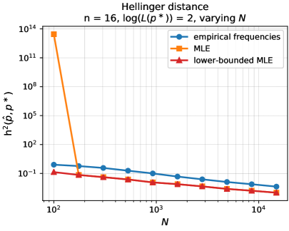
Refer to caption
Figure 6: Instability for small sample sizes in the Hellinger distance for varying N𝑁N and log(L(p))=2𝐿superscript𝑝2\log(L(p^{\ast}))=2

Acknowledgments

PR was supported in part by NSF awards IIS-1838071, DMS-1712596 and DMS-TRIPODS-1740751; ONR grant N00014-17- 1-2147 and grant 2018-182642 from the Chan Zuckerberg Initiative DAF. ER was supported in part by an NSF MSPRF DMS-1703821. We thank the anonymous reviewers for their constructive comments.

References

  • [1] R. Agrawal, U. Roy, and C. Uhler. Covariance matrix estimation under total positivity for portfolio selection. preprint arXiv:1909.04222, 2019.
  • [2] F. Bartolucci and A. Forcina. A likelihood ratio test for mtp_2𝑚𝑡𝑝_2mtp\_2 within binary variables. The Annals of Statistics, 28(4):1206–1218, 2000.
  • [3] D. Bates, S. Kornblith, A. Noack, M. Bouchet-Valat, M. K. Borregaard, J. M. White, A. Arslan, D. Kleinschmidt, G. Lynch, S. Lendle, P. K. Mogensen, I. Dunning, J. B. S. Calderón, D. Aluthge, pdeffebach, P. Bastide, J. Quinn, C. DuBois, B. Setzler, B. Born, R. Herikstad, M. Grechkin, L. Hein, J. TagBot, J. Adenbaum, H. Q. Ngo, D. Lin, and C. Caine. Juliastats/glm.jl: v1.3.9, Apr. 2020.
  • [4] M. Besançon, D. Anthoff, A. Arslan, S. Byrne, D. Lin, T. Papamarkou, and J. Pearson. Distributions.jl: Definition and modeling of probability distributions in the juliastats ecosystem. arXiv e-prints, page arXiv:1907.08611, Jul 2019.
  • [5] J. Bezanson, A. Edelman, S. Karpinski, and V. B. Shah. Julia: A fresh approach to numerical computing. SIAM review, 59(1):65–98, 2017.
  • [6] L. Birgé and P. Massart. Rates of convergence for minimum contrast estimators. Probability Theory and Related Fields, 97(1-2):113–150, 1993.
  • [7] Y. Chen. A tutorial on kernel density estimation and recent advances. Biostatistics & Epidemiology, 1(1):161–187, 2017.
  • [8] A. Colangelo, M. Scarsini, and M. Shaked. Some notions of multivariate positive dependence. Insurance: Mathematics and Economics, 37(1):13–26, 2005.
  • [9] M. Cule, R. Samworth, and M. Stewart. Maximum likelihood estimation of a multi-dimensional log-concave density. Journal of the Royal Statistical Society, Series B, 72:545–607, 2010.
  • [10] A. Domahidi, E. Chu, and S. Boyd. ECOS: An SOCP solver for embedded systems. In European Control Conference (ECC), pages 3071–3076, 2013.
  • [11] L. Dümbgen and K. Rufibach. Maximum likelihood estimation of a log-concave density and its distribution function: Basic properties and uniform consistency. Bernoulli, 15:40–68, 2009.
  • [12] B. Fang, A. Guntuboyina, and B. Sen. Multivariate extensions of isotonic regression and total variation denoising via entire monotonicity and Hardy-Krause variation. arXiv preprint arXiv:1903.01395, 2019.
  • [13] J. Felsenstein. Maximum-likelihood estimation of evolutionary trees from continuous characters. American Journal of Human Genetics, 25(471-492), 1973.
  • [14] C. Fortuin, P. Kasteleyn, and J. Ginibre. Correlation inequalities on some partially ordered sets. Communications in Mathematical Physics, 22(2):89–103, 1971.
  • [15] U. Grenander. On the theory of mortality measurement II. Skandinavisk Aktuarietidskrift, 39:125–153, 1956.
  • [16] P. Groeneboom and G. Jongbloed. Nonparametric Estimation under Shape Constraints. Cambridge University Press, Cambridge, 2014.
  • [17] P. Groeneboom, G. Jongbloed, and J. A. Wellner. Estimation of a convex function: Characterizations and asymptotic theory. Annals of Statistics, 29:1653–1698, 2001.
  • [18] A. J. Hoffman. On simple linear programming problems. In Proceedings of Symposia in Pure Mathematics, volume 7, pages 317–327, 1963.
  • [19] J. Hütter, C. Mao, P. Rigollet, and E. Robeva. Estimation of monge matrices. arXiv preprint arXiv:1904.03136, 2019.
  • [20] A. J. Izenman. Review papers: Recent developments in nonparametric density estimation. Journal of the American Statistical Association, 86(413):205–224, 1991.
  • [21] A. Juditsky, P. Rigollet, and A. B. Tsybakov. Learning by mirror averaging. The Annals of Statistics, 36(5):2183–2206, 2008.
  • [22] S. Karlin. Total positivity, volume 1. Stanford University Press, 1968.
  • [23] S. Karlin and J. McGregor. Coincidence probabilities. Pacific Journal of Mathematics, 9(4):1141–1164, 1959.
  • [24] S. Karlin and Y. Rinott. Classes of orderings of measures and related correlation inequalities. i. multivariate totally positive distributions. Journal of Multivariate Analysis, 10(4):467–498, 1980.
  • [25] S. Karlin and Y. Rinott. Total positivity properties of absolute value multinormal variables with applications to confidence interval estimates and related probabilistic inequalities. Annals of Statistics, 9:1035–1049, 1981.
  • [26] S. Karlin and Y. Rinott. M-matrices as covariance matrices of multinormal distributions. Linear Algebra and its Applications, 52:419–438, 1983.
  • [27] S. Lauritzen, C. Uhler, and P. Zwiernik. Maximum likelihood estimation in gaussian models under total positivity. arXiv:1702.04031, 2017.
  • [28] J. Lebowitz. Bounds on the correlations and analyticity properties of ferromagnetic ising spin system. Commun. math. Phys, 28(313-321), 1972.
  • [29] J. D. Lee, Y. Sun, and M. A. Saunders. Proximal Newton-type methods for minimizing composite functions. SIAM Journal on Optimization, 24(3):1420–1443, 2014.
  • [30] D. Lin, J. M. White, S. Byrne, D. Bates, A. Noack, J. Pearson, A. Arslan, K. Squire, D. Anthoff, T. Papamarkou, M. Besançon, J. Drugowitsch, M. Schauer, and other contributors. JuliaStats/Distributions.jl: a Julia package for probability distributions and associated functions, 2019.
  • [31] C. Mao, J. Weed, and P. Rigollet. Minimax rates and efficient algorithms for noisy sorting. Proceedings of the 28th International Conference on Algorithmic Learning Theory, 2018.
  • [32] P. Massart. Concentration inequalities and model selection: Ecole d’Eté de Probabilités de Saint-Flour XXXIII - 2003. Number no. 1896 in Ecole d’Eté de Probabilités de Saint-Flour. Springer-Verlag, 2007.
  • [33] A. Nemirovski. Topics in non-parametric statistics. Ecole d’Eté de Probabilités de Saint-Flour, 28:85, 2000.
  • [34] B. O’Donoghue, E. Chu, N. Parikh, and S. Boyd. Conic optimization via operator splitting and homogeneous self-dual embedding. Journal of Optimization Theory and Applications, 169(3):1042–1068, June 2016.
  • [35] B. O’Donoghue, E. Chu, N. Parikh, and S. Boyd. SCS: Splitting conic solver, version 2.0.2. https://github.com/cvxgrp/scs, Nov. 2017.
  • [36] W. Polonik. The silhouette, concentration functions and ML-density estimation under order restrictions. Annals of Statistics, 26:1857–1877, 1998.
  • [37] M. Queyranne, F. Spieksma, and F. Tardella. A general class of greedily solvable linear programs. Mathematics of Operations Research, 23(4):892–908, 1998.
  • [38] E. Robeva, B. Sturmfels, N. Tran, and C. Uhler. Maximum likelihood estimation for totally positive log-concave densities. arXiv preprint arXiv:1806.10120, 2018.
  • [39] E. Robeva, B. Sturmfels, and C. Uhler. Geometry of log-concave density estimation. arXiv:1704.01910, 2017.
  • [40] R. J. Samworth. Recent progress in log-concave density estimation. Statist. Sci., 33(4):493–509, 11 2018.
  • [41] D. W. Scott. Multivariate Density Estimation: Theory, Practice, and Visualization. John Wiley & Sons, 2015.
  • [42] A. Seregin and J. A. Wellner. Nonparametric estimation of convex-transformed densities. Annals of Statistics, 38:3751–3781, 2010.
  • [43] B. W. Silverman. Density Estimation for Statistics and Data Analysis. Routledge, 2018.
  • [44] M. Slawski and M. Hein. Estimation of positive definite M-matrices and structure learning for attractive Gaussian Markov random field. Linear Algebra and its Applications, 473:145–179, 2015.
  • [45] G. Strang. Computational science and engineering, volume 791. Wellesley-Cambridge Press Wellesley, 2007.
  • [46] A. B. Tsybakov. Introduction to Nonparametric Estimation. Springer Series in Statistics. Springer, 2009.
  • [47] R. Vershynin. High-dimensional probability: An introduction with applications in data science, volume 47. Cambridge University Press, 2018.
  • [48] G. Walther. Detecting the presence of mixing with multiscale maximum likelihood. Journal of the American Statistical Association, 97:508–513, 2002.
  • [49] L. Wasserman. Topological data analysis. Annual Review of Statistics and Its Application, 5:501–532, 2016.