$\Lambda_{c}^{+}$ fragmentation functions from pQCD approach and the Suzuki model

Abstract

Through data analysis, we present new sets of nonperturbative fragmentation functions (FFs) for $\Lambda_{c}^{+}$ baryon both at leading and next-to-leading order (NLO) and, for the first time, at next-to-next-to-leading order (NNLO) in the minimal subtraction factorization scheme with five massless quarks. The FFs are determined by fitting all available data of inclusive single $\Lambda_{c}^{+}$ baryon production in $e^{+}e^{-}$ annihilation taken by the OPAL Collaboration at CERN LEP1 and Belle Collaboration at KEKB. We also estimate the uncertainties in the $\Lambda_{c}^{+}$ FFs as well as in the corresponding observables. In a completely different approach based on the Suzuki model, we will theoretically calculate the $\Lambda_{c}^{+}$ FF from charm quark and present our result at leading order perturbative QCD framework. A comparison confirms a good consistency between both approaches. We will also apply the $\Lambda_{c}^{+}$ FFs to make theoretical predictions for the energy distribution of $\Lambda_{c}^{+}$ produced through the top quark decay, to be measured at the CERN LHC.

I Introduction

Study of heavy hadrons properties provides a possibility for better understanding the quark-gluon interaction dynamics in the QCD framework. In this regards and due to ongoing experiments there are particular interests in hadron productions at the CERN LHC and the BNL Relativistic Heavy Ion Collider (RHIC). In this work, we study the production mechanism of heavy baryons through the fragmentation process. In a general expression, the fragmentation mechanism describes the hadronization process where a parton carrying large transverse momentum decays to form a jet containing the expected hadron Braaten:1993rw . The hadronization processes are described by the fragmentation functions (FFs) which refer to the probability densities of hadron productions from initial partons and make the nonperturbative aspects of hadroproduction processes. These functions along with the parton distribution functions (PDFs) Salajegheh:2018hfs construct nonperturbative inputs for the calculation of hadroproduction cross sections. In this work, we focus on the FFs of $\Lambda_{c}^{+}$ baryon through two different approaches. In the first approach which is usually called as the phenomenological approach, a specific form including some free parameters is proposed for the desired FF so that all these free parameters are extracted through experimental data analysis, see, for example, Refs. Kniehl:2012ti ; Binnewies:1998vm ; Kniehl:2008zza ; Salajegheh:2019srg ; Nejad:2015fdh ; Soleymaninia:2017xhc ; Salajegheh:2019ach ; Salajegheh:2019nea ; Soleymaninia:2018uiv ; Soleymaninia:2019sjo ; Mohamaditabar:2018ffo ; Anderle:2015lqa ; Bertone:2017tyb . In an alternative scheme based on the theoretical models, the heavy hadron FFs might be computed by the virtue of perturbative QCD with limited phenomenological parameters, see, for example, Refs. GomshiNobary:1994eq ; MoosaviNejad:2017rvi ; MoosaviNejad:2019 ; Nejad:2013vsa ; MoosaviNejad:2018ece ; MohammadMoosaviNejad:2018pyp ; MoosaviNejad:2016qdx ; Nejad:2014iba where the heavy hadron FFs are computed by use of the Suzuki model Suzuki:1977km . This elaborate model is related to the perturbative QCD framework where all convenient Feynman diagrams at each order of perturbative QCD are considered for the parton level of hadronization process. In this approach, the nonperturbative aspect of hadronization is emerged in the bound state wave function. Detailed description is presented in Section III.
Independent of approach used to extract the FFs, when these functions are computed at the initial scale of fragmentation they can be evolved to higher scales using the timelike Dokshitzer-Gribov-Lipatov-Altarelli-Parisi (DGLAP) evaluation equations DGLAP .
In this paper, we first use the phenomenological approach to obtain a set of gluon, charm- and bottom-quark FFs into the $\Lambda_{c}^{+}$ baryon through a global QCD fit to all available $e^{+}e^{-}$ single inclusive annihilation (SIA) data measured by OPAL Collaboration Alexander:1996wy ; Ackerstaff:1997ki at the CERN LEP1 and very recent data from Belle Collaboration Niiyama:2017wpp . In Ref. Kniehl:2006mw , the $\Lambda_{c}^{+}$ FFs were determined both at leading and next-to-leading order in the minimal subtraction factorization scheme ($\overline{MS}$) by fitting the fractional energy spectra of $\Lambda_{c}^{+}$ baryon measured by the OPAL in the $e^{+}e^{-}$ annihilation on the Z-boson resonance. In their work, authors have applied the zero-mass variable-flavor-number scheme (ZM-VFNS) or, in a short expression, the massless scheme, where heavy quarks are treated as massless partons as well. Recently, KKSS20 Collaboration has updated their previous analysis Kniehl:2006mw combining the data for $e^{+}e^{-}$ annihilation from OPAL and the recent one from Belle, see Ref. Kniehl:2020szu . Their strategy for constructing the $\Lambda_{c}^{+}$-FFs is the same as their previous work for D-meson Kneesch:2007ey . Their work is restricted to the NLO accuracy and they have not also evaluated the uncertainties for FFs and corresponding observables.
In the present work, we focus on the hadronization of gluon, charm- and bottom-quarks into the $\Lambda_{c}^{+}$ using the massless scheme and provide the first QCD analysis of $(g,c,b)\to\Lambda_{c}^{+}$ FFs at next-to-next-to-leading order (NNLO). Meanwhile, we go beyond Refs. Kniehl:2006mw ; Kniehl:2020szu and perform a full-fledged error estimation for the parton FFs as well as the resulting differential cross sections. In order to evaluate the error estimations we apply the well-known Hessian approach Pumplin:2000vx . Note that, our analysis is restricted to only three data sets from single inclusive annihilation process due to two reasons: firstly, we are not aware of any other such data from electron-positron annihilation, and secondly, due to the lack of other theoretical partonic cross sections for the production of partons at NNLO accuracy. Although, among all processes producing baryons, the $e^{+}e^{-}$ annihilation process provides the cleanest environment to calculate the FFs, being devoid of nonperturbative effects beyond fragmentation itself.
In the following and in a theoretical approach independent of data analysis, we compute the initial scale fragmentation function of charm quark to split into the S-wave $\Lambda_{c}^{+}$ baryon at lowest-order of perturbative QCD. For this approach, we employ the elaborate Suzuki model which contains most of kinematical and dynamical aspects of hadroproduction process. Finally, we shall compare the initial scale FF of $c\to\Lambda_{c}^{+}$ determined in both approaches. Our comparison shows a good consistency between both results.

In the Standard Model (SM) of particle physics, the top quark has very short life time so does not have enough time to form a bound state, then before it decays hadronization takes place. At the lowest order of perturbative QCD and at the parton level, the decay mode $t\to bW^{+}$ followed by $b\to X+$Jets is governed. Here, X refers to the detected hadrons in the final state. Thus, at the CERN LHC a proposed channel to indirect search for the top quark properties is to study the energy spectrum of produced hadrons through top decays. In this work, as an example of possible applications of extracted FFs, we make the theoretical predictions for the energy distributions of $\Lambda_{c}^{+}$ baryons in top quark decays at LO, NLO and NNLO. This prediction will be compared with the one obtained through using the fit parameters reported in Ref. Kniehl:2020szu . This comparison does also shows a good consistency between our analysis and the one performed in Ref. Kniehl:2020szu .

The outline of this paper is as follows: In Section II, we explain the theoretical framework of hadron production in $e^{+}e^{-}$ annihilation in the massless scheme and introduce our parametrization of the $c/b\to\Lambda_{c}^{+}$ FF at the initial scale. We will also describe the minimization method in our analysis and the approach used for determination of error estimation. All applied experimental data will be describe in this section and our LO, NLO and NNLO results will be presented and compared with the data fitted to. In Section III, through the perturbative QCD approach we provide a general discussion of the fragmentation process for the S-wave heavy baryon and determine the fragmentation distribution of c-quark to fragment into $\Lambda_{c}^{+}$ baryon at lowest-order of perturbative QCD. In Section. IV, predictions for the normalized-energy distributions of $\Lambda_{c}^{+}$ baryon produced from top decay are presented. Our conclusions are listed in Section V.

II Phenomenological approach for determination of $\Lambda_{c}^{+}$ FFs and their uncertainties

As was mentioned, one of the most common approach to calculate the unpolarized nonperturbative FFs is the phenomenological approach based on the data analysis. In order to present the theoretical predictions for the observables involving cross section of identified hadrons in the final state, considering different hierarchical features is vital which is mentioned in this section. In this regard, we first review the QCD framework including the standard factorization theorem for differential cross section in a hadronization process of single inclusive electron-positron annihilation. We shall also introduce the OPAL and Belle experimental data as the only data sets for $\Lambda_{c}^{+}$ production in SIA process. Finally, we indicate our theoretical formalisms for determination of $\Lambda_{c}^{+}$ FFs and describe our strategy to determine the uncertainties of FFs as well as corresponding theoretical cross sections.

II.1 QCD framework for $\Lambda_{c}^{+}$ baryon FFs

Our analysis depends on the normalized differential cross section $1/\sigma_{tot}\times d\sigma/dx_{\Lambda}$ of the annihilation process

$$e^{+}e^{-}\rightarrow(\gamma^{*},Z)\rightarrow\Lambda_{c}^{+}+X,$$ (1)

where, $X$ refers to the unobserved hadrons in the final state and $\Lambda_{c}^{+}$ is the identified hadron. As usual, the scaling variable $x_{\Lambda}$ is defined as $x_{\Lambda}=2p_{\Lambda}\cdot q/q^{2}$ where, $p_{\Lambda}$ and $q$ refer to the four-momentum of detected baryon and intermediate gauge boson, respectively, so that $s=q^{2}$ is the collision energy. In the center of mass (CM) frame, the scaling variable is simplified as $x_{\Lambda}=2E_{\Lambda}/\sqrt{s}$ where $E_{\Lambda}$ shows the energy of detected baryon.

The key implement to divide the perturbative and nonperturbative parts of the $e^{+}e^{-}$ annihilation process (1) is the factorization theorem in the QCD-improved parton model Collins:1998rz . According to this theorem, the differential cross section of process (1) is written as the convolution of differential partonic cross sections $d\sigma_{i}(e^{+}e^{-}\to i+X)/dx_{i}$, with the $\Lambda_{c}^{+}$-FFs which is denoted by $D_{i}^{\Lambda_{c}^{+}}$. Here, $i=g,u,\bar{u},\ldots,b,\bar{b}$ runs over the active partons so that the number of active flavors is dependent on the energy scale. In the ZM-VFNS (or zero-mass scheme) where all light and heavy quarks are considered as massless partons, the differential cross section normalized to the total one is written as Collins:1998rz

$$\frac{1}{\sigma_{tot}} \frac{d\sigma}{dx_{\Lambda}}(e^{+}e^{-}\rightarrow\Lambda_{c}^{+}+X)$$

$$=\sum_{i}\int^{1}_{x_{\Lambda}}\frac{dx_{i}}{x_{i}}\frac{1}{\sigma_{tot}}\frac{d\sigma_{i}}{dx_{i}}(x_{i},\mu_{R},\mu_{F})D^{\Lambda_{c}^{+}}_{i}(\frac{x_{\Lambda}}{x_{i}},\mu_{F}).$$ (2)

In the CM frame, the scaling variable $x_{i}$ is also defined as $x_{i}=2E_{i}/\sqrt{s}$ which refers to the energy of produced parton $i$ in units of the beam energy. In the relation above, the scales $\mu_{F}$ and $\mu_{R}$ are the factorization and renormalization scales, respectively. Normally, they are arbitrary quantities which appear in each order of perturbation but in order to omit the ambiguous logarithmic terms $\ln(s/\mu_{F}^{2})$ in the partonic cross sections, they are chosen to be $\mu_{F}=\mu_{R}=\sqrt{s}$.
The experimental data included in our analysis are normalized to the total hadronic cross section for the $e^{+}e^{-}$ annihilation. This cross section reads

$$\sigma_{tot} =\frac{4\pi\alpha^{2}(s)}{s}(\sum^{n_{f}}_{i}\tilde{e}^{2}_{i}(s))$$ (3)

$$\times(1+\alpha_{s}K^{(1)}_{QCD}+\alpha_{s}^{2}K^{(2)}_{QCD}+\cdots).$$

Here, $\alpha_{s}$ and $\alpha$ are the strong-coupling and fine-structure constants, respectively, and $\tilde{e}_{i}$ is the effective electroweak charge of quark $i$. The QCD perturbative coefficients $K^{(i)}_{QCD}$ are currently known up to NNLO accuracy Gorishnii:1990vf so that $K_{\rm QCD}^{(1)}=3C_{F}/(4\pi)$, where $C_{F}=4/3$, and $K_{\rm QCD}^{(2)}\approx 1.411$ Chetyrkin:1979bj .
In Eq. (II.1), the nonperturbative part of the process (1) related to the transition $i\to\Lambda_{c}^{+}$ is described by the $D_{i}^{\Lambda_{c}^{+}}(z,\mu_{F})$-FF, where the fragmentation parameter $z=x_{\Lambda}/x_{i}$ indicates the energy fraction passed on from parton $i$ to the $\Lambda_{c}^{+}$ baryon, i.e., $z=E_{\Lambda}/E_{i}$. Since the FFs depend on the factorization scale $\mu_{F}$, they are evaluated to the various scales of energies by the DGLAP evolution equations, i.e.

$$\mu^{2}\frac{dD_{i}^{\Lambda}}{d\mu^{2}}(x_{\Lambda},\mu)=\sum_{j}\int^{1}_{x_{\Lambda}}\frac{dx_{i}}{x_{i}}P_{ij}(\frac{x_{\Lambda}}{x_{i}},\alpha_{s}(\mu))D_{j}^{\Lambda}(x_{i},\mu),$$ (4)

where, $P_{ij}$ are the splitting functions which have been computed up to NNLO accuracy Mitov:2006ic ; Moch:2007tx ; Almasy:2011eq .

II.2 Theoretical formalism

According to the phenomenological approach, in order to extract the nonperturbative FFs, the $z$-distributions of $i\rightarrow\Lambda_{c}^{+}$ FFs at the starting scale $\mu_{0}$ are parametrized from the beginning and the free parameters are constrained from the SIA experimental data. Note that, the selection criterion for the best parametrization form is to score a minimum $\chi^{2}_{\tt global}$ value as small as possible with a set of fit parameters as minimal as possible. The $\chi^{2}_{\tt global}$ function is defined in our previous works in more details Soleymaninia:2017xhc ; Salajegheh:2019ach . Following Ref. Kniehl:2020szu , we parametrize the $z$-dependence of $c\to\Lambda_{c}^{+}$ and $b\to\Lambda_{c}^{+}$ FFs at the starting scale as suggested by Bowler Bowler:1981sb while the FFs of light flavors are assumed to be zero at the starting scale. Moreover, since the data set included in our analysis is limited to the SIA process we can not constrain the gluon FF at the initial scale, thus its corresponding FF is also set equal to zero at the initial scale, i.e.,

$$D^{\Lambda_{c}^{+}}_{i}(z,\mu_{0}^{2})=0,\leavevmode\nobreak\ \leavevmode\nobreak\ for\leavevmode\nobreak\ i=u,\bar{u},d,\bar{d},s,\bar{s},g.$$ (5)

The FFs of gluon and light flavors will be generated to higher energy scales via the DGLAP evaluation equations. As was mentioned, for the $c\rightarrow\Lambda_{c}^{+}$ and $b\rightarrow\Lambda_{c}^{+}$ fragmentation the following Bowler parametrization Bowler:1981sb is considered:

$$D^{\Lambda_{c}^{+}}_{c}(z,\mu_{0}^{2})=N_{c}(1-z)^{a_{c}}z^{-(1+b_{c}^{2})}e^{-b_{c}^{2}/z}$$

$$D^{\Lambda_{c}^{+}}_{b}(z,\mu_{0}^{2})=N_{b}(1-z)^{a_{b}}z^{-(1+b_{b}^{2})}e^{-b_{b}^{2}/z},$$ (6)

which includes six free parameters: $N_{c},a_{c}$, $b_{c},N_{b},a_{a}$ and $b_{b}$. It is found that the Bowler parametrization enables one to do excellent fits at each order of perturbation, i.e. LO, NLO and NNLO. Here, the initial scale is set as $\mu_{0}=4.301$ GeV which is a little grater than the bottom mass threshold $m_{b}=4.3$ GeV.
Consequently, we have six free parameters which should be extracted from the best QCD fit on the experimental data. The optimal values of fit parameters for the charm and bottom FFs are reported in Table 1 at each order of perturbation.

Table 1: The optimal values for the input parameters of the $c\to\Lambda_{c}^{+}$ and $b\to\Lambda_{c}^{+}$ FFs at the initial scale $\mu_{0}^{2}=18.5$ GeV² determined by QCD analysis of the experimental data listed in Table 2.

Parameter		Best values
	LO	NLO	NNLO
$N_{c}$	$1928924455.183$	$15210639.353$	$2720317.971$
$a_{c}$	$2.343$	$2.373$	$2.458$
$b_{c}$	$4.343$	$3.814$	$3.597$
$N_{b}$	$578.441$	$323.094$	$318.980$
$a_{b}$	$9.302$	$9.138$	$9.321$
$b_{b}$	$1.554$	$1.477$	$1.464$

Technically, it should be mentioned that for the evolution of $D^{\Lambda^{+}_{c}}_{i}(z,\mu^{2})$-FFs as well as for the calculation of SIA cross sections up to NNLO accuracy we employed the publicly available APFEL package Bertone:2013vaa and the free parameters of FFs are determined by minimizing the $\chi^{2}_{\tt global}$ function using the CERN program MINUIT James:1975dr . Furthermore, to estimate the uncertainties of $D^{\Lambda^{+}_{c}}_{i}(z,\mu^{2})$-FFs the data uncertainties are propagated to the extracted QCD fit parameters using the asymmetric Hessian method (or Hessian methodology), as is outlined in Martin:2009iq ; Stump:2001gu . More details can be found in our previous analysis Salajegheh:2019ach .

II.3 Experimental data and fit results

In our analysis, we applied two data sets measured by OPAL Collaboration at the CERN LEP1 Collider Alexander:1996wy . In fact, for the SIA process (1) two different mechanisms contribute with similar rates; direct production through $Z\rightarrow c\bar{c}$ decay followed by the fragmentation $c/\bar{c}\to\Lambda_{c}^{+}$ and the decay $Z\rightarrow b\bar{b}$ (b-tagged events) followed by the fragmentation of $b$ (or $\bar{b}$) into the bottom-flavored hadron $H_{b}$, i.e., $b/\bar{b}\to H_{b}$, where finally the weak decay of $H_{b}$ into the $\Lambda_{c}^{+}$-baryon occurs; $H_{b}\to\Lambda_{c}^{+}+X$. Consequently, the energy spectrum of $\Lambda_{c}^{+}$-baryon originating from the decay of $H_{b}$-hadron is much softer than that due to primary charm production, as is expected. In order to separate charmed hadron production through the decay process $Z\rightarrow c\bar{c}$ from the decay $Z\rightarrow b\bar{b}$, the OPAL Collaboration investigated the apparent decay length distributions as well as the energy spectra of charmed hadrons. As is expected, the decay lengths of $H_{b}$ hadrons into $\Lambda_{c}^{+}$ baryon are always longer than those from prompt production. Note that, the OPAL Collaboration has presented $x_{\Lambda}$-distributions for their $\Lambda_{c}^{+}$ sample and for the b-tagged ($Z\to b\bar{b}$) subsamples. In addition to the OPAL data which includes only 4 points with rather large uncertainties we have also included a very recent data set measured by Belle Collaboration Niiyama:2017wpp at $\sqrt{s}=10.52$ GeV. This new data set is much more precise and contains more points. Belle data dose not have contributions from B-meson decays so that the contribution of $b\to\Lambda_{c}$ is not needed to be taken in the calculation of cross sections. However, the FFs from charm and bottom quarks are coupled through the DGLAP evolution equation. Following Ref. Kniehl:2020szu , we fix the $b\to\Lambda_{c}$ FF using the values of $N_{b},a_{b}$ and $b_{b}$ extracted from the OPAL fit. Therefore, the values of $N_{c},a_{c}$ and $b_{c}$ are yielded from the fit to the Belle data. Here, we describe a technical point over the reconstruction of old OPAL experimental data. OPAL data sets have been displayed in the form $(1/N_{\tt had})dN/dx_{\Lambda}$ where $N$ refers to the number of charmed-flavor hadron candidates which are reconstructed through appropriate decay chains. Therefore, in order to convert these data into the convenient cross section $(1/\sigma_{\tt tot})d\sigma/dx_{\Lambda}$, it is needed to divide them by the corresponding branching fractions of decays for the reconstruction of charmed-flavored baryons. In Refs. Alexander:1996wy ; Ackerstaff:1997ki , for the required branching fraction the following value is applied:

$$Br(\Lambda_{c}^{+}\rightarrow pK^{-}\pi^{+})=(4.4\pm 0.6)\%.$$ (7)

Since, in our analysis we are including both the old OPAL data and more recent Belle data which are based on the observation of decay $\Lambda_{c}^{+}\rightarrow pK^{-}\pi^{+}$, then we have to use the same branching ratio to reconstruct both data sets. Since, the Belle analysis has applied the newest branching ratio as $Br(\Lambda_{c}^{+}\rightarrow pK^{-}\pi^{+})=(6.635)\%$ Patrignani:2016xqp , we therefore rescale the old OPAL data by the factor $0.044/0.0635=0.6929$.

Another point about the Belle data is that we have to exclude data at small values of the scaling variable $z\leq 0.5$, since the theory is not reliable in this range without taking resummation of soft-gluon logarithms into account. Note that, no kinematical cut is taken over the OPAL data.

Dataset	Observable	$\sqrt{s}$[GeV]	$N_{n}^{data}$	$\chi^{2}$ (LO)	$\chi^{2}$ (NLO)	$\chi^{2}$ (NNLO)
Belle	Inclusive	10.52	35	41.419	42.843	55.413
OPAL	Inclusive	91.2	4	1.971	0.444	0.299
	$b$-tagged	91.2	4	4.520	4.524	4.539
TOTAL:			43	47.948	47.812	60.251
($\chi^{2}$/ d.o.f)				1.296	1.292	1.628

Table 2: The individual $\chi^{2}$ values for inclusive and $b$-tagged cross sections obtained at LO, NLO and NNLO. The total $\chi^{2}$ and $\chi^{2}/d.o.f$ fit for $\Lambda_{c}^{+}$ are also shown.

In Table. 2, the characteristics of available experimental data including the number of data points $N_{n}^{data}$ are presented. We have also listed the individual values of $\chi^{2}$ for inclusive and $b$-tagged data sets at LO, NLO and NNLO accuracies. Considering the number of degrees of freedom (d.o.f), i.e., $43-6=37$, we have also presented the total $\chi^{2}$ divided by the number of d.o.f at LO ($\chi^{2}/d.o.f=1.296$), NLO ($\chi^{2}/d.o.f=1.292$) and NNLO ($\chi^{2}/d.o.f=1.628$). As is seen, these values are around 1 for individual data sets so this confirms a well-satisfying fit in all three accuracies. From Table. 2, it is seen that a reduction in $\chi^{2}/d.o.f$ occurs when passing from LO to NLO accuracy. This behavior is not valid when NNLO corrections are considered. This is due to the fact that, the Belle cross sections have been measured at small scale of energy ($\sqrt{s}=10.52$ GeV) where the corrections for the finite mass of hadron and partons are more effective than the higher order corrections. Remember that we have used the ZM-VFN scheme where the hadron and parton masses are set to zero from the beginning. Nevertheless, the NNLO corrections lead to a reduction in the uncertainties bands of FFs and corresponding observables. See Figs. 1-4.

In order to show the consistency and goodness between the theoretical prediction and the experimental data used in the fits, in Fig. 1 we have plotted the inclusive differential cross section, as reported by Belle, and in Fig. 2 we have plotted the b-tagged and total differential cross sections normalized to the total one evaluated with our respective $\Lambda_{c}^{+}$ FFs. Both are compared with the Belle and OPAL data sets fitted to. In these figures, the uncertainty bands are also plotted using the Hessian approach. Through this approach, we just considered the uncertainties due to the experimental data sets so that we ignored additional sources of uncertainties. As is seen the quality of fit is improved when passing to higher order corrections. From Fig. 2, it is seen that our theoretical descriptions at LO, NLO and NNLO for both b-tagged and total differential cross sections are in good mutual agreement. The consistency seems to be better for the normalized total differential cross section (shown in lower panel) in comparison with the b-tagged one because our theoretical predictions do not go across one of the b-tagged data points located at $x_{\Lambda}=0.8$. This is why higher values of individual $\chi^{2}$ occur for b-tagged, see Table. 2.

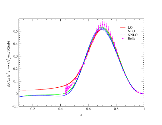
Figure 1: Using our extracted $\Lambda_{c}^{+}$-FFs, the theoretical predictions for inclusive differential cross sections at LO (red solid line), NLO (green dashed line) and NNLO (blue dot-dashed line) in $\sqrt{s}=10.52$ GeV are compared with Belle experimental data points fitted to. Corresponding uncertainty bands stem from $\Lambda_{c}^{+}$ FFs are shown as well.

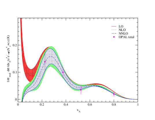
Figure 2: Same as Fig. 1 but for OPAL experimental data at $\sqrt{s}=M_{Z}$.

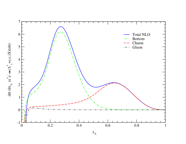
Figure 3: The NLO contribution of $c\rightarrow\Lambda_{c}^{+}$ (red dashed line), $b\rightarrow\Lambda_{c}^{+}$ (green dot-dashed line) and $g\rightarrow\Lambda_{c}^{+}$ (black dashed-dot-dot line) in inclusive differential cross section at $\sqrt{s}=M_{Z}$. The total contribution of all partons (blue solid line) is also plotted.

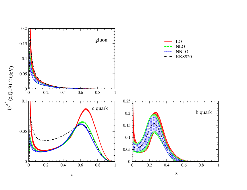
Figure 4: The gluon-, charm- and bottom-FFs with their uncertainties obtained at LO (red solid lines), NLO (green dashed lines) and NNLO (blue dot-dashed lines) QCD analyses of $\Lambda_{c}^{+}$ baryon productions at $\mu=M_{Z}$. The NLO KKSS20 results Kniehl:2020szu (black dashed-dashed-dot curves) are also plotted.

In Fig. 2, it is also seen that the behavior of theoretical predictions in small values of $x_{\Lambda}$ for the lowest order accuracy is completely different with the ones at NLO and NNLO. Obviously, in one hand, the theoretical cross section at LO goes to infinity when $x_{\Lambda}\to 0$ and, on the other hand, the LO uncertainty band is anomalously wider than the NLO and NNLO ones in all ranges of $x_{\Lambda}$. Therefore, the LO results are not reliable so that higher order radiative corrections need to be considered.
In order to show the fragmentation contribution of gluon, charm- and bottom-quark to the production of $\Lambda_{c}^{+}$, in Fig. 3 we have plotted these contributions at the scale $\sqrt{s}=M_{Z}$. The total differential cross section at NLO is also shown which is obtained by the sum of all contributions. As is expected, the contribution of gluon fragmentation is very tiny and it increases at small range of $x_{\Lambda}$. At large $x_{\Lambda}$, the contribution of charm quark (red dashed line) is governed while at small region the contribution of bottom quark (green dot-dashed line) is governed.

In Fig. 4, the $z$-distributions of $\Lambda_{c}^{+}$-FFs are plotted at $\mu_{F}=M_{Z}$; the energy scale of OPAL data sets fitted to. For this purpose, we plotted the $(c,b,g)\to D_{\Lambda^{+}_{c}}$ FFs at LO (solid lines), NLO (dashed lines) and NNLO (dot-dashed lines). From this plot, it is seen that the fragmentation of charm-quark is peaked at large-$z$ whereas the bottom fragmentation has its maximum at small-$z$. This behavior is due to the fact that the fragmentation process $b\to\Lambda_{c}^{+}$ contains two-step mechanism. In Fig. 4, the uncertainty bands of $\Lambda_{c}^{+}$-FFs are also presented which are needed to visually quantify the remaining error of analysis. Since, the Belle date does not include the contributions from the $b\to\Lambda_{c}$ fragmentation in the calculation of cross sections, then the uncertainties of $b$-quark FF are considerably much wider than the charm and gluon ones in each order of perturbation. Moreover, the error bands of all flavors decrease by increasing the order of perturbation. In Fig. 4, the NLO KKSS20 results Kniehl:2020szu (dashed-dashed-dot curves) are also plotted. As is seen, our result for gluon fragmentation is in good agreement with the one presented by KKSS20. In comparison to the KKSS20’s results, there is a considerable difference between the KKSS20 charm FF and ours in the range $z<0.5$. However, the behavior of our bottom-FF is the same as the KKSS20 one in the whole range of $z$. Unlike our procedure in which we set the same scale for the c- and b-quark FFs, the KKSS20 collaboration has selected different initial scales so that in their work the starting scales for the charm- and bottom-FFs were taken to be $\mu_{0}=m_{c}=1.5$ GeV and $\mu_{0}=m_{b}=5$ GeV, respectively.

III Theoretical approach for $\Lambda_{c}^{+}$ baryon FF

As was mentioned in the Introduction, apart from the phenomenological approaches to determine the nonperturbative FFs there are also some theoretical models to compute them. In fact, it was fortunately understood that for heavy hadron productions these functions can be analytically calculated by virtue of perturbative QCD (pQCD) including limited phenomenological parameters Ma:1997yq ; Braaten:1993mp . The first theoretical effort to illustrate the procedure of heavy hadron production was established by Bjorken Bjorken:1977md , so that in the following, Suzuki Suzuki:1977km , Ji and Amiri Amiri:1986zv have applied the pQCD approach considering elaborate models to describe the hadronization process. Since the Suzuki model includes most of the kinematical and dynamical aspects of hadroproduction process it gives us a detailed insight on the hadronization process. Especially, this model is much suitable to consider the spin effects of produced hadron or fragmenting parton which is absent in the phenomenological approach, see for example Nejad:2015far . It does also enable us to describe the gluon hadronization process which is not well determined in the phenomenological approach, see Refs. Nejad:2015oca ; Delpasand:2020mqv ; Delpasand:2019xpk .

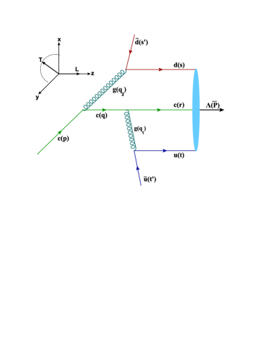
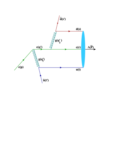
Figure 5: The lowest-order Feynman diagrams contributing to the fragmentation of charm-quark into the $\Lambda_{c}^{+}(ucd)$ baryon.

In this section, using the Suzuki model we focus on the fragmentation of $\Lambda_{c}^{+}$-baryon from charm quark for which the respective Feynman diagrams at leading order in $\alpha_{s}$ are shown in Fig. 5. According to this model, the FF for the production of an S-wave heavy bound state $M$ in hadronization of an initial heavy quark $Q$ might be put in the following general relation Suzuki:1977km

$$D_{Q}^{M}(z,\mu_{0}) =$$ (10)

$$\frac{1}{1+2s_{Q}}\sum_{\begin{array}[]{c}spin\\ color\end{array}}\int|T_{M}|^{2}\delta^{3}(\sum_{f}\bm{p}_{f}-\bm{p}_{Q})\Pi_{f}d^{3}\bm{p}_{f},$$

where, $\bm{p}_{Q}$ and $\bm{p}_{f}$ are the momenta of the fragmenting quark and the final particles, respectively. The fragmentation parameter $z$ is as the one introduced in the phenomenological approach (section II.A), i.e., $z=E_{M}/E_{Q}$ which takes the values as $0\leq z\leq 1$. Furthermore, $\mu_{0}$ stands for the initial fragmentation scale which is in order of fragmenting heavy quark mass and $s_{Q}$ refers to the fragmenting quark spin. In the above relation, the quantity $T_{M}$ is the probability amplitude for the hadron production. In the Suzuki model, this amplitude at large momentum transfer is expressed in terms of the hard scattering amplitude $T_{H}$ and the process-independent distribution amplitude $\Phi_{M}$ describing the nonperturbative dynamics of bound state. In fact, the long-distance amplitude $\Phi_{M}$ is, in essence, the probability amplitude for constituent quarks to be evolved into the final bound state. Therefore, the amplitude $T_{M}$ is expressed as Amiri:1986zv ; Brodsky:1985cr

$$T_{M}=\int\Pi_{j}dx_{j}\delta(1-\sum_{j}x_{j})T_{H}\Phi_{M}(x_{j},Q^{2}),$$ (11)

where, $x_{j}=E_{j}/E_{M}$ is the energy fraction carried by the constituent quark $j$ of heavy bound state $M$.
Considering the general definition (10) and the Feynman diagrams shown in Fig. 5, for the production of S-wave $\Lambda_{c}^{+}$-baryon from the initial charm quark, the FF of $c\to\Lambda_{c}^{+}$ is written as

$$D_{c}^{\Lambda_{c}^{+}}(z,\mu_{0}) =\frac{1}{2}\sum_{s,c}\int|T_{\Lambda}|^{2}$$

$$\times\delta^{3}(\bar{\bm{P}}+\bm{s}^{\prime}+\bm{t}^{\prime}-\bm{p})d^{3}\bar{\bm{P}}d^{3}\bm{s}^{\prime}d^{3}\bm{t}^{\prime},$$ (12)

where, four-momenta are as labeled in Fig. 5, and

$$T_{\Lambda} (p,\bar{P},s^{\prime},t^{\prime})$$

$$=\int_{0}^{1}dx_{1}dx_{2}dx_{3}\delta(1-x_{1}-x_{2}-x_{3})$$

$$\hskip 28.45274pt\times T_{H}(p,\bar{P},s^{\prime},t^{\prime},x_{i})\Phi_{B}(x_{i},Q^{2}).$$ (13)

The advantage of above scheme is to absorb the soft behavior of produced bound state into the hard scattering amplitude $T_{H}$ Brodsky:1985cr . Ignoring the details, the distribution amplitude $\Phi_{B}$ is related to the valence wave function $\Psi$ Brodsky:1985cr . Following Ref. Suzuki:1977km , we adopt the infinite momentum frame where the distribution amplitude $\Phi_{B}$, with neglecting the Fermi motion of constituents, reads MoosaviNejad:2016scq ; MoosaviNejad:2018ukp

$$\Phi_{B}=f_{B}\delta(x_{i}-\frac{m_{i}}{M}),$$ (14)

where, the baryon decay constant $f_{B}$ is related to the nonrelativistic S-wave function $\Psi(0)$ at the origin as $f_{B}=\sqrt{12/M}|\Psi(0)|$.

In Eq. (III), the short-distance amplitude $T_{H}$ can be calculated perturbatively considering the Feynman diagrams shown in Fig. 5, where a charm-quark creates a heavy baryon $\Lambda_{c}^{+}$ along with two light antiquarks $\bar{u}$ and $\bar{d}$. In the old-fashioned noncovariant perturbation theory, the hard scattering amplitude $T_{H}$ may be expressed as follows to keep the initial heavy quark on mass shell all the time Suzuki:1985up

$$T_{H}=\frac{g_{s}^{4}m_{\Lambda}m_{c}m_{d}m_{u}C_{F}}{2\sqrt{2p_{0}\bar{P}_{0}s^{\prime}_{0}t^{\prime}_{0}}}\times\frac{\sum_{i=1}^{2}\Gamma_{i}}{D_{0}},$$ (15)

where, $D_{0}=\bar{P}_{0}+s^{\prime}_{0}+t^{\prime}_{0}-p_{0}$ is the energy denominator, $C_{F}$ is the usual color factor and $\Gamma_{i}$ represents an appropriate combination of the propagators and the spinorial parts of the amplitude. In the above equation, the amplitudes $\Gamma_{i}$ stand for each Feynman diagrams in Fig. 5.
Substituting all expressions in Eq. (III) and carrying out the necessary integrations, we find

$$D_{c}^{\Lambda_{c}^{+}}(z,\mu_{0}) =N\int\frac{d^{3}\bm{s}^{\prime}d^{3}\bm{t}^{\prime}}{t_{0}^{\prime}s_{0}^{\prime}}\int\frac{\frac{1}{2}\sum_{i,j=1}^{2}\Gamma_{i}\bar{\Gamma}_{j}}{\bar{P}_{0}p_{0}D_{0}^{2}}$$

$$\times\delta^{3}(\bar{\bm{P}}+\bm{s}^{\prime}+\bm{t}^{\prime}-\bm{p})d^{3}\bar{\bm{P}},$$ (16)

where, $N\propto(f_{B}m_{\Lambda}m_{c}m_{d}m_{u}g_{s}^{4}C_{F})^{2}$.
In the above relation, using the well-known completeness relations $\sum_{spin}u(p)\bar{u}(p)=(\displaystyle{\not}{p}+m)$ and $\sum_{spin}v(q)\bar{v}(q)=(\displaystyle{\not}{q}-m)$ in the unpolarized Dirac string, one has

$$\sum_{i,j=1}^{2}\Gamma_{i}\bar{\Gamma}_{j} =$$ (17)

$$G_{1}^{2}Tr[(\not{s}^{\prime}-m_{d})\gamma^{\mu}(\displaystyle{\not}{s}+m_{d})\gamma^{\nu}T_{\mu\sigma\rho\nu}(\not{t^{\prime}}-m_{u})\gamma^{\sigma}(\not{t}+m_{u})\gamma^{\rho}]+$$

$$G_{2}^{2}Tr[(\not{t^{\prime}}-m_{u})\gamma^{\sigma}(\not{t}+m_{u})\gamma^{\rho}T_{\sigma\mu\nu\rho}(\not{s^{\prime}}-m_{d})\gamma^{\mu}({\not}{s}+m_{d})\gamma^{\nu}]$$

$$+2G_{1}G_{2}\times$$

$$Tr[(\not{s^{\prime}}-m_{d})\gamma^{\mu}({\not}{s}+m_{d})\gamma^{\nu}T_{\mu\sigma\nu\rho}(\not{t^{\prime}}-m_{u})\gamma^{\sigma}(\not{t}+m_{u})\gamma^{\rho}],$$

where,

$$T_{\mu\sigma\rho\nu} = (\displaystyle{\not}{p}+m_{c})\gamma_{\mu}(\displaystyle{\not}{q}+m_{c})\gamma_{\sigma}(\displaystyle{\not}{r}+m_{c})\gamma_{\rho}(\displaystyle{\not}{q}+m_{c})\gamma_{\nu},$$

$$T_{\sigma\mu\nu\rho} = (\displaystyle{\not}{p}+m_{c})\gamma_{\sigma}(\not{q^{\prime}}+m_{c})\gamma_{\mu}(\displaystyle{\not}{r}+m_{c})\gamma_{\nu}(\not{q^{\prime}}+m_{c})\gamma_{\rho},$$

$$T_{\mu\sigma\nu\rho} = (\displaystyle{\not}{p}+m_{c})\gamma_{\mu}(\not{q^{\prime}}+m_{c})\gamma_{\sigma}(\displaystyle{\not}{r}+m_{c})\gamma_{\nu}(\not{q}+m_{c})\gamma_{\rho}.$$

In the above expressions, after using the Dirac algebra and the traditional trace technique the dot products of four-momenta will appear. To proceed we need to specify our kinematics to determine the relevant dot products. Considering the Feynman diagrams shown in Fig. 5, where by ignoring the Fermi motion of quark constituents the $\Lambda_{c}^{+}$ baryon is replaced by its collinear constituents, the relevant four-momenta are set as

$$p_{\mu}=[p_{0},\bm{p}_{T},p_{L}],\quad t_{\mu}^{\prime}=[t_{0}^{\prime},\bm{t^{\prime}}_{T},t_{L}^{\prime}],$$

$$s_{\mu}^{\prime}=[s_{0}^{\prime},\bm{s^{\prime}}_{T},s_{L}^{\prime}],\quad r_{\mu}=[r_{0},\bm{0},r_{L}],$$

$$t_{\mu}=[t_{0},\bm{0},t_{L}],\qquad s_{\mu}=[s_{0},\bm{0},s_{L}],$$

$$\bar{P}_{\mu}=[\bar{P}_{0},\bm{0},\bar{P}_{L}],$$ (19)

where, $\bar{P}_{L}=r_{L}+t_{L}+s_{L}$ and we also assumed that the produced baryon moves along the $\hat{z}$-axes (fragmentation axes). According to the definition of fragmentation parameter, i.e., $z=\bar{P}_{0}/p_{0}$, the baryon takes a fraction $z$ of the energy of initial heavy quark (each constituent a fraction of $x_{1}$, $x_{2}$ and $x_{3}$) and two antiquarks take the remaining $1-z$ (each one with a fraction of $x_{4}$ and $x_{5}$). Thus, the parton energies can be expressed in terms of the initial heavy quark energy $p_{0}$, as

$$\bar{P}_{0}=zp_{0},\quad s_{0}=x_{1}zp_{0},\quad r_{0}=x_{2}zp_{0},\quad t_{0}=x_{3}zp_{0},$$

$$s_{0}^{\prime}=x_{4}(1-z)p_{0},\quad t_{0}^{\prime}=x_{5}(1-z)p_{0},$$ (20)

where, the condition $x_{1}+x_{2}+x_{3}=1$ holds as well as $x_{4}+x_{5}=1$. Moreover, according to our assumption that baryon moves along the $\hat{z}$-axes, the transverse momentum of initial quark is carrying by two antiquarks so that in the infinite momentum frame we have $s^{\prime}_{T}=x_{4}p_{T}$ and $t^{\prime}_{T}=x_{5}p_{T}$. With the approximation (14), we are postulating that the contribution of each constituent from the baryon energy is proportional to its mass, namely, $x_{i}=m_{i}/M$ where $M=m_{u}+m_{d}+m_{c}$ . We also assume that $x_{4}=m_{d}/m^{\prime}$ and $x_{5}=m_{u}/m^{\prime}$ where $m^{\prime}=m_{d}+m_{u}$.

Regarding the kinematics introduced, the dot products of relevant four-momenta read

$$s^{\prime}\cdot t^{\prime} = s\cdot t=m_{u}m_{d},$$

$$s\cdot r = m_{c}m_{d}\quad,\quad t\cdot r=m_{c}m_{u},$$

$$p\cdot s^{\prime} = \frac{m_{d}}{2}\beta\quad,\quad p\cdot t^{\prime}=\frac{m_{u}}{2}\beta,$$

$$p\cdot s = \frac{m_{d}}{2}\eta\quad,\quad p\cdot r=\frac{m_{c}}{2}\eta,$$

$$p\cdot t = \frac{m_{u}}{2}\eta\quad,\quad s\cdot s^{\prime}=\frac{m_{d}^{2}}{2}\alpha,$$

$$t\cdot t^{\prime} = \frac{m_{u}^{2}}{2}\alpha\quad,\quad r\cdot t^{\prime}=\frac{m_{u}m_{c}}{2}\alpha,$$

$$r\cdot s^{\prime} = \frac{m_{d}m_{c}}{2}\alpha\quad,\quad s\cdot t^{\prime}=\frac{m_{d}m_{u}}{2}\alpha$$ (21)

where,

$$\eta = \frac{M}{z}+\frac{zm_{c}^{2}}{M}(1+\frac{p_{T}^{2}}{m_{c}^{2}}),$$ (22)

$$\alpha = \frac{zm^{\prime}}{M(1-z)}(1+\frac{p_{T}^{2}}{m^{\prime 2}})+\frac{(1-z)M}{zm^{\prime}},$$

$$\beta = \frac{m_{c}^{2}(1-z)}{m^{\prime}}(1+\frac{p_{T}^{2}}{m_{c}^{2}})+\frac{m^{\prime}}{1-z}(1+\frac{p_{T}^{2}}{m^{\prime 2}})-2\frac{p_{T}^{2}}{m^{\prime}}.$$

In Eq. (17), $G_{1}$ and $G_{2}$ are related to the denominator of propagators as

$$G_{1} = \frac{1}{m_{d}^{3}m_{u}^{2}(2+\alpha)^{2}(m_{d}(2+\alpha)-\eta-\beta)},$$

$$G_{2} = \frac{1}{m_{d}^{2}m_{u}^{3}(2+\alpha)^{2}(m_{u}(2+\alpha)-\eta-\beta)}.$$ (23)

For the phase space integrations in the relation (III), one has

$$\int\frac{d^{3}\bar{\bm{P}}\delta^{3}(\bar{\bm{P}}+\bm{t^{\prime}}+\bm{s^{\prime}}-\bm{p})}{\bar{P}_{0}p_{0}D_{0}^{2}}=\frac{z}{G^{2}(z)},$$ (24)

where, $G(z)=M^{2}-m_{c}^{2}-m_{u}^{2}-m_{d}^{2}-2t^{\prime}\cdot s^{\prime}+2p\cdot t^{\prime}+2p\cdot s^{\prime}=m^{\prime}(2m_{c}+\beta)$, so that for the remaining integrals, according to the Suzuki model and for simplicity, we replace the transverse momentum integrations by their average values, e.g.,

$$\int d^{3}\bm{t^{\prime}}\frac{f(z,t_{T}^{\prime 2})}{t_{0}^{\prime}}\approx m_{u}^{2}f(z,\left\langle t_{T}^{\prime 2}\right\rangle),$$ (25)

where, according our assumption one has $t_{T}^{\prime}=x_{5}p_{T}=(m_{u}/m^{\prime})p_{T}$.
Substituting all in Eq. (III), the hadronization process $c\to\Lambda_{c}^{+}$ is described by the following function

$$D_{c}^{\Lambda_{c}^{+}}(z,\mu_{0})= N\frac{z\times\sum_{i,j=1}^{2}\Gamma_{i}\bar{\Gamma}_{j}}{\left[2m_{c}+\beta(z)\right]^{2}}\Bigg{|}_{p_{T}^{2}\to\left\langle p_{T}^{2}\right\rangle},$$ (26)

where, $N\propto(f_{B}m_{\Lambda}m_{c}m_{d}^{2}m_{u}^{2}g_{s}^{4}C_{F})^{2}/m^{\prime 2}$ but it is determined via $\int_{0}^{1}D_{c}^{\Lambda_{c}^{+}}(z,\mu_{0})dz=1$ (normalization condition) Amiri:1986zv .
In the above relation, $\sum_{i,j=1}^{2}\Gamma_{i}\bar{\Gamma}_{j}$ is given in (17) which is simplified in terms of dot products of four-momenta after using the Dirac algebra. Due to the lengthy and cumbersome expression for this term we ignore to present analytical result and just show our numerical analysis. Note that, in the Suzuki model the fragmentation function depends on both the fragmentation parameter $z$ and the phenomenological parameter $\left\langle p_{T}^{2}\right\rangle$. Although, the $z$-dependence of FFs is not yet calculable at each desired scale, but once they are computed at the initial fragmentation scale $\mu_{0}$, their $\mu$ evolution is determined through the DGLAP equations  DGLAP . In the Suzuki model, the initial scale is the minimum value of the invariant mass of the fragmenting parton. Therefore, the FF presented in Eq. (26) should be regarded as a model for the $c\to\Lambda_{c}^{+}$ transition at the initial scale $\mu_{0}=m_{\Lambda}+m_{u}+m_{d}$.

For our numerical analysis, we adopt the input parameters as $m_{c}=1.43\leavevmode\nobreak\ \textrm{GeV},m_{d}=4.67\leavevmode\nobreak\ \textrm{MeV},m_{u}=2.16\leavevmode\nobreak\ \textrm{MeV},f_{B}=0.25\leavevmode\nobreak\ \textrm{GeV}$, and $\alpha_{s}(m_{c})=0.38$ Tanabashi:2018oca . The color factor $C_{F}$ is calculated using the simple color line counting rule so we applied $C_{F}=7/6$ for our purpose.

In Fig. 6, taking $\left\langle p_{T}^{2}\right\rangle=1$ GeV² our theoretical prediction for the $D_{c}^{\Lambda_{c}^{+}}$-FF at the starting scale $\mu_{0}$ is shown (dotted line). In Refs. GomshiNobary:1994eq ; MoosaviNejad:2016qdx , it is shown that the choice of $\left\langle p_{T}^{2}\right\rangle=1$ GeV² is an optimum value for this quantity so that any higher value of this parameter will produce the peak position even at lower-z regions. To check the validity of the Suzuki model, using the parameters presented in Table. 1 we have also plotted the $D_{c}^{\Lambda_{c}^{+}}(z,\mu_{0})$-FF at LO (dashed line), NLO (solid line) and NNLO (dot-dashed line). As is seen, there is a considerable consistency between both approaches. This allows one to rely on the Suzuki model to determine the heavy quark FFs. As was mentioned previously, the Suzuki model is much suitable to consider the spin effects of produced hadrons or fragmenting partons which is absent in the phenomenological approach. It does also enable us to describe the gluon hadronization process which is not well determined in the phenomenological approach. It also gives one a detailed insight on the hadronization process because includes most of the kinematical and dynamical aspects of hadroproduction process.

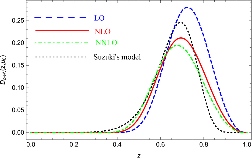
Figure 6: The $D_{c}^{\Lambda_{c}^{+}}(z,\mu_{0})$-FF at lowest-order in the Suzuki model (black dotted line) taking $\left\langle p_{T}^{2}\right\rangle=1$ GeV². This is compared with the ones extracted through the phenomenological approach at LO (blue dashed line), NLO (red solid line) and NNLO (green dot-dashed line). Here, we set $\mu_{0}=m_{\Lambda}+m_{u}+m_{d}$.

IV $\Lambda_{c}^{+}$ Baryon production by top quark decay

In this section, as a topical application of our baryon FFs, we study the inclusive single production of $\Lambda_{c}^{+}$ at the CERN LHC. Generally, the $\Lambda_{c}^{+}$ baryon may be produced directly or via the decay process of heavier particles, including the Higgs boson, the $Z$ boson, and the top quark. At the LHC, the study of energy distributions of observed hadrons through top quark decays might be considered as an indirect channel to search for the properties of top quarks. Since the top quark discovery by the $D0$ and CDF experiments at Fermilab Tevatron Group:2009ad , the full determination of its properties has not yet been performed so it has been one of the main aims in top physics theories.

In the Standard Model of particle physics, the top has a very short life time ($\tau_{t}\approx 0.5\times 10^{-24}$ s Chetyrkin:1999ju ) which is much shorter than the typical time to form the QCD bound states, i.e., $\tau_{\rm QCD}\approx 1/\Lambda_{\rm QCD}\approx 3\times 10^{-24}$ s, then the top quark decays rapidly before hadronization takes place. Related to the Cabibbo-Kobayashi-Maskawa (CKM) mixing matrix element for which $V_{tb}\approx 1$ Cabibbo:1963yz , top quarks almost exclusively decay to bottom quarks via $t\to bW^{+}$ so, in the following, produced bottom quarks hadronize by producing final jets. Therefore, a suggestion for a new channel to look for top properties at the LHC is to study the inclusive single $\Lambda_{c}^{+}$-baryon production through the following process

$$t\rightarrow bW^{+}(+g)\rightarrow\Lambda_{c}^{+}W^{+}+X,$$ (27)

where, $X$ collectively represents any other final-state particles. At the parton level, both the bottom quark and the gluon may hadronize into the $\Lambda_{c}^{+}$-baryon so that the gluon fragmentation contributes to the real radiations at NLO.
According to the factorization theorem of QCD-improved parton model jc , the partial width of the decay process (27) differential in the scaled $\Lambda_{c}^{+}$-baryon energy, $x_{\Lambda}$, is expressed as

$$\frac{d\Gamma}{dx_{\Lambda}}=\sum_{i=b,g}\int_{x_{i}^{min}}^{x_{i}^{max}}\frac{dx_{i}}{x_{i}}\,\frac{d\Gamma_{i}}{dx_{i}}(\mu_{R},\mu_{F})D_{i}^{\Lambda_{c}^{+}}\left(\frac{x_{\Lambda}}{x_{i}},\mu_{F}\right),$$ (28)

where the factorization and the renormalization scales, i.e., $\mu_{F}$ and $\mu_{R}$, are arbitrary but to avoid large logarithms appearing in the parton differential decay rates $d\Gamma_{i}/dx_{i}$, we set $\mu_{R}=\mu_{F}=m_{t}$, as usual. For simplicity, we shall work in the top-rest frame in which the scaling variables are defined as $x_{\Lambda}=E_{\Lambda}/E_{b}^{\mathrm{max}}$ and $x_{i}=E_{i}/E_{b}^{\mathrm{max}}$, where $E_{\Lambda}$ and $E_{i}$ stand for the energies of $\Lambda_{c}^{+}$ baryon and parton $i$, respectively. Here, $E_{b}^{\mathrm{max}}=m_{t}(1-\omega)/2$ is the maximum energy of the bottom quark in the process (27), where $\omega=(m_{W}/m_{t})^{2}$. At present, analytic expressions for the Wilson coefficient functions $d\Gamma_{i}/dx_{i}$ are only available at NLO accuracy which are computed in Refs. Nejad:2013fba ; Kniehl:2012mn . Using our extracted $(b,g)\to\Lambda_{c}^{+}$ FFs at LO and NLO, we make our predictions for the energy spectrum of $\Lambda_{c}^{+}$-baryon produced through the unpolarized top quark decay. However, a consistent analysis is presently restricted to NLO approximation, but we also employ the NNLO set of $D_{c}^{\Lambda_{c}^{+}}$-FF to probe the possible size of NNLO corrections.

Adopting the input parameters as $m_{t}=173$ GeV and $m_{W}=80.379$ GeV, in Fig. 7 we studied the energy distribution of $\Lambda_{c}^{+}$-baryon in unpolarized top decays at LO (dotted line), NLO (dashed line) and NNLO (solid line). As is seen, switching from the LO $\Lambda_{c}^{+}$-baryon FF set to the NLO one slightly smoothens the theoretical prediction, decreasing it in the peak region and the tail region thereunder. In Fig. 7, the results for $d\Gamma/dx_{\Lambda}$ are also compared to the evaluation with the KKSS20 $\Lambda_{c}^{+}$-baryon FF set Kniehl:2020szu . As is seen, there is a good consistency between both results. In comparison with the KKSS20 spectrum, the peak position of our results is shifted towards larger values of $x_{\Lambda}$.

At the LHC, the study of energy distribution of $\Lambda_{c}^{+}$-baryon may be also considered as a new window towards searches on new physics. Practically, for the energy distribution of produced hadrons any considerable deviation from the SM predictions can be assigned to the new physics. For example, it would be a signal for the existence of charged Higgs bosons produced from $t\to\Lambda_{c}^{+}H^{+}$ in the theories beyond the SM MoosaviNejad:2012ju ; MoosaviNejad:2019agw ; MoosaviNejad:2016aad ; MoosaviNejad:2016jpc ; MoosaviNejad:2011yp . Meanwhile, the study of $x_{\Lambda}$-distribution in the decay mode (27) will enable us to deepen our understanding of the nonperturbative aspects of baryon formation by hadronization. Moreover, through studying these distributions the $b/g\to\Lambda_{c}^{+}$ FFs can be also constrained event further.

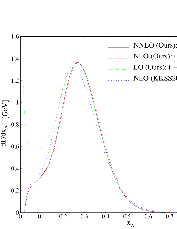
Figure 7: The LO (green dotted line), NLO (red dashed line) and NNLO (black solid line) predictions of $d\Gamma(t\to\Lambda_{c}^{+}+Jets)/dx_{\Lambda}$ evaluated with our $\Lambda_{c}^{+}$-baryon FF sets. For comparison, the evaluation with the NLO KKSS20 $\Lambda_{c}^{+}$-FF set Kniehl:2006mw is also included (blue dot-dashed line). Here, we set the scale as $\mu=m_{t}$.

V Summary and Conclusions

Through this work, we determined the nonperturbative unpolarized FFs for the charmed baryon $\Lambda_{c}^{+}$ in two various approaches; phenomenological analysis and theoretical approach based on the Suzuki model. Employing the theoretical model we computed the $\Lambda_{c}^{+}$-FF at lowest-order of perturbative QCD whereas using the phenomenological approach we determined the $\Lambda_{c}^{+}$-FFs both at LO, NLO and, for the first time, at NNLO accuracy in the ZM-VFN scheme by fitting to all available data of inclusive single $\Lambda_{c}^{+}$-baryon production in $e^{+}e^{-}$ annihilation from OPAL and Belle Collaborations Ackerstaff:1997ki ; Niiyama:2017wpp . A comparison between both approaches showed a good consistency between results. Note that, the theoretical framework provided by the ZM-VFN scheme is quite appropriate for our data analysis because the characteristic energy scales of annihilation process, i.e., $M_{Z}$, greatly exceeds the c- and b-quark masses, which could thus be neglected. For our data analysis, we adopted the same functional form for the parameterization of charm and bottom FFs with three free parameters, see Eqs. (II.2). From Fig. 2, it is seen that in the lowest-order approximation the behavior of theoretical cross section is not acceptable at low-$x_{\Lambda}$ region but it is reasonably improved when higher order radiative corrections are considered. Through the following aspects, our analysis on the $\Lambda_{c}^{+}$-baryon FFs improves a similar analysis in previous works Kniehl:2006mw ; Kniehl:2020szu . Firstly, we increased the precision of calculation to NNLO, however due to few numbers of experimental data for $\Lambda_{c}^{+}$-baryon production our results showed that the effect of this correction is not considerable. Secondly, we did an accurate estimation of the experimental uncertainties in the $\Lambda_{c}^{+}$-FFs using the Hessian approach. The uncertainties bands of FFs as well as corresponding observables show that the NNLO radiative corrections affect the error band and decrease them considerably. Meanwhile, we have compared, for the first time, the analytical result obtained for the $D_{c}^{\Lambda_{c}^{+}}(z,\mu_{0})$-FF through the Suzuki model with the one extracted via the phenomenological analysis. A good consistency between both approaches ensure the Suzuki model, see Fig. 6. This model is suitable to consider the spin effect of produced hadron or/and initial parton on the corresponding FFs, a subject absent in data analysis approach. On the other hand, as is well-known, the gluon FF’s play a significant role in hadroproduction but they are only feebly constrained by $e^{+}e^{-}$ data. But, through the Suzuki model it would be possible to determine them analytically, see Refs. MoosaviNejad:2019 ; Nejad:2014iba ; Nejad:2015far .
As a topical application of our obtained FFs, we used the LO, NLO and NNLO FFs to make our theoretical predictions for the scaled-energy distributions of $\Lambda_{c}^{+}$-baryon inclusively produced in unpolarized top decays. This channel is proposed for independent determination of $\Lambda_{c}^{+}$-baryon FFs which provides a unique chance to test their universality and DGLAP scaling violations; two important pillars of the QCD-improved parton model. Furthermore, this study provides a new window towards searches on new physics.
For theoretical approach, one can think of other possible improvements including the Fermi motion of constituents. This is done by considering the real aspects of the valence wave function of baryon Brodsky:1985cr ; MoosaviNejad:2020svj , etc. Related to the phenomenological approaches, improvements due to the inclusion of finite quark masses and the resummation of soft-gluon logarithms would be effective. These effects extend the validity of analysis towards small and large values of $x_{\Lambda}$, respectively. In this regards, the general-mass variable-flavor-number scheme (ZM-VFNS) Nejad:2016epx ; Abbaspour:2017pyp where the charm- and bottom-quark masses are preserved from the beginning provides a consistent and natural finite mass generalization of the ZM-VFNS on the basis of the $\overline{\mathrm{MS}}$ factorization scheme Collins:1998rz . The implementation of these improvements reaches beyond the scope of our present analysis and is left for future researches.

References

- (1) E. Braaten and T. C. Yuan, Phys. Rev. Lett. 71, 1673 (1993).
- (2) M. Salajegheh, S. M. Moosavi Nejad, M. Nejad, H. Khanpour and S. Atashbar Tehrani, Phys. Rev. C 97 (2018) no.5, 055201.
- (3) B. A. Kniehl, G. Kramer, I. Schienbein and H. Spiesberger, Eur. Phys. J. C 72, 2082 (2012).
- (4) J. Binnewies, B. A. Kniehl and G. Kramer, Phys. Rev. D 58, 034016 (1998).
- (5) B. A. Kniehl, G. Kramer, I. Schienbein and H. Spiesberger, Phys. Rev. D 77, 014011 (2008).
- (6) M. Salajegheh, S. M. Moosavi Nejad and M. Delpasand, Phys. Rev. D 100 (2019) no.11, 114031.
- (7) S. M. Moosavi Nejad, M. Soleymaninia and A. Maktoubian, Eur. Phys. J. A 52 (2016) no.10, 316.
- (8) M. Soleymaninia, H. Khanpour and S. M. Moosavi Nejad, Phys. Rev. D 97, no. 7, 074014 (2018).
- (9) M. Salajegheh, S. M. Moosavi Nejad, H. Khanpour, B. A. Kniehl and M. Soleymaninia, Phys. Rev. D 99 (2019) no.11, 114001
- (10) M. Salajegheh, S. M. Moosavi Nejad, M. Soleymaninia, H. Khanpour and S. Atashbar Tehrani, Eur. Phys. J. C 79 (2019) no.12, 999.
- (11) M. Soleymaninia, M. Goharipour and H. Khanpour, Phys. Rev. D 98, no. 7, 074002 (2018).
- (12) M. Soleymaninia, M. Goharipour and H. Khanpour, Phys. Rev. D 99, no. 3, 034024 (2019).
- (13) A. Mohamaditabar, F. Taghavi-Shahri, H. Khanpour and M. Soleymaninia, Eur. Phys. J. A 55 (2019) no.10, 185.
- (14) D. P. Anderle, F. Ringer and M. Stratmann, Phys. Rev. D 92 (2015) no.11, 114017.
- (15) V. Bertone et al. [NNPDF Collaboration], Eur. Phys. J. C 77 (2017) no.8, 516.
- (16) M. A. Gomshi Nobary, J. Phys. G 20 (1994) 65.
- (17) S. M. Moosavi Nejad, Phys. Rev. D 96 (2017) no.11, 114021.
- (18) Mahdi. Delpasand and S. Mohammad. Moosavi Nejad, Phys. Rev. D 99 (2019), 114028.
- (19) S. M. Moosavi Nejad and A. Armat, Eur. Phys. J. Plus 128 (2013) 121.
- (20) S. M. Moosavi Nejad and E. Tajik, Eur. Phys. J. A 54 (2018) no.10, 174.
- (21) S. Mohammad Moosavi Nejad and A. Armat, Eur. Phys. J. A 54 (2018) no.7, 118.
- (22) S. M. Moosavi Nejad and P. Sartipi Yarahmadi, Eur. Phys. J. A 52 (2016) no.10, 315.
- (23) S. M. Moosavi Nejad and D. Mahdi, Int. J. Mod. Phys. A 30 (2015) 1550179.
- (24) M. Suzuki, Phys. Lett. B 71 (1977) 139.
- (25) V. N. Gribov and L. N. Lipatov, Sov. J. Nucl. Phys. 15 (1972) 438 [Yad. Fiz. 15 (1972) 781]; G. Altarelli and G. Parisi, “Asymptotic Freedom in Parton Language,” Nucl. Phys. B 126 (1977) 298.
- (26) G. Alexander et al. [OPAL Collaboration], Z. Phys. C 72, 1 (1996).
- (27) K. Ackerstaff et al. [OPAL Collaboration], Eur. Phys. J. C 1, 439 (1998).
- (28) M. Niiyama et al. [Belle], Phys. Rev. D 97, no.7, 072005 (2018) doi:10.1103/PhysRevD.97.072005 [arXiv:1706.06791 [hep-ex]].
- (29) B. A. Kniehl and G. Kramer, Phys. Rev. D 74, 037502 (2006).
- (30) B. Kniehl, G. Kramer, I. Schienbein and H. Spiesberger, [arXiv:2004.04213 [hep-ph]].
- (31) T. Kneesch, B. Kniehl, G. Kramer and I. Schienbein, Nucl. Phys. B 799, 34-59 (2008) doi:10.1016/j.nuclphysb.2008.02.015 [arXiv:0712.0481 [hep-ph]].
- (32) J. Pumplin, D. R. Stump and W. K. Tung, Phys. Rev. D 65, 014011 (2001).
- (33) J. C. Collins, Phys. Rev. D 58, 094002 (1998).
- (34) S. G. Gorishnii, A. L. Kataev and S. A. Larin, Phys. Lett. B 259, 144 (1991).
- (35) K. G. Chetyrkin, A. L. Kataev and F. V. Tkachov, Phys. Lett. 85B, 277 (1979).
- (36) A. A. Almasy, S. Moch and A. Vogt, Nucl. Phys. B 854, 133 (2012).
- (37) S. Moch and A. Vogt, Phys. Lett. B 659, 290 (2008).
- (38) A. Mitov, S. Moch and A. Vogt, Phys. Lett. B 638, 61 (2006).
- (39) M. G. Bowler, Z. Phys. C 11, 169 (1981).
- (40) V. Bertone, S. Carrazza and J. Rojo, Comput. Phys. Commun. 185 (2014) 1647.
- (41) F. James and M. Roos, Comput. Phys. Commun. 10, 343 (1975).
- (42) A. D. Martin, W. J. Stirling, R. S. Thorne and G. Watt, Eur. Phys. J. C 63, 189 (2009).
- (43) D. Stump, J. Pumplin, R. Brock, D. Casey, J. Huston, J. Kalk, H. L. Lai and W. K. Tung, Phys. Rev. D 65, 014012 (2001).
- (44) C. Patrignani et al. [Particle Data Group], Chin. Phys. C 40 (2016) 100001.
- (45) J. P. Ma, Nucl. Phys. B 506, 329 (1997).
- (46) E. Braaten, K. m. Cheung and T. C. Yuan, Phys. Rev. D 48, 4230 (1993).
- (47) J. D. Bjorken, Phys. Rev. D 17 (1978) 171.
- (48) F. Amiri and C. -R. Ji, Phys. Lett. B 195 (1987) 593.
- (49) S. M. Moosavi Nejad and M. Delpasand, Int. J. Mod. Phys. A 30 (2015) no.32, 1550179.
- (50) S. M. Moosavi Nejad, Eur. Phys. J. Plus 130 (2015) no.7, 136.
- (51) M. Delpasand and S. M. Moosavi Nejad, Eur. Phys. J. A 56 (2020) no.2, 56.
- (52) M. Delpasand and S. M. Moosavi Nejad, Phys. Rev. D 99 (2019) no.11, 114028.
- (53) S. J. Brodsky and C. R. Ji, Phys. Rev. Lett. 55 (1985) 2257.
- (54) S. M. Moosavi Nejad, Eur. Phys. J. Plus 133 (2018) no.1, 25.
- (55) S. M. Moosavi Nejad, Eur. Phys. J. A 52 (2016) no.5, 127.
- (56) M. Suzuki, Phys. Rev. D 33 (1986) 676.
- (57) M. Tanabashi et al. [Particle Data Group], Phys. Rev. D 98, no. 3, 030001 (2018).
- (58) Tevatron Electroweak Working Group [CDF and D0 Collaborations], “Combination of CDF and D0 Results on the Mass of the Top Quark,” arXiv:0903.2503 [hep-ex].
- (59) K. G. Chetyrkin, R. Harlander, T. Seidensticker and M. Steinhauser, Phys. Rev. D 60, 114015 (1999).
- (60) N. Cabibbo, Phys. Rev. Lett. 10, 531 (1963); M. Kobayashi and T. Maskawa, Prog. Theor. Phys. 49, 652 (1973).
- (61) P. V. Pobylitsa, Phys. Rev. D 66, 094002 (2002).
- (62) S. M. M. Nejad, Phys. Rev. D 88 (2013) no.9, 094011;
- (63) B. A. Kniehl, G. Kramer and S. M. Moosavi Nejad, Nucl. Phys. B 862 (2012) 720;
- (64) S. M. Moosavi Nejad, Eur. Phys. J. C 72 (2012) 2224;
- (65) S. M. Moosavi Nejad, S. Abbaspour and R. Farashahian, Phys. Rev. D 99 (2019) no.9, 095012.
- (66) S. M. Moosavi Nejad and S. Abbaspour, Nucl. Phys. B 921 (2017) 86.
- (67) S. M. Moosavi Nejad and S. Abbaspour, JHEP 1703 (2017) 051.
- (68) S. M. Moosavi Nejad, Phys. Rev. D 85 (2012) 054010.
- (69) S. M. Moosavi Nejad, M. Roknabady and M. Delpasand, Nucl. Phys. B 956 (2020) 115036.
- (70) S. M. Moosavi Nejad and M. Balali, Eur. Phys. J. C 76 (2016) no.3, 173;
- (71) S. Abbaspour and S. M. Moosavi Nejad, Nucl. Phys. B 930 (2018) 270.