Search for Optically Dark Infrared Galaxies without Counterparts of Subaru Hyper Suprime-Cam in the AKARI North Ecliptic Pole Wide Survey Field

Abstract

We present the physical properties of AKARI sources without optical counterparts in optical images from the Hyper Suprime-Cam (HSC) on the Subaru telescope. Using the AKARI infrared (IR) source catalog and HSC optical catalog, we select 583 objects that do not have HSC counterparts in the AKARI North Ecliptic Pole (NEP) wide survey field ($\sim 5$ deg²). Because the HSC limiting magnitude is deep ($g_{\rm AB}$ $\sim 28.6$), these are good candidates for extremely red star-forming galaxies (SFGs) and/or active galactic nuclei (AGNs), possibly at high redshifts. We compile multi-wavelength data out to 500 $\micron$ and use it for Spectral Energy Distribution (SED) fitting with CIGALE to investigate the physical properties of AKARI galaxies without optical counterparts. We also compare their physical quantities with AKARI mid-IR selected galaxies with HSC counterparts. The estimated redshifts of AKARI objects without HSC counterparts range up to $z\sim 4$, significantly higher than that of AKARI objects with HSC counterparts. We find that: (i) 3.6 $-$ 4.5 $\micron$ color, (ii) AGN luminosity, (iii) stellar mass, (iv) star formation rate, and (v) $V$-band dust attenuation in the interstellar medium of AKARI objects without HSC counterparts are systematically larger than those of AKARI objects with counterparts. These results suggest that our sample includes luminous, heavily dust-obscured SFGs/AGNs at $z\sim 1-4$ that are missed by previous optical surveys, providing very interesting targets for the coming James Webb Space Telescope era.

1 Introduction

In the last two decades, it has become clear that dusty star-forming galaxies (SFGs) and active galactic nuclei (AGNs) play an important role in galaxy formation and evolution, and in co-evolution of galaxies and supermassive black holes (SMBHs) (see e.g., Goto et al., 2011; Casey et al., 2014; Hickox & Alexander, 2018; Chen et al., 2020, and references therein). They are particularly numerous in the high-z universe ($z>2$), the key epoch where the cosmic star formation rate (SFR) density and BH mass accretion rate density reach a maximum (e.g., Madau & Dickinson, 2014; Ueda et al., 2014; Aird et al., 2015). Blecha et al. (2018) conducted a smoothed-particle hydrodynamics and N-body simulation and reported that infrared (IR) color (3.4 and 4.6 $\micron$ color) correlates with AGN activity and nuclear obscuration in the framework of galaxy merger events–a redder system tends to have large AGN luminosity and hydrogen column density (see also Ricci et al., 2017; Ellison et al., 2019; Gao et al., 2020). Since dusty SFGs/AGNs often have redder color in the optical and near-IR (NIR), they could correspond to the maximum phase of SF/AGN activity. They would thus be the crucial population to understanding how the galaxies and their SMBHs co-evolve behind a large amount of dust (see also Hopkins et al., 2008; Narayanan et al., 2010).

Owing to the heavy extinction by so much dust, some high-z dusty AGNs/SFGs are optically faint or even optically “dark”. For example, dust-obscured galaxies (DOGs: Dey et al., 2008; Toba et al., 2015, 2017a; Noboriguchi et al., 2019) are characterized by a large mid-IR (MIR) – optical color; their optical flux density is about 10³ times fainter than that in the MIR band (see also Hwang et al., 2013a, b). They are considered as dusty SFGs or AGNs at $z\sim$1–2–the relative proportion of AGN/SF could increase with IR luminosity (Melbourne et al., 2012; Toba et al., 2017c, d; Riguccini et al., 2019). A more extreme DOG population, Hot DOGs (Eisenhardt et al., 2012; Wu et al., 2012) known as dusty AGNs at $z>2$ also tend to be optically-faint. Recently, some galaxies detected by Atacama Large Millimeter/submillimeter Array (ALMA) are recognized as invisible SFGs without optical/NIR counterparts (e.g., Franco et al., 2018; Yamaguchi et al., 2019; Williams et al., 2019; Wang et al., 2019).

AKARI, the first Japanese space satellite dedicated to IR astronomy (Murakami et al., 2007), has also a great potential to find such optically dark objects. In addition to all-sky surveys with MIR and far-IR (FIR) (Ishihara et al., 2010; Yamamura et al., 2010), AKARI performed deep and wide observations of the North Ecliptic Pole (NEP) over a total area of 5.4 deg² (Matsuhara et al., 2006). The AKARI NEP survey consists of two layers: NEP Wide (NEP-W; Lee et al., 2009; Kim et al., 2012) and NEP Deep (NEP-D; Wada et al., 2008; Takagi et al., 2010; Murata et al., 2013). AKARI NEP regions were observed with the Infrared Camera (IRC: Onaka et al., 2007), using its nine filters that continuously cover 2–25 $\micron$. They are called N2, N3, and N4 for the NIR bands, S7, S9W, and S11 for the shorter part of the MIR band (MIR-S), and L15, L18W, and L24 for the longer part of the MIR bands (MIR-L). The effective wavelength of the N2, N3, N4, S7, S9W, S11, L15, L18W, and L24 filters is about 2.4, 3.2, 4.1, 7.0, 9.0, 11.0, 15.0, 18.0, and 24.0 $\micron$, respectively. These continuous NIR-MIR filters that are critical to trace dust emission heated by AGNs and/or Polycyclic Aromatic Hydrocarbon (PAH) emission associated with SF activity. This makes AKARI/NEP data quite powerful to select AGNs and measure the SF activity up to $z\sim 2$ (e.g., Goto et al., 2011; Murata et al., 2014; Huang et al., 2017; Kim et al., 2019; Poliszczuk et al., 2019).

Recently, the AKARI NEP-W has been observed with Hyper Suprime-Cam (HSC; Miyazaki et al., 2018) (see also Furusawa et al., 2018; Kawanomoto et al., 2018; Komiyama et al., 2018) on the Subaru telescope (PI: T.Goto). Oi et al. (2020) reduced the data and used it to construct a five-band HSC catalog that contains 3,251,792 sources. The 5$\sigma$ detection limit for $g$-, $r$-, $i$-, $z$-, and $y$-band is about 28.6, 27.3, 26.7, 26.0, and 25.6 mag, respectively. Oi et al. (2020) cross-identified the HSC catalog with AKARI NEP-W catalog and found that $\sim$90,000 AKARI objects have HSC counterparts (hereafter AKARI–HSC objects) (see also S. J. Kim et al. 2020 in preparation). Using the AKARI–HSC objects, Goto et al. (2019) derived their IR luminosity function at $0.35<z<2.2$ and measured IR luminosity density as a function of redshift up to $z\sim 2$. Recently, Ho et al. (2020) calculated photometric redshifts ($z_{\rm photo}$) of AKARI–HSC objects, and demonstrated how the deep HSC data improve their accuracy. Wang et al. (2020) investigated the physical properties of AKARI–HSC objects based on spectral energy distribution (SED) fitting with CIGALE (Code Investigating GALaxy Emission: Burgarella et al., 2005; Noll et al., 2009; Boquien et al., 2019) (see also Chiang et al., 2019).

However, those works focused on AKARI sources that have optical (i.e., HSC) counterparts. In this work, we shed light on the remaining objects; AKARI sources without HSC counterparts in the AKARI NEP-W. Since the limiting magnitude of the HSC is deep, these sources are expected to be extremely red SFGs/AGNs at high redshifts. We carefully select the candidates and investigate their physical properties.

The structure of this paper is as follows. Section 2 describes the data set, sample selection of AKARI sources without HSC counterparts, and our SED modeling of them. In Section 3, we present the results of our SED fitting and the derived physical quantities. In Section 4, we compare the resultant physical properties with AKARI sources that have HSC counterparts (Wang et al., 2020). We summarize the results of the work in Section 5. Throughout this paper, the adopted cosmology is a flat universe with $H_{0}$ = 70.4 km s^-1 Mpc^-1, $\Omega_{M}$ = 0.272, and $\Omega_{\Lambda}$ = 0.728 (the Wilkinson Microwave Anisotropy Probe 7 cosmology: Komatsu et al., 2011), which are the same as those adopted in Wang et al. (2020). Unless otherwise noted, all magnitudes refer to the AB system and a Salpeter (1955) initial mass function (IMF) is assumed.

2 Data and Analysis

2.1 Data Set

To select AKARI sources without HSC counterparts securely and investigate their physical properties, we compile multi-wavelength data. AKARI NEP-W was observed by many facilities, and thus we have abundant dataset from ultraviolet (UV) to radio (see e.g., Kim et al., 2012; Oi et al., 2020, and references therein for a full description). We particularly utilized the following data sets in addition to the AKARI NEP-W catalog (Kim et al., 2012) and HSC catalog (Oi et al., 2020) that are summarized in Table 2.1. The area coverage of each dataset is summarized in Figure 1.

Table 1: Multi-wavelength Data Set.

Catalog	Band	5$\sigma$ detection limit (unit)
(Number of sources)
HSC	$g$	28.6 (AB mag)
(3,251,792)	$r$	27.3 (AB mag)
	$i$	26.7 (AB mag)
	$z$	26.0 (AB mag)
	$y$	25.6 (AB mag)
FLAMINGOS	$J$	21.6 (AB mag)
(295,383)	$H$	21.3 (AB mag)
$Spitzer$/IRAC	Ch1	6.45 ($\mu$Jy)
(380,858)	Ch2	3.95 ($\mu$Jy)
$AKARI$ NEP-W	N2	15.42 ($\mu$Jy)
(114,794)	N3	13.30 ($\mu$Jy)
	N4	13.55 ($\mu$Jy)
	S7	58.61 ($\mu$Jy)
	S9W	67.30 ($\mu$Jy)
	S11	93.76 ($\mu$Jy)
	L15	133.1 ($\mu$Jy)
	L18W	120.2 ($\mu$Jy)
	L24	274.4 ($\mu$Jy)
$Herschel$/SPIRE	250 $\micron$	9.0 (mJy)
(4,820)	350 $\micron$	7.5 (mJy)
	500 $\micron$	10.8 (mJy)

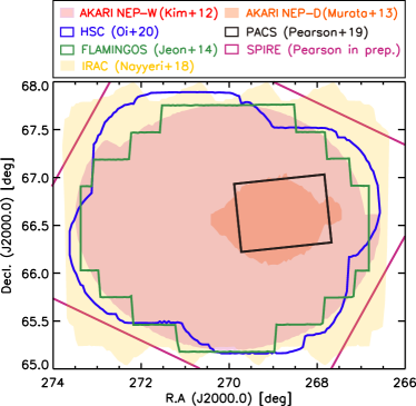
Figure 1: The footprint of each observation. Red, orange, and yellow shaded regions represent AKARI NEP-W (Kim et al., 2012), NEP-D (Murata et al., 2013), and IRAC/Spitzer (Nayyeri et al., 2018), respectively. Blue, green, black, and magenta line represent HSC/Subaru (Oi et al., 2020), FLAMINGOS/KPNO (Jeon et al., 2014), PACS/Herschel (Pearson et al., 2019), and SPIRE/Herschel (Pearson et al., 2017, C. Pearson in preparation), respectively.

We used NIR data provided by Jeon et al. (2014) who conducted a deep imaging with $J$- and $H$- bands taken by FLoridA Multi-object ImagingNear-ir Grism Observational Spectrometer (FLAMINGOS: Elston et al., 2006) on the Kitt Peak National Observatory (KPNO) 2.1 m telescope. This photometric catalog contains 295,383 sources with a 5$\sigma$ detection limit of 21.6 and 21.3 mag in the $J$- and $H$- bands, respectively.

For MIR data, we used a catalog of Nayyeri et al. (2018) who provided 3.6 $\micron$ (ch1) and 4.5 $\micron$ (ch2) data taken with Infrared Array Camera (IRAC: Fazio et al., 2004) on board the Spitzer Space Telescope (Werner et al., 2004). This photometric catalog contains 380,858 sources with a 5$\sigma$ detection limit of 6.45 and 3.95 $\mu$Jy in the 3.6 $\micron$ and 4.5 $\micron$ bands, respectively.

Regarding the FIR data, we utilized a recent catalog of 250, 350, and 500 $\micron$ (Pearson et al., 2017, C. Pearson in preparation). The data were taken with the Spectral and Photometric Imaging REceiver instrument (SPIRE: Griffin et al., 2010) on board the Herschel Space Observatory (Pilbratt et al., 2010). This SPIRE catalog contains 4,820 sources with a 5$\sigma$ detection limit of 9.0, 7.5, and 10.8 mJy at 250, 350, and 500 $\micron$, respectively (Barrufet et al., 2020). Note that AKARI NEP-D was observed by the Photoconductor Array Camera and Spectrometer (PACS: Poglitsch et al., 2010) at 100 and 160 $\micron$, and the catalog (including 1,384 and 630 sources detected by 100 and 160 $\micron$, respectively) is available (Pearson et al., 2019). But since the survey footprint is not so large ($\sim$0.7 deg², see Figure 1), we did not use the catalog in this work.

Eventually, we used 21 photometric data in total; $g$-, $r$-, $i$-, $z$-, $y$-, $J$-, and $H$-bands and 2.4 (N2), 3.2 (N3), 3.6 (ch1), 4.1 (N4), 4.5 (ch2), 7.0 (S7), 9.0 (S9W), 11.0 (S11), 15.0 (L15), 18.0 (L18W), 24.0 (L24), 250, 350, and 500 $\micron$, even though some of them are often upper limits (e.g., HSC five-bands).

2.2 Sample Selection

The procedure for sample selection is summarized in Figure 2.

Figure 2: Flow chart of the process to select AKARI sources without HSC counterparts.

The candidates of AKARI sources without HSC counterparts were drawn from the AKARI NEP-W sample in Kim et al. (2012) who provided 114,794 sources detected by the IRC. The 5$\sigma$ detection limit of N2, N3, N4, S7, S9W, S11, L15, L18W, and L24 is 15.42, 13.30, 13.55, 58.61, 67.30, 93.76, 133.1, 120.2, and 274.4 $\mu$Jy, respectively. Note that we selected candidates and obtained their multi-wavelength information by cross-matching with several catalogs in which coordinates in the AKARI NEP-W catalog were always referred. In this work, we attempt a cross-matching with a catalog by using a search radius that is much larger than a typical size of point spread function (PSF) for objects in the catalog. We then determined a search radius for cross-matching with a catalog as a 3$\sigma$ deviation from mean separation ($\Delta$R.A. and $\Delta$ Decl.) between AKARI NEP-W and that catalog, in the same manner as S. J. Kim et al. (2020, in preparation).

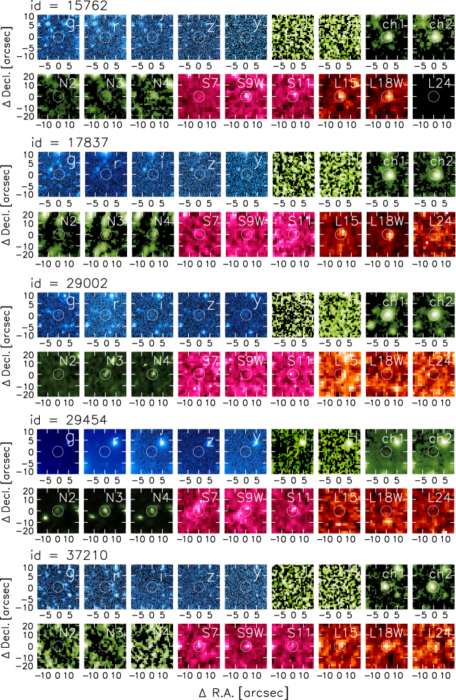
Figure 3: Examples of multi-wavelength images ($g$, $r$, $i$, $z$, $y$, $J$, $H$, ch1, ch2, N2, N3, N4, S7, S9W, S11, L15, L18W, and L24, from top left to bottom right) for AKARI sources without HSC counterparts. R.A. and Decl. are relative coordinate with respect to objects in the AKARI NEP-W catalog (Kim et al., 2012). White circles in the images also correspond to the coordinate of AKARI NEP-W catalog.

We first narrowed the sample to sources within the footprint observed by the HSC. This is because the HSC data do not cover quite the whole region of the AKARI NEP-W (see Figure 1), and hence some objects are just unobserved by the HSC. As a result, 109,734 objects were left out. We then removed 84,076 objects with nm $>$ 0 that were reported as having optical counterparts in Kim et al. (2012). They used optical catalogs provided by Hwang et al. (2007) and Jeon et al. (2010) in which the optical data were taken with MegaCam (Boulade et al., 2003) on the Canada-France-Hawaii Telescope (CFHT) and SNUCAM (Im et al., 2010) on the Maidanak observatory, respectively. Following that, we cross-identified the sample with the HSC catalog (Oi et al., 2020), which has a sensitivity roughly 5 times deeper than optical catalogs used in Kim et al. (2012), providing optically-faint AKARI sources. By adopting a search radius of 1.8″, 20,446 objects were cross-identified.

For $25,658-20,446=5,212$ AKARI sources, we removed contaminants. Because objects with magnitude brighter than $\sim$16 may be saturated in the MegaCam/SNUCAM/HSC images, they were removed from those catalogs before the cross-matching with AKARI NEP-W catalog. Therefore, some AKARI sources in our sample are expected to be bright stars/galaxies. In order to remove bright objects, we cross-identified the sample with Gaia DR2 (Gaia Collaboration, 2016, 2018) using a search radius of 1.6″. The Gaia DR2 catalog contains point sources with a $g$-band magnitude of 3–16. As a result, 534 bright objects were removed. We then extracted AKARI objects with 5$\sigma$ detections in at least one AKARI band and with clean photometry flag (i.e., flag_bandname_mag = 0). We also applied nfl = 0 to select objects unaffected by cosmic rays and/or multiplexer bleed trails in the NIR bands (see Section 2.2. in Kim et al., 2012), which yielded 3,734 objects.

Finally, we conducted a visual inspection to select reliable candidates in which we supplementarily used multi-wavelength images in $J$- and $H$-bands (FLAMINGOS) and ch1 and ch2 (IRAC) in addition to HSC and AKARI images. Consequently, 583 objects were selected as AKARI sources without HSC counterparts. Figure 3 shows examples of postage stamp images for our sample. Why were 3,734 – 583 = 3,151 objects removed? One reason is that the edges of the fields of view (FoV) of HSC may be degraded by artifacts. The AKARI NEP-W consists of 4-7 exposures by the HSC with a FoV of 1.5° in diameter through dithering observations. Therefore, objects around the edges of each exposure frame would be missed from the HSC catalog created by the HSC pipeline (Bosch et al., 2018) although they exist on the HSC image (see Oi et al., 2020, in details). Nevertheless, we should note that the visual inspection might be highly dependent on the classifier. The number of objects selected in this work may have an uncertainty. Hence, the population census results such as number counts and volume density of AKARI sources without HSC counterparts should be addressed in future work, and we focus on an overview of their physical properties in this work.

For those AKARI sources without HSC counterparts, we compiled a multi-wavelength dataset up to 500 $\micron$. We cross-identified the sample with FLAMINGOS, IRAC/Spitzer, and SPIRE/Herschel. In our sample, AKARI coordinates of each source were always used for the cross-matching. We employed 1.9″, 2.3″, and 6.6″as the search radius for cross-matching with FLAMINGOS, IRAC, and SPIRE, respectively. As stated, these search radii were determined to be 3$\sigma$ deviations from mean separation between AKARI objects without HSC counterparts and FLAMINGOS/IRAC/SPIRE catalogs. Accordingly, 70, 338, and 35 objects were cross-identified with FLAMINGOS, IRAC, and SPIRE, respectively. We found that 2/70, 4/338 and 2/35 AKARI objects have two candidate counterparts for FLAMINGOS, IRAC, and SPIRE, respectively. In this study, we chose the closest object as the counterpart for such cases. Among AKARI-bands, 425/583 (73%), 109/583 (19%), and 59/583 (10%) objects are detected in the NIR, MIR-S, and MIR-L, respectively, We note that 23 objects with L24 detection naturally satisfy DOG criterion, $(r-[24\,\micron])_{\rm AB}>7.5$ (Dey et al., 2008) owing to the limiting magnitude in the HSC $r$-band (26.7) and AKARI 24 $\micron$ (17.8), suggesting that our sample selection may preferentially select dusty galaxies (see also Section 4.2).

2.3 SED Fitting with CIGALE

Table 2: Parameter Ranges Used in the SED Fitting with CIGALE

Parameter	Value
Delayed SFH
$\tau_{\rm main}$ (Myr)	5000.0
$\tau_{\rm burst}$ (Myr)	20000
$f_{\rm burst}$	0.00, 0.01
age (Myr)	1000, 5000, 10000
SSP (Bruzual & Charlot, 2003)
IMF	Salpeter (1955)
Metallicity	0.02
Dust Attenuation (Charlot & Fall, 2000)
$\log$ ($A_{\rm V}^{\rm ISM}$)	-2, -1.7, -1.4, -1.1, -0.8, -0.5,
	-0.2 ,0.1, 0.4, 0.7, 1.0
slope_ISM	-0.9, -0.7, -0.5
slope_BC	-1.3, -1.0, -0.7
AGN Emission (Fritz et al., 2006)
$R_{\rm max}/R_{\rm min}$	60
$\tau_{\rm 9.7}$	0.3, 0.6
$\beta$	-0.5
$\gamma$	4.0
$\theta$	100.0
$\psi$	0.001, 60.100, 89.990
$f_{\rm AGN}$	0.1, 0.3, 0.5, 0.7, 0.9
Dust Emission (Draine et al., 2014)
$q_{\rm PAH}$	0.47, 1.77, 2.50, 5.26
$U_{\rm min}$	0.1, 1.0, 10, 50
$\alpha$	1.0, 1.5, 2.0, 2.5, 3.0
$\gamma$	0.01, 0.1, 1.0
Photometric Redshift
$z_{\rm photo}$	0.8, 1.0, 1.5, 2.0, 2.2, 2.4, 2.6, 2.8, 3.0,
	3.2, 3.4, 3.6, 3.8, 4.0, 4.2

We employed CIGALE to conduct detailed SED modeling in a self-consistent framework by considering the energy balance between the UV/optical and IR. This code enables us to handle many parameters, such as star formation history (SFH), single stellar population (SSP), attenuation law, AGN emission, dust emission, and radio synchrotron emission (see e.g., Boquien et al., 2014; Buat et al., 2014, 2015; Boquien et al., 2016; Ciesla et al., 2017; Lo Faro et al., 2017; Toba et al., 2019a; Burgarella et al., 2020; Toba et al., 2020a). Note that one of the purposes of this work is to compare the physical properties between AKARI sources with and without HSC counterparts. Wang et al. (2020) constructed AKARI L18W-selected sample with HSC counterparts, and also conducted the SED fitting with CIGALE to derive their physical properties. Therefore, to compare the resultant quantities under the same conditions, we chose the same models with the same parameter ranges as those Wang et al. (2020) adopted, except for AGN fraction in the AGN module and $\gamma$ in the dust module (see below). Parameter ranges used in the SED fitting are tabulated in Table 2.3.

We used a delayed SFH model, assuming a single starburst with an exponential decay (Ciesla et al., 2015, 2016), where we fixed e-folding times of the main stellar population ($\tau_{\rm main}$) and the late starburst population ($\tau_{\rm burst}$), while we parameterized the age of the main stellar population in the galaxy.

We utilized the stellar templates with solar metallicity provided from Bruzual & Charlot (2003) assuming the Salpeter (1955) IMF, and the standard default nebular emission model included in CIGALE (see Inoue, 2011).

Dust attenuation is modeled by using the Charlot & Fall (2000) with two different power-law attenuation curves that are parameterized by the power law slope of the attenuation in the interstellar medium (ISM) and birth clouds (BC). We also separately parameterized the $V$-band attenuation in the ISM ($A_{\rm V}^{\rm ISM}$).

For AGN emission, we used models provided by Fritz et al. (2006). In order to avoid a degeneracy of AGN templates in the same manner as in Ciesla et al. (2015) and Toba et al. (2019b), we fixed certain parameters that determine the number density distribution of the dust within the dust torus, i.e., ratio of the maximum to minimum radii of the torus ($R_{\rm max}/R_{\rm min}$), density profile along the radial and the polar distance coordinates parameterized by $\beta$ and $\gamma$ (see equation 3 in Fritz et al., 2006), and opening angle ($\theta$). We parameterized the optical depth at 9.7 $\micron$ ($\tau_{\rm 9.7}$) and $\psi$ parameter (an angle between equatorial axis and line of sight) that corresponds to our viewing angle of the torus. We further parameterized AGN fraction ($f_{\rm AGN}$), that is the contribution of AGN to the total IR luminosity (Ciesla et al., 2015). Note that we adopted a discrete interval for $f_{\rm AGN}$ compared with Wang et al. (2020) in which $f_{\rm AGN}$ is a key parameter to investigate the dependences of the fractional AGN contribution on IR luminosity and redshift. Our sample is basically detected in only several AKARI bands (and the remaining bands give upper-limits). This may often not be enough to constrain the $f_{\rm AGN}$ precisely. Hence we reduced the number of possible values of $f_{\rm AGN}$ considered.

Dust grain emission is modeled by Draine et al. (2014). The model is parameterized by the mass fraction of PAHs ($q_{\rm PAH}$), the minimum radiation field ($U_{\rm min}$), and the power-low slope of the radiation field distribution ($\alpha$) (see Equation 4 in Draine et al., 2014). We also parameterized the fraction illuminated with a variable radiation field ranging from $U_{\rm min}$ to $U_{\rm max}$ ($\gamma$) although Wang et al. (2020) fixed this at $\gamma$ = 1. We confirmed that parametrizing $\gamma$ gives a better fit to the FIR part of the spectra.

We also parameterized redshift to estimate photometric redshift ($z_{\rm photo}$), because by definition, our sample is optically too faint to obtain spectroscopic redshifts. Since the optically-dark galaxies tend to be located at $z>2$ (e.g., Franco et al., 2018; Yamaguchi et al., 2019; Williams et al., 2019; Wang et al., 2019), we optimized the range of $z_{\rm photo}$, which reduces the computing time. Aside from being an excellent SED-fitting tool, CIGALE is known to be a good estimator of $z_{\rm photo}$, since it utilizes a large number of models covering the whole SED including the MIR-FIR regime. For example, Małek et al. (2014) calculated $z_{\rm photo}$ for AKARI sources in the AKARI Deep Field South. They demonstrated that accuracy of the $z_{\rm photo}$ by using the normalized median absolute deviation defined as $\sigma_{\Delta z/(1+z_{\rm spec})}$ = 1.48 $\times$ median($|\Delta z|$/(1+$z_{\rm spec}$)) in the same manner as Ilbert et al. (2006). The resultant $\sigma_{\Delta z/(1+z_{\rm spec})}$ is 0.056, lower than what obtained by a software using mainly optical to NIR data (Ilbert et al., 2006) (see also Barrufet et al., 2020). On the other hand, the above AKARI sources have optical counterparts, i.e., they are moderately bright in the optical, and the sample is limited to the local universe ($z<0.25$). Since we constrain the optical SEDs based only on upper limits, we need to investigate the influence of our lack of optical data points on the accuracy of $z_{\rm photo}$ (see Section 4.6.1).

In order to ensure the reliability of the derived physical quantities including $z_{\rm photo}$, we extracted AKARI sources with 5$\sigma$ detections in at least 5 bands among the NIR-FIR, which yields 142/583 objects for SED fitting. If the signal-to-noise ratio (S/N) at a certain band is greater than 5.0, we used the photometry at that band. Otherwise, we put 10$\sigma$ upper limits that are drawn from each catalog (see Section 2.1).

3 Results

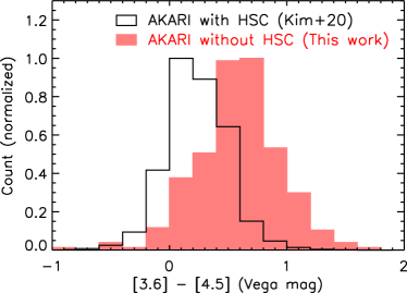
Figure 4: Normalized histogram of [3.6]-[4.5] color (in Vega magnitude) of AKARI sources with (black) and without (red) HSC counterparts.

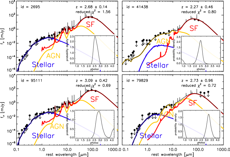
Figure 5: Examples of the SED fitting. The black points are photometric data. The contribution from the stellar, AGN, and SF components to the total SED are shown as blue, yellow, and red lines, respectively. The black solid line represents the resultant best-fit SED. The inserted panel shows the probability density distribution of redshift.

3.1 Comparison of IRAC Color

Before the SED fitting, we check the IRAC ch1 and ch2 color ([3.6] - [4.5] in Vega magnitudes) of our sample objects. Figure 4 shows IRAC color of 338 AKARI sources without HSC counterparts. We also plotted IRAC colors of AKARI sources with HSC counterparts where we used a multi-wavelength merged AKARI catalog provided by S. J. Kim et al. (2020, in preparation). We removed stars with stellarity parameter (that was measured from CFHT $r$-band or Maidanak $R$-band images) greater than 0.8 (see Kim et al., 2012). This left 42,264 objects for the comparison.

We find that [3.6]-[4.5] colors of AKARI sources without HSC counterparts (i.e., our sample) are systematically redder than those of AKARI sources with HSC counterparts. Blecha et al. (2018) reported that W1 (3.4 $\micron$) and W2 (4.6 $\micron$) color (almost same as IRAC ch1 and ch2 color) taken with the theWide-field Infrared Survey Explorer (WISE: Wright et al., 2010), is a good indicator of AGN activity and nuclear obscuration. The AGN luminosity and hydrogen column density peak during the galaxies’ coalescence, where W1–W2 color ranges from 0.8 –1.6 (see Figure 1 in Blecha et al. 2018). This suggests that a fraction of objects in our sample could correspond to luminous, obscured AGN phase.

3.2 Result of SED Fitting

Figure 5 shows examples of the SED fitting with CIGALE. We confirm that 91/142 ($\sim$64%) objects have reduced $\chi^{2}<3.0$ while 112/142 ($\sim$79%) objects have reduced $\chi^{2}<5.0$. This means that the data are moderately well fitted with the combination of the stellar, AGN, and SF components by CIGALE. We also confirm that the probability distribution function (PDF) of redshift does not have prominent secondary peaks for $\sim$90% of our sample in which a peak with 30% of the primary peak is considered as secondary peak (see top panels for objects without showing secondary peak and bottom panels for objects showing secondary peak in the PDF in Figure 5). The typical uncertainty of $z_{\rm photo}$ is about 20% (see also Section 4.6.1). Hereafter, we will focus on a subsample of 112 AKARI galaxies with reduced $\chi^{2}$ of their SED fitting smaller than 5.0 in the same manner as Toba et al. (2019b).

4 Discussions

Wang et al. (2020) constructed an 18 $\micron$ (L18W)-selected AKARI sample with HSC counterparts among which 443 objects have Herschel detections (SPIRE 250 $\micron$ or PACS 100 $\micron$) and spectroscopic redshifts (Shim et al., 2013; Oi et al., 2017; Kim et al., 2018; Shogaki et al., 2018). In order to derive their physical properties such as AGN luminosity and SFR, they performed SED fitting with CIGALE. What is the difference in the physical properties between AKARI objects with and without HSC counterparts? To ensure the relatability of the SED fitting, we will use 317 sources with reduced $\chi^{2}<5.0$ in sample provided by Wang et al. (2020) for the following discussion.

4.1 Stellar Mass

Figure 6: Histogram of the stellar mass of AKARI sources with (blue) and without (yellow) HSC counterparts. The red line represents stellar mass of our sample with L18W and SPIRE detections. Green line represents our sample with $\Delta$BIC $>$ 2.0 (see Section 4.6.2).

Figure 6 shows the stellar mass for AKARI sources with and without HSC counterparts. We find that the stellar mass of our sample galaxies is systematically larger than that of AKARI sources with HSC counterparts (Wang et al., 2020). The average stellar mass of AKARI sources with and without HSC counterparts is $\log\,(M_{*}/M_{\sun})$ = 10.8 and 11.3, respectively. A two-sided Kolmogorov-Smirnov (K-S) test rules out a hypothesis that two samples are drawn from the same distribution at $>$99.9% significance.

One caution here is that the procedure of sample selection in this work differs from Wang et al. (2020); AKARI–HSC objects in Wang et al. (2020) requires both L18W and Herschel detections, while our sample is not necessarily detected by them. Therefore, we extracted 22 objects that satisfy the sample selection criteria in Wang et al. (2020). Their average $\log\,(M_{*}/M_{\sun})$ is 11.7, also significantly larger than sample in Wang et al. (2020), which is also confirmed by the K-S test with $>$99.9% significance.

Figure 6 also shows objects with the Bayesian information criterion (BIC; Schwarz, 1978) greater than 2, which indicates that those objects need the AGN component to give a better SED fitting (see Section 4.6.2 for more detail). We confirmed that there is no systematic difference in those objects and others.

4.2 Dust Attenuation in the ISM

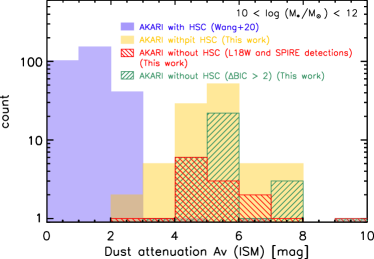
Figure 7: Histogram of the $V$-band attenuations in the ISM of AKARI sources with (blue) and without (yellow) HSC counterparts. The red line represents $A_{\rm V}^{\rm ISM}$ of our sample with L18W and SPIRE detections. Green line represents our sample with $\Delta$BIC $>$ 2.0. The objects with $10<\log\,(M_{*}/M_{\sun})<12$ are plotted in each sample.

We then compare the $V$-band attenuation in the ISM ($A_{\rm V}^{\rm ISM}$) for AKARI sources with and without HSC counterparts. Before the comparison, we should note that the dust attenuation may depend on the stellar mass (e.g., Buat et al., 2012, 2015), and the stellar mass distributions in the two samples are different as discussed in Section 4.1. Therefore, we extracted objects in an overlapped stellar mass range, i.e., $10<\log\,(M_{*}/M_{\sun})<12$ in the AKARI sample with/without HSC counterparts (see Figure 6).

Figure 7 shows the $V$-band attenuation in the ISM ($A_{\rm V}^{\rm ISM}$) for AKARI sources with and without HSC counterparts. These objects are stellar-mass matched samples. The average $A_{\rm V}^{\rm ISM}$ of AKARI sources with and without HSC counterparts is 1.26 and 5.16 mag, respectively. We find that the attenuation of our sample is systematically much larger than that of AKARI sources with HSC counterparts (Wang et al., 2020), which is supported by the K-S test with $>$99.9% significance. This result seems to be reasonable, given a fact that our sample is undetected even by the HSC, and its optical light is expected to be suppressed heavily by enshrouding dust.

One caution is that the redshift distributions of AKARI objects in Wang et al. (2020) and this study are different (see Section 4.3). Given an overlapped redshift range ($0.8<z<2.0$) between two samples (see Figure 8), the average $A_{\rm V}^{\rm ISM}$ of sample in Wang et al. (2020) and this work is 1.77 and 5.23 mag, respectively. This suggests that our sample is intrinsically affected by dust extinction compared with AKARI with HSC counterparts.

4.3 AGN Luminosity as a Function of Redshift

Figure 8 shows the IR luminosity contributed from AGN as a function of redshift. We find that AKARI objects without HSC counterparts tend to be located in higher redshifts compared to those with HSC counterparts: the mean redshift of AKARI objects with and without HSC counterparts is $z\sim$ 0.46 and 1.34, respectively. We also find that objects with L18W and SPIRE detections tend to have large AGN luminosity compared with others in our sample.

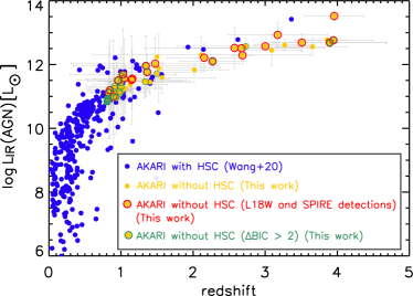
Figure 8: IR luminosity contributed from AGN as a function of redshift. Blue and yellow points represent AKARI sources with and without HSC counterparts, respectively. Yellow and red circles represent our sample with L18W and SPIRE detections. Yellow and green circles represent our sample with $\Delta$BIC $>$ 2.0.

Note that the parent sample for these objects is the same, i.e., a flux-limited sample drawn from the AKARI NEP-W catalog (Kim et al., 2012). Thus AKARI sources are expected to lie in the same sequence on the redshift–luminosity plane, regardless of HSC detection. We confirm that samples in Wang et al. (2020) and this work are continuously distributed in that plane, indicating that CIGALE securely estimated redshift and luminosity. Indeed, given the overlapped redshift range of $0.8<z<2.0$, the mean AGN luminosity of our sample is $\log(L_{\rm IR}{\rm(AGN)}/L_{\sun})\sim$ 11.2, is comparable to the sample in Wang et al. (2020).

The total IR luminosity of AKARI sources without HSC counterparts is also larger than those with HSC counterparts, with a mean $\log\,(L_{\rm IR}/L_{\sun})$ of 11.4 and 12.2, respectively. Actually, about 65% and 15% of our sample is ultra-luminous IR galaxies (ULIRGs: Sanders & Mirabel, 1996) and hyper-luminous IR galaxies (HyLIRGs: Rowan-Robinson, 2000) with $L_{\rm IR}$ greater than $10^{12}$ and $10^{13}$ $L_{\sun}$, respectively. This is in good agreement with a fact that dusty galaxies with extreme optical–IR color tend to be luminous in the IR (e.g., Tsai et al., 2015; Toba & Nagao, 2016; Toba et al., 2018; Fan et al., 2020; Toba et al., 2020b).

4.4 AGN fraction

Figure 9 shows the AGN fraction ($f_{\rm AGN}$), $L_{\rm IR}$ (AGN) / $L_{\rm IR}$. The mean AGN fraction of AKARI sources with and without HSC counterparts is 0.06 and 0.22, respectively, indicating our sample tends to harbor AGNs. We also find that $f_{\rm AGN}$ of objects with L18W and SPIRE detection is 0.16, smaller than average of all objects in our sample. On the other hand, given the overlapped redshift range ($0.8<z<2.0$), the mean $f_{\rm AGN}$ of AKARI sources with and without HSC counterparts is 0.12 and 0.23, respectively. This could indicate that one of the reasons for the difference in $f_{\rm AGN}$ between the two samples may be the difference in sample selection and redshift. Other possible uncertainties caused by a limited number of MIR data are discussed in Section 4.6.2.

Figure 9: Histograms of AGN fraction for AKARI sources with (blue) and without (yellow) HSC counterparts. The red line represents $f_{\rm AGN}$ of our sample with L18W and SPIRE detections. Green line represent $f_{\rm AGN}$ of our sample with BIC $>$ 2.0 (see Section 4.6.2).

4.5 Star Formation Rate

Finally, we compare the SFR in two samples as shown in Figure 10. The SFR is converted from dust luminosity using a relation provided by Kennicutt (1998) (see also Hirashita et al. 2003).

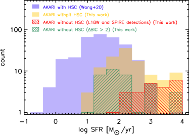
Figure 10: Histograms of SFR for AKARI sources with (blue) and without (yellow) HSC counterparts. The red and green lines represent the SFR of our sample with L18W and SPIRE detections, and with $\Delta$BIC $>$ 2.0, respectively.

We find that the SFR of our sample is systematically higher than that of AKARI with HSC objects. The average SFR of AKARI objects with and without HSC counterparts is about 91 and 758 $M_{\sun}$ yr^-1, respectively. If we focus on our sample with L18W and SPIRE detections, the mean SFR is 2240 $M_{\sun}$ yr^-1 because of requirement of FIR detection. These results are consistent with previous works reporting that SFRs of dusty galaxies tend to be high (e.g., Ikarashi et al., 2017; Toba et al., 2017b; Yamaguchi et al., 2019; Fan et al., 2020). On the other hand, if we compare SFRs of sample in this work and Wang et al. (2020) in an overlapped redshift range ($0.8<z<2.0$), the mean SFR of AKARI with and without HSC counterparts is 319 and 207 $M_{\sun}$ yr^-1, respectively. This indicates that the observed difference in SFR may be due to the redshift difference.

4.6 Reliability of the SED Analysis

4.6.1 Influence of Dataset without Optical Photometry on the SED-based Photometric Redshift

We showed that our estimate of $z_{\rm photo}$ is expected to be secure in some ways (see Sections 2.3 and 4.3), but these arguments are indirect. Although Małek et al. (2014) demonstrated the accuracy of $z_{\rm photo}$ based on CIGALE for an AKARI sample at $z_{\rm spec}<0.25$, they utilized optical data points for $z_{\rm photo}$ estimation, and the redshift range for the sample differs from our sample. We need to investigate how the lack of optical data affects the accuracy of $z_{\rm photo}$ for AKARI objects at $z>0.8$. Hence, we estimate $z_{\rm photo}$ of AKARI objects with $z_{\rm spec}$ in the band-merged catalog (S. J. Kim et al. 2020, in preparation). In order to calculate the $z_{\rm photo}$ under the same condition as we performed so far, we extracted objects with $z_{\rm spec}>0.8$ and with 5-band detections in NIR-FIR, yielding 100 objects. Note that although the sample is detected by the HSC, we “artificially” multiplied the HSC flux densities by 10 and treated them as 10$\sigma$ upper limits. We then executed the SED fitting with CIGALE in the exactly same manner as what we described in Section 2.3.

Figure 11: Relative difference between $z_{\rm photo}$ and $z_{\rm spec}$, $(z_{\rm spec}-z_{\rm photo})/(1+z_{\rm spec})$ as a function of $z_{\rm spec}$.The red solid line represents $z_{\rm photo}-z_{\rm spec}=0$ and the dotted lines represent $(z_{\rm spec}-z_{\rm photo})/(1+z_{\rm spec})=\pm 0.2$. The inserted panel shows the histogram of $(z_{\rm spec}-z_{\rm photo})/(1+z_{\rm spec})$.

Figure 11 shows the relative difference between $z_{\rm photo}$ and $z_{\rm spec}$, i.e., $(z_{\rm spec}-z_{\rm photo})/(1+z_{\rm spec})$ as a function of $z_{\rm spec}$. The mean and standard deviation of $(z_{\rm spec}-z_{\rm photo})/(1+z_{\rm spec})$ is $0.09\pm 0.45$, and the accuracy of $z_{\rm photo}$, $\sigma_{\Delta z/(1+z_{\rm spec})}$ is 0.23, which are worse than those reported by Małek et al. (2014). We find that $\sim 56$% of objects have $|(z_{\rm spec}-z_{\rm photo})|/(1+z_{\rm spec})$ $<0.2$. This may be partly because the AKARI–HSC objects at $z>0.8$ are biased toward optically-bright type 1 AGNs, for which $z_{\rm photo}$ is harder to estimate precisely, compared with other galaxy types. Actually, $\sim 90$% of objects plotted in Figure 11 are spectroscopically confirmed type 1 AGNs, which may induce a large deviation of $(z_{\rm spec}-z_{\rm photo})/(1+z_{\rm spec})$.

4.6.2 Bayesian Information Criterion

An another potential issue raised by the SED fitting with a limited number of data points in the MIR may be an uncertainty of AGN contribution to the total SED, although we used upper-limits at a MIR band if an object is not detected at that band. To test the requirement to add an AGN component to the SED fitting, we compute the Bayesian information criterion (BIC) for two fits that are derived with and without AGN component. The BIC is defined as BIC = $\chi^{2}$ + $k$ $\times$ ln($n$), where $\chi^{2}$ is non-reduced chi-square, $k$ is the number of degrees of freedom (DOF), and $n$ is the number of photometric data points used for the fitting, respectively. We then compare the results of two SED fittings without/with AGN module by using $\Delta$BIC = BIC_woAGN – BIC_wAGN. The resultant $\Delta$BIC tells whether the AGN model is required to give a better fit with taking into account the difference in DOF (e.g., Ciesla et al., 2018; Buat et al., 2019, see also Aufort et al. 2020).

Figure 12: Histogram of $\Delta$BIC = BIC_woAGN–BIC_wAGN for AKARI sources without HSC counterparts. The red dotted line corresponds to $\Delta$BIC = 2.

Figure 12 shows the histogram of $\Delta$BIC for AKARI sources without HSC counterparts. If $\Delta$BIC is larger than two, this indicates that adding the AGN component provides a better fit than without adding it (Liddle, 2004; Stanley et al., 2015) (see also Ciesla et al. 2018; Buat et al. 2019 who set a higher threshold for $\Delta$BIC). Otherwise, there is no significant difference between two fits with/without AGN model. We find that only 31% of object fits satisfy $\Delta$BIC $>2$. This suggests it may be difficult to constrain the AGN activity for many cases, and thus AGN fraction may have a large uncertainty given a limited number of photometric detections in the MIR regime. On the other hand, Figures 6–10 also show objects with $\Delta$BIC $>2$. We find that there is no systematic difference between objects with $\Delta$BIC $>2$ and others, especially for AGN fraction (see Figure 9), which suggests that overall trends discussed in Section 4.4 may not be changed even if taking into account the BIC.

4.6.3 Mock Analysis

Finally, we check whether or not the derived physical properties in this work can actually be estimated reliably, given the uncertainty of the photometry. We conduct a mock analysis that is a procedure provided by CIGALE (see e.g., Buat et al., 2012, 2014; Ciesla et al., 2015; Lo Faro et al., 2017; Boquien et al., 2019; Toba et al., 2019b, for more detail).

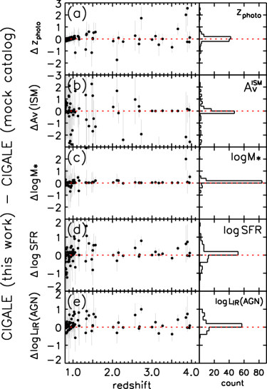
Figure 13: The differences in $z_{\rm photo}$, $V$-band attenuation in the ISM, stellar mass, SFR, and $L_{\rm IR}$(AGN) derived from CIGALE in this work and those derived from the mock catalog. (a) $\Delta z_{\rm photo}$, (b) $\Delta A_{\rm V}^{\rm ISM}$, (c) $\Delta\log\,M_{*}$, (d) $\Delta\log{\rm SFR}$, and (e) $\Delta\log L_{\rm IR}$(AGN) as a function of redshift. The right panels show a histogram of each quantity. The red dotted lines are the $\Delta$= 0.

Figure 13 shows the differences in $z_{\rm photo}$, $V$-band attenuation in the ISM ($A_{\rm V}$), stellar mass, SFR, and $L_{\rm IR}$(AGN) derived from CIGALE in this work and those derived from the mock catalog as a function of redshift. The mean and standerd deviations of $\Delta z_{\rm photo}$, $\Delta A_{\rm V}^{\rm ISM}$, $\Delta\log\,M_{*}$, $\Delta\log{\rm SFR}$, and $\Delta\log L_{\rm IR}$(AGN) are $\Delta z_{\rm photo}=0.03\pm 0.47$, $\Delta A_{\rm V}^{\rm ISM}=-0.23\pm 1.17$, $\Delta\log\,M_{*}=0.08\pm 0.37$, $\Delta\log{\rm SFR}=0.03\pm 0.43$, and $\Delta\log L_{\rm IR}$(AGN) = 0.11 $\pm$ 0.30, respectively. In particular, we can see a large deviation for objects at $z<1.5$. This trend can also be seen in Figure 11. These results indicate that any physical quantities derived by the SED fitting especially for objects at $z<1.5$ may be significantly affected by the limited number of photometric data points. On the other hand, we could ensure reliable physical quantities for our sample at $z>1.5$.

5 Summary

In this paper, we report the physical properties of AKARI sources that do not have optical counterparts in the HSC/Subaru catalog (Oi et al., 2020). The parent sample is drawn from IR sources in the AKARI NEP-W field (Kim et al., 2012). By using AKARI, HSC, Gaia, FLAMINGOS/KPNO and IRAC/Spitzer catalogs and images, we select 583 objects as optically-dark IR sources without HSC counterparts. Thanks to the continuous filters of AKARI in the MIR and multi-wavelength data up to the FIR (SPIRE/Herschel), we successfully pin down their optical–FIR SEDs, even if flux densities in some bands are upper limits. We compare the physical properties derived by the CIGALE SED fitting between AKARI objects without HSC counterparts and mid-IR selected AKARI objects with HSC counterparts (Wang et al., 2020). We find that AKARI sources without HSC counterparts have systematically redder 3.6 $-$ 4.5 $\micron$ color compared with AKARI sources with HSC counterparts. With all the caveats discussed in Section 4.6 in mind, we find that our sample tends to be located at high redshifts up to $z\sim 4$, and has larger AGN luminosity, SFR, and $V$-band dust attenuation in the ISM, compared with AKARI sources with HSC counterparts. Although this is partly due to the Malmquist bias, these results indicate that AKARI objects without HSC counterparts are heavily dust-obscured SFGs/AGNs at $z\sim$ 1-4 that may be missed by the previous optical surveys.

The launch of the James Webb Space Telescope (JWST: Gardner et al., 2006) is approaching, and AKARI NEP should be an attractive field for JWST (e.g., Jansen & Windhorst, 2018). Since the AKARI NEP has multi-wavelength data from X-ray to radio, in which the filter sets of AKARI are similar to those of JWST, this work establishes a benchmark for forthcoming dusty SFGs/AGNs studies with JWST and provides specially interesting optically dark IR sources for JWST study.

References

- Aird et al. (2015) Aird, J., Coil, A. L., Georgakakis, A., et al. 2015, MNRAS, 451, 1892
- Aufort et al. (2020) Aufort, G., Ciesla, L, Pudlo, P., & Buat, V. 2020, A&A, 635, A136
- Barrufet et al. (2020) Barrufet, L., Pearson, C., Serjeant, S., et al. 2020, A&A, submitted.
- Bertin & Arnouts (1996) Bertin, E., & Arnouts, S. 1996, \aas, 117, 393
- Blecha et al. (2018) Blecha, L., Snyder, G. F., Satyapal, S., & Ellison, S. L. 2018, MNRAS, 478, 3056
- Boquien et al. (2014) Boquien, M., Buat, V., & Perret, V. 2014, A&A, 571, A72
- Boquien et al. (2016) Boquien, M., Kennicutt, R., Calzetti, D., et al. 2016, A&A, 591, A6
- Boquien et al. (2019) Boquien, M., Burgarella, D., Roehlly, Y., et al. 2019, A&A, 622, A103
- Boulade et al. (2003) Boulade, O., Charlot, X., Abbon, P., et al. 2003, Proc. SPIE, 4841, 72
- Bosch et al. (2018) Bosch, J., Armstrong, R., Bickerton, S., et al. 2018, PASJ, 70, S5
- Bruzual & Charlot (2003) Bruzual, G., & Charlot, S. 2003, MNRAS, 344, 1000
- Buat et al. (2012) Buat, V., Noll, S., Burgarella, D., et al. 2012, A&A, 545, A141
- Buat et al. (2014) Buat, V., Heinis, S., Boquien, M., et al. 2014, A&A, 561, A39
- Buat et al. (2015) Buat, V., Oi, N., Heinis, S., et al. 2015, A&A, 577, A141
- Buat et al. (2017) Buat, V., Oi, N., Burgarella, D., et al. 2017, Publication of Korean Astronomical Society, 32, 257
- Buat et al. (2019) Buat, V., Ciesla, L., Boquien, M., Małek, K., & Burgarella, D. 2019, A&A, 632, A79
- Burgarella et al. (2005) Burgarella, D., Buat, V., & Iglesias-Páramo, J. 2005, MNRAS, 360, 1413
- Burgarella et al. (2020) Burgarella D., Nanni A., Hirashita H., et al. 2020, A&A, 637, A32
- Casey et al. (2014) Casey, C. M., Narayanan, D., & Cooray, A. 2014, Phys. Rep., 541, 45
- Charlot & Fall (2000) Charlot, S., & Fall, S. M. 2000, ApJ, 539, 718
- Chen et al. (2020) Chen, X-Y., Akiyama, M., Ichikawa, K., et al. 2020, arXiv:1911.04095
- Chiang et al. (2019) Chiang, C-Y., Goto.T., Hashimoto.T., et al. 2019. PASJ, 71, 31
- Ciesla et al. (2015) Ciesla, L., Charmandaris, V., Georgakakis, A., et al. 2015, A&A, 576, A10
- Ciesla et al. (2016) Ciesla, L., Boselli, A., Elbaz, D., et al. 2016, A&A, 585, A43
- Ciesla et al. (2017) Ciesla, L., Elbaz, D., & Fensch, J. 2017, A&A, 608, A41
- Ciesla et al. (2018) Ciesla, L., Elbaz, D., Schreiber, C., Daddi, E., & Wang, T. 2018, A&A, 615, A61
- Dey et al. (2008) Dey, A., Soifer, B. T., Desai, V., et al. 2008, ApJ, 677, 943
- Draine et al. (2014) Draine, B. T., Aniano, G., Krause, O., et al. 2014, ApJ, 780, 172
- Eisenhardt et al. (2012) Eisenhardt, P. R. M., Wu, J., Tsai, C.-W., et al. 2012, ApJ, 755, 173
- Ellison et al. (2019) Ellison, S. L., Viswanathan, A., Patton, D. R., et al. 2019, MNRAS, 487, 2491
- Elston et al. (2006) Elston, R. J., Gonzalez, A. H., McKenzie, E., et al. 2006, ApJ, 639, 816
- Fan et al. (2020) Fan, L., Knudsen, K. K., Han, Y., & Tan, Q-H, 2020, ApJ, 887, 74
- Fazio et al. (2004) Fazio, G. G., Hora, J. L., Allen, L. E., et al. 2004, ApJS, 154, 10
- Franco et al. (2018) Franco, M., Elbaz, D., Béthermin, M., et al. 2018, A&A, 620, A152
- Fritz et al. (2006) Fritz, J., Franceschini, A., & Hatziminaoglou, E. 2006, MNRAS, 366, 767
- Furusawa et al. (2018) Furusawa, H., Koike, M., Takata, T., et al. 2018, PASJ, 70, S3
- Gaia Collaboration (2016) Gaia Collaboration, Brown, A. G. A., Vallenari, A., et al. 2016, A&A, 595, A2
- Gaia Collaboration (2018) Gaia Collaboration, Brown, A. G. A., Vallenari, A., et al. 2018, A&A, 616, A1
- Gao et al. (2020) Gao, F., Wang, L., Pearson, W. J., et al. 2020, A&A, 637, A94
- Gardner et al. (2006) Gardner, J. P., Mather, J. C., Clampin, M., et al. 2006, Space Sci. Rev., 123, 485
- Goto et al. (2011) Goto, T., Arnouts, S., Inami, H., et al. 2011, MNRAS, 410, 573
- Goto et al. (2019) Goto, T., Oi, N., Utsumi, Y., et al. 2019, PASJ, 71, 30
- Griffin et al. (2010) Griffin, M. J., Abergel, A., Abreu, A., et al. 2010, A&A, 518, L3
- Hickox & Alexander (2018) Hickox, R. C., & Alexander, D. M. 2018, ARA&A, 56, 625
- Hirashita et al. (2003) Hirashita, H., Buat, V., & Inoue, A. K. 2003, A&A, 410, 83
- Ho et al. (2020) Ho, C-C., Goto, T., Oi, N., et al. 2020, MNRAS, submitted
- Hopkins et al. (2008) Hopkins, P. F., Hernquist, L., Cox, T. J., & Kereš, D. 2008, ApJS, 175, 356
- Huang et al. (2017) Huang, T., Goto, T., Hashimoto, T., et al. 2017, MNRAS, 471, 4239
- Hwang et al. (2013a) Hwang, H. S., Andrews, S. M., & Geller, M. J. 2013, ApJ, 777, 38
- Hwang et al. (2013b) Hwang, H. S., & Geller, M. J. 2013, ApJ, 769, 116
- Hwang et al. (2007) Hwang, N., Lee, M. G., Lee, H. M., et al. 2007, ApJS, 172, 583
- Ikarashi et al. (2017) Ikarashi, S., Caputi, K. I., Ohta, K., et al. 2017, ApJ, 849, L36
- Ilbert et al. (2006) Ilbert, O., Arnouts, S., McCracken, H. J., et al. 2006, A&A, 457, 841
- Im et al. (2010) Im, M., Ko, J., Cho, Y., et al. 2010, J. Korean Astron. Soc., 43, 75
- Inoue (2011) Inoue, A. K. 2011, MNRAS, 415, 2920
- Ishihara et al. (2010) Ishihara, D., Onaka, T., Kataza, H., et al. 2010, A&A, 514, 1
- Jansen & Windhorst (2018) Jansen R. A., & Windhorst R. A., 2018, PASP, 130, 124001
- Jeon et al. (2014) Jeon, Y., Im, M., Kang, E., Lee, H. M., & Matsuhara, H. 2014, ApJS, 214, 20
- Jeon et al. (2010) Jeon, Y., Im, M., Ibrahimov, M., et al. 2010, ApJS, 190, 166
- Kawanomoto et al. (2018) Kawanomoto, S., Uraguchi, F., Komiyama, Y., et al. 2018, PASJ, 70, 66
- Kennicutt (1998) Kennicutt, R. C., Jr. 1998, ARA&A, 36, 189
- Kim et al. (2018) Kim, H. K., Malkan, M. A., Oi, N., et al. 2018, in Ootsubo T., Yamamura I., Murata K., Onaka T., eds, The Cosmic Wheel and the Legacy of the AKARI Archive: From Galaxies and Stars to Planets and Life. pp 371-374
- Kim et al. (2012) Kim, S. J., Lee, H. M., Matsuhara, H., et al. 2012, A&A, 548, A29
- Kim et al. (2019) Kim, S. J., Jeong, W-S., Goto.T., et al. 2019, PASJ, 71, 11
- Komatsu et al. (2011) Komatsu, E., Smith, K. M., Dunkley, J., et al. 2011, ApJS, 192, 18
- Komiyama et al. (2018) Komiyama, Y., Obuchi, Y., Nakaya, H., et al. 2018, PASJ, 70, S2
- Krumpe et al. (2015) Krumpe, M., Miyaji, T., Brunner, H., et al. 2015, MNRAS, 446, 911
- Landsman (1993) Landsman, W. B. 1993, in ASP Conf. Ser. 52, Astronomical Data Analysis Software and Systems II, ed. R. J. Hanisch, R. J. V. Brissenden, & J. Barnes (San Francisco, CA: ASP), 246
- Lee et al. (2009) Lee, H. M., Kim, S. J., Im, M., et al. 2009, PASJ, 61, 375
- Liddle (2004) Liddle, A. R. 2004, MNRAS, 351, L49
- Lo Faro et al. (2017) Lo Faro, B., Buat, V., Roehlly, Y., et al. 2017, MNRAS, 472, 1372
- Madau & Dickinson (2014) Madau, P., & Dickinson, M. 2014, ARA&A, 52, 415
- Małek et al. (2014) Małek, K., Pollo, A., Takeuchi, T. T., et al. 2014, A&A, 562, A15
- Matsuhara et al. (2006) Matsuhara, H., Wada, T., Matsuura, S., et al. 2006, PASJ, 58, 673
- Melbourne et al. (2012) Melbourne, J., Soifer, B. T., Desai, V., et al. 2012, AJ, 143, 125
- Miyazaki et al. (2018) Miyazaki, S., Komiyama, Y., Kawanomoto, S., et al. 2018, PASJ, 70, S1
- Murakami et al. (2007) Murakami, H., Baba, H., Barthel, P., et al. 2007, PASJ, 59, S369
- Murata et al. (2013) Murata, K., Matsuhara, H., Wada, T., et al. 2013, A&A, 559, A132
- Murata et al. (2014) Murata, K., Matsuhara, H., Inami, H., et al. 2014, A&A, 566, A136
- Narayanan et al. (2010) Narayanan, D., Dey, A., Hayward, C. C., et al. 2010, MNRAS, 407, 1701
- Nayyeri et al. (2018) Nayyeri, H., Ghotbi, N., Cooray, A., et al. 2018, ApJS, 234, 38
- Noboriguchi et al. (2019) Noboriguchi, A., Nagao, T., Toba, Y., et al. 2019, ApJ, 876, 132
- Noll et al. (2009) Noll, S., Burgarella, D., Giovannoli, E., et al. 2009, A&A, 507, 3
- Oi et al. (2017) Oi, N., Goto, T., Malkan, M., Pearson, C., & Matsuhara, H. 2017, PASJ, 69, 70
- Oi et al. (2020) Oi, N., Goto, T., Matsuhara, H., et al. 2020, MNRAS, submitted
- Onaka et al. (2007) Onaka, T., Matsuhara, H., Wada, K., et al. 2007, PASJ, 59, S401
- Pearson et al. (2017) Pearson, C., Cheale, R., Serjeant, S., et al. 2017, PKAS, 32, 219
- Pearson et al. (2019) Pearson, C., Barrufet, L., Campos Varillas, M. d. C., et al. 2019, PASJ, 71, 13
- Pilbratt et al. (2010) Pilbratt, G. L., Riedinger, J. R., Passvogel, T., et al. 2010, A&A, 518, L1
- Poglitsch et al. (2010) Poglitsch, A., Waelkens, C., Geis, N., et al. 2010, A&A, 518, L2
- Poliszczuk et al. (2019) Poliszczuk, A., Solarz, A., Pollo, A., et al. 2019, PASJ, 71, 65
- Ricci et al. (2017) Ricci, C., Bauer, F. E., Treister, E., et al. 2017, MNRAS, 468, 1273
- Riguccini et al. (2019) Riguccini, L. A., Treister, E., Menéndez-Delmestre, K., et al. 2019, AJ, 157, 233
- Rowan-Robinson (2000) Rowan-Robinson, M. 2000, MNRAS, 316, 885
- Salpeter (1955) Salpeter, E. E. 1955, ApJ, 121, 161
- Sanders & Mirabel (1996) Sanders, D. B., & Mirabel, I. F. 1996, ARA&A, 34, 749
- Sawicki (2012) Sawicki, M. 2012, PASP, 124, 1208
- Schwarz (1978) Schwarz, G. 1978, The Annals of Statistics, 6, 461
- Shim et al. (2013) Shim, H., Im, M., Ko, J., et al. 2013, ApJS, 207, 37
- Shogaki et al. (2018) Shogaki, A., Matsuura, S., Oi, N., et al. 2018, in Ootsubo T., Yamamura I., Murata K., Onaka T., eds, The Cosmic Wheel and the Legacy of the AKARI Archive: From Galaxies and Stars to Planets and Life. pp 367-370
- Stanley et al. (2015) Stanley, F., Harrison, C. M., Alexander, D. M., et al. 2015, MNRAS, 453, 591
- Takagi et al. (2010) Takagi, T., Oyama, Y., Goto, T., et al. 2010, A&A, 514, A5
- Taylor (2006) Taylor, M. B. 2006, in ASP Conf. Ser. 351, Astronomical Data Analysis Software and Systems XV, ed. C. Gabriel et al. (San Francisco, CA: ASP), 666
- Toba et al. (2015) Toba, Y., Nagao, T., Strauss, M. A., et al. 2015, PASJ, 67, 86
- Toba & Nagao (2016) Toba, Y., & Nagao, T. 2016, ApJ, 820, 46
- Toba et al. (2017a) Toba, Y., Nagao, T., Kajisawa, M., et al. 2017a, ApJ, 835, 36
- Toba et al. (2017b) Toba, Y., Nagao, T., Wang, W-H., et al. 2017b, ApJ, 840, 21,
- Toba et al. (2017c) Toba, Y., Bae, H-J., Nagao, T., et al. 2017c, ApJ, 850, 140
- Toba et al. (2017d) Toba, Y., Komugi, S., Nagao, T., et al. 2017d, ApJ, 851, 98
- Toba et al. (2018) Toba Y., Ueda J., Lim C.-F., et al. 2018, ApJ, 857, 31
- Toba et al. (2019a) Toba, Y., Ueda, Y., Matsuoka, K., et al. 2019a, MNRAS, 484, 196
- Toba et al. (2019b) Toba, Y., Yamashita, T., Nagao, T., et al. 2019b, ApJS, 243, 15
- Toba et al. (2020a) Toba, Y., Yamada, S., Ueda, Y., et al. 2020a, ApJ, 888, 8
- Toba et al. (2020b) Toba, Y., Wang, W-H., Nagao, T., et al. 2020b, ApJ, 889, 76
- Tsai et al. (2015) Tsai, C.-W., Eisenhardt, P. R. M., Wu, J., et al. 2015, ApJ, 805, 90
- Ueda et al. (2014) Ueda, Y., Akiyama, M., Hasinger, G., Miyaji, T., & Watson, M. G. 2014, ApJ, 786, 104
- Wada et al. (2008) Wada, T., Matsuhara, H., Oyabu, S., et al. 2008, PASJ, 60, S517
- Wang et al. (2019) Wang, T., Schreiber, C., Elbaz, D., et al. 2019, Nature, 572, 211
- Wang et al. (2020) Wang, T-W., Goto, T., Kim, S. J., et al. 2020, MNRAS, submitted
- Werner et al. (2004) Werner, M. W., Roellig, T. L., Low, F. J., et al. 2004, ApJS, 154, 1
- Williams et al. (2019) Williams, C. C., Labbe, I., Spilker, J., et al. 2019, ApJ, 884, 154
- White et al. (2010) White, G. J., Pearson, C., Braun, R., et al. 2010, A&A, 517, A54
- Wright et al. (2010) Wright, E. L., Eisenhardt, P. R. M., Mainzer, A. K., et al. 2010, AJ, 140, 1868
- Wu et al. (2012) Wu, J., Tsai, C.-W., Sayers, J., et al. 2012, ApJ, 756, 96
- Yamaguchi et al. (2019) Yamaguchi, Y., Kohno, K., Hatsukade, B., et al. 2019, ApJ, 878, 73
- Yamamura et al. (2010) Yamamura, I., Makiuti, S., Ikeda, N., et al. 2010, yCat, 2298, 0