Primal-dual path-following methods and the trust-region updating strategy for linear programming with noisy data

Abstract

In this article, we consider the primal-dual path-following method and the trust-region updating strategy for the standard linear programming problem. For the rank-deficient problem with the small noisy data, we also give the preprocessing method based on the QR decomposition with column pivoting. Then, we prove the global convergence of the new method when the initial point is strictly primal-dual feasible. Finally, for some rank-deficient problems with or without the small noisy data from the NETLIB collection, we compare it with other two popular interior-point methods, i.e. the subroutine pathfollow.m and the built-in subroutine linprog.m of the MATLAB environment. Numerical results show that the new method is more robust than the other two methods for the rank-deficient problem with the small noise data.

1 Introduction

In this article, we are mainly concerned with the linear programming problem with the small noisy data as follows:

$$\min_{x\in\Re^{n}}c^{T}x,\hskip 5.69054pt\text{subject to}\;Ax=b,\;x\geq 0,$$ (1)

where $c$ and $x$ are vectors in $\Re^{n}$, $b$ is a vector in $\Re^{m}$, and $A$ is an $m\times n$ matrix. For the problem (1), there are many efficient methods to solve it such as the simplex methods Pan2010 ; ZYL2013 , the interior-point methods FMW2007 ; Gonzaga1992 ; NW1999 ; Wright1997 ; YTM1994 ; Zhang1998 and the continuous methods AM1991 ; CL2011 ; Monteiro1991 ; Liao2014 . Those methods are all assumed that the constraints of problem (1) are consistent, i.e. $rank(A,\,b)=rank(A)$. For the consistent system of redundant constraints, references AA1995 ; Andersen1995 ; MS2003 provided a few preprocessing strategies which are widely used in both academic and commercial linear programming solvers.

However, for a real-world problem, since it may include the redundant constraints and the measurement errors, the rank of matrix $A$ may be deficient and the right-hand-side vector $b$ has small noise. Consequently, they may lead to the inconsistent system of constraints AZ2008 ; CI2012 ; LLS2020 . On the other hand, the constraints of the original real-world problem are intrinsically consistent. Therefore, we consider the least-squares approximation of the inconsistent constraints in the linear programming problem based on the QR decomposition with column pivoting. Then, according to the first-order KKT conditions of the linear programming problem, we convert the processed problems into the equivalent problem of nonlinear equations with nonnegative constraints. Based on the system of nonlinear equations with nonnegative constraints, we consider a special continuous Newton flow with nonnegative constraints, which has the nonnegative steady-state solution for any nonnegative initial point. Finally, we consider a primal-dual path-following method and the adaptive trust-region updating strategy to follow the trajectory of the continuous Newton flow. Thus, we obtain an optimal solution of the original linear programming problem.

The rest of this article is organized as follows. In the next section, we consider the primal-dual path-following method and the adaptive trust-region updating strategy for the linear programming problem. In section 3, we analyze the global convergence of the new method when the initial point is strictly primal-dual feasible. In section 4, for the rank-deficient problems with or without the small noise, we compare the new method with two other popular interior-point methods, i.e. the traditional path-following method (pathfollow.m in p. 210, FMW2007 ) and the predictor-corrector algorithm (the built-in subroutine linprog.m of the MATLAB environment MATLAB ; Mehrotra1992 ; Zhang1998 ). Numerical results show that the new method is more robust than the other two methods for the rank-deficient problem with the small noisy data. Finally, some discussions are given in section 5. $\|\cdot\|$ denotes the Euclidean vector norm or its induced matrix norm throughout the paper.

2 Primal-dual path-following methods and the trust-region updating strategy

2.1 The continuous Newton flow

For the linear programming problem (1), it is well known that its optimal solution $x^{\ast}$ if and only if it satisfies the following Karush-Kuhn-Tucker conditions (pp. 396-397, NW1999 ):

$$Ax-b=0,\;A^{T}y+s-c=0,\;XSe=0,\;(x,\,s)\geq 0,$$ (2)

where

$$X=diag(x),\;S=diag(s),\;\text{and}\;e=(1,\,\ldots,\,1)^{T}.$$ (3)

For convenience, we rewrite the optimality condition (2) as the following nonlinear system of equations with nonnegative constraints:

$$F(z)=\begin{bmatrix}Ax-b\\ A^{T}y+s-c\\ XSe\end{bmatrix}=0,\;(x,\,s)\geq 0,\;\text{and}\;z=(x,\,y,\,s).$$ (4)

It is not difficult to know that the Jacobian matrix $J(z)$ of $F(z)$ has the following form:

$$J(z)=\begin{bmatrix}A&0&0\\ 0&A^{T}&I\\ S&0&X\end{bmatrix}.$$ (5)

From the third block $XSe=0$ of equation (4), we know that $x_{i}=0$ or $s_{i}=0\,(i=1:n)$. Thus, the Jacobian matrix $J(z)$ of equation (5) may be singular, which leads to numerical difficulties near the solution of the nonlinear system (4) for the Newton’s method or its variants. In order to overcome this difficulty, we consider its perturbed system AG2003 ; Tanabe1988 as follows:

$$F_{\mu}(z)=F(z)-\begin{bmatrix}0\\ 0\\ \mu e\end{bmatrix}=0,\;(x,\,s)>0,\;\mu>0\;\text{and}\;z=(x,\,y,\,s).$$ (6)

The solution $z(\mu)$ of the perturbed system (6) defines the primal-dual central path, and $z(\mu)$ approximates the solution $z^{\ast}$ of the nonlinear system (4) when $\mu$ tends to zero FMW2007 ; NW1999 ; Wright1997 ; Ye1997 .

We define the strictly feasible region $\mathbb{F}^{0}$ of the problem (1) as

$$\mathbb{F}^{0}=\left\{(x,\,y,\,s)|Ax=b,\;A^{T}y+s=c,\;(x,\,s)>0\right\}.$$ (7)

Then, when there is a strictly feasible interior point $(\bar{x},\,\bar{y},\,\bar{s})\in\mathbb{F}^{0}$ and the rank of matrix $A$ is full, the perturbed system (6) has a unique solution (Theorem 2.8, p. 39, Wright1997 ). The existence of its solution can be derived by the implicit theorem Doedel2007 and the uniqueness of its solution can be proved via considering the strict convexity of the following penalty problem and the KKT conditions of its optimal solution FM1990 :

$$\min c^{T}x-\mu\sum_{i=1}^{n}\log(x_{i})\;\text{subject to}\;Ax=b,$$ (8)

where $\mu$ is a positive parameter.

According to the duality theorem of the linear programming (Theorem 13.1, pp. 368-369, NW1999 ), for any primal-dual feasible solution $(x,\,y,\,s)$, we have

$$c^{T}x\geq b^{T}y^{\ast}=c^{T}x^{\ast}\geq b^{T}y,$$ (9)

where the triple $(x^{\ast},\,y^{\ast},\,s^{\ast})$ is a primal-dual optimal solution. Moreover, when the positive number $\mu$ is small, the solution $z^{\ast}(\mu)$ of perturbed system (6) is an approximation solution of nonlinear system (4). Consequently, from the duality theorem (9), we know that $x^{\ast}(\mu)$ is an approximation of the optimal solution of the original linear programming problem (1). It can be proved as follows. Since $z^{\ast}(\mu)$ is the primal-dual feasible, from inequality (9), we have

$$c^{T}x^{\ast}(\mu)\geq b^{T}y^{\ast}=c^{T}x^{\ast}\geq b^{T}y^{\ast}(\mu)$$ (10)

and

$$0\leq(x^{\ast}(\mu))^{T}s^{\ast}(\mu)=c^{T}x^{\ast}(\mu)-b^{T}y^{\ast}(\mu).$$ (11)

From equations (10)-(11), we obtain

$$|c^{T}x^{\ast}(\mu)-c^{T}x^{\ast}|\leq c^{T}x^{\ast}(\mu)-b^{T}y^{\ast}(\mu)=(x^{\ast}(\mu))^{T}s^{\ast}(\mu)=n\mu.$$ (12)

Therefore, $x^{\ast}(\mu)$ is an approximation of the optimal solution of the original linear programming problem (1).

If the damped Newton method is applied to the perturbed system (6) DS2009 ; NW1999 , we have

$$z_{k+1}=z_{k}-\alpha_{k}J(z_{k})^{-1}F_{\mu}(z_{k}),$$ (13)

where $J(z_{k})$ is the Jacobian matrix of $F_{\mu}(z)$. We regard $z_{k+1}=z(t_{k}+\alpha_{k}),\;z_{k}=z(t_{k})$ and let $\alpha_{k}\to 0$, then we obtain the continuous Newton flow with the constraints AS2015 ; Branin1972 ; Davidenko1953 ; Tanabe1979 ; LXL2020 of the perturbed system (6) as follows :

$$\frac{dz(t)}{dt}=-J(z)^{-1}F_{\mu}(z),\hskip 5.69054ptz=(x,\,y,\,s)\;\text{and}\;(x,\,s)>0.$$ (14)

Actually, if we apply an iteration with the explicit Euler method SGT2003 ; YFL1987 for the continuous Newton flow (14), we obtain the damped Newton method (13).

Since the Jacobian matrix $J(z)=F^{\prime}_{\mu}(z)$ may be singular, we reformulate the continuous Newton flow (14) as the following general formula Branin1972 ; Tanabe1979 :

$$-J(z)\frac{dz(t)}{dt}=F_{\mu}(z),\hskip 5.69054ptz=(x,\,y,\,s)\;\text{and}\;(x,\,s)>0.$$ (15)

The continuous Newton flow (15) has some nice properties. We state one of them as the following property 1 Branin1972 ; LXL2020 ; Tanabe1979 .

Property 1

(Branin Branin1972 and Tanabe Tanabe1979 ) Assume that $z(t)$ is the solution of the continuous Newton flow (15), then $f(z(t))=\|F_{\mu}(z)\|^{2}$ converges to zero when $t\to\infty$. That is to say, for every limit point $z^{\ast}$ of $z(t)$, it is also a solution of the perturbed system (6). Furthermore, every element $F_{\mu}^{i}(z)$ of $F_{\mu}(z)$ has the same convergence rate $exp(-t)$ and $z(t)$ can not converge to the solution $z^{\ast}$ of the perturbed system (6) on the finite interval when the initial point $z_{0}$ is not a solution of the perturbed system (6).

Proof.  Assume that $z(t)$ is the solution of the continuous Newton flow (15), then we have

$$\frac{d}{dt}\left(exp(t)F_{\mu}(z)\right)=exp(t)J(z)\frac{dz(t)}{dt}+exp(t)F_{\mu}(z)=0.$$

Consequently, we obtain

$$F_{\mu}(z(t))=F_{\mu}(z_{0})exp(-t).$$ (16)

From equation (16), it is not difficult to know that every element $F_{\mu}^{i}(z)$ of $F_{\mu}(z)$ converges to zero with the linear convergence rate $exp(-t)$ when $t\to\infty$. Thus, if the solution $z(t)$ of the continuous Newton flow (15) belongs to a compact set, it has a limit point $z^{\ast}$ when $t\to\infty$, and this limit point $z^{\ast}$ is also a solution of the perturbed system (6).

If we assume that the solution $z(t)$ of the continuous Newton flow (15) converges to the solution $z^{\ast}$ of the perturbed system (6) on the finite interval $(0,\,T]$, from equation (16), we have

$$F_{\mu}(z^{\ast})=F_{\mu}(z_{0})exp(-T).$$ (17)

Since $z^{\ast}$ is a solution of the perturbed system (6), we have $F_{\mu}(z^{\ast})=0$. By substituting it into equation (17), we obtain

$$F_{\mu}(z_{0})=0.$$

Thus, it contradicts the assumption that $z_{0}$ is not a solution of the perturbed system (6). Consequently, the solution $z(t)$ of the continuous Newton flow (15) can not converge to the solution $z^{\ast}$ of the perturbed system (6) on the finite interval. ∎

Remark 1

The inverse $J(x)^{-1}$ of the Jacobian matrix $J(x)$ can be regarded as the preconditioner of $F_{\mu}(x)$ such that the every element $x^{i}(t)$ of $x(t)$ has roughly the same convergence rate and it mitigates the stiffness of the ODE (15) LXL2020 . This property is very useful since it makes us adopt the explicit ODE method to follow the trajectory of the Newton flow (15) efficiently.

2.2 The primal-dual path-following method

From property 1, we know that the continuous Newton flow (15) has the nice global convergence property. However, when the Jacobian matrix $J(x)$ is singular or nearly singular, the ODE (15) is the system of differential-algebraic equations AP1998 ; BCP1996 ; HW1996 and its trajectory can not be efficiently followed by the general ODE method such as the backward differentiation formulas (the built-in subroutine ode15s.m of the MATLAB environment MATLAB ; SGT2003 ). Thus, we need to construct the special method to solve this problem. Furthermore, we expect that the new method has the global convergence as the homotopy continuation methods AG2003 ; OR2000 and the fast convergence rate as the traditional optimization methods. In order to achieve these two aims, we consider the continuation Newton method and the trust-region updating strategy for problem (15).

We apply the implicit Euler method to the continuous Newton flow (15) AP1998 ; BCP1996 , then we obtain

$$J(z_{k+1})\frac{z_{k+1}-z_{k}}{\Delta t_{k}}=-F_{\mu_{k+1}}(z_{k+1}).$$ (18)

Since the system (18) is nonlinear which is not directly solved, we seek for its explicit approximation formula. To avoid solving the nonlinear system of equations, we replace $J(z_{k+1})$ with $J(z_{k})$ and substitute $F_{\mu_{k+1}}(z_{k+1})$ with its linear approximation $F_{\mu_{k+1}}(z_{k})+J(z_{k})(z_{k+1}-z_{k})$ into equation (18). Then, we obtain a variant of the damped Newton method:

$$z_{k+1}=z_{k}-\frac{\Delta t_{k}}{1+\Delta t_{k}}J(z_{k})^{-1}F_{\mu_{k+1}}(z_{k}).$$ (19)

Remark 2

If we let $\alpha_{k}=\Delta t_{k}/(1+\Delta t_{k})$ in equation (13), we obtain the method (19). However, from the view of the ODE method, they are different. The damped Newton method (13) is derived from the explicit Euler method applied to the continuous Newton flow (15). Its time-stepping size $\alpha_{k}$ is restricted by the numerical stability HW1996 ; SGT2003 ; YFL1987 . That is to say, for the linear test equation $dx/dt=-\lambda x$, its time-stepping size $\alpha_{k}$ is restricted by the stable region $|1-\lambda\alpha_{k}|\leq 1$. Therefore, the large time-stepping size $\alpha_{k}$ can not be adopted in the steady-state phase. The method (19) is derived from the implicit Euler method applied to the continuous Newton flow (15) and the linear approximation of $F_{\mu_{k+1}}(z_{k+1})$, and its time-stepping size $\Delta t_{k}$ is not restricted by the numerical stability for the linear test equation. Therefore, the large time-stepping size $\Delta t_{k}$ can be adopted in the steady-state phase, and the method (19) mimics the Newton method. Consequently, it has the fast convergence rate near the solution $z^{\ast}$ of the nonlinear system (4). The most of all, the new time-stepping size $\alpha_{k}=\Delta t_{k}/(\Delta t_{k}+1)$ is favourable to adopt the trust-region updating strategy for adaptively adjusting the time-stepping size $\Delta t_{k}$ such that the continuation method (19) accurately tracks the trajectory of the continuation Newton flow (15) in the transient-state phase and achieves the fast convergence rate in the steady-state phase.

We set the parameter $\mu_{k}$ as the average of the residual sum:

$$\mu_{k}=\frac{\|Ax_{k}-b\|_{1}+\|A^{T}y_{k}+s_{k}-c\|_{1}+x_{k}^{T}s_{k}}{n}.$$ (20)

This selection of $\mu_{k}$ is slightly different to the traditional selection $\mu_{k}=x_{k}^{T}s_{k}/n$ FMW2007 ; NW1999 ; Wright1997 . According to our numerical experiments, this selection of $\mu_{k}$ can improve the robustness of the path-following method. In equation (19), $\mu_{k+1}$ is approximated by $\sigma_{k}\mu_{k}$, where the penalty coefficient $\sigma_{k}$ is simply selected as follows:

$$\sigma_{k}=\begin{cases}0.05,\;\text{when}\;\mu_{k}>0.05,\\ \mu_{k},\;\text{when}\;\mu_{k}\leq 0.05.\end{cases}$$ (21)

Thus, from equations (19)-(21), we obtain the following iteration scheme:

$$\begin{bmatrix}A&0&0\\ 0&A^{T}&I\\ S_{k}&0&X_{k}\end{bmatrix}\begin{bmatrix}\Delta x_{k}\\ \Delta y_{k}\\ \Delta s_{k}\end{bmatrix}=-\begin{bmatrix}Ax_{k}-b\\ A^{T}y_{k}+s_{k}-c\\ X_{k}S_{k}e-\sigma_{k}\mu_{k}e\end{bmatrix}=-F_{\sigma_{k}\mu_{k}}(z_{k})$$ (22)

and

$$\left(x_{k+1},\,y_{k+1},\,s_{k+1}\right)=\left(x_{k},\,y_{k},\,s_{k}\right)+\frac{\Delta t_{k}}{1+\Delta t_{k}}\left(\Delta x_{k},\,\Delta y_{k},\,\Delta s_{k}\right),$$ (23)

where $F_{\mu}(z)$ is defined by equation (6).

When matrix $A$ has full row rank, the linear system (22) can be solved by the following three subsystems:

$$AX_{k}S_{k}^{-1}A^{T}\Delta y_{k} =-\left(r_{p}^{k}+AS_{k}^{-1}\left(X_{k}r_{d}^{k}-r_{c}^{k}\right)\right),$$ (24)

$$\Delta s_{k} =-r_{d}^{k}-A^{T}\Delta y_{k},$$ (25)

$$\Delta x_{k} =-S_{k}^{-1}\left(X_{k}S_{k}e+X_{k}\Delta s_{k}-\sigma_{k}\mu_{k}e\right),$$ (26)

where the primal residual $r_{p}^{k}$, the dual residual $r_{d}^{k}$ and the complementary residual $r_{c}^{k}$ are respectively defined by

$$r_{p}^{k} =Ax_{k}-b,$$ (27)

$$r_{d}^{k} =A^{T}y_{k}+s_{k}-c,$$ (28)

$$r_{c}^{d} =S_{k}X_{k}e-\sigma_{k}\mu_{k}e.$$ (29)

The matrix $AX_{k}S_{k}^{-1}A^{T}$ becomes very ill-conditioned when $(x_{k},\,y_{k},\,s_{k})$ is close to the solution $(x^{\ast},\,y^{\ast},\,s^{\ast})$ of the nonlinear system (4). Thus, the Cholesky factorization method may fail to solve the linear system (24) for the large-scale problem. Therefore, we use the QR decomposition (pp. 247-248, GV2013 ) to solve it as follows:

$$D_{k}A^{T}=Q_{k}R_{k},\;D_{k}=\text{diag}(\text{sqrt}(x_{k}./s_{k})),$$

$$R_{k}^{T}\Delta y_{k}^{m}=-\left(r_{p}^{k}+AS_{k}^{-1}\left(X_{k}r_{d}^{k}-r_{c}^{k}\right)\right),$$

$$R_{k}\Delta y_{k}=\Delta y_{k}^{m}.$$ (30)

where $Q_{k}\in\Re^{n\times m}$ satisfies $Q_{k}^{T}Q_{k}=I$ and $R_{k}\in\Re^{m\times m}$ is an upper triangle matrix with full rank.

2.3 The trust-region updating strategy

Another issue is how to adaptively adjust the time-stepping size $\Delta t_{k}$ at every iteration. There is a popular way to control the time-stepping size based on the trust-region updating strategy CGT2000 ; Deuflhard2004 ; Higham1999 ; Luo2010 ; Luo2012 ; LXL2020 ; Yuan2015 . Its main idea is that the time-stepping size $\Delta t_{k+1}$ will be enlarged when the linear model $F_{\sigma_{k}\mu_{k}}(z_{k})+J(z_{k})\Delta z_{k}$ approximates $F_{\sigma_{k}\mu_{k}}(z_{k}+\Delta z_{k})$ well, and $\Delta t_{k+1}$ will be reduced when $F_{\sigma_{k}\mu_{k}}(z_{k})+J(z_{k})\Delta z_{k}$ approximates $F_{\sigma_{k}\mu_{k}}(z_{k}+J(z_{k})\Delta z_{k})$ badly. We enlarge or reduce the time-stepping size $\Delta t_{k}$ at every iteration according to the following ratio:

$$\rho_{k}=\frac{\|F_{\sigma_{k}\mu_{k}}(z_{k})\|-\|F_{\sigma_{k}\mu_{k}}(z_{k}+\Delta z_{k})\|}{\|F_{\sigma_{k}\mu_{k}}(z_{k})\|-\|F_{\sigma_{k}\mu_{k}}(z_{k})+J(z_{k})\Delta z_{k}\|}.$$ (31)

A particular adjustment strategy is given as follows:

$$\Delta t_{k+1}=\begin{cases}2\Delta t_{k},\;&{\text{if}\;0\leq\left|1-\rho_{k}\right|\leq\eta_{1}\;\text{and}\;(x_{k+1},\,s_{k+1})>0,}\\ \Delta t_{k},\;&{\text{else if}\;\eta_{1}<\left|1-\rho_{k}\right|<\eta_{2}\;\text{and}\;(x_{k+1},\,s_{k+1})>0,}\\ \frac{1}{2}\Delta t_{k},\;&{\text{others},}\end{cases}$$ (32)

where the constants are selected as $\eta_{1}=0.25,\;\eta_{2}=0.75$, according to our numerical experiments. When $\rho_{k}\geq\eta_{a}$ and $(x_{k+1},\,s_{k+1})>0$, we accept the trial step and set

$$(x_{k+1},\,y_{k+1},\,s_{k+1})=(x_{k},\,y_{k},\,s_{k})+\frac{\Delta t_{k}}{1+\Delta t_{k}}(\Delta x_{k},\,\Delta y_{k},\,\Delta s_{k}),$$ (33)

where $\eta_{a}$ is a small positive number such as $\eta_{a}=1.0\times 10^{-6}$. Otherwise, we discard the trial step and set

$$(x_{k+1},\,y_{k+1},\,s_{k+1})=(x_{k},\,y_{k},\,s_{k}).$$ (34)

Remark 3

This new time-stepping size selection based on the trust-region updating strategy has some advantages compared to the traditional line search strategy. If we use the line search strategy and the damped Newton method (13) to track the trajectory $z(t)$ of the continuous Newton flow (15), in order to achieve the fast convergence rate in the steady-state phase, the time-stepping size $\alpha_{k}$ of the damped Newton method is tried from 1 and reduced by the half with many times at every iteration. Since the linear model $F_{\sigma_{k}\mu_{k}}(z_{k})+J(z_{k})\Delta z_{k}$ may not approximate $F_{\sigma_{k}\mu_{k}}(z_{k}+\Delta z_{k})$ well in the transient-state phase, the time-stepping size $\alpha_{k}$ will be small. Consequently, the line search strategy consumes the unnecessary trial steps in the transient-state phase. However, the selection of the time-stepping size $\Delta t_{k}$ based on the trust-region updating strategy (31)-(32) can overcome this shortcoming.

2.4 The treatment of rank-deficient problems

For a real-world problem, the rank of matrix $A$ may be deficient and the constraints are even inconsistent when the right-hand-side vector $b$ has small noise LLS2020 . However, the constraints of the original problem are intrinsically consistent. For the rank-deficient problem with the consistent constraints, there are some efficiently pre-solving methods to eliminate the redundant constraints in references AA1995 ; Andersen1995 ; MS2003 . Here, in order to handle the inconsistent system of constraints, we consider the following least-squares approximation problem:

$$\min_{x\in\Re^{n}}\;\|Ax-b\|^{2}.$$ (35)

Then, by solving problem (35), we obtain the consistent system of constraints.

Firstly, we use the QR factorization with column pivoting (pp. 276-278, GV2013 ) to factor $A$ into a product of an orthogonal matrix $Q\in\Re^{m\times m}$ and an upper triangular matrix $R\in\Re^{m\times n}$:

$$AP=QR=\begin{bmatrix}Q_{1}|Q_{2}\end{bmatrix}\begin{bmatrix}R_{1}\\ 0\end{bmatrix}=Q_{1}R_{1},$$ (36)

where $r=\text{rank}(A),\;Q_{1}=Q(1:m,\,1:r),\;R_{1}=R(1:r,\,1:n)$, and $P\in\Re^{n\times n}$ is a permutation matrix. Then, from equation (36), we know that problem (35) equals the following problem

$$\min_{x\in\Re^{n}}\;\left\|R_{1}P^{T}x-Q_{1}^{T}b\right\|^{2}.$$ (37)

By solving problem (37), we obtain its solution $x$ as follows:

$$R_{1}\tilde{x}=b_{r},\;x=P\tilde{x},$$ (38)

where $b_{r}=Q_{1}^{T}b$.

Therefore, when the constraints of problem (1) are consistent, problem (1) equals the following linear programming problem:

$$\min_{x\in\Re^{n}}\;c_{r}^{T}\tilde{x}\;\text{subject to}\;R_{1}\tilde{x}=b_{r},\;\tilde{x}\geq 0,$$ (39)

where $b_{r}=Q_{1}^{T}b$ and $c_{r}=P^{T}c$. When the constraints of problem (1) are inconsistent, the constraints of problem (39) are the least-squares approximation of constraints of problem (1). Consequently, in subsection 2.2, we replace matrix $A$, vector $b$ and vector $c$ with matrix $R_{1}$, vector $b_{r}$ and vector $c_{r}$, respectively, then the primal-dual path-following method can handle the rank-deficient problem.

From the reduced linear programming problem (39), we obtain its KKT conditions as follows:

$$R_{1}\tilde{x}-b_{r} =0,$$ (40)

$$R_{1}^{T}\tilde{y}+\tilde{s}-c_{r} =0,$$ (41)

$$\tilde{X}\tilde{S}e =0,\;i=1,\,2,\,\ldots,n,$$ (42)

$$(\tilde{x},\,\tilde{s}) \geq 0,$$ (43)

where $\tilde{X}=diag(\tilde{x}),\;\tilde{S}=diag(\tilde{s})$, $b_{r}=Q_{1}^{T}b$ and $c_{r}=P^{T}c$. Thus, from the QR decomposition (36) of matrix $A$ and equation (2), we can recover the solution $(x,\,y,\,s)$ of equation (2) as follows:

$$x=P\tilde{x},\;y=Q_{1}\tilde{y},\;s=P\tilde{s},$$ (44)

where $(\tilde{x},\,\tilde{y},\,\tilde{s})$ is a solution of equations (40)-(43).

Remark 4

The preprocessing strategies of the redundant elimination in references AA1995 ; Andersen1995 ; MS2003 are for empty rows and columns, the row or column singletons, duplicate rows or columns, forcing and dominated constraints, and finding the linear dependency based on the Gaussian elimination. Some of those techniques such as for empty rows and columns, the row or column singletons, duplicate rows or columns can be also applied to the inconsistent system. However, those preprocessing strategies in references AA1995 ; Andersen1995 ; MS2003 can not transform an inconsistent system to a consistent system. Thus, in order to handle the inconsistent system, we can replace the QR decomposition with the Gaussian elimination method after the preprocessing strategies such as for empty rows or columns, the row or column singletons, duplicate rows or colums. Here, for simplicity, we directly use the QR decomposition as the preprocessing strategy and do not use the preprocessing strategies in references AA1995 ; Andersen1995 ; MS2003 .

According to the above discussions, we give the detailed descriptions of the primal-dual path-following method and the trust-region updating strategy for linear the programming problem (1) in Algorithm 1.

Algorithm 1 Primal-dual path-following methods and the trust-region updating strategy for linear programming (The PFMTRLP method)

0:    matrix $A\in\Re^{m\times n}$, vectors $b\in\Re^{m}$ and $c\in\Re^{n}$ for the problem: $\min_{x\in\Re^{n}}c^{T}x\;\text{subject to}\;Ax=b,\;x\geq 0$.

0:     the primal-dual optimal solution: $(solx,\,soly,\,sols)$. the maximum error of KKT conditions: $KKTError=\max\{\|A*solx-b\|_{\infty},\,\|A^{T}*soly+sols-c\|_{\infty},\,\|solx.*soly\|_{\infty}\}$.

1:  Initialize parameters: $\eta_{a}=10^{-6},\;\eta_{1}=0.25,\;\eta_{2}=0.75,\;\epsilon=10^{-6},\;\Delta t_{0}=0.9,\;\text{maxit}=100$.

2:  Factor matrix $A$ by using the QR decomposition (36). Set $b_{r}=Q_{1}^{T}b$ and $c_{r}=P^{T}c$.

3:  Set $\text{bigM}=\max(\max(\text{abs}(R_{1})))$; $\text{bigM}=\max(\|b_{r}\|_{\infty},\,\|c_{r}\|_{\infty},\,\text{bigM})$.

4:  Initialize $x_{0}$ = bigMfac*bigM*ones(n, 1), $s_{0}=x_{0}$, $y_{0}$ = zeros(r, 1).

5:  flag_success_trialstep = 1, $\text{itc}=0,\;k=0$.

6:  while (itc $<$ maxit) do

7:     if (flag_success_trialstep == 1) then

8:        Set itc = itc + 1.

9:        Compute $F_{k}^{1}=R_{1}x_{k}-b_{r}$, $F_{k}^{2}=R_{1}^{T}y_{k}+s_{k}-c_{r}$, $F_{k}^{3}=X_{k}s_{k}$, $\mu_{k}=(\|F_{k}^{1}\|_{1}+\|F_{k}^{2}\|_{1}+\|F_{k}^{3}\|_{1})/n$.

10:        Compute $\text{Resk}=\|[F_{k}^{1};F_{k}^{2};F_{k}^{3}]\|_{\infty}$.

11:        if ($\text{Resk}<\epsilon$) then

12:           break;

13:        end if

14:        Set $\sigma_{k}=\min(0.05,\,\mu_{k})$.

15:        Compute $F_{k}^{3}=F_{k}^{3}-\sigma_{k}\mu_{k}*\text{ones}(n,1)$. Set $F_{k}=[F_{k}^{1};F_{k}^{2};F_{k}^{3}]$.

16:        By using the QR decomposition to solve (30), we obtain $\Delta y_{k}$. Compute $\Delta s_{k}=-F_{k}^{2}-Q_{1}\Delta y_{k}$, and $\Delta x_{k}=-S_{k}^{-1}\left(F_{k}^{3}+X_{k}\Delta s_{k}\right).$

17:     end if

18:     Set $(x_{k+1},\,y_{k+1},\,s_{k+1})=(x_{k},\,y_{k},\,s_{k})+\frac{\Delta t_{k}}{1+\Delta t_{k}}(\Delta x_{k},\,\Delta y_{k},\,\Delta s_{k})$.

19:     Compute $F_{k+1}^{1}=R_{1}^{T}x_{k+1}-b_{r}$, $F_{k+1}^{2}=R_{1}^{T}y_{k+1}+s_{k+1}-c_{r}$, $F_{k+1}^{3}=X_{k+1}s_{k+1}-\sigma_{k}\mu_{k}*\text{ones}(n,1)$, $F_{k+1}=[F_{k+1}^{1};F_{k+1}^{2};F_{k+1}^{3}]$.

20:     Compute $LinAppF_{k+1}=[F_{k+1}^{1};F_{k+1}^{2};(F_{k}^{3}+X_{k}(s_{k+1}-s_{k})+S_{k}(x_{k+1}-x_{k}))]$.

21:     Compute the ratio $\rho_{k}=(\|F_{k}\|-\|F_{k+1}\|)/(\|F_{k}\|-\|LinAppF_{k+1}\|)$.

22:     if ($(|\rho_{k}-1|\leq\eta_{1})\&\&(x_{k+1},s_{k+1})>0)$) then

23:        Set $\Delta t_{k+1}=2\Delta t_{k}$;

24:     else if ($(\eta_{1}<|\rho_{k}-1|\leq\eta_{2})\&\&(x_{k+1},s_{k+1})>0))$ then

25:        Set $\Delta t_{k+1}=\Delta t_{k}$;

26:     else

27:        Set $\Delta t_{k+1}=0.5\Delta t_{k}$;

28:     end if

29:     if $((\rho_{k}\geq\eta_{a})\&\&(x_{k+1},s_{k+1})>0))$ then

30:        Accept the trial point $(x_{k+1},\,y_{k+1},\,s_{k+1})$. Set flag_success_trialstep = 1.

31:     else

32:        Set $(x_{k+1},\,y_{k+1},\,s_{k+1})=(x_{k},\,y_{k},s_{k})$, flag_success_trialstep = 0.

33:     end if

34:     Set $k\leftarrow k+1$.

35:  end while

36:  Return $(solx,\,soly,\,sols)=\left(Px_{k},\,Q_{1}y_{k},\,Ps_{k}\right)$, $KKTError=\|F_{k}\|_{\infty}$.

3 Algorithm analysis

We define the one-sided neighborhood $\mathbb{N}_{-\infty}(\gamma)$ as

$$\mathbb{N}_{-\infty}(\gamma)=\{(x,\,y,\,s)\in\mathbb{F}^{0}|XSe\geq\gamma\mu e\},$$ (45)

where $X=\text{diag}(x),\;S=\text{diag}(s),\;e=\text{ones}(n,\,1),\;\mu=x^{T}s/n$ and $\gamma$ is a small positive constant such as $\gamma=10^{-3}$. In order to simplify the convergence analysis of Algorithm 1, we assume that (i) the initial point $(x_{0},\,s_{0})$ is strictly primal-dual feasible, and (ii) the time-stepping size $\Delta t_{k}$ is selected such that $(x_{k+1},\,y_{k+1},\,s_{k+1})\in\mathbb{N}_{-\infty}(\gamma)$. Without the loss of generality, we assume that the row rank of matrix $A\in\Re^{m\times n}$ is full.

Lemma 1

Assume $(x_{k},\,y_{k},\,s_{k})\in\mathbb{N}_{-\infty}(\gamma)$, then there exists a sufficiently small positive number $\delta_{k}$ such that $(x_{k}(\alpha),\,y_{k}(\alpha),\,s_{k}(\alpha))\in\mathbb{N}_{-\infty}(\gamma)$ holds when $0<\alpha\leq\delta_{k}$, where $(x_{k}(\alpha),\,y_{k}(\alpha),\,s_{k}(\alpha))$ is defined by

$$(x_{k}(\alpha),\,y_{k}(\alpha),\,s_{k}(\alpha))=(x_{k},\,y_{k},\,s_{k})+\alpha(\Delta x_{k},\,\Delta y_{k},\,\Delta s_{k}),$$ (46)

and $(\Delta x_{k},\,\Delta y_{k},\,\Delta s_{k})$ is the solution of the linear system (22).

Proof.  Since $(x_{k},\,y_{k},\,s_{k})$ is a primal-dual feasible point, from equation (22), we obtain

$$A\Delta x_{k}=0,\;A^{T}\Delta y_{k}+\Delta s_{k}=0.$$ (47)

Consequently, from equations (46)-(47), we have

$$\Delta x_{k}^{T}\Delta s_{k}=-\Delta x_{k}^{T}A^{T}\Delta y_{k}=(A\Delta x_{k})^{T}\Delta y_{k}=0,$$ (48)

$$Ax_{k}(\alpha)=b,\;A^{T}y_{k}(\alpha)+s_{k}(\alpha)=c.$$ (49)

From equation (46), we have

$$X_{k}(\alpha)S_{k}(\alpha)=(X_{k}+\alpha\Delta X_{k})(S_{k}+\alpha\Delta S_{k})$$

$$\quad=X_{k}S_{k}+\alpha(X_{k}\Delta S_{k}+S_{k}\Delta X_{k})+\alpha^{2}\Delta X_{k}\Delta S_{k}.$$ (50)

By replacing $X_{k}\Delta S_{k}+S_{k}\Delta X_{k}$ with equation (26) into equation (50), we obtain

$$X_{k}(\alpha)S_{k}(\alpha)e=X_{k}S_{k}e+\alpha(\sigma_{k}\mu_{k}e-X_{k}S_{k}e)+\alpha^{2}\Delta X_{k}\Delta S_{k}e$$

$$\quad=(1-\alpha)X_{k}S_{k}e+\alpha\sigma_{k}\mu_{k}e+\alpha^{2}\Delta X_{k}\Delta S_{k}e.$$ (51)

From equations (48)-(51), we have

$$\mu_{k}(\alpha)=\frac{1}{n}e^{T}X_{k}(\alpha)S_{k}(\alpha)e=(1-(1-\sigma_{k})\alpha)\mu_{k}.$$ (52)

We denote

$$\beta_{max}^{k}=\max_{1\leq i\leq n}\{|\Delta x_{k}^{i}|,\,|\Delta s_{k}^{i}|\}.$$ (53)

Then, from equation (51), we have

$$X_{k}(\alpha)S_{k}(\alpha)e\geq\left((1-\alpha)\gamma\mu_{k}+\alpha\sigma_{k}\mu_{k}-\alpha^{2}(\beta_{max}^{k})^{2}\right)e.$$ (54)

From equations (52) and (54), we know that the proximity condition

$$X_{k}(\alpha)S_{k}(\alpha)e\geq\gamma\mu_{k}(\alpha)$$

holds, provided that

$$(1-\alpha)\gamma\mu_{k}+\alpha\sigma_{k}\mu_{k}-\alpha^{2}(\beta_{max}^{k})^{2}\geq\gamma(1-\alpha+\alpha\sigma_{k})\mu_{k}.$$

By reformulating the above expression, we obtain

$$\alpha(1-\gamma)\sigma_{k}\mu_{k}\geq\alpha^{2}(\beta_{max}^{k})^{2}.$$ (55)

We choose

$$\delta_{k}=\frac{(1-\gamma)\sigma_{k}\mu_{k}}{(\beta_{max}^{k})^{2}}.$$ (56)

Then, inequality (55) is true when $0<\alpha\leq\delta_{k}$. ∎

In the following Lemma 2, we give the lower bounded estimation of $(x_{k},\,s_{k})$.

Lemma 2

Assume that $(x_{0},\,y_{0},\,s_{0})>0$ is a primal-dual feasible point and $(x_{k},\,y_{k},\,s_{k})$ $(k=0,\,1,\,\ldots)$ generated by Algorithm 1 satisfy the proximity condition (45). Furthermore, if there exists a constant $C_{\mu}$ such that

$$\mu_{k}\geq C_{\mu}>0$$ (57)

holds for all $k=0,\,1,\,2,\,\ldots$, there exist two positive constants $C_{min}$ and $C_{max}$ such that

$$0<C_{min}\leq\min_{1\leq i\leq n}\{x_{k}^{i},\;s_{k}^{i}\}\leq\max_{1\leq i\leq n}\{x_{k}^{i},\;s_{k}^{i}\}\leq C_{max}$$ (58)

holds for all $k=0,\,1,\,2,\,\ldots$.

Proof.  Since $(x_{k},\,y_{k},s_{k})$ is generated by Algorithm 1 and $(x_{k},\,y_{k},s_{k})$ is a primal-dual feasible point, from equation (52), we have

$$\mu_{k+1}=\frac{x_{k+1}^{T}s_{k+1}}{n}=(1-(1-\sigma_{k})\alpha_{k})\mu_{k}\leq\mu_{k},\;k=0,\,1,\,\ldots.$$

Consequently, we obtain

$$\mu_{k+1}=\prod_{i=0}^{k}(1-(1-\sigma_{i})\alpha_{i})\mu_{i}\leq\mu_{0},\;k=0,\,1,\,\ldots.$$ (59)

From equation (49), we have

$$A(x_{k}-x_{0})=0,\;A^{T}(y_{k}-y_{0})+(s_{k}-s_{0})=0.$$ (60)

Consequently, we obtain

$$(x_{k}-x_{0})^{T}(s_{k}-s_{0})=-(x_{k}-x_{0})^{T}A^{T}(y_{k}-y_{0})=0.$$

By rearranging this expression and using the property (59), we obtain

$$x_{k}^{T}s_{0}+s_{k}^{T}x_{0}=x_{k}^{T}s_{k}+x_{0}^{T}s_{0}\leq n(\mu_{k}+\mu_{0})\leq 2n\mu_{0}.$$

Consequently, we obtain

$$x_{k}^{i}\leq\frac{2n\mu_{0}}{\min_{1\leq j\leq n}\{s_{0}^{j}\}}\;\text{and}\;s_{k}^{i}\leq\frac{2n\mu_{0}}{\min_{1\leq j\leq n}\{x_{0}^{j}\}},\;1\leq i\leq n,\;k=0,\,1,\,\ldots.$$

Therefore, if we select

$$C_{max}=\max\left\{\frac{2n\mu_{0}}{\min_{1\leq j\leq n}\{s_{0}^{j}\}},\;\frac{2n\mu_{0}}{\min_{1\leq j\leq n}\{x_{0}^{j}\}}\right\},$$

we obtain

$$\max_{1\leq i\leq n}\{x_{k}^{i},s_{k}^{i}\}\leq C_{max},\;k=0,\,1,\,\ldots.$$ (61)

On the other hand, from the assumption (57) and the proximity condition (45), we have

$$x_{k}^{i}s_{k}^{i}\geq\gamma\mu_{k}\geq\gamma C_{\mu},\;1\leq i\leq n,\;k=0,\,1,\,\ldots.$$

By combining it with the estimation (61) of $(x_{k},\,s_{k})$, we obtain

$$x_{k}^{i}\geq\frac{\gamma C_{\mu}}{\max_{1\leq j\leq n}\{s_{k}^{j}\}}\geq\frac{\gamma C_{\mu}}{C_{max}},\;\text{and}\;s_{k}^{i}\geq\frac{\gamma C_{\mu}}{\max_{1\leq j\leq n}\{x_{k}^{j}\}}\geq\frac{\gamma C_{\mu}}{C_{max}},\;k=0,\,1,\,\ldots.$$ (62)

We select $C_{min}=\gamma C_{\mu}/C_{max}$. Then, from equation (62), we obtain

$$\min_{1\leq i\leq n}\{x_{k}^{i},\,s_{k}^{i}\}\geq C_{min},\;k=0,\,1,\,2,\,\ldots.$$

∎

Lemma 3

Assume that $(x_{0},\,y_{0},\,s_{0})>0$ is a primal-dual feasible point and $(x_{k},\,y_{k},\,s_{k})$   $(k=0,\,1,\,\ldots)$ generated by Algorithm 1 satisfy the proximity condition (45). Furthermore, if the assumption (57) holds for all $k=0,\,1,\,\ldots$, there exit two positive constants $C_{\Delta x}$ and $C_{\Delta s}$ such that

$$\|\Delta s_{k}\|\leq C_{\Delta s}\;\text{and}\;\|\Delta x_{k}\|\leq C_{\Delta x}$$ (63)

hold for all $k=0,\,1,\,\ldots$.

Proof.  Factorize matrix $A$ with the singular value decomposition (pp. 76-80, GV2013 ):

$$A=U\Sigma V^{T},\;\Sigma=\begin{bmatrix}\Sigma_{r}&0\\ 0&0\end{bmatrix},\;\Sigma_{r}=\text{diag}(\lambda_{1},\,\lambda_{2},\,\ldots,\,\lambda_{r})\succ 0,$$ (64)

where $U\in\Re^{m\times m}$ and $V\in\Re^{n\times n}$ are orthogonal matrices, and the rank of matrix $A$ equals $r$. Then, from the bounded estimation (58) of $(x_{k},\,s_{k})$, we have

$$zAX_{k}S^{-1}_{k}A^{T}z\geq\frac{C_{min}}{C_{max}}\|Az\|^{2}\geq\frac{C_{min}\lambda_{min}^{2}}{C_{max}}\|z\|^{2},\;k=0,\,1,\,\ldots,\;\forall z\in\Re^{n},$$ (65)

and

$$zAX_{k}S_{k}^{-1}A^{T}z\leq\frac{C_{max}}{C_{min}}\|Az\|^{2}\leq\frac{C_{max}\lambda_{max}^{2}}{C_{min}}\|z\|^{2},\;k=0,\,1,\ldots,\;\forall z\in\Re^{n},$$ (66)

where $\lambda_{min}$ and $\lambda_{max}$ are the smallest and largest singular values of matrix $A$, respectively.

From equations (24), (58) and (65)-(66), we obtain

$$\frac{C_{min}\lambda_{min}^{2}}{C_{max}}\|\Delta y_{k}\|^{2}\leq\Delta y_{k}^{T}\left(AX_{k}S_{k}^{-1}A^{T}\right)\Delta y_{k}=\Delta y_{k}^{T}AS_{k}^{-1}(X_{k}S_{k}e-\sigma_{k}\mu_{k}e)$$

$$\quad\leq\|\Delta y_{k}\|\|A\|\left\|S_{k}^{-1}\right\|\left\|X_{k}S_{k}e-\sigma_{k}\mu_{k}e\right\|\leq\|\Delta y_{k}\|\frac{\lambda_{max}}{C_{min}}(\|X_{k}S_{k}e\|+n\sigma_{k}\mu_{k})$$

$$\quad\leq\|\Delta y_{k}\|\frac{\lambda_{max}}{C_{min}}(\|X_{k}S_{k}e\|_{1}+n\sigma_{k}\mu_{k})=\|\Delta y_{k}\|\frac{\lambda_{max}}{C_{min}}(1+\sigma_{k})n\mu_{k}.$$

That is to say, we obtain

$$\|\Delta y_{k}\|\leq\frac{C_{max}\lambda_{max}}{C_{min}^{2}\lambda_{min}^{2}}(1+\sigma_{k})n\mu_{k}\leq\frac{C_{max}\lambda_{max}}{C_{min}^{2}\lambda_{min}^{2}}2n\mu_{k}\leq\frac{C_{max}\lambda_{max}}{C_{min}^{2}\lambda_{min}^{2}}2n\mu_{0}.$$ (67)

The second inequality of equation (67) can be inferred by $\sigma_{k}\leq 1$ from equation (21). The last inequality of equation (67) can be inferred by $\mu_{k}\leq\mu_{0}$ from equation (59). Therefore, from equation (25) and equation (67), we have

$$\|\Delta s_{k}\|=\|-A^{T}\Delta y_{k}\|\leq\|A^{T}\|\|\Delta y_{k}\|\leq\frac{C_{max}\lambda^{2}_{max}}{C_{min}^{2}\lambda_{min}^{2}}2n\mu_{0}.$$ (68)

We set $C_{\Delta s}=(C_{max}\lambda^{2}_{max}2n\mu_{0})/(C_{min}^{2}\lambda_{min}^{2})$. Thus, from equation (68), we prove the first part of equation (63).

From equations (26), (58) and the first part of equation (63), we have

$$\|\Delta x_{k}\|=\left\|-S_{k}^{-1}(X_{k}S_{k}e+X_{k}\Delta s_{k}-\sigma\mu_{k}e)\right\|\leq\left\|S_{k}^{-1}\right\|\|X_{k}S_{k}e+X_{k}\Delta s_{k}-\sigma_{k}\mu_{k}e\|$$

$$\quad\leq\frac{1}{C_{min}}\left(\|X_{k}S_{k}e\|+\|X_{k}\Delta s_{k}\|+\|\sigma_{k}\mu_{k}e\|\right)$$

$$\quad\leq\frac{1}{C_{min}}\left(\|X_{k}S_{k}e\|_{1}+\|X_{k}\|\|\Delta s_{k}\|+n\sigma_{k}\mu_{k}\|\right)$$

$$\quad\leq\frac{1}{C_{min}}\left(n\mu_{k}+C_{max}C_{\Delta s}+n\sigma_{k}\mu_{k}\right)\leq\frac{1}{C_{min}}\left(2n\mu_{0}+C_{max}C_{\Delta s}\right).$$ (69)

The last inequality of equation (69) can be inferred by $\sigma_{k}\leq 1$ from equation (21) and $\mu_{k}\leq\mu_{0}$ from equation (59). We set $C_{\Delta x}=\left(2n\mu_{0}+C_{max}C_{\Delta s}\right)/C_{min}$. Thus, from equation (69), we also prove the second part of equation (63). ∎

Lemma 4

Assume that $(x_{0},\,y_{0},\,s_{0})>0$ is a primal-dual feasible point and $(x_{k},\,y_{k},\,s_{k})$   $(k=0,\,1,\,\ldots)$ generated by Algorithm 1 satisfy the proximity condition (45). Furthermore, if the assumption (57) holds for all $k=0,\,1,\,\ldots$, there exits a positive constant $C_{\Delta t}$ such that

$$\Delta t_{k}\geq C_{\Delta t}>0$$ (70)

holds for all $k=0,\,1,\,2,\ldots$.

Proof.  From equations (31), (22)-(23), we have

$$|\rho_{k}-1| =\left|\frac{\|F_{\sigma_{k}\mu_{k}}(z_{k})\|-\|F_{\sigma_{k}\mu_{k}}(z_{k}+\Delta z_{k})\|}{\|F_{\sigma_{k}\mu_{k}}(z_{k})\|-\|F_{\sigma_{k}\mu_{k}}(z_{k})+J(z_{k})\Delta z_{k}\|}-1\right|$$

$$=\left|\frac{\|F_{\sigma_{k}\mu_{k}}(z_{k})\|-\|F_{\sigma_{k}\mu_{k}}(z_{k}+\Delta z_{k})\|}{\|F_{\sigma_{k}\mu_{k}}(z_{k})\|-\|F_{\sigma_{k}\mu_{k}}(z_{k})-(\Delta t_{k})/(1+\Delta t_{k})F_{\sigma_{k}\mu_{k}}(z_{k})\|}-1\right|$$

$$=\frac{\left|\|F_{\sigma_{k}\mu_{k}}(z_{k})\|-(1+\Delta t_{k})\|F_{\sigma_{k}\mu_{k}}(z_{k}+\Delta z_{k})\|\right|}{\Delta t_{k}\|F_{\sigma_{k}\mu_{k}}(z_{k})\|}$$

$$\leq\frac{\left\|(1+\Delta t_{k})\left(F_{\sigma_{k}\mu_{k}}(z_{k}+\Delta z_{k})-F_{\sigma_{k}\mu_{k}}(z_{k})\right)+\Delta t_{k}F_{\sigma_{k}\mu_{k}}(z_{k})\right\|}{\Delta t_{k}\|F_{\sigma_{k}\mu_{k}}(z_{k})\|}$$

$$=\frac{\Delta t_{k}}{1+\Delta t_{k}}\frac{\|\Delta X_{k}\Delta S_{k}e\|}{\|X_{k}s_{k}-\sigma_{k}\mu_{k}e\|}.$$ (71)

The last equality of equation (71) can be inferred from

$$F_{\sigma_{k}\mu_{k}}(z_{k}+\Delta z_{k})-F_{\sigma_{k}\mu_{k}}(z_{k})=J(z_{k})\Delta z_{k}+\left(\frac{\Delta t_{k}}{1+\Delta t_{k}}\right)^{2}\Delta X_{k}\Delta S_{k}e$$

$$\quad=-\frac{\Delta t_{k}}{1+\Delta t_{k}}F_{\sigma_{k}\mu_{k}}(z_{k})+\left(\frac{\Delta t_{k}}{1+\Delta t_{k}}\right)^{2}\Delta X_{k}\Delta S_{k}e.$$

On the other hand, from the property $\|a\|\geq a_{i}\,(i=1,\,2,\ldots,n)$, we have

$$\|X_{k}s_{k}-\sigma_{k}\mu_{k}e\|\geq x_{k}^{i}s_{k}^{i}-\sigma_{k}\mu_{k},\;i=1,\,2,\,\ldots,n.$$

By summing the $n$ components of the above two sides and $\mu_{k}=x_{k}^{T}s_{k}/n$, we obtain

$$\|X_{k}s_{k}-\sigma_{k}\mu_{k}e\|\geq(1-\sigma_{k})\mu_{k}\geq(1-0.05)C_{\mu}=0.95C_{\mu}.$$ (72)

The second inequality of equation (72) can be inferred by $\sigma_{k}\leq 0.05$ from equation (21) and the assumption $\mu_{k}\geq C_{\mu}$ from equation (57).

Thus, from the bounded estimation (63) of $(\Delta x_{k},\,\Delta s_{k})$ and equations (71)-(72), we obtain

$$|\rho_{k}-1| \leq\frac{\Delta t_{k}}{1+\Delta t_{k}}\frac{\|\Delta X_{k}\Delta S_{k}e\|}{0.95C_{\mu}}\leq\frac{\Delta t_{k}}{1+\Delta t_{k}}\frac{\|\Delta X_{k}\|\|\Delta s_{k}\|}{0.95C_{\mu}}$$

$$\leq\frac{\Delta t_{k}}{1+\Delta t_{k}}\frac{\|\Delta x_{k}\|\|\Delta s_{k}\|}{0.95C_{\mu}}\leq\frac{\Delta t_{k}}{1+\Delta t_{k}}\frac{C_{\Delta x}C_{\Delta s}}{0.95C_{\mu}}\leq\eta_{1},$$

provided that

$$\Delta t_{k}\leq\frac{0.95C_{\mu}\eta_{1}}{C_{\Delta x}C_{\Delta s}}.$$ (73)

Thus, if we assume that $K$ is the first index such that $\Delta t_{K}$ satisfies equation (73), according to the trust-region updating formula (32), $\Delta t_{K+1}$ will be enlarged. Therefore, we prove the result (70) if we set

$$C_{\Delta t}=\frac{0.95C_{\mu}\eta_{1}}{2C_{\Delta x}C_{\Delta s}}.$$

∎

According to the above discussions, we give the global convergence analysis of Algorithm 1.

Theorem 3.1

Assume that $(x_{0},\,y_{0},\,s_{0})>0$ is a primal-dual feasible point and $(x_{k},\,y_{k},\,s_{k})$   $(k=0,\,1,\,\ldots)$ generated by Algorithm 1 satisfy the proximity condition (45). Then, we have

$$\lim_{k\to\infty}\mu_{k}=0,$$ (74)

where $\mu_{k}=x_{k}^{T}s_{k}/n$.

Proof.  Assume that there exists a positive constant $C_{\mu}$ such that

$$\mu_{k}\geq C_{\mu}$$ (75)

holds for all $k=0,\,1,\,\ldots$. Then, according to the result of Lemma 4, we know that there exists a positive constant $C_{\Delta t}$ such that $\Delta t_{k}\geq C_{\Delta t}$ holds for all $k=0,\,1,\ldots$. Therefore, from equation (52), we have

$$\mu_{k+1} =\mu_{k}(\alpha_{k})=(1-(1-\sigma_{k})\alpha_{k})\mu_{k}\leq\left(1-(1-\sigma_{k})\frac{C_{\Delta t}}{1+C_{\Delta t}}\right)\mu_{k}$$

$$\leq\left(1-0.95\frac{C_{\Delta t}}{1+C_{\Delta t}}\right)\mu_{k}\leq\left(1-0.95\frac{C_{\Delta t}}{1+C_{\Delta t}}\right)^{k+1}\mu_{0}.$$ (76)

The second inequality of equation (76) can be inferred by $\sigma_{k}\leq 0.05$ from equation (21). Thus, we have $\mu_{k}\to 0$, which contradicts the assumption (75). Consequently, we obtain $\lim_{k\to\infty}\inf{\mu_{k}}=0$. Since $\mu_{k}$ is monotonically decreasing, it is not difficult to know $\lim_{k\to\infty}\mu_{k}=0$. Furthermore, we obtain $\lim_{k\to\infty}\|X_{k}s_{k}\|=0$ from $\|X_{k}s_{k}\|\leq\|X_{k}s_{k}\|_{1}=n\mu_{k}$ and $(x_{k},s_{k})>0$. ∎

Remark 5

Our analysis framework of Algorithm 1 is the same as that of the classical primal-dual interior method (pp. 411-413, NW1999 ). However, the result of Lemma 4 is new.

4 Numerical experiments

In this section, we test Algorithm 1 (the PFMTRLP method) for some linear programming problems with full rank matrices or rank-deficient matrices, and compare it with the traditional path-following method (pathfollow.m, p. 210, FMW2007 ) and the state-of-the-art predictor-corrector algorithm (the built-in subroutine linprog.m of the MATLAB environment MATLAB ; Mehrotra1992 ; Zhang1998 ).

The tolerable errors of three methods are all set by $\epsilon=10^{-6}$. We use the maximum absolute error (KKTError) of the KKT condition (2) and the primal-dual gap $x^{T}s$ to measure the error between the numerical optimal solution and the theoretical optimal solution.

4.1 The problem with full rank

For the standard linear programming problem with full rank, the sparse matrix $A$ of given density 0.2 is randomly generated and we choose feasible $x,\,y,\,s$ at random, with $x$ and $s$ each about half-full. The dimension of matrix $A$ varies from $10\times 100$ to $300\times 3000$. One of its implementation is given by Algorithm 2 (p. 210, FMW2007 ). According to Algorithm 2, we randomly generate 30 standard linear programming problems with full rank matrices.

Algorithm 2 The standard linear programming problem with full rank

0:    the number of equality constraints: $m$; the number of unknown variables: $n$.

0:     matrix $A$ and vectors $b\in\Re^{m}$ and $c\in\Re^{n}$.

1:  density=0.2;

2:  A = sprandn(m,n,density); % Generate a sparse matrix of give density.

3:  xfeas = [rand(n/2,1); zeros(n-(n/2),1)];

4:  sfeas = [zeros(n/2,1); rand(n-(n/2),1)];

5:  xfeas = xfeas(randperm(n));

6:  sfeas = sfeas(randperm(n));

7:  yfeas = (rand(m,1)-0.5)*4;% Choose b and c to make this (x,y,s) feasible.

8:  b = A*xfeas;

9:  c = A’*yfeas + sfeas;

For those 30 test problems, we compare Algorithm 1 (the PFMTRLP method), Mehrotra’s predictor-corrector algorithm (the subroutine linprog.m of the MATLAB environment), and the path-following method (the subroutine pathfollow.m). The numerical results are arranged in Table 1 and illustrated in Figure 1. The left sub-figure of Figure 1 represents the number of iterations and the right sub-figure represents the consumed CPU time. From Table 1, we find that PFMTRLP and linprog.m can solve all test problems, and their KKTErrors are small. However, pathfollow.m cannot perform well for some higher-dimensional problems, such as exam $7,\,11,\,13,\,23,\,24,\,25,\,26,\,28$, since their solutions do not satisfy the KKT conditions. From Figure 1, we also find that linprog.m performs the best, and the number of its iterations is less than 20. The number of iterations of PFMTRLP is around 20, and the number of iterations of pathfollow.m often reaches the maximum number (i.e. $200$ iterations). Therefore, PFMTRLP is also an efficient and robust path-following method for the linear programming problem with full rank.

Table 1: Numerical results of problems with full rank matrices.

Problem ($m\times n$, $r$)	PFMTRLP		linprog		pathfollow
	KKTError	Gap	KKTError	Gap	KKTError	Gap
Exam. 1 ($10\times 100$, 10)	3.77E-06	3.61E-05	1.98E-07	1.18E-08	1.03E-07	6.27E-06
Exam. 2 ($20\times 200$, 20)	2.07E-06	1.46E-04	3.20E-10	8.83E-14	6.62E-08	1.04E-05
Exam. 3 ($30\times 300$, 30)	9.68E-06	1.28E-03	1.07E-11	3.10E-10	1.83E-09	4.48E-07
Exam. 4 ($40\times 400$, 40)	3.16E-06	5.67E-04	6.55E-08	1.15E-06	1.34E-07	4.42E-05
Exam. 5 ($50\times 500$, 50)	1.14E-05	2.47E-03	5.12E-07	3.79E-05	1.25E-08	4.55E-06
Exam. 6 ($60\times 600$, 60)	1.42E-06	2.26E-04	6.83E-09	2.90E-07	3.95E-09	1.79E-06
Exam. 7 ($70\times 3700$, 70)	1.05E-04	1.27E-02	4.21E-07	3.71E-05	4.61E+04	4.48E-04
Exam. 8 ($80\times 800$, 80)	7.67E-06	2.36E-03	4.40E-09	5.09E-07	4.03E-07	2.64E-04
Exam. 9 ($90\times 900$, 90)	7.67E-06	2.43E-03	1.14E-09	1.08E-07	2.62E-08	1.64E-05
Exam. 10 ($100\times 1000$, 100)	1.93E-05	7.86E-03	2.34E-12	3.67E-11	9.09E-09	6.65E-06
Exam. 11 ($1100\times 1100$, 110)	9.00E-05	3.54E-02	6.36E-08	1.13E-05	8.52E+04	9.33E-04
Exam. 12 ($120\times 1200$, 120)	1.46E-05	5.08E-03	3.84E-08	1.18E-05	1.08E-09	4.78E-07
Exam. 13 ($130\times 1300$, 130)	8.44E-06	3.78E-03	1.37E-10	2.67E-08	1.23E+05	2.17E-03
Exam. 14 ($140\times 1400$, 140)	3.33E-06	1.55E-03	3.53E-07	3.78E-05	8.73E-07	8.96E-04
Exam. 15 ($150\times 1500$, 150)	7.23E-05	2.71E-02	3.59E-07	4.16E-05	1.25E-06	1.40E-03
Exam. 16 ($160\times 1600$, 160)	1.19E-05	6.79E-03	3.58E-08	1.22E-05	3.07E-07	4.06E-04
Exam. 17 ($170\times 1700$, 170)	4.45E-05	2.25E-02	6.33E-11	1.37E-08	3.53E-09	4.74E-06
Exam. 18 ($180\times 1800$, 180)	1.22E-04	6.32E-02	8.85E-07	3.28E-04	1.88E-08	2.37E-05
Exam. 19 ($190\times 1900$, 190)	6.51E-05	5.81E-02	8.86E-08	6.25E-06	2.06E-07	3.24E-04
Exam. 20 ($200\times 2000$, 200)	2.49E-05	1.61E-02	7.56E-07	4.67E-04	1.23E-06	1.91E-03
Exam. 21 ($210\times 2100$, 210)	1.42E-04	7.20E-02	3.50E-13	7.61E-11	1.33E-06	1.92E-03
Exam. 22 ($220\times 2200$, 220)	1.59E-05	1.04E-02	1.64E-07	7.08E-05	2.72E-08	4.33E-05
Exam. 23 ($230\times 2300$, 230)	3.64E-04	2.28E-01	8.65E-14	2.62E-11	2.75E+05	1.48E-02
Exam. 24 ($240\times 24000$, 240)	9.80E-05	8.36E-02	6.76E-07	2.19E-04	2.39E+05	2.19E-02
Exam. 25 ($250\times 2500$, 250)	3.06E-04	1.80E-01	8.40E-08	3.59E-05	2.13E+05	8.76E-02
Exam. 26 ($260\times 2600$, 260)	1.21E-05	8.87E-03	7.98E-09	2.15E-07	5.59E+05	3.12E-01
Exam. 27 ($270\times 2700$, 2700)	1.15E-04	1.44E-01	4.79E-07	1.33E-04	2.06E-08	4.20E-05
Exam. 28 ($280\times 2800$, 280)	3.33E-05	4.27E-02	2.58E-13	1.13E-10	4.94E+05	1.87E-02
Exam. 29 ($290\times 2900$, 290)	4.42E-05	4.38E-02	3.31E-07	1.04E-04	3.81E-08	8.19E-05
Exam. 30 ($300\times 3000$, 300)	7.84E-05	4.21E-02	1.82E-08	1.24E-05	5.38E-08	1.30E-04

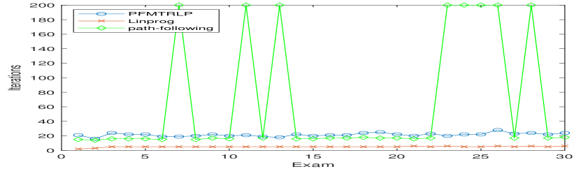
(a) The number of iterations

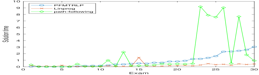
(b) The computational time

Figure 1: The number of iterations and the computational time.

4.2 The rank-deficient problem with noisy data

For a real-world problem, the rank of matrix $A$ in problem (1) may be deficient and the constraints are even inconsistent when the right-hand-side vector $b$ has small noise. However, the constraints of the original problem are intrinsically consistent. In order to evaluate the effect of PFMTRLP handling those problems, we select some rank-deficient problems from the NETLIB collection NETLIB as test problems and compare it with linprog.m for those problems with or without the small noisy data.

The numerical results of the problems without the noisy data are arranged in Table 2. Then, we set $b=b+\text{rand}(m,\,1)*\epsilon$ for those test problems, where $\epsilon=10^{-5}$. The numerical results of the problems with the small noise are arranged in Table 3. From Tables 2 and 3, we can find that PFMTRLP can solve all those problems with or without the small noise. However, from Table 3, we find that linprog.m can not solve some problems with the small noise since inprog.m outputs $NaN$ for those problems. Furthermore, although linprog.m can solve some problems, the KKT errors or the primal-dual gaps are large. For those problems, we conclude that linprog.m also fails to solve them. Therefore, from Table 3, we find that PFMTRLP is more robust than linprog.m for the rank-deficient problem with the small noisy data.

Table 2: Numerical results of some rank-deficient problems from NETLIB.

Problem ($m\times n$, $r$)	PFMTRLP				linprog
	KKTError	Gap	Iter	CPU	KKTError	Gap	Iter	CPU
lp_brandy ($220\times 303$, 193)	2.37E-03	3.57E-02	38	0.19	2.44E-08	1.14E-08	16	0.09
lp_bore3d ($233\times 334$, 231)	3.00E-08	3.32E-06	43	0.22	5.67E-10	1.37E+03	17	0.24
lp_wood1p ($244\times 2595$, 243)	5.09E-05	3.09E-05	100	5.28	1.80E-12	3.16E-11	20	0.26
lp_scorpion ($388\times 466$, 358)	6.16E-07	8.65E-05	37	0.64	2.12E-13	5.08E-08	14	0.05
lp_ship04s ($402\times 1506$, 360)	7.06E-07	2.71E-03	36	1.83	2.39E-07	2.24E-04	13	0.03
lp_ship04l ($402\times 2166$, 360)	1.79E-07	1.00E-03	36	2.48	1.04E-11	1.02E-04	12	0.08
lp_degen2 ($444\times 757$, 442)	8.90E-07	4.45E-05	35	1.23	2.79E-13	9.43E-10	14	0.40
lp_bnl1 ($643\times 1586$, 642)	7.40E-07	6.50E-04	97	11.33	3.36E-09	3.16E-06	26	0.08
lp_ship08s ($778\times 2467$, 712)	4.34E-07	3.29E-03	41	12.72	2.12E-11	1.98E-07	14	0.04
lp_qap8 ($912\times 1632$, 742)	6.84E-07	1.82E-04	22	4.78	2.67E-11	6.48E-07	9	0.49
lp_25fv47 ($821\times 1876$, 820)	5.74E-07	9.20E-04	80	14.67	3.35E-10	6.10E-11	25	0.24
lp_ship08l ($778\times 4363$, 712)	9.95E-07	9.87E-03	40	18.84	1.07E-09	4.28E-03	15	0.15
lp_ship12l ($1151\times 5533$, 1041)	9.22E-07	4.21E-03	47	37.06	4.08E-10	1.15E-02	15	0.06
lp_ship12s ($1151\times 2869$, 1042)	3.01E-07	9.36E-04	47	26.11	1.75E-11	1.50E-05	16	0.05
lp_degen3 ($1503\times 2604$, 1501)	4.79E-07	1.01E-05	48	27.61	5.90E-10	3.55E-08	21	0.52
lp_qap12 ($3192\times 8856$, 2794)	7.00E-07	6.86E-04	25	228.75	1.01E-05	2.95E-04	85	218.06
lp_cre_c ($3068\times 6411$, 2981)	7.97E-07	4.79E-01	90	516.67	5.15E-10	4.50E-02	27	0.21
lp_cre_a ($3516\times 7248$, 3423)	7.86E-07	7.02E-01	83	707.98	7.26E-09	7.10E-02	28	0.24

Table 3: Numerical results of rank-deficient problems with noise $\epsilon=10^{-5}$.

Problem ($m\times n$, $r$)	PFMTRLP				linprog
	KKTError	Gap	Iter	CPU	KKTError	Gap	Iter	CPU
lp_brandy ($220\times 303$, 193)	4.21E-02	2.63E+00	28	0.06	Failed	Failed	0	0.01
lp_bore3d ($233\times 334$, 231)	1.84E-01	1.69E+01	42	0.19	Failed	Failed	0	0.01
lp_scorpion ($388\times 466$, 358)	5.03E-02	1.05E+01	18	0.36	Failed	Failed	0	0.01
lp_degen2 ($444\times 757$, 442)	1.41E-03	9.63E-02	28	1.22	2.92E-04	2.12E+10	52	0.37
lp_ship04s ($402\times 1506$, 360)	3.91E-02	2.93E+02	23	1.56	Failed	Failed	0	0.00
lp_bnl1 ($643\times 1586$, 642)	3.49E-03	2.68E+00	61	7.70	Failed	Failed	0	0.01
lp_qap8 ($912\times 1632$, 742)	8.08E-07	2.19E-04	22	4.58	6.24E-04	6.93E+02	6	0.35
lp_25fv47 ($821\times 1876$, 820)	6.34E-07	1.01E-03	80	14.41	Failed	Failed	0	0.01
lp_ship04l ($402\times 2166$, 360)	9.44E-03	7.35E+01	25	2.03	Failed	Failed	0	0.00
lp_ship08s ($778\times 2467$, 712)	1.69E-02	1.72E+02	24	8.31	Failed	Failed	0	0.00
lp_wood1p ($244\times 2595$, 243)	8.91E-04	6.99E-04	60	3.16	2.41E-04	4.64E+07	33	0.62
lp_degen3 ($1503\times 2604$, 1501)	9.56E-04	2.92E-02	37	24.06	6.84E-04	1.89E+05	77	2.53
lp_ship12s ($1151\times 2869$, 1042)	1.36E-02	6.26E+01	31	18.39	Failed	Failed	0	0.03
lp_ship08l ($778\times 4363$, 712)	1.36E-02	1.55E+02	24	12.80	Failed	Failed	0	0.00
lp_ship12l ($1151\times 5533$, 1041)	1.18E-02	5.88E+01	31	29.44	Failed	Failed	0	0.00
lp_cre_c ($3068\times 6411$, 2981)	5.81E-02	3.84E+04	43	277.59	Failed	Failed	0	0.01
lp_cre_a ($3516\times 7248$, 3423)	7.37E-02	6.73E+04	37	350.22	Failed	Failed	0	0.00
lp_qap12 ($3192\times 8856$, 2794)	7.01E-07	6.86E-04	25	240.84	2.07E-02	1.40E+03	10	24.80

5 Conclusions

For the rank-deficient linear programming problem, we give a preprocessing method based on the QR decomposition with column pivoting. Then, we consider the primal-dual path-following and the trust-region updating strategy for the postprocessing problem. Finally, we prove that the global convergence of the new method when the initial point is strictly prima-dual feasible. According to our numerical experiments, the new method (PFMTRLP) is more robust than the path-following methods such as pathfollow.m (p. 210, FMW2007 ) and linprog.m MATLAB ; Mehrotra1992 ; Zhang1998 for the rank-deficient problem with the small noisy data. Therefore, PFMTRLP is worth exploring further as a primal-dual path-following method with the new adaptive step size selection based on the trust-region updating stratgy. The computational efficiency of PFMTRLP has a room to improve.

References

- (1) I. Adler and R.D.C. Monteiro, Limiting behavior of the affine scaling continuous trajectories for linear programming problems, Math. Program. 50 (1991), pp. 29–51.
- (2) E.L. Allgower and K. Georg, Introduction to Numerical Continuation Methods, SIAM, Philadelphia, 2003.
- (3) E.D. Andersen and K.D. Andersen, Presolving in linear programming, Math. Program. 71 (1995), pp. 221–245.
- (4) E.D. Andersen, Finding all linearly dependent rows in large-scale linear programming, Optim. Methods Softw. 6 (1995), pp. 219–227.
- (5) U.M. Ascher and L.R. Petzold, Computer Methods for Ordinary Differential Equations and Differential-Algebraic Equations, SIAM, Philadelphia, 1998.
- (6) I. Averbakh and Y.B. Zhao, Explicit reformulations for robust optimization problems with general uncertainty sets, SIAM J. Optim. 18 (2008), pp. 1436–1466.
- (7) O. Axelsson and S. Sysala, Continuation Newton methods, Computer and Mathematics with Applications 70 (2015), pp. 2621–2637.
- (8) F.H. Branin, Widely convergent method for finding multiple solutions of simultaneous nonlinear equations, IBM J. Res. Dev. 16 (1972), pp. 504–521.
- (9) K.E. Brenan, S.L. Campbell, and L.R. Petzold, Numerical solution of initial-value problems in differential-algebraic equations, SIAM, Philadelphia, 1996.
- (10) A. R. Conn, N. Gould, and Ph. L. Toint, Trust-Region Methods, SIAM, 2000.
- (11) M. T. Chu and M. M. Lin, Dynamical system characterization of the central path and its variants- a vevisit, SIAM J. Appl. Dyn. Syst. 10 (2011), pp. 887-905.
- (12) B.D. Craven and S.M.N. Islam, Linear programming with uncertain data: extensions to robust optimization, J. Optim. Theory Appl. 155 (2012), pp. 673–679.
- (13) D.F. Davidenko, On a new method of numerical solution of systems of nonlinear equations (in Russian), Dokl. Akad. Nauk SSSR 88 (1953), pp. 601–602.
- (14) P. Deuflhard, Newton Methods for Nonlinear Problems: Affine Invariance and Adaptive Algorithms, Springer, Berlin, 2004.
- (15) P. Deuflhard, H.J. Pesch, and P. Rentrop, A modified continuation method for the numerical solution of nonlinear two-point boundary value problems by shooting techniques, Numer. Math. 26 (1975), pp. 327–343.
- (16) J.E. Dennis and R. B. Schnabel, Numerical Methods for Unconstrained Optimization and Nonlinear Equations, SIAM, Philadelphia, 1996.
- (17) E.J. Doedel, Lecture notes in numerical analysis of nonlinear equations, in Numerical Continuation Methods for Dynamical Systems, B. Krauskopf, H.M. Osinga, and J. Galán-Vioque, eds., Springer, Berlin, 2007, pp. 1–50.
- (18) M.C. Ferris, O.L. Mangasarian, and S.J. Wright, Linear Programming with MATLAB, SIAM, Philadelphia, 2007. Software available at http://pages.cs.wisc.edu/~ferris/ferris.books.html.
- (19) A.V. Fiacco and G.P. McCormick, Nonlinear programming: Sequential Unconstrained Minimization Techniques, SIAM, Philadelphia, 1990.
- (20) O. Güler and Y. Ye, Convergence behavior of interior-point algorithms, Math. Program. 60 (1993), pp. 215–228.
- (21) C.C. Gonzaga, Path-following methods for linear programming, SIAM Rev. 34 (1992), pp. 167–224.
- (22) G.H. Golub and C.F. Van Loan, Matrix Computation, 4th ed., The John Hopkins University Press, Baltimore, 2013.
- (23) E. Hairer and G. Wanner, Solving Ordinary Differential Equations II, Stiff and Differential-Algebraic Problems, 2nd ed., Springer, Berlin, 1996.
- (24) D.J. Higham, Trust region algorithms and timestep selection, SIAM J. Numer. Anal. 37 (1999), pp. 194–210.
- (25) N. Karmarkar, A new polynomial-time algorithm for linear programming, Combinatorica 4 (1984), pp. 373–395.
- (26) L.-Z. Liao, A study of the dual affine scaling continuous trajectories for linear programming, J. Optim. Theory Appl. 163 (2014), pp. 548–568.
- (27) X.-L. Luo, A second-order pseudo-transient method for steady-state problems, Appl. Math. Comput. 216 (2010), pp. 1752–1762.
- (28) X.-L. Luo, A dynamical method of DAEs for the smallest eigenvalue problem, J. Comput. Sci. 3 (2012), pp. 113–119.
- (29) X.-L. Luo, J.-H. Lv and G. Sun, Continuation method with the trusty time-stepping scheme for linearly constrained optimization with noisy data, Optim. Eng., Accepted, available at http://doi.org/10.1007/s11081-020-09590-z or arXiv preprint http://arxiv.org/abs/2005.05965, December 20, 2020.
- (30) X.-L. Luo, H. Xiao and J.-H. Lv, Continuation Newton methods with the residual trust-region time-stepping scheme for nonlinear equations, arXiv preprint no. 2006.02634 available at https://arxiv.org/abs/2006.02634, June 2020.
- (31) MATLAB 9.6.0 (R2019a), The MathWorks Inc., available at http://www.mathworks.com, 2019.
- (32) S. Mehrotra, On the implementation of a primal-dual interior point method, SIAM J. Optim. 2 (1992), pp. 575–601.
- (33) R.D.C. Monteiro, Convergence and boundary behavior of the projective scaling trajectories for linear programming, Math. Oper. Res. 16 (1991), pp. 842–858.
- (34) Cs. Mészáros and U.H. Suhl, Advanced preprocessing techniques for linear and quadratic programming, OR Spectrum 25 (2003), pp. 575-595.
- (35) The NETLIB collection of linear programming problems, http://www.netlib.org.
- (36) J. Nocedal and S.J. Wright, Numerical Optimization, Springer, Berlin, 1999.
- (37) J.M. Ortega and W.C. Rheinboldt, Iteration Solution of Nonlinear Equations in Several Variables, SIAM, Philadelphia, 2000.
- (38) P.Q. Pan, A fast simplex algorithm for linear programming, J. Comput. Math. 28 (2010), pp. 837–847.
- (39) M.J.D. Powell, Convergence properties of a class of minimization algorithms, in Nonlinear Programming 2, O. L. Mangasarian, R. R. Meyer, and S. M. Robinson, eds., Academic Press, New York, 1975, pp. 1-27.
- (40) L.F. Shampine, I. Gladwell, and S. Thompson, Solving ODEs with MATLAB, Cambridge University Press, Cambridge, 2003.
- (41) K. Tanabe, Continuous Newton-Raphson method for solving an underdetermined system of nonlinear equations, Nonlinear Anal. 3 (1979), pp. 495–503.
- (42) K. Tanabe, Centered Newton method for mathematical programming, in System Modeling and Optimization: Proceedings of the 13th IFIP conference, vol. 113 of Lecture Notes in Control and Information Systems, Springer, Berlin, 1988, pp. 197–206.
- (43) S.J. Wright, Primal-dual Interior Point Methods, SIAM, Philadelphia, 1997.
- (44) Y.Y. Ye, Interior Point Algorithms-Theory and Analysis, Wiley, New York, 1997.
- (45) Y. Ye, M. J. Todd and S. Mizuno, An O()-iteration homogeneous and self-dual linear programming algorithm, Math. Oper. Res. 19 (1994), pp. 53–67.
- (46) Y. Yuan, Recent advances in trust region algorithms, Math. Program. 151: 249-281, 2015.
- (47) Z.-D. Yuan, J.-G. Fei, and D.-G. Liu, The Numerical Solutions for Initial Value Problems of Stiff Ordinary Differential Equations (in Chinese), Science Press, Beijing, 1987.
- (48) Y. Zhang, Solving large-Scale linear programs by interior-point methods under the MATLAB environment, Optim. Methods Softw. 10 (1998), pp. 1–31.
- (49) L.H. Zhang, W.H. Yang, and L.-Z. Liao, On an efficient implemetation of the face algorithm for linear programming, J. Comput. Math. 31 (2013), pp. 335–354.