Line-of-Sight MIMO for High Capacity Millimeter Wave Backhaul in FDD Systems

Abstract

Wireless backhaul is considered to be the key part of the future wireless network with dense small cell traffic and high capacity demand. In this paper, we focus on the design of a high spectral efficiency line-of-sight (LoS) multiple-input multiple-output (MIMO) system for millimeter wave (mmWave) backhaul using dual-polarized frequency division duplex (FDD). High spectral efficiency is very challenging to achieve for the system due to various physical impairments such as phase noise (PHN), timing offset (TO) as well as the poor condition number of the LoS MIMO. In this paper, we propose a holistic solution containing TO compensation, PHN estimation, precoder/decorrelator optimization of the LoS MIMO for wireless backhaul, and the interleaving of each part. We show that the proposed solution has robust performance with end-to-end spectral efficiency of 60 bits/s/Hz for 8x8 MIMO.

I Introduction

Dense small cells and femtocells have been proposed to enhance the spatial reuse and boost the capacity of hot spots in future wireless networks [1, 2]. As a result, future wireless networks may comprise a substantial number of small base stations, and the backhaul transmission will be a critical capacity and cost bottleneck. In this paper, we focus on designing a very high spectral efficiency mmWave backhaul transmission using MIMO technology for future wireless networks.

MIMO has been widely used in 3GPP long term evolution (LTE) and 5G systems as a key technique to enable the capacity requirement of the wireless access network. Leveraging the rich scattering in the non-line-of-sight (NLoS) fading channels, spatial multiplexing for MIMO systems has been widely studied in [3]. However, there are various technical challenges in adopting the MIMO technique for improving the spectral efficiency of the wireless backhaul. First, in the context of wireless backhaul, the propagation channel is primarily LoS due to the high carrier frequency together with the narrow beamwidths being used. With limited scattering in the propagation environment, the LoS MIMO channel responses can be highly correlated, leading to a rank deficient channel matrix. Nevertheless, by optimizing the antenna placements, the capacity and rank of the LoS MIMO channel can be improved with a large separation between the antennas in the arrays [4, 5]. However, it is costly to install arrays with large antenna-separation, especially for MIMO systems. This poses the technical challenge in adopting the MIMO technique for improving the spectral efficiency of the wireless backhaul since low antenna-separation arrays will lead to a poor condition number of the LoS MIMO channel and the spatial multiplexing benefit can be jeopardized.

The second challenge is brought by the existence of physical impairments in the system, such as TO and PHN. The presence of timing offsets among the transmit and receive antenna will bring severe inter-symbol interference (ISI), which will degrade the performance of the wireless backhaul. As a result, this poses a very stringent requirement for accurate timing synchronization. Additionally, PHN in MIMO systems will bring two penalties in the MIMO system, namely the demodulation penalty caused by phase distortion to signal constellation and the multi-access interference (MAI) penalty induced by the coherency loss of the precoder and decorrelator. These physical impairments usually exist in practical wireless backhaul, the effect of which is more severe in mmWave systems [6] due to the high carrier frequency. Unlike wireless access applications, the target spectral efficiency of wireless backhaul is very high. These physical impairments can be the performance bottleneck for wireless backhaul and pose a very stringent requirement for accurate estimation and compensation of the TO and PHN. Unfortunately, the spatial multiplexing in MIMO systems will cause severe MAI, which is a huge hurdle for the compensation of these impairments. Furthermore, dual-polarization is usually adopted in wireless MIMO backhaul [7] to overcome the space limitation, which allows two orthogonal streams from each dipole antenna to travel in the same bandwidth at the same time (one vertically (V mode) and one horizontally (H mode)). In such a dual-polarized system, high cross-polarization discrimination (XPD) of each dipole antenna is required to reduce the interference between cross-polar link transmission. However, high XPD together with severe MAI will lead to inaccurate cross-polar link measurements for the TO and PHN, making it more challenging to estimate and compensate these physical impairments. Thus, a novel and holistic solution considering the physical impairments for mmWave LoS MIMO backhaul with dual-polarization is required.

There are many existing works that considered different subsets of the aforementioned physical impairments [8, 9, 10, 11, 12, 13, 14, 15, 16, 17, 18, 6]. TO estimation has been well studied in [9, 10, 11]. In [9], the authors propose a maximum likelihood (ML) estimator to the TO in the MIMO system with an impractical assumption that the TOs are identical across all the antennas. [10, 11] propose estimation methods of different TOs over antennas. However, there are strict assumptions of TO in these works. Specifically, [10] assumes TOs are small and within one symbol time and [11] only considers TOs that are multiples of symbol time. In addition, these works only estimate the sum-offsets and the preamble used in this work may fail due to the severe MAI induced by the high XPD in the dual-polarized LoS MIMO channel.

PHN estimation algorithms in single-input single-output (SISO) systems are widely studied in [12, 13, 14, 19]. However, these methods cannot be applied to MIMO systems since the received signal at each antenna will be influenced by multiple PHNs in the transmitters, which needs to be jointly estimated. For MIMO systems, PHN estimation and compensation algorithms are proposed in [15, 16, 17] with data-aided and decision-directed sum-PHNs estimators. However, [15] assumes that the channel is perfectly known at the receiver and [16, 17] have ignored the effect of TOs at the transceiver. In addition, the high XPD in dual-polarized MIMO is not considered, hence, the sum-PHNs extracted from the estimated channel will have large estimation errors for transceiver links with a small amplitude (e.g., the cross-polar links). In these works, after estimating the sum-PHNs, the authors design the decorrelator to equalize the aggregated channel and sum-PHN matrix. These compensation schemes impose a heavy computational burden at the receiver since the PHN is varying over time and the decorrelator needs to be updated along with the variations of the PHN. In [6], the authors propose a method to estimate and compensate the per-antenna PHN for MIMO, but they do not track the time-varying PHN and they ignore the interplay with the precoder and decorrelator. Hence, existing works are not applicable when various impairments are considered in mmWave LoS MIMO. The precoder and decorrelator are key components in MIMO systems to achieve high spectral efficiency for wireless backhaul, since they enable stable multi-stream transmissions. There are a lot of existing works on MIMO precoder/decorrelator design [20, 21, 22]. [20] proposes a unified linear transceiver design framework, in which the optimal decorrelator is fixed as the Wiener filter and the design problem can be formulated as convex optimization problems in terms of precoder under different design criteria. In [21, 22], the authors consider the weighted MMSE optimization and propose low complexity algorithms based on alternative optimization. However, in all these works, the physical impairments such as TO and PHN have been ignored. This may be justified for wireless access applications but these physical impairments cannot be ignored for wireless backhaul applications due to the very high target spectral efficiency. Recently, many works have considered the physical impairments issue. Hardware impairments aware (HIA) MIMO transceivers are proposed in [23, 24, 25]. However, the effect of physical impairments is simply modeled as additive Gaussian noise to each antenna, which is an over-simplification of the impairments due to the TO and the PHN in the MIMO systems. In summary, these existing solutions cannot be applied in our case because of very different target spectral efficiency and the practical considerations of the LoS MIMO.

In this paper, we adopt a holistic approach and propose a practical solution for a dual-polarized LoS MIMO in mmWave backhaul addressing the aforementioned physical impairments. The solution is not a trivial combination of existing techniques as each component is inter-related. Based on the proposed solution, we can achieve very high spectral efficiency (e.g., 60 bits/s/Hz with 8x8 MIMO) and fully unleash the potential of the LoS MIMO in mmWave backhaul applications. The following summarizes our contributions.

• Decentralized Spatial Timing Estimation and Compensation: We propose a low complexity spatial timing estimator that has a similar complexity to the cross-correlation approach [8, 11] but it is capable of utilizing spatial information across different antennas to estimate the per-antenna TO. The proposed spatial TO estimator only requires local information and hence it can be implemented separately at the transmitter and receiver. To overcome the strong MAI induced by spatial multiplexing of dual-polarized LoS MIMO channels, we propose new preamble sequences with improved auto-correlation and cross-correlation rejection. Based on this, we propose a decentralized timing compensation scheme where the transmitter and receiver compensate for the TO based only on local information without any explicit signaling.

• Decentralized Phase Noise Estimation and Compensation with Decision Feedback. We propose a low complexity per-antenna PHN estimation and compensation scheme, which enables compensation for both the phase distortion to the received symbols and the MAI caused by the loss of coherence of the precoder and decorrelator due to the drifting of PHN. To reduce the pilot overhead, we adopt the decision feedback and regression-based fusion to enhance the PHN estimation quality. The proposed PHN estimator has low complexity and requires local information only. Based on this, we propose a decentralized PHN compensation scheme, which compensates the per-antenna PHN locally at the transmitter and the receiver.

• Robust MIMO Precoder and Decorrelator Design: We exploit the MIMO precoder and decorrelator to suppress the inter-symbol interference (ISI) and MAI induced by the physical impairments of the TO and the PHN. We show that the precoder and decorrelator can significantly alleviate the requirement of the TO compensation and PHN compensation to achieve very high spectral efficiency for mmWave backhaul applications. The design is formulated as a nonconvex optimization problem. By exploiting structures in the ISI and MAI, we transform the problem into a tractable form and propose a low complexity solution using alternative optimization techniques.

This paper is organized as follows. In Section II, we present the system model, including the mmWave dual-polarized LoS MIMO channel model, the TO model, and the PHN model, as well as the data path in the transmitter and receiver. In Section III, V and IV, the proposed timing synchronization, PHN estimation and compensation, as well as the procoder and decorrelator scheme, respectively, are illustrated. The numerical simulation results and the corresponding discussions are provided in Section VI. Finally, Section VII summarizes the whole work.

Notations: In this paper, lowercase and upper bold face letters stand for column vectors and matrices, respectively. The operations $\left(\cdot\right){}^{T}$ and $\left(\cdot\right)^{H}$ are respectively, the operations of transpose and conjugate transpose. The entry in the $i$-th row and $j$-th column of matrix $\mathbf{A}$ is $\left[\mathbf{A}\right]{}_{i,j}$ while the $n$-th element of vector $\mathbf{a}$ is $a_{n}$. $a^{*}$ represents the complex conjugate of $a$. $\mathbf{I}_{N}$ is the $N\times N$ identity matrix and $\mathbf{1}_{N}$ denotes the all one vector of dimension $N$. The norms $||\cdot||_{2}$, $|\cdot|$ and $||\cdot||_{F}$ are respectively, the $L_{2}$, $L_{1}$ and Frobenius norm. $\odot$ and $\otimes$ represents the Hadamard product and Kronecker product, respectively. $e^{{}^{j\left(\cdot\right)}}$ is an elementwise operator for vector or matrix input. $\mathcal{CN}(\mu,\sigma^{2})$ denotes the Complex Gaussian distribution with mean, $\mu$ and variance $\sigma^{2}$. $\mathrm{diag}\left(\mathbf{a}\right)$ denotes a diagonal matrix whose diagonal elements are filled with elements of vector $\mathbf{a}$, and $\mathrm{vec}\left(\cdot\right)$ is the vectorization operator. Finally, $g(\cdot)*f(\cdot)$ denotes the convolution of $g(\cdot)$ and $f(\cdot)$.

II System Model

In this paper, we consider mmWave MIMO wireless backhaul in a dual-polarized FDD system. Both the transmitter and the receiver comprise an antenna array mounted on a pole with a primarily LoS channel in between. Each of the transmit (and receive) antennas has a local oscillator that is loosely synchronized to a master control unit. The illustration of the system is shown in Fig.1. We shall elaborate on each part of this system below.

II-A LoS MIMO Channel Model

In mmWave backhaul, a terrestrial link usually exists. Therefore, we consider the Rummler model [26] in this work, which is an LoS propagation model with a single NLoS path caused by the terrestrial reflection between two fixed antenna towers. For a single-input-single-output (SISO) system, the impulse response of the Rummler model can be specified as

$$h\left(t\right)=\delta\left(t\right)+\beta e^{j2\pi f_{0}\tau^{d}}\delta\left(t-\tau^{d}\right),$$ (1)

where the first term represents the LoS path and the second term represents the NLoS path, $\tau^{d}$ is the propagation delay associated with the difference in the propagation time between the LoS path and the NLoS path and is assumed to be within one symbol time. $f_{0}$ denotes the notch frequency, which will be anywhere in the spectral efficiency. We consider the minimum-phase case of the Rummler model ($\beta\leq 1$), where we set the channel gains $\beta=1-10^{-\frac{\rho}{20}}$, with $\rho$ denoting the notch depth, which relates the power of the LoS path to that of the NLoS paths.

Generalizing the SISO Rummler model to a dual-polarized $N\times M$ MIMO system, the channel model is given by

$$\tilde{\mathbf{H}}(t) =\mathbf{H}^{LoS}(t)+\mathbf{H}^{NLoS}(t),$$

$$=\mathbf{H}^{LoS}(t)+\mathbf{\bm{\beta}}\odot\mathbf{R}\odot\mathbf{H}^{LoS}(t-\tau^{d})$$ (2)

where $\bm{\beta}$ and $\mathbf{R}$ is the random magnitude attenuation and the random phase rotation matrix, respectively, caused by reflection.Since $\bm{\beta}$ and $\mathbf{R}$ are multiplied element-wisely to the LoS channel response, the expression for the NLoS propagation in (2) can represent any NLoS propagation. The LoS channel $\mathbf{H}^{LoS}(t)$ is highly deterministic [27] and can be modeled as

$$\mathbf{H}^{LoS}=\mathbf{H}_{xp}\otimes\mathbf{J}_{\frac{N}{2}\times\frac{M}{2}}\odot\mathbf{H}_{A},$$ (3)

where $\mathbf{H}_{xp}\in\mathbb{C}^{2\times 2}$ contains the cross-polar gains, $\mathbf{\mathbf{J}}_{\frac{N}{2}\times\frac{M}{2}}$ is the $\frac{N}{2}\times\frac{M}{2}$ all ones matrix and $\mathbf{H}_{A}\in\mathbb{C}^{\text{$N$$\times$$M$}}$ is the array response matrix between transmitter and receiver with $N$ and $M$ flat-panel dual-polarized MIMO antenna arrays. Note that in this paper, we assume spherical curvature of the propagating waves, thus the array response $\mathbf{H}_{A}$ is given by

$$[\mathbf{H}_{A}]_{i,j} =e^{-j\frac{2\pi}{\lambda}d_{i,j}},$$

where $d_{i,j}$ is the distance between the $i$-th receiver antenna and the $j$-th transmit antenna. A similar propagation assumption and the array response matrix can be found in [6], in which the dual-polarized array is not considered.

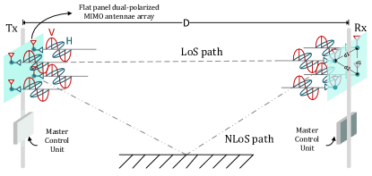
Figure 1: Illustration of antenna arrays and geometry of an $8\times 8$ LoS dual-polarized MIMO system. Flat-panel dual-polarized MIMO antenna arrays are applied with antenna spacing $d1$, $d2$, where $d2=\sqrt{2}d1$. The distance between the transmitter and the receiver is $D$.

With dual-polarized MIMO antennas, XPD of the antennas has a significant influence on the system performance. In general, high antenna XPD is desired to leverage the benefits of dual-polarization [28, 29]. However, high XPD also causes very weak cross-polar transmission links, i.e., the link between the horizontal mode to the vertical mode of each dipole antenna. This will cause a great challenge for the estimation of the TO and PHN since the physical impairments are different on each antenna and the estimation for these physical impairments requires measurements from all the transceiver links. Moreover, the intensity of the MAI will increase as the number of antennas of the MIMO system increases, which will further distort the cross-polar measurements. For example, in an $8\times 8$ MIMO with a typical $\mathrm{XPD}=20$ dB, the power of the MAI will be $26$ dB of the desired signal for a cross-polar link. We show this influence on TO estimation in Fig. 2 with the timing correlation metric in a cross-polar link using the traditional Zadoff–Chu (ZC) sequence. It is observed that as the number of antennas increases, the severe MAI will induce several peaks of similar intensity in the timing correlation metric. As a result, there might be large timing estimation errors due to the false peaks in the metric.

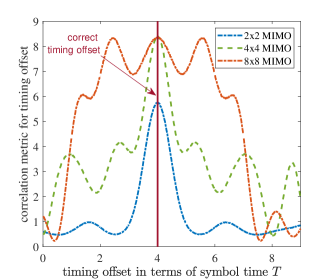
Figure 2: Correlation metric for TO estimation in a cross-polar link for different numbers of antennas. The traditional ZC sequence is used as the preamble sequence for TO estimation. $\mathrm{XPD}$ is set to a typical value of $20$ dB, and the TO is set to be 4 times the symbol time.

II-B Timing offset Model

In mmWave MIMO wireless backhaul, the transmit antennas are not collocated and hence the clock of each transmit antenna/receive antenna is only roughly synchronized to a master clock. Let $\tau_{j}^{tx}=\frac{1}{T}|\text{offset}_{j}^{tx}-\text{offset}_{1}^{tx}|\text{ }$and $\tau_{i}^{rx}=\frac{1}{T}|\text{offset}_{i}^{rx}-\text{offset}_{1}^{tx}|$ denote the normalized TO of the clock at the $j$-th transmit antenna and $i$-th receive antenna, respectively, w.r.t. the symbol duration $T$. Without loss of generality, we assume $\tau_{1}^{rx}=0$ and TOs $\tau_{j}^{tx}$ and $\tau_{i}^{rx}$ are independent quasi-static random processes uniformly distributed in $(0,\tau_{max})$, where $\tau_{max}>1$ is the maximum timing delay that can occur in the system. We denote $\bm{\tau}^{tx}=\left[\tau_{1}^{tx},...,\tau_{M}^{tx}\right]^{T}$ and $\bm{\tau}^{rx}=\left[\tau_{1}^{rx},...,\tau_{N}^{rx}\right]^{T}$ as the TO vector for the transmitter and receiver, respectively, and let $\bm{\tau}=\left[\left(\bm{\tau}^{rx}\right)^{T},\left(\bm{\tau}^{tx}\right)^{T}\right]^{T}$.

II-C Phase Noise Model

In this paper, we consider the independent phase noise $\theta_{j}^{tx}\left(n\right)$ on each transmit antenna and $\theta_{i}^{rx}\left(n\right)$ on each receive antenna. For free-running oscillators, the discrete time PHNs $\theta_{j}^{tx}\left(n\right)$ and $\theta_{i}^{rx}\left(n\right)$ for $j=1,...,M$ and $i=1,...,N$ can be modeled as a Wiener process [31, 15, 16], which are given by

$$\theta_{j}^{tx}\left(n\right) =\theta_{j}^{tx}\left(n-1\right)+\Delta_{j}^{tx}\left(n\right),$$

$$\theta_{i}^{rx}\left(n\right) =\theta_{i}^{rx}\left(n-1\right)+\Delta_{i}^{rx}\left(n\right).$$ (4)

The terms $\Delta_{j}^{tx}\left(n\right)$ and $\Delta_{i}^{rx}\left(n\right)$ are random phase innovations for the oscillators at each sample, assumed to be white real Gaussian processes with $\Delta_{j}^{tx}\left(n\right)\sim\mathcal{N}\left(0,\sigma_{\Delta_{j}^{tx}}^{2}\right)$ and $\Delta_{i}^{rx}\left(n\right)\sim\mathcal{N}\left(0,\sigma_{\Delta_{i}^{rx}}^{2}\right)$, respectively. $\sigma_{\Delta_{j}^{tx}}^{2}$ and $\sigma_{\Delta_{i}^{rx}}^{2}$ stands for the variance of the innovations at the $j$-th and $i$-th transmit and receive antennas, respectively, which are given by [16, 32]

$$\sigma_{\Delta_{j}^{tx}}^{2} =2\pi c_{j}^{tx}T_{s},$$

$$\sigma_{\Delta_{i}^{rx}}^{2} =2\pi c_{i}^{rx}T_{s},$$ (5)

where $c_{j}^{tx}$ and $c_{i}^{rx}$ denote the one-sided 3 dB bandwidth of the Lorentzian spectrum of the oscillators at the $j$-th and $i$-th transmit and receive antennas, respectively, and $T_{s}$ is the sampling time. We assume that $\sigma_{\Delta_{j}^{tx}}^{2}$ and $\sigma_{\Delta_{i}^{rx}}^{2}$ are known at the receiver since they are dependent on the oscillator properties.

II-D Transmit and Receive Data Path

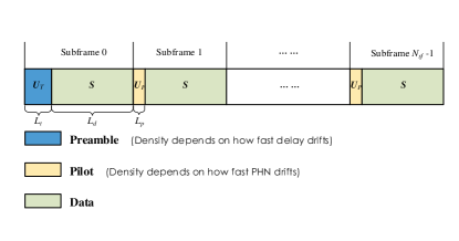
Figure 3: Frame structure for the transmission of preamble, pilot, and data symbols from one transmitter.

We consider a frame structure, illustrated in Fig. 3, in this paper. There is a preamble sequence $\mathbf{U}_{T}=\left[\mathbf{a}_{1},...,\mathbf{a}_{M}\right]^{T}\in\mathbb{C}^{M\times L_{t}}$ with $L_{t}$ symbols at the beginning of each frame for timing synchronization and channel estimation. Specifically, since timing offset is a slowly varying process, we use the preamble of the first frame (initial frame) to perform timing synchronization, while preambles of the rest frames are used for channel estimation. Each frame consists of $N_{sf}$ subframes, and within each subframe, there is a data section with $L_{d}$ symbols, denoted by $\mathbf{S}=\left[\mathbf{s}_{1},...,\mathbf{s_{M}}\right]^{T}\in\mathbb{C}^{M\times L_{d}}$, where $\mathbf{s}_{j}\in\mathbb{C}^{L_{d}\times 1}$ is the transmitted data symbols at $j$-th transmit antenna. In addition, there is a pilot sequence $\mathbf{U}_{P}=\left[\mathbf{b}_{1},...,\mathbf{b}_{M}\right]^{T}\in\mathbb{C}^{M\times L_{p}}$ with length $L_{p}$ at the beginning of each subframe for the estimation and tracking of the PHN over the entire frame. To summarize, the first subframe of each frame has the length of $L_{t}+L_{d}$ symbols, while the other subframes are of length $L_{p}+L_{d}$ symbols. As a result, the overall pilot and preamble overhead is given by $\frac{L_{t}+\left(N_{sf}-1\right)L_{p}}{N_{sf}L_{d}}$. In practice, the period of the preamble is comparable to the coherence time of the channel (which is $10$~$100$ ms for fixed-point wireless backhaul applications [33]). The period of the pilot is more frequent as it has to track the variation of the PHN $\theta_{j}^{tx}\left(n\right)$ and $\theta_{i}^{rx}\left(n\right)$. For a typical oscillator at $f_{c}=28$ GHz, the effective bandwidth of the power spectral density (PSD) of the PHN is $10^{4}$ Hz [34] and hence, the coherence time of the PHN is around $0.1$ ms. Consequently, a pilot density of $100$ pilots per frame would be sufficient. Hence, for a system with a symbol rate of $25$ M/s, the pilot and preamble overhead is around 5% for $L_{t}=256$, $L_{p}=64$, $L_{d}=1280$ and $N_{sf}=100$, which is quite low.

Figure.4 illustrates the uplink and downlink datapath of the transmitter and receiver for the wireless backhaul between two base stations (BSs) A and B. We consider an FDD system, and the transmitter and the receiver of a site share a common oscillator. Hence, the PHN and the TO during downlink for BS A (BS B) as a receiver (transmitter) are identical to the PHN and the TO during uplink for BS A (BS B) as a transmitter (receiver), i.e., in Fig. 4 we have $\theta_{A,j}^{UL}\left(n\right)=\theta_{A,j}^{DL}\left(n\right)$, $\tau_{A,j}^{UL}=\tau_{A,j}^{DL}$, $\forall j$ and $\theta_{B,i}^{UL}\left(n\right)=\theta_{B,i}^{DL}\left(n\right)$, $\tau_{B,i}^{UL}=\tau_{B,i}^{DL}$, $\forall i$. To avoid the abuse of notation, we assume $\theta_{j}^{tx}(n)=\theta_{A,j}^{UL}\left(n\right)$, $\tau_{j}^{tx}=\tau_{A,j}^{UL}$, $\theta_{i}^{rx}(n)=\theta_{B,i}^{UL}\left(n\right)$, $\tau_{i}^{rx}=\tau_{B,i}^{UL}$ in the following illustrations.

Let $g\left(t\right)$ be the response of the pulse-shaping filters evaluated at $t$. The equivalent channel for the $j$-th transmit antenna and the $i$-th receive antenna is given by

$$h_{i,j}^{\mathbf{\bm{\tau}}}\left(t\right)=\left[\tilde{\mathbf{H}}\left(t\right)\right]_{i,j}*g\left(t-\left(\tau_{j}^{tx}+\tau_{i}^{rx}\right)T\right),$$ (6)

where the superscript $\bm{\tau}$ means the variable is parameterized by $\bm{\tau}$. Let $\mathbf{u}_{j}=\left[u_{j}(0),u_{j}(1),...,u_{j}(L-1)\right]^{T}$ denote the complex-valued symbol sequence of length $L$ transmitted by the $j$-th transmitter, which can be a preamble sequence, pilot sequence or data. Suppose the received waveform is sampled at a rate of $Q$ samples per symbol (i.e., $T_{s}=\frac{T}{Q}$), the received signal of $i$-th receive antenna at the $n$-th sample is given by

$$y_{i}\left(n\right)$$ (7)

$$= \sum_{j=1}^{M}\sum_{k=0}^{L-1}e^{j\left[\theta_{j}^{tx}\left(n\right)+\theta_{i}^{rx}\left(n\right)\right]}h_{i,j}^{\mathbf{\tau}}\left(nT_{s}-kT\right)u_{j}\left(k\right)+v_{i}\left(n\right),$$

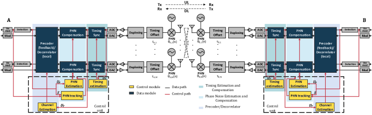
Figure 4: Datapath for the proposed mmWave MIMO backhaul in FDD system.

where $k$ is the symbol index, and $v_{i}\left(n\right)$ is the complex additive white Gaussian noise (AWGN) with zero mean and variance $\sigma^{2}$, i.e., $v_{i}\left(n\right)\sim\mathcal{CN}(0,\sigma^{2}\text{).}$ Specifically, to show a symbol level signal model, the received signal at the $n=kQ$-th sample for symbol index $k=0,...,L-1$ is given by:

$$y_{i}\left(kQ\right) =\underbrace{e^{j\left[\theta_{i}^{tx}\left(kQ\right)+\theta_{i}^{rx}\left(kQ\right)\right]}}_{\mathrm{PHN\ distortion}}\left\{\underbrace{h_{i,i}^{\mathbf{\tau}}\left(0\right)u_{i}\left(k\right)}_{\mathrm{desired\ signal}}\right.$$

$$+\underbrace{\sum_{k^{\prime}=1;k^{\prime}\neq k}^{L-1}h_{i,i}^{\mathbf{\tau}}\left(\left(k-k^{\prime}\right)T\right)u_{i}\left(k^{\prime}\right)}_{\mathrm{ISI}}$$

$$\left.+\underbrace{\sum_{j=1;j\neq i}^{M}\sum_{k^{\prime}=0}^{L-1}h_{i,j}^{\mathbf{\tau}}\left(\left(k-k^{\prime}\right)T\right)u_{j}\left(k^{\prime}\right)}_{MAI}\right\}+\underbrace{v_{i}\left(kQ\right)}_{AWGN}.$$ (8)

From (8), we have the following observations. First, the PHN will introduce a random phase distortion on the received signal constellation during the demodulation process. Furthermore, the MAI and ISI of the spatially multiplexed streams will be mitigated by the precoder and the decorrelator, which are designed based on the estimated channel at the beginning of each frame and remain constant throughout the frame. While the channel will be quasi-static within a frame, the PHN process will be time-varying and hence the PHN distortion will induce loss of coherency of the precoder and decorrelator for symbols within a frame. Second, the impacts of the TO appear in both the ISI and the MAI terms, as illustrated in (8), which will increase both types of interference. These physical impairments may not be a significant performance bottleneck in regular wireless access applications. However, due to the very high spectral efficiency target in wireless backhaul applications, they can be a significant bottleneck.

III Timing Offset Estimation and Compensation

We consider the TO issue in this section. Conventional correlation-based TO estimators correlate the preamble sequences with delayed replicas of the received samples at each receive antenna, and find the maximum correlation peak in the timing metric to estimate the sum-offsets in each transmitter-receiver link. For an $N\times M$ MIMO system, the correlator can estimate $NM$ sum-offsets for all the transmitter-receiver links, but there are only $N+M$ degrees of freedom in these sum-offsets as we only have one unknown TO for each individual antenna to be estimated. Hence, there are correlations among the $NM$ sum-offsets, and this correlation can be further exploited to enable a more accurate TO estimation and compensation for each individual antenna.

Conventionally, the ZC sequence is used as preamble in LTE systems, serving as the primary synchronization signal (PSS) to extract timing information. The cross-correlation of the ZC sequence is low for traditional wireless MIMO applications due to the moderate MAI, thus the accurate estimations of the sum-offsets can be guaranteed. However, the cross-correlation of the ZC sequence is not sufficiently low to mitigate the MAI for a dual-polarized LoS MIMO channel with high XPD, especially for the cross-polar links, which experience severe MAI. Thus, the traditional ZC preamble is not enough to isolate MAI in cross-correlation, which hinders correlator-based timing synchronization from fully utilizing the spatial information. In addition, the high spectral efficiency of wireless backhaul poses a very stringent requirement for accurate timing synchronization, thus preamble sequences with a good auto-correlation property that is robust to ISI are also required. This motivates us to design preamble sequences with superior auto/cross-correlation properties for the TO estimation.

III-A Preamble Sequence Design

Let $\mathbf{a}_{j}=\left[a_{j}\left(0\right),...,a_{j}\left(L_{t}-1\right)\right]^{T}$ denote the preamble sequence transmitted by the $j$-th transmit antenna. The cross-correlation of two preamble sequences $\mathbf{a}_{j}$ and $\mathbf{a}_{j^{\prime}}$ is defined as

$$\eta_{j,j^{\prime}}\left(l\right) =\sum_{k=0}^{L_{t}-1-l}a_{j}\left(k+l\right)a_{j^{\prime}}^{*}\left(k\right)=\eta_{j^{\prime},j}^{*}\left(-l\right),$$

$$\forall l=0,...,L_{t}-1,$$ (9)

where $l$ represents the $l$-th lag. Note that (9) reduces to the auto-correlation of $\mathbf{a}_{j}$ when $j=j^{\prime}$. A satisfying set of preamble sequences should have a very low cross-correlation for all possible lags and a high auto-correlation only when $l=0$, thus, the correlation peak occurs only when the two sequences are from the same antenna and are perfectly aligned. However, [35] shows that it is impossible to design such a set. Fortunately, it is feasible to achieve the required properties in a specific lag interval. Since the TO will not exceed a maximum value of $\tau_{\mathrm{max}}$ in each transmit and receive antenna, we can seek preamble sequences with the required properties at the lag interval $0\leq l\leq\lceil 2\tau_{\mathrm{max}}\rceil$. Such a set of sequences can be obtained by solving the following optimization problems [36]:

$$\mathrm{min}_{\mathbf{U}_{T}} \sum_{j=1}^{M}\sum_{j^{\prime}=1}^{M}\sum_{l=1-L_{t}}^{L_{t}-1}\omega_{l_{f}}\left|\eta_{j,j^{\prime}}\left(l\right)\right|^{2}-\omega_{0}L_{t}^{2}M$$

$$\mathrm{s.t.} \left|a_{j}\left(k\right)\right|=1,\ \ k=0,...,L_{t}-1,\ \ j=1,...,M,$$ (10)

where $\omega_{l}=\omega_{-l}\geq 0$, $l=0,...,L_{t}-1$ are non-negative weights assigned to different time lags and are defined in our problem as

$$\omega_{\pm l}=\left\{\begin{array}[]{cc}1,&0\leq l\leq\lceil 2\tau_{\mathrm{max}}\rceil,\\ 0,&\mathrm{otherwise}.\end{array}\right.$$

The unimodular constraint in (10) ensures the symbols in preamble sequences have a constant amplitude. The optimization problem (10) is solved via the majorization-minimization (MM) algorithm and can be implemented efficiently for very long sequences via fast Fourier transform (FFT) [6]. Fig. 5 shows the auto/cross-correlation of the proposed preamble sequence, compared with the ZC and Walsh sequence. It shows that the proposed sequences provide -70 dB isolation from MAI in cross-correlation and -70 dB isolation from ISI in auto-correlation at desired lags, which is sufficient for TO estimation for our channel model with high XPD.

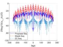
(a) Auto-correlation of $\mathbf{a}_{1}$.

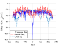
(b) Cross-correlation of $\mathbf{a}_{1}$ and $\mathbf{a}_{2}$.

Figure 5: Auto/cross correlation of the proposed sequence, the ZC sequence, and the Walsh sequence, with $M=8$, $L_{t}=256$ and $\tau_{\mathrm{max}}=5$.

III-B Per-Antenna Timing Offset Estimation

To obtain the per-antenna TO, we first estimate the $NM$ sum-offsets via finding the maximum correlation peak in the timing correlation metric. For a high resolution TO estimation, we consider upsampling at the received signal. Correlating the $Q$-fold upsampled version of the received signal at the $i$-th receive antenna and the preamble from the $j$-th transmit antenna, the timing correlation metric at the $s_{f}$-th sample shift is given by

$$\Lambda_{i,j}\left(s_{f}\right)=\left|\sum_{k=0}^{L_{t}-1}a_{j}^{*}\left(k\right)\cdot y_{i}\left(kQ+s_{f}\right)\right|^{2}.$$

The sum-offset for the $j$-th transmit antenna and the $i$-th receive antenna, $\tau_{i,j}=\tau_{j}^{tx}+\tau_{i}^{rx}$, is obtained by selecting the highest peak in the correlation metric, as given by

$${\hat{\tau}}_{i,j}=\frac{T_{s}}{T}\cdot\left(\arg\max_{s_{f}=0,...,\lceil 2Q\tau_{max}\rceil}\Lambda_{i,j}\left(s_{f}\right)\right).$$

Then, the per-antenna TO $\bm{\tau}=\mathbb{R}^{N+M}$ can be related to the $NM$ sum-offsets by

$$\bm{\gamma}=\bar{\mathbf{I}}_{NM}\bm{\tau},$$ (11)

where $\bm{\gamma}=\left(\tau_{1,1},...,\tau_{1,M},...,\tau_{N,1},...,\tau_{N,M}\right)^{T}\in\mathbb{R}^{NM}$ and $\bar{\mathbf{I}}_{NM}\in\mathbb{R}^{\left(NM\right)\times\left(N+M\right)}$ is given by

$$\bar{\mathbf{I}}_{NM}=\left[\begin{array}[]{cc}\mathbf{I}_{N}\otimes\mathbf{1}_{M}&\mathbf{1}_{N}\otimes\mathbf{I}_{M}\end{array}\right].$$ (12)

The column rank of $\bar{\mathbf{I}}_{NM}$ is only $\left(N+M-1\right)$, thus the transformation (11) is underdetermined and one additional constraint is required. The reference TO, i.e., $\tau_{1}^{rx}=0$ without loss of generality, provides this additional constraint with which the per-antenna TO $\bm{\tau}\in\mathbb{R}^{N+M}$ can be obtained by solving the following LS problem:

$$\hat{\bm{\tau}}= \arg\min_{\mathbf{\tau}}\left\|\bar{\mathbf{I}}_{NM}\bm{\tau}-\hat{\bm{\gamma}}\right\|_{2}$$

$$\ \ \mathrm{s.t.}\ \mathbf{\bm{\tau}}\left(1\right)=0.$$ (13)

III-C Per-Antenna Timing Offset Compensation

In our system, the TOs are compensated with the corresponding transmit and receive pulse shaping filters, specifically, with $g\left(t\right)=g^{tx}\left(t\right)*g^{rx}\left(t\right)$, where $g^{tx}\left(t\right)$ and $g^{rx}\left(t\right)$ represents the transmit and receive pulse shaping filters, respectively. The TOs are compensated using $g^{tx}\left(t+\hat{\tau}_{j}^{tx}\right)$ and $g^{rx}\left(t+\hat{\tau}_{i}^{rx}\right)$ at the $j$-th transmit and $i$-th receive antenna, respectively. Thus, the resulting equivalent channel after TO compensation will be

$$h_{i,j}^{\Delta\bm{\tau}}\left(t\right)=\left[\tilde{\mathbf{H}}\left(t\right)\right]_{i,j}*g\left(t-\left(\Delta\tau_{j}^{tx}+\Delta\tau_{i}^{rx}\right)T\right),$$

where $\Delta\tau_{j}^{tx}=\tau_{j}^{tx}-\hat{\tau}_{j}^{tx}$ and $\Delta\tau_{i}^{rx}=\tau_{i}^{rx}-\hat{\tau}_{i}^{rx}$ represents the residual TO at the $j$-th transmit and $i$-th receive antenna, respectively.

Since the TOs of BS A (BS B) are identical in the downlink and uplink transmission, the TO estimated during downlink (uplink) for BS A (BS B) as a receiver can also be used to compensate the TO during uplink (downlink) for BS A (BS B) as a transmitter. Thus, the per-antenna TO compensation can be implemented by only using the local information in each BS without feedback. For example, consider an FDD system between BS A (with $M$ antennas) and BS B (with $N$ antennas), as illustrated in Fig. 4. The per-antenna TO compensation scheme is described in Fig. 6. The received samples in BS B during uplink transmission are used to correlate with the preamble sequences $\mathbf{U}_{T}$ transmitted by BS A to obtain the uplink sum-offsets $\hat{\bm{\gamma}}_{B}^{UL}$, which is then used to obtain per antenna TO $\hat{\bm{\tau}}^{UL}$ by solving the LS problem with constraint $\mathbf{\bm{\tau}}_{B}\left(1\right)=0$ (13). The TOs of the antennas of BS B are then compensated by the first $N$ elements in $\hat{\bm{\tau}}^{UL}$, i.e., $\hat{\bm{\tau}}_{B}^{UL}$ in the corresponding transmit (receive) pulse shaping filters for the downlink (uplink) transmission. The same compensation procedure is implemented for BS A using downlink measurements.

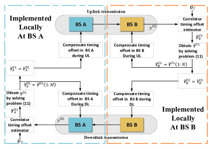
Figure 6: Illustration of the decentralized per-antenna TO compensation.

IV Robust MIMO Precoder and Decorrelator Design

In this section, we propose the precoder/decorrelator design for MAI and ISI suppression. After compensating the TO, there are two physical impairments that will hinder the performance of the precoder/decorrelator. One is the residual of the TO estimation, which is within one symbol time, i.e., $\Delta\mathbf{\tau}_{j}^{tx}\ll T$ and $\Delta\mathbf{\tau}_{i}^{rx}\ll T$, and these residuals will introduce ISI. Another is the PHN, as illustrated in (8), which will introduce MAI. For the convenience of the following discussion, we define $\Delta\bm{\tau}=\left[\left(\Delta\bm{\tau}^{rx}\right)^{T},\left(\Delta\bm{\tau}^{tx}\right)^{T}\right]^{T}=\left[\Delta\tau_{1}^{rx},...,\Delta\tau_{N}^{rx},\Delta\tau_{1}^{tx},...,\Delta\tau_{M}^{tx}\right]^{T}$as the aggregate residual of the TO estimation and the PHN matrix $\big{[}\bm{\Lambda}\left[k\right]\big{]}{}_{i,j}=\theta_{j}^{tx}\left[k\right]+\theta_{i}^{rx}\left[k\right]$ with $\theta_{j}^{tx}\left[k\right]=\theta_{j}^{tx}\left(kQ\right)$ and $\theta_{i}^{rx}\left[k\right]=\theta_{i}^{rx}\left(kQ\right)$, as the PHN of the $k$-th symbol at the $j$-th transmit antenna and the $i$-th receive antenna. Since the operations of downlink and uplink are similar in this section, we omit the indicator for specifying the downlink or the uplink for the channel and the precoder/decorrelator. The channel state information (CSI) is assumed to be static, and the CSI drift caused by the PHN will be discussed in Section V.

IV-A Preliminary for Precoder/decorrelator Design

Before presenting the proposed precoder/decorrelator design, the channel estimation procedure is introduced in this subsection since the CSI is a fundamental preliminary for the precoder/decorrelator design. Due to the existence of the residual of the TO estimation, there is ISI at each symbol transmission. Hence, we need to estimate the CSI for several taps to support the precoder/decorrelator to suppress the ISI. We consider the channels within a finite length window with a $2W+1$ symbol length. Using the discrete expression of the channel (6), the aggregate channel to be estimated is given by

$$\mathbf{\bar{H}}=\left[\mathbf{H}\left[-W\right],...,\mathbf{H}\left[0\right],...,\mathbf{H}\left[W\right]\right]\in\mathbb{C}^{N\times(2W+1)M},$$ (14)

where $\mathbf{H}\left[0\right]\in\mathbb{C}^{N\times M}$ represents the principal channel corresponding to the current transmitted symbol, while $\mathbf{H}\left[w\right]$ is defined as the ISI channel with $w\in\{-W,...,-1,1...,W\}$ corresponding to the adjacent interference symbols. Each subchannel in $\mathbf{\bar{H}}$ is given by

$$[\mathbf{H}\left[w\right]]_{i,j}=h_{i,j}^{\Delta\tau}\left[w\right]e^{j[\bm{\Lambda}\left[k^{*}+w\right]]_{i,j}},\forall w\in\{-W,...,0...,W\},$$ (15)

where $h_{i,j}^{\Delta\tau}\left[w\right]=h_{i,j}^{\Delta\tau}(wT)$. $k^{*}$ is the reference symbol; in other words, we assume the principal channel and ISI channels for each symbol are identical to the principal channel and ISI channels for the $k^{*}$-th symbol. Since the residual of the TO estimation is within one symbol time and the channel is assumed to be static, the input-output relationship at the $k$-th symbol in the preamble for channel estimation can be expressed as

$$\mathbf{y}\left(k\right)=\mathbf{\bar{H}}\mathbf{U}_{T}\left(k\right)+\mathbf{\bm{\nu}}\left[k\right]$$ (16)

where $\mathbf{U}_{T}\left(k\right)=\left[\mathbf{a}\left(k+W\right)^{T},...,\mathbf{a}\left(k\right)^{T},...,\mathbf{a}\left(k-W\right)^{T}\right]^{T}\in\mathbb{C}^{(2W+1)M\times 1}$ is the reshaped preamble for channel estimation and $\bm{\mathbf{\mathbf{\nu}}}\left[k\right]=\bm{\mathbf{\mathbf{\nu}}}\left(kQ\right)$ is the AWGN vector at the $k$-th symbol with variance $\sigma$. Using $L_{t}$ preamble symbols at the beginning of each frame (except the initial frame for timing) to estimate the CSI, the received signal $\mathbf{Y}\in\mathbb{R}^{N\times L_{t}}$ is given by

$$\mathbf{Y} =\mathbf{\bar{H}}\left[\mathbf{U}_{T}(0),\ldots\mathbf{U}_{T}(L_{t}-1)\right]+\left[\bm{\nu}\left[0\right],\ldots,\bm{\nu}\left[L_{t}-1\right]\right]$$

$$=\mathbf{\bar{H}}\bar{\mathbf{U}}_{T}+\bar{\bm{\nu}}.$$

Then, the CSI estimation is obtained by the LS solution

$$\hat{\bar{\mathbf{H}}}=\underset{\mathbf{\bar{H}}\in\mathbb{C}^{N\times(2W+1)M}}{\mathrm{argmin}}\left\|\mathbf{Y}-\mathbf{\bar{H}}\mathbf{U}_{T}\right\|_{F}^{2}=\mathbf{Y}\mathbf{U}_{T}{}^{H}\left(\mathbf{U}_{T}\mathbf{U}_{T}^{H}\right)^{-1},$$ (17)

where $\hat{\bar{\mathbf{H}}}=\left[\mathbf{\hat{H}}\left[-W\right],...,\mathbf{\hat{H}}\left[0\right],...,\mathbf{\hat{H}}\left[W\right]\right]\in\mathbb{C}^{N\times(2W+1)M}$.

IV-B Optimization Problem Formulation for Precoder/decorrelator Design

We use the estimated CSI to optimize the precoder/decorrelator. Consider a MIMO system, which can support $N_{s}=min\{N,M\}$ parallel transmission streams. In order to suppress MAI and ISI, we apply a memoryless precoder, $\mathbf{F}$$\in\mathbb{C}^{M\times N_{s}}$, at the transmitter, and a memory decorrelator, $\mathbf{\tilde{W}}$=[$\mathbf{W}(-D)^{H},...\mathbf{W}(D)^{H}]^{H}$$\in\mathbb{C}^{N(2D+1)\times N_{s}}$, at the receiver, where $\mathbf{W}(d)\in\mathbb{C}^{N\times N_{s}}$ is the decorrelator at the $d$-th tap. The received signal in the $k$-th symbol time at the $m$-th stream can be represented as

$$r_{m}(k)=\mathbf{\tilde{w}}_{m}^{H}\sum_{\begin{subarray}{c}w^{\prime}=-(D+W)\end{subarray}}^{(D+W)}\mathbf{\tilde{H}}\left[w^{\prime}\right]\mathbf{F}\mathbf{s}(k+w^{\prime})+\mathbf{\tilde{w}}_{m}^{H}\tilde{\bm{\nu}}\left[k\right],$$ (18)

where $\mathbf{\tilde{w}}_{m}$ is the $m$-th column of $\mathbf{\tilde{W}}$, and $\mathbf{\tilde{H}}\left[w^{\prime}\right]=\left[\begin{array}[]{c}\mathbf{\hat{H}}(w^{\prime}+D)\\ \vdots\\ \mathbf{\hat{H}}(w^{\prime}-D)\end{array}\right]$, $\mathbf{\tilde{\bm{\nu}}}\left[w^{\prime}\right]=\left[\begin{array}[]{c}\mathbf{\text{$\bm{\nu}$}}(w^{\prime}+D)\\ \vdots\\ \mathbf{\mathbf{\text{$\bm{\nu}$}}}(w^{\prime}-D)\end{array}\right]$ is the aggregate channel and noise, respectively, after considering the memory effect at the decorrelator. $\mathbf{s}(k)=[s_{1}(k),\ldots s_{N_{s}}(k)]$ is the transmitted symbol vector at the $k$-th symbol time in the data section, and we assume $s_{j}(k)$ $\forall j$ and $\forall k$ are i.i.d with zero mean unit and variance.

The existence of both ISI and MAI in Eq.(18) cannot be handled by traditional solutions, such as singular value decomposition (SVD) or naive water filling due to the existence of both ISI and MAI. Furthermore, considering the practical maximum modulation level constraint (e.g., we assume that the maximum modulation level that can be supported in implementation is 4096-QAM), the design of an optimal precoder/decorrelator is challenging. To achieve a high spectrum efficiency and incorporate ISI, MAI, and the modulation constraint, we formulate the following max-sum-rate problem:

$$\underset{\mathbf{F},\mathbf{\mathbf{\tilde{W}}}}{{\mathrm{maximize}}}\quad\sum\limits_{m=1}^{N_{s}}\min\{\log_{2}(1+\text{SINR}_{m}),\text{$\varpi$}\}$$

$$s.t\quad Tr(\mathbf{F^{H}F})\leq P,$$ (19)

where $\varpi$ is the capacity under a given QAM modulation level, $Q_{M}$, with a small error (e.g., symbol error rate (SER) $<10^{-3}$). $P$ is the total transmit power, and $\text{SINR}_{m}$ is the signal to interference plus noise ratio (SINR) of the $m$-th stream, which can be expressed as

$$\text{SINR}_{m} =\frac{\mathbf{\tilde{w}}_{m}^{H}\mathbf{\mathbf{\tilde{H}}}\left[0\right]\mathbf{f}_{m}\mathbf{f}_{m}^{H}\mathbf{\mathbf{\tilde{H}}}\left[0\right]^{H}\mathbf{\mathbf{\tilde{w}}}_{m}}{\sum_{\begin{subarray}{c}m^{\prime}\neq m\end{subarray}}^{N_{s}}\mathbf{\mathbf{\tilde{w}}}_{m}^{H}\mathbf{\mathbf{\tilde{H}}}\left[0\right]\mathbf{f}_{m^{\prime}}\mathbf{f}_{m^{\prime}}^{H}\mathbf{\mathbf{\tilde{H}}}\left[0\right]\mathbf{\mathbf{\tilde{w}}}_{m}+\sum_{\begin{subarray}{c}w^{\prime}=-(D+W);w^{\prime}\neq 0\end{subarray}}^{(D+W)}\mathbf{\tilde{w}}_{m}^{H}\mathbf{\tilde{H}}\left[w^{\prime}\right]\mathbf{F}\mathbf{F}^{H}\mathbf{\mathbf{\tilde{H}}}\left[w^{\prime}\right]^{H}\mathbf{\mathbf{\tilde{w}}}_{m}+\sigma^{2}\mathbf{\mathbf{\tilde{w}}}_{m}^{H}\mathbf{\mathbf{\tilde{w}}}_{m}}.$$ (20)

IV-C Precoder/decorrelator Design via Alternative Optimization

Problem (19) is non-convex and non-smooth, hence is very challenging to solve. Inspired by [22], we introduce an auxiliary variable $\bm{\Gamma}\in\mathbb{C}^{N_{s}\times N_{s}}$ and use an alternative optimization scheme to find a simple solution to problem (19). Using the variable $\bm{\Gamma}$, problem (19) can be well approximated by

$$\underset{\mathbf{F},\mathbf{\mathbf{\tilde{W}}},\bm{\Gamma}}{{\mathrm{minimize}}}\quad Tr\big{(}\bm{\Gamma}\sum\limits_{m=1}^{N_{s}}\mathbf{I}_{m}^{T}\mathbf{E}(\mathbf{W},\mathbf{F})\mathbf{I}_{m}\big{)}-\log\det(\bm{\Gamma})$$

$$s.t\quad Tr(\mathbf{F^{H}F})\leq P,$$ (21)

$$\quad\quad[\bm{\Gamma}]_{m,m}\leq 2^{\text{$\varpi$}},\forall m,$$

where $\mathbf{I}_{m}$ is the diagonal matrix with diagonal elements as the elements in the $m$-th column of the identity matrix, and

$$\mathbf{E}(\mathbf{\mathbf{\tilde{W}}},\mathbf{F}) =(\mathbf{\tilde{W}}^{H}\mathbf{\tilde{H}}\left[0\right]\mathbf{F}-\mathbf{I})(\mathbf{F}^{H}\mathbf{\tilde{H}}\left[0\right]^{H}\mathbf{\tilde{W}}-\mathbf{I})$$

$$+ \mathbf{\tilde{W}}^{H}\big{(}\sum_{\begin{subarray}{c}w^{\prime}=-(D+W);w^{\prime}\neq 0\end{subarray}}^{(D+W)}\mathbf{\mathbf{\tilde{H}}}[w^{\prime}]\mathbf{F}\mathbf{F}{}^{H}\mathbf{\mathbf{\tilde{H}}}[w^{\prime}]^{H}+\sigma^{2}\mathbf{I}\big{)}\mathbf{\mathbf{\tilde{W}}}.$$ (22)

The details of this approximation can be found in Appendix A.

We then present the detailed update rules using the alternative optimization method for problem (21). At the $t_{iter}$-th iteration of the optimization, we alternatively update $\mathbf{\mathbf{\tilde{W}}},$ $\bm{\Gamma}$ and $\mathbf{F}$ by the following 3 steps:

• Step 1: Update $\mathbf{\tilde{W}}^{(t_{iter})}$ given $\bm{\Gamma}^{(t_{iter}-1)}$ and $\mathbf{F}^{(t_{iter}-1)}$ by

  $$\mathbf{\tilde{W}}^{(t_{iter})}=\mathbf{B}^{-1}\mathbf{\mathbf{\tilde{H}}}[0]\mathbf{F}^{(t_{iter}-1)},$$ (23)

  where

  $$\mathbf{B} =\mathbf{\mathbf{\tilde{H}}}[0]\mathbf{F}^{(t_{iter}-1)}(\mathbf{F}^{(t_{iter}-1)}){}^{H}\mathbf{\mathbf{\tilde{H}}}^{H}[0]$$

  $$+\sum_{\begin{subarray}{c}w^{\prime}=-(D+W);w^{\prime}\neq 0\end{subarray}}^{(D+W)}\mathbf{\mathbf{\tilde{H}}}[w^{\prime}]\mathbf{F}^{(t_{iter}-1)}(\mathbf{F}^{(t_{iter}-1)}){}^{H}\mathbf{\mathbf{\tilde{H}}}[w^{\prime}]^{H}$$ (24)

  $$+\sigma^{2}\mathbf{I}\text{.}$$

• Step 2: Update $\bm{\Gamma}^{(t_{iter})}$ given $\mathbf{\tilde{W}}^{(t_{iter})}$ and $\mathbf{F}^{(t_{iter}-1)}$ by

  $$\bm{\Gamma}^{(t_{iter})}=\min\{[\mathbf{E}(\mathbf{\tilde{W}}^{(t_{iter})},\mathbf{F}^{(t_{iter}-1)})]_{m,m}^{-1},2^{\text{$\varpi$}}\}.$$ (25)

• Step 3: Update $\mathbf{F}^{(t_{iter})}$ given $\mathbf{\tilde{W}}^{(t_{iter})}$ and $\bm{\Gamma}^{(t_{iter})}$ by solving
  

  $$\underset{\mathbf{F}}{{\mathrm{minimize}}}\quad Tr\big{(}\bm{\Gamma}^{(t_{iter})}\sum\limits_{m=1}^{N_{s}}\mathbf{I}_{m}^{T}\mathbf{E}(\mathbf{\tilde{W}}^{(t_{iter})},\mathbf{F})\mathbf{I}_{m}\big{)}$$

  $$s.t\quad Tr(\mathbf{F^{H}F})\leq P.$$ (26)

  Problem (26) is convex, which can be efficiently solved by any solver for convex problems, e.g., CVX Matlab package [37].

These 3 update rules are obtained by the property that problem (21) becomes convex in terms of any individual variable in $\mathbf{F},\mathbf{\mathbf{\tilde{W}}},\bm{\Gamma}$ when fixing the other two. This property guarantees the sequence generated by the above alternative optimization converges to a stationary point of problem (21). To summarize, the precoder/decorrelator can be obtained via Algorithm 1.

Algorithm 1 Alternative optimization algorithm for precoder/decorrelator design

1:  Input: Estimated CSI $\hat{\bar{\mathbf{H}}}$, total power $P$ and noise variance $\sigma^{2}.$

2:  Output: $\hat{\mathbf{F}}$,$\hat{\mathbf{W}}$.

3:  Initialize: Construct $\mathbf{\tilde{H}}\left[w^{\prime}\right],w^{\prime}\in\{-(D+W),\ldots,(D+W)\}$ by $\mathbf{\hat{H}}[w]$. $t_{iter}=0$, any$\mathbf{F}^{(0)}$ satisfy the power constraint, $\bm{\Gamma}^{(0)}=diag(2^{\text{$\varpi$}},\ldots 2^{\text{$\varpi$}})$.

4:  while not converge do

5:     $t_{iter}=t_{iter}+1$

6:     Update $\mathbf{\mathbf{\tilde{W}}}^{(t_{iter})}$ according to Eq.(23) and Eq.(24) with $\mathbf{F}^{(t_{iter}-1)}$, $\bm{\Gamma}^{(t_{iter}-1)}$.

7:     Update $\bm{\Gamma}^{(t_{iter})}$ according to Eq.(25) and Eq.(22) with $\mathbf{F}^{(t_{iter}-1)}$, $\mathbf{W}^{(t_{iter})}$.

8:     Update $\mathbf{F}^{(t_{iter})}$ by solving problem (26) with $\mathbf{\mathbf{\tilde{W}}}^{(t_{iter})}$, $\bm{\Gamma}^{(t_{iter})}$ by any solver for convex problems.

9:  end while

10:  $\hat{\mathbf{F}}=\mathbf{F}^{(t_{iter})}$, $\hat{\mathbf{W}}=\mathbf{\mathbf{\tilde{W}}}^{(t_{iter})}$.

V Phase Noise Estimation and Compensation

After the precoder and decorrelator, the MAI and ISI is suppressed to enable high spectral efficiency transmission. However, the phase of the effective channel changes after the channel estimation stage due to the drifting of the PHN, and thus there will be accumulating MAI caused by the coherence loss in the precoder and decorrelator. As a result, the PHN needs to be tracked and compensated in the data transmission stage, which is the main target of this section.

V-A Per-Antenna PHN Estimation based on Pilots

From equation (15) and (16), the channel estimation stage absorbs the initial PHN into the channel phase response. But as the PHN continues to drift, the effect of coherency loss will become dominant and introduce more MAI. To reset the phase error over one frame, we utilize the $N_{sf}-1$ pilots inserted in a frame after the preamble to estimate the PHN increment from the preamble to each subframe. However, the presence of TO error and multipath creates non-negligible ISI, which deteriorates the PHN estimation quality. Though we can accurately estimate the sum-PHN in each ISI channel matrix as in the channel estimation stage, it requires a long pilot sequence to achieve high accuracy, which introduces significant overhead. In this section, we exploit the interference suppression capability of the precoder/decorrelator to improve the estimation accuracy.

Since the PHN varies very slowly within each pilot sequence, we assume that the PHN is constant during pilot sequence transmission in each subframe. We define the accumulated PHN increment from the preamble to the $q$-th subframe as $\phi_{j}^{tx}\left[q\right]=\theta_{j}^{tx}\left[q(L_{d}+L_{p})\right]-\theta_{j}^{tx}\left[k^{*}\right]$ and $\phi_{i}^{rx}\left[q\right]=\theta_{i}^{rx}\left[q(L_{d}+L_{p})\right]-\theta_{i}^{rx}\left[k^{*}\right]$ for the $j$-th transmit antenna and the $i$-th receive antenna, where $k^{*}$ is the reference symbol we picked in the preamble for channel estimation (as elaborated in Eq.(15)). The collection of the accumulated PHN increments at the $q$-th subframe from all $M$ transmit antennas and from all $N$ receive antennas are denoted by $\bm{\phi}^{tx}\left[q\right]\triangleq\left[\phi_{1}^{tx}\left[q\right],...,\phi_{M}^{tx}\left[q\right]\right]^{T}$ and $\bm{\phi}^{rx}\left[q\right]\triangleq\left[\phi_{1}^{rx}\left[q\right],...,\phi_{N}^{rx}\left[q\right]\right]^{T}$. We assume that after the processing by the precoder/decorrelator, the ISI in the pilot transmissions is canceled, hence the received symbols at the $\left(q+1\right)$-th pilot is given by

$$\mathbf{R}\left[q+1\right]$$

$$= \sum_{d=-D}^{D}\mathbf{W}\left[d\right]^{H}\underbrace{\mathbf{D}_{\Delta\bm{\phi}}^{rx}\left[q\right]\mathbf{H}\left[-d\right]\mathbf{D}_{\Delta\bm{\phi}}^{tx}\left[q\right]}_{\mathbf{H}_{q+1}\left[d\right]}\mathbf{F}\mathbf{U}_{P}+\mathbf{V}\left[q+1\right]$$

$$= \sum_{d=-D}^{D}\mathbf{W}\left[d\right]^{H}\mathbf{H}_{q+1}\left[d\right]\mathbf{X}+\mathbf{V}\left[q+1\right],$$

where

• $\mathbf{D}_{\Delta\mathbf{\phi}}^{rx}\left[q\right]\triangleq\mathrm{diag}\left(e^{j\Delta\bm{\phi}^{rx}\left[q\right]}\right)$ is an $M\times M$ diagonal matrix, where $\Delta\bm{\phi}^{rx}\left[q\right]\triangleq\bm{\phi}^{rx}\left[q+1\right]-\hat{\bm{\phi}}^{rx}\left[q\right]$ collects the PHN increments at the receiver;

• $\mathbf{D}_{\Delta\bm{\phi}}^{tx}\left[q\right]\triangleq\mathrm{diag}\left(e^{j\Delta\bm{\phi}^{tx}\left[q\right]}\right)$ is an $N\times N$ diagonal matrix, where $\Delta\bm{\phi}^{tx}\left[q\right]\triangleq\bm{\phi}^{tx}\left[q+1\right]-\hat{\bm{\phi}}^{tx}\left[q\right]$ collects the PHN increments at the transmitter;

• $\mathbf{H}_{q+1}\left[d\right]\triangleq\mathbf{D}_{\Delta\bm{\phi}}^{rx}\left[q\right]\mathbf{H}\left[-d\right]\mathbf{D}_{\Delta\bm{\phi}}^{tx}\left[q\right]$ is the channel corresponding to the desired pilot signal for tap $d$ at the beginning of the $\left(q+1\right)$-th subframe;

• $\mathbf{X}=\mathbf{F}\mathbf{U}_{P}$ denotes the transmitted signal after applying the precoder $\mathbf{F}$ to the pilots $\mathbf{U}_{P}$ and

• $\mathbf{V}\left[q+1\right]\in\mathbb{C}^{N_{s}\times L_{p}}$ contains the AWGN noise.

To estimate of the PHN increments at $\mathbf{R}\left[q+1\right]$, we use first order Taylor expansion $e^{j\Delta\phi}\approx 1+j\Delta\phi$ to approximate $\mathbf{D}_{\Delta\bm{\phi}}^{rx}\left[q\right]$ and $\mathbf{D}_{\Delta\bm{\phi}}^{tx}\left[q\right]$ by $\mathbf{I}+\mathrm{diag}(j\Delta\bm{\phi}^{tx}\left[q\right])$ and $\mathbf{I}+\mathrm{diag}(j\Delta\bm{\phi}^{rx}\left[q\right])$. We also define $\bm{\Omega}_{m}\left(k\right)\in\mathbb{R}^{NM\times NM}$, with $\left[\bm{\Omega}_{m}^{d}\left(k\right)\right]_{i,j}=[\mathbf{W}\left(d\right)^{H}]_{i,m}\mathbf{H}\left[-d\right]_{i,j}\left[\mathbf{X}\right]_{j,k}$. The collection of the PHN increments $\Delta\bm{\phi}\left[q\right]\triangleq\left[\Delta\bm{\phi}^{rx}\left[q\right]^{T},\Delta\bm{\phi}^{tx}\left[q\right]^{T}\right]^{T}\in\mathbb{R}^{M+N}$ can be obtained by solving the following LS problem:

$$\Delta\hat{\bm{\phi}}\left[q\right] =\arg\min_{\Delta\bm{\phi}\left[q\right]}\left\|\bm{\Xi}\Delta\bm{\phi}\left[q\right]-\left(\mathrm{vec}(\mathbf{R}\left[q+1\right])-\bm{\zeta}\right)\right\|_{2}^{2}$$

$$\mathrm{s.t.} \Delta\bm{\phi}_{1}\left[q\right]=0,$$ (27)

where

$$\bm{\Xi} =\left[\bm{\xi}_{1}^{T}\left(1\right),...,\bm{\xi}_{N_{s}}^{T}\left(1\right),\ldots,\bm{\xi}_{1}^{T}\left(L_{p}\right),\ldots,\bm{\xi}_{N_{s}}^{T}\left(L_{p}\right)\right]$$

with

$$\bm{\xi}_{m}^{T}\left(k\right)=\mathbf{1}_{MN\left(2D+1\right)}^{T}\left[\begin{array}[]{c}\mathrm{diag}\left\{\mathrm{vec}\left[j\left(\bm{\Omega}_{m}^{-D}\left(k\right)\right)^{T}\right]\right\}\\ \vdots\\ \mathrm{diag}\left\{\mathrm{vec}\left[j\left(\bm{\Omega}_{m}^{D}\left(k\right)\right)^{T}\right]\right\}\end{array}\right]\bar{\mathbf{I}}_{NM}$$ (28)

$\forall m=1,\ldots N_{s},k=1,\ldots L_{p}$, and we defined $\bm{\zeta}=\Bigg{[}\mathbf{1}_{MN\left(2D+1\right)}^{T}\bm{\eta}_{1}\left(1\right),\ldots,\mathbf{1}_{MN\left(2D+1\right)}^{T}\bm{\eta}_{N_{s}}\left(L_{p}\right)\Bigg{]}^{T}$ with

$$\bm{\eta}_{m}\left(k\right)=\left[\mathrm{vec}\left[\bm{\Omega}_{m}^{-D}\left(k\right)\right]^{T},...,\mathrm{vec}\left[\bm{\Omega}_{m}^{D}\left(k\right)\right]^{T}\right]^{T}$$ (29)

$\forall m=1,\ldots N_{s},k=1,\ldots L_{p}.$ Problem (27) is derived by expanding $\mathbf{R}\left[q+1\right]$ elementwisely, and the detailed derivation can be found in Appendix B.

The PHN at $\left(q+1\right)$-th pilot is then updated by

$$\hat{\bm{\phi}}\left[q+1\right]=\hat{\bm{\phi}}\left[q\right]+\Delta\hat{\bm{\phi}}\left[q\right]\ \mathrm{for}\ q=0,...,N_{sf}-1,$$

where $\hat{\bm{\phi}}\left[0\right]=0$ as we assume PHN at the preamble is absorbed to the channel and is perfectly estimated during the channel estimation stage.

V-B Per-Antenna PHN Compensation

We focus on the per-antenna PHN compensation in this subsection. Traditionally, the PHN information obtained at the receiver is feedback to the transmitter for PHN compensation. However, per-symbol feedback of PHN estimates will incur too much overhead. Fortunately, the transmitter and receiver share the same oscillator in an FDD system so that the PHN is identical in the uplink and downlink at the same site, which enables local compensation of the PHN and avoids the overhead for PHN feedback. Consider the transmission datapath in Fig. 4, the PHN estimated during downlink (uplink) for BS A (BS B) as a receiver can also be used to compensate the PHN during uplink (downlink) for BS A (BS B) as a transmitter. Thus, PHN compensation can be implemented by using local information only without feedback.

However, unlike the TO compensation, where the reference $\tau_{1}$ is usually known a priori, $\Delta\phi\left[q\right]_{1}$ in (27) is not available in advance to both BS A and BS B. Thus, there will be a common PHN error across all the antennas at the receiver. If we directly use the result $\Delta\hat{\bm{\phi}}\left[q\right]$ to compensate the PHN and the common PHN error is identical to the PHN of the first link, i.e., the sum-PHN at the first receive antenna and first transmit antenna. For example, let

$$\Delta\hat{\bm{\phi}}^{UL}\left[q\right]=\left[\left(\Delta\hat{\bm{\phi}}_{B}^{UL}\left[q\right]\right)^{T},\left(\Delta\hat{\bm{\phi}}_{A}^{UL}\left[q\right]\right)^{T}\right]^{T}$$

and

$$\Delta\hat{\bm{\phi}}^{DL}\left[q\right]=\left[\left(\Delta\hat{\bm{\phi}}_{A}^{DL}\left[q\right]\right)^{T},\left(\Delta\hat{\bm{\phi}}_{B}^{DL}\left[q\right]\right)^{T}\right]^{T}$$

be the estimated $\left(M+N\right)$ PHN vector obtained by solving problem (27) in BS B during uplink and BS A during downlink, respectively. When BS A and BS B compensate the PHN using local information $\Delta\hat{\bm{\phi}}_{A}^{DL}\left[q\right]$ and $\Delta\hat{\bm{\phi}}_{B}^{UL}\left[q\right]$ respectively, the common PHN error at BS A and BS B can be calculated locally by $\hat{\phi}_{A,CM}^{DL}\left[q+1\right]=\Delta\hat{\phi}_{A,1}^{DL}\left[q\right]+\Delta\hat{\phi}_{B,1}^{DL}\left[q\right]$ and $\hat{\phi}_{B,CM}^{UL}\left[q+1\right]=\Delta\hat{\phi}_{B,1}^{UL}\left[q\right]+\Delta\hat{\phi}_{A,1}^{UL}\left[q\right]$, where $\Delta\hat{\phi}_{A,i}^{DL}\left[q\right]$ denotes the $i$-th element of $\Delta\hat{\bm{\phi}}_{A}^{DL}\left[q\right]$.

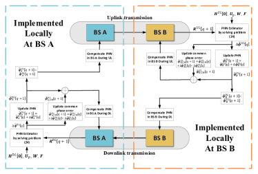
Figure 7: Per-antenna PHN compensation scheme.

The per-antenna PHN compensation scheme is described in Fig. 7. The received symbols $\mathbf{R}^{UL}\left[q+1\right]$ in BS B during uplink transmission are used to compute the estimation for PHN increment $\Delta\hat{\bm{\phi}}^{UL}\left[q\right]$ by solving problem (27), which is then used to obtain per antenna PHN accumulation $\hat{\bm{\phi}}_{B}^{UL}\left[q+1\right]$ and common phase error accumulation $\hat{\phi}_{B,CM}^{UL}\left[q+1\right]$ at BS B. The PHN of the antennas of BS B are then compensated by $\hat{\bm{\phi}}_{B}^{UL}\left[q+1\right]$ in the downlink, while they are compensated by $\hat{\bm{\phi}}_{B}^{UL}\left[q+1\right]+\hat{\phi}_{B,CM}^{UL}\left[q+1\right]$ during the uplink. The same compensation procedure is implemented for BS A using the downlink measurements.

V-C Per-Antenna PHN Tracking based on Decision Feedback

To track the PHN parameter of each antenna in a subframe, we proposed a decision-feedback (DFB) estimator to support PHN estimation during data transmission between consecutive pilots.

The $L_{d}$ symbols in a subframe is split to $N_{b}$ data blocks where each data block contains $L_{b}$ symbols such that $L_{d}=N_{b}L_{b}$. In the practical scenario of interest, the PHN is varying slowly compared to symbol time, the PHNs during each data block are assumed to be constant and we denote the PHN of the $p$-th data block in the $q$-th subframe by $\bm{\phi}^{tx}\left[p;q\right]$ and $\bm{\phi}^{rx}\left[p;q\right]$ for the transmitter and receiver, respectively, and define $\bm{\phi}\left[p;q\right]=\left[\bm{\phi}^{rx}\left[p;q\right]^{T},\bm{\phi}^{tx}\left[p;q\right]^{T}\right]^{T}$. Therefore, in the DFB case, the $L_{b}$ previously detected data symbols $\bar{\mathbf{S}}\left[p;q\right]$ in the $p$-th data block of the $q$-th subframe are used to estimate the PHN parameters $\bm{\phi}\left[p;q\right]$. For simplicity, we assume perfect decision-feedback during data transmission.

Based on the above assumptions, the estimate of PHN increment $\Delta\bm{\phi}\left[p;q\right]=\left[\Delta\bm{\phi}^{rx}\left[p;q\right]^{T},\Delta\bm{\phi}^{tx}\left[p;q\right]^{T}\right]^{T}$ from the $p$-th to the $\left(p+1\right)$-th data block is obtained by solving

$$\Delta\hat{\bm{\phi}}^{DFB}\left[p;q\right] =\arg\min_{\Delta\bm{\phi}}\left\|\mathbf{R}\left[p+1;q\right]-\right.$$

$$\left.\sum_{d=-D}^{D}\mathbf{W}\left(d\right)^{H}\mathbf{D}_{\Delta\bm{\phi}}^{rx}\mathbf{H}\left[-d\right]\mathbf{D}_{\Delta\bm{\phi}}^{tx}\mathbf{F}\bar{\mathbf{X}}\left[p+1;q\right]\right\|^{2},$$ (30)

where $\mathbf{R}\left[p+1;q\right]$ is the received symbols of the $\left(p+1\right)$-th data block in the $q$-th subframe, and $\bar{\mathbf{X}}\left[p+1;q\right]=\mathbf{F}\bar{\mathbf{S}}\left[p+1;q\right]$. The problem can also be approximated by the Taylor expansion on small PHN increments between data blocks and solved using the same technique introduced in pilot PHN estimation as specified in Section V-A. The estimation for accumulated PHN via DFB at the $\left(p+1\right)$-th data block is then updated by

$$\hat{\bm{\phi}}^{DFB}\left[p+1;q\right]=\hat{\bm{\phi}}\left[p;q\right]+\Delta\hat{\bm{\phi}}^{DFB}\left[p;q\right].$$

However, the DFB estimator may be prone to errors in the detection of symbols. Instead, we use moving window averaging to track the evolution of the PHN, i.e., the estimated PHN of $\bm{\phi}\left[p+1;q\right]$ is given by

$$\hat{\bm{\phi}}\left[p+1;q\right]=\left(1-\alpha\right)\hat{\bm{\phi}}\left[p;q\right]+\alpha\hat{\bm{\phi}}^{DFB}\left[p+1;q\right],$$ (31)

where $0\leq\alpha\leq 1$, $p=0,1,...,N_{b}$, and $\hat{\bm{\phi}}\left[0;q\right]=\hat{\bm{\phi}}\left[q\right]$ takes the pilot-aided PHN estimation result. In (31), $\hat{\bm{\phi}}\left[p;q\right]$ is the estimated PHN from the history, while $\hat{\bm{\phi}}^{DFB}\left[p+1;q\right]$ is the new PHN estimate from the DFB in the $\left(p+1\right)$th data block. By adjusting $\alpha$, we strike a balance between the history and the innovation from the DFB.

VI Simulations and Discussions

In this section, the performance of the proposed massive MIMO mmWave backhaul system is evaluated. In the following results, we consider multiple practical cases where $23$ GHz carrier is used and $8\times 8$ flat-panel dual-polarized MIMO antennas arrays are equipped at the transmitter and receiver to transmit data at a distance $D=3$ km, as illustrated in Fig. 1. Within a single the antenna array, antenna element spacing is $d1=\frac{\lambda}{2}$, and the XPD between H mode and V mode in each dual polar element varies from $0$ dB to $30$ dB. All the transmitted signals have been normalized to have unit average power, with symbol duration $T=40$ ns. The propagation delay associated with the interpath is $\tau_{d}=6.3$ ns and the notch depth $\rho$ in the reflected path varies from $10$ dB to $15$ dB. The variance of the AWGN, is set to $\sigma^{2}=\frac{1}{SNR}$ with SNR=$47$ dB. The maximum TOs is $\tau_{max}\cdot T=200\mathrm{ns}$ ($5$ symbols time). The variance of the PHN increment process over one symbol duration is $\sigma_{\Delta}^{2}=10^{-6}$$\mathrm{rad}^{2}$ and we set $\alpha=0.1$ for PHN tracking. The frame structure parameters are chosen as $L_{t}=256$, $L_{p}=64$, $L_{d}=1280$ and $N_{sf}=100$. The number of taps for the ISI channel and the memory decorrelator are respectively, $W=3$ and $D=3$. In the simulation results, we will first demonstrate the efficiency of the proposed methods in each component of this system, i.e., TO estimation and compensation, precoder and decorrelator, PHN estimation and compensation. Finally, we will show the end-to-end simulation results, which incorporate all the components proposed in this work.

VI-A Performance of Individual Design

Figure 8: TO estimation error using the proposed preamble sequence,the ZC sequence, and theWalsh sequence.

Figure. 8 shows the performance comparison of the LS-based TO estimator with the proposed preamble sequence, traditional ZC sequence, and Walsh sequence of same length $L_{t}=256$. The performance metric for TO estimation is the square root of the MSE of the effective sum-offset in each MIMO link, which is defined as $\sqrt{\mathbb{E}\left[\frac{||\bm{\hat{\gamma}}-\bm{\gamma}||_{2}^{2}}{N^{2}}\right]}$, where $\bm{\gamma}$ is the sum-offsets as defined in Section III, and the expectation is taken over 500 realizations. ZC sequence and Walsh sequence act as the baselines to estimate the sum-offsets via the LS-based method. Proposed preamble without LS is another baseline that only adopts the proposed preamble to directly estimate the sum-offsets without the LS procedure in (13). The proposed preamble with LS is the proposed TOs estimation method, in which $\hat{\bm{\gamma}}\in\mathcal{\mathbb{R}}^{N^{2}\times 1}$ is reconstructed from $\hat{\bm{\tau}}\in\mathbb{R}^{2N\times 1}$ by equation (13). As shown in Fig. 8, the proposed method shows superior performance over the other baselines with XPD ranging from $0$ dB to $30$ dB, and the proposed preamble is more robust to higher XPD. The proposed preamble only shows a significant performance decay when XPD $\geq 20$ dB. However, the performance of the ZC sequence and Walsh sequence degrades significantly for XPD $\geq 5$ dB. The LS procedure gives us more than a 2 times higher accuracy in terms of square root MSE for the proposed preamble.

To verify the robustness of the precoder/decorrelator, multiple simulations are performed under different physical impairments. Specifically, the received signal is generated by (8) considering one sample per symbol with $\tau_{max}/T\in(0.001,0.1)$ and $\sigma_{\Delta}\in(0.001,0.1)$. The estimated CSI $\bar{\mathbf{H}}$ required for the precoder/decorrelator is obtained by the channel estimation in subsection IV-A. In the optimization problem for the proposed method, $\varpi$ is set as the capacity under the $4096$-QAM and (SER) $<0.001$. Fig. 9 presents the theoretical sum-rate performance (Eq.(19)) comparisons between the proposed precoder/decorrelator and the SVD solution. The results show that the proposed method outperforms SVD in all the considered scenarios.

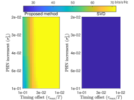
Figure 9: Theoretical sum-rate performance (Eq.(19)) of the proposed method and SVD under different physical impairments, $\rho=10$, SNR=$47$dB, $N=M=8$. A $30\times 30$ grid is constructed for each algorithm with the performance averaged by 100 independent trials at each grid point.

Fig. 10 shows the performance of PHN estimation in pilots over a frame for 100 Monte-Carlo trials. The performance metric is the rooted MSE of the effective sum-PHN in each MIMO link. The accumulated sum-PHNs at $q$-th pilot, denoted as vector $\bm{\vartheta}\left[q\right]$, can also be obtained from the per-antenna PHN $\bm{\phi}\left[q\right]$ via the transformation $\bm{\vartheta}\left[q\right]=\text{$\bar{\mathbf{I}}$}_{NM}\bm{\phi}\left[q\right]$. The baselines extract the PHN by first getting an estimate of the principal channel during the $q$-th pilot transmission $\hat{\mathbf{H}}_{q}\left[0\right]$, then $\bm{\vartheta}\left[q\right]$ is estimated by [6]

$$\hat{\bm{\vartheta}}\left[q\right]=\angle\mathrm{vec}\left(\hat{\mathbf{H}}_{q}\left[0\right]\right)-\angle\mathrm{vec}\left(\hat{\mathbf{H}}\left[0\right]\right).$$ (32)

In getting the principal channel, the first baseline ignores the ISI and uses an LS algorithm [16][6] $\hat{\mathbf{H}}_{q}\left[0\right]=\mathbf{Y}\left[q\right]\mathbf{X}^{H}\left(\mathbf{X}\mathbf{X}^{H}\right)^{-1}$ to directly estimate the principal channel, while the second baseline uses the pilots to estimate the principal and ISI channels with the LS-based channel estimation method introduced in Section IV-A, and then extracts the desired principal channel $\hat{\mathbf{H}}_{q}\left[0\right]$. As observed from Fig. 10, for 0 dB ¡ XPD ¡ 20 dB, the proposed PHN estimation method reaches an estimation error at about 0.002 rad, while the errors of the two $baselines$ increase rapidly to 0.01 rad as XPD increases. This is because, with higher XPD, the phase of cross-polar links is more sensitive to the MAI and noises due to small channel power in these links. It is noted that at low XPD (around 0dB), the proposed PHN estimation method still outperforms the baselines because it leverages the ISI suppression capability of the precoder and decorrelator. The performance of the proposed PHN estimation method starts to decay for high XPD ($>20$ dB) due to loss of measurements in the cross-polar links, but it still outperforms the baselines.

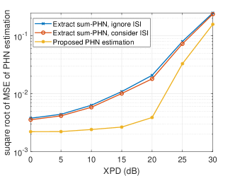
Figure 10: PHN estimation error in pilots over a frame.

VI-B End-to-End Performance

For the end-to-end performance evaluation, we perform 200 Monte-Carlo trials (i.e., independent frames) with XPD $=20$ dB and $\rho=10$ dB in which our proposed holistic method is compared to several baselines. These baselines partially adopt different techniques in the system:

• Baseline 1 [6]: This baseline first estimates the accumulated sum-PHN $\hat{\bm{\vartheta}}\left[q\right]$ by (32). Then, the sum-PHN is converted back to the original transmitter and receiver PHN $\hat{\bm{\phi}}\left[q\right]$ using the pseudo-inverse of $\text{$\mathbf{A}$}_{NM}$. Based on the information of $\hat{\bm{\phi}}\left[q\right]$, PHN de-rotation operations at both the receiver and the transmitter are applied before and after an equalizer to compensate per antenna PHN. The equalizer is calculated based on the principal channel estimated from the received preamble to suppress the MAI. Finally, an MMSE-FIR filter per stream is performed to suppress the ISI.

• Baseline 2 [16]: This baseline extracts accumulated sum-PHN $\bm{\vartheta}\left[q\right]$ in the estimated channel matrix during pilot transmission by (32). This sum-PHN is then combined with the principal channel matrix estimated during the preamble transmission. An MMSE linear decorrelator is constructed based on the combined channel to equalize the effect of the PHN and channel gain. However, since this method pays no attention to the coherence loss effect and the ISI, thus it shows an inferior performance.

• Baseline 3 (SVD): This baseline uses the unitary matrices of the SVD on the estimated principal channel as the precoder and decorrelator. Because this method ignores the ISI and MAI, thus it suffers a poor performance in our considered scenario.

In this experiment, channel coding is not considered and all the approaches adopt the same timing synchronization. To perform an end-to-end experiment and show reasonable results, we take an adaptive modulation strategy by estimating the SINR via Eq. 20 before data transmission. After the precoder/decorrelator calculation, modulation levels according to the estimated SINR are suggested according to the relationship between the modulation level, SINR, and SER where we fix SER $<0.001$ for each stream. Then, the data is transmitted with the Gray mapped $Q_{M}$-QAM symbol where $Q_{M}$ is the suggested modulation level and is demodulated with the hard decision. Note that practical adaptive modulation may not be operated in this way, but taking this strategy will not influence the performance comparisons.

To verify the superiority of the proposed scheme, we first show per stream SINR to verify the reliability and efficiency of the system in a detailed view. Specifically, for the $m$-th stream, $\text{SINR}_{m}(dB)=10\log_{10}\mathbb{E}_{k}\left[\frac{||\mathbf{w}_{m}^{H}\left(e^{j\mathrm{diag}\left(\Delta\bm{\phi}^{rx}\left[k\right]\right)}\mathbf{H}\left[0\right]e^{j\mathrm{diag}\left(\Delta\bm{\phi}^{tx}\left[k\right]\right)}\right)\mathbf{s}\left(k\right)||_{2}^{2}}{||r_{m}(b)-\mathbf{w}_{m}^{H}\left(e^{j\mathrm{diag}\left(\Delta\bm{\phi}^{rx}\left[k\right]\right)}\mathbf{H}\left[0\right]e^{j\mathrm{diag}\left(\Delta\bm{\phi}^{tx}\left[k\right]\right)}\right)\mathbf{s}\left(k\right)||_{2}^{2}}\right]$. In Fig. 11, per stream SINR performance is given among different methods. The highest QAM modulation level that can be achieved by the proposed method at each stream is also given. It is obvious that the proposed method outperforms the baselines of each stream with an over 10 dB gain, and the modulation level achieved by the proposed method can not be afforded by baselines.

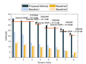
Figure 11: Per-stream SINR performance in the End-to-End experiment.

To show an overall performance, we then compare the BER and Spectrum Efficiency in Table. I. Note that both results are averaged over uplink and downlink effective transmissions.

TABLE I: End-to-End BER and Spectrum Efficiency performance.

	BER($10^{-3}$)	Spectrum Efficiency
		(bits/s/Hz)
Proposed	0.2221	60
Baseline 1	0.6740	15
Baseline 2	0.2036	8
Baseline 3	0.4401	8

From Table. I, the results show that the proposed method can achieve an over $4$ times spectrum efficiency gain compare to all the baselines with a nearly identical BER.

VII Conclusion

This paper proposes a holistic solution to achieve high spectral efficiency for an LoS MIMO system equipped with dual-polarized antenna arrays for wireless backhaul using FDD. Various physical impairments such as TOs and phase noises as well as the effect of multipath are taken into account. An LS-based TO estimator is proposed with a new set of preamble sequences to perform timing synchronization. After channel estimation, an optimization-driven precoder/decorrelator design is proposed to suppress the MAI and ISI introduced by the multipath to maximize the theoretical sum-rate. Additionally, a PHN estimation, tracking, and compensation scheme is proposed to tackle the problem of the coherence loss of precoder/decorrelator due to the drifting of the PHN over a frame. With a simulation setup in a $8\times 8$ LoS MIMO demonstrator, the proposed method can achieve high spectral efficiency at 60 bits/s/Hz. Simulation results also show that our proposed solution outperforms the existing baselines.

Appendix A Derivation of problem (21)

The derivation is similar to [22, Appendix A], except for the procedure used to approximate the non-smoothness in the original problem (19). First, when fixing the other variables, the optimal decorrelator, $\mathbf{\tilde{W}}$ is the MMSE decorrelator as shown in (23). Second, to update the auxiliary variable $\bm{\Gamma}\in\mathbb{C}^{N_{s}\times N_{s}}$, we first check the first-order optimality of $\bm{\Gamma}$ and then do the projection by considering the box constraint for it. The optimal $\bm{\Gamma}$ is a diagonal matrix with $\bm{\Gamma}_{m,m}=\min\{[\mathbf{E}(\mathbf{\tilde{W}},\mathbf{F})]_{m,m}^{-1},2^{\text{$\varpi$}}\}$. Substituting the optimal $\mathbf{\tilde{W}}$ and $\bm{\Gamma}$ into (19) we have

$$\underset{\mathbf{F}}{{\mathrm{maximize}}}\quad -\sum\limits_{m=1}^{N_{s}}\min\{[\mathbf{E}(\mathbf{\tilde{W}}(\mathbf{F}),\mathbf{F})]_{m,m}^{-1},2^{\text{$\varpi$}}\}[\mathbf{E}(\mathbf{\tilde{W}}(\mathbf{F}),\mathbf{F})]_{m,m}$$

$$+\sum\limits_{m=1}^{N_{s}}\min\{\log(1+\text{SINR}_{m}),2^{\text{$\varpi$}}\}$$

$$s.t\quad Tr(\mathbf{F^{H}F})\leq P,$$

where $-\sum\limits_{m=1}^{N_{s}}\min\{[\mathbf{E}(\mathbf{\tilde{W}}(\mathbf{F}),\mathbf{F})]_{m,m}^{-1},2^{\text{$\varpi$}}\}[\mathbf{E}(\mathbf{\tilde{W}}(\mathbf{F}),\mathbf{F})]_{m,m}$ is a constant when $\min\{[\mathbf{E}(\mathbf{\tilde{W}}(\mathbf{F}),\mathbf{F})]_{m,m}^{-1},2^{\text{$\varpi$}}\}=[\mathbf{E}(\mathbf{\tilde{W}}(\mathbf{F}),\mathbf{F})]_{m,m}^{-1},\forall m$. When a stream has a very small MMSE (or high SINR), there is truncation, i.e., $\min\{[\mathbf{E}(\mathbf{\tilde{W}}(\mathbf{F}),\mathbf{F})]_{m,m}^{-1},2^{\text{$\varpi$}}\}=2^{\text{$\varpi$}}$. However, this truncation usually causes a small error when $2^{\text{$\varpi$}}$is very large, since in this case, $[\mathbf{E}(\mathbf{\tilde{W}}(\mathbf{F}),\mathbf{F})]_{m,m}$ is very small.

Appendix B Derivation of problem (27)

Elementwisely, the $\left\{m,k\right\}$-th element of $\mathbf{R}\left[q+1\right]$ can be expressed as

$$r_{m}\left(k|q+1\right)$$

$$= \sum_{d=-D}^{D}\sum_{i=1}^{N}\sum_{j=1}^{M}W_{im}^{*}\left(d\right)h_{ij}\left[-d\right]x_{j}\left(k\right)e^{j\left(\Delta\phi_{i}^{rx}\left[q\right]+\Delta\phi_{j}^{tx}\left[q\right]\right)}+v_{m}\left(k\right)$$

$$\approx \sum_{d=-D}^{D}\sum_{i=1}^{N}\sum_{j=1}^{M}\alpha_{m,i,j}^{d}\left(k\right)\left[1+j\left(\Delta\phi_{i}^{rx}\left[q\right]+\Delta\phi_{j}^{tx}\left[q\right]\right)\right]+v_{m}\left(k\right),$$ (33)

where $\Delta\phi_{i}^{rx}\left[q\right]$ and $\Delta\phi_{j}^{tx}\left[q\right]$ represents the $i$-th and $j$-th element of $\Delta\bm{\phi}^{rx}\left[q\right]$ and $\Delta\bm{\phi}^{tx}\left[q\right]$, respectively, $x_{j}\left(k\right)=\left[\mathbf{X}\right]_{j,k}$ is the $k$-th transmitted signal at the $j$-th transmit antenna, and we define $\alpha_{m,i,j}^{d}\left(k\right)\triangleq W_{im}^{*}\left(d\right)h_{ij}\left[-d\right]x_{j}\left(k\right)$. In (33), we used first-order Taylor expansion $e^{j\Delta\phi}\approx 1+j\Delta\phi$ for small PHN variation $\Delta\phi$ for the approximation.

As seen from (33), each element $r_{m}\left(k|q+1\right)$ is an observation for the $M+N$ PHN parameters, but each transmitted signal is distorted by the sum-PHN process $\Delta\phi_{i}^{rx}\left[q\right]+\Delta\phi_{j}^{tx}\left[q\right]$. The $M\times N$ sum-PHN can be calculated in principle if we have adequate observations, but the transformation back to their original form $\Delta\bm{\phi}\left[q\right]=\left[\left(\Delta\bm{\phi}^{rx}\left[q\right]\right)^{T},\left(\Delta\bm{\phi}^{tx}\left[q\right]\right)^{T}\right]$ is impossible [15] as we lack a reference phase. To eliminate the degree of freedom, we can just fix $\Delta\phi_{1}^{rx}\left[q\right]=0$ while preserving the effective sum-PHN in each link.

Using matrix representation, we define the matrix $\left[\bm{\Omega}_{m}^{d}\left(k\right)\right]_{i,j}=\alpha_{m,i,j}^{d}\left(k\right)$, the vector $\bm{\xi}_{m}\left(k\right)$ and $\bm{\eta}_{m}\left(k\right)$ in (28) and (29), respectively, and the approximation in (33) can be rewritten as

$$r_{m}\left(k|q+1\right)-\mathbf{1}_{MN\left(2D+1\right)}^{T}\bm{\eta}_{m}\left(k\right)$$

$$\approx \bm{\xi}_{m}^{T}\left(k\right)\Delta\bm{\phi}\left[q\right]+v_{m}\left(k\right),\ \forall m=1,...,N_{s},k=1,...,L_{p},$$

where $\bar{\mathbf{I}}_{NM}$ is defined in Eq.12. Stacking the observations into a big column vector during the $\left(q+1\right)$-th pilot transmission, we shall arrive at the LS problem as (27).

About the Authors

References

- [1] Naga Bhushan, Junyi Li, Durga Malladi, Rob Gilmore, Dean Brenner, Aleksandar Damnjanovic, Ravi Teja Sukhavasi, Chirag Patel, and Stefan Geirhofer. Network densification: the dominant theme for wireless evolution into 5G. IEEE Communications Magazine, 52(2):82–89, 2014.
- [2] Cheng-Xiang Wang, Fourat Haider, Xiqi Gao, Xiao-Hu You, Yang Yang, Dongfeng Yuan, Hadi M Aggoune, Harald Haas, Simon Fletcher, and Erol Hepsaydir. Cellular architecture and key technologies for 5G wireless communication networks. IEEE communications magazine, 52(2):122–130, 2014.
- [3] Lizhong Zheng and David N. C. Tse. Diversity and multiplexing: A fundamental tradeoff in multiple-antenna channels. IEEE Transactions on information theory, 49(5):1073–1096, 2003.
- [4] M. H. Castaneda Garcia, M. Iwanow, and R. A. Stirling-Gallacher. LoS MIMO design based on multiple optimum antenna separations. In 2018 IEEE 88th Vehicular Technology Conference (VTC-Fall), pages 1–5, Aug 2018.
- [5] F. Bohagen, P. Orten, and G. E. Oien. Design of optimal high-rank line-of-sight MIMO channels. IEEE Transactions on Wireless Communications, 6(4):1420–1425, 2007.
- [6] Xiaohang Song, Tim Hälsig, Darko Cvetkovski, Wolfgang Rave, Berthold Lankl, Eckhard Grass, and Gerhard Fettweis. Design and experimental evaluation of equalization algorithms for line-of-sight spatial multiplexing at 60 GHz. IEEE Journal on Selected Areas in Communications, 36(11):2570–2580, 2018.
- [7] Vittorio Camarchia, Marco Pirola, and Roberto Quaglia. Electronics for Microwave Backhaul. Artech House, 2016.
- [8] Roger L Peterson, Rodger E Ziemer, and David E Borth. Introduction to spread-spectrum communications, volume 995. Prentice hall New Jersey, 1995.
- [9] R Uma Mahesh and Ajit K Chaturvedi. Fractional timing offset and channel estimation for MIMO OFDM systems over flat fading channels. In 2012 IEEE Wireless Communications and Networking Conference (WCNC), pages 322–325. IEEE, 2012.
- [10] Ali A Nasir, Hani Mehrpouyan, Salman Durrani, Steven D Blostein, Rodney A Kennedy, and Bjorn Ottersten. Optimal training sequences for joint timing synchronization and channel estimation in distributed communication networks. IEEE Transactions on Communications, 61(7):3002–3015, 2013.
- [11] Te-Lung Kung. Robust joint fine timing synchronization and channel estimation for MIMO systems. Physical Communication, 13:168–177, 2014.
- [12] Umberto Mengali. Synchronization techniques for digital receivers. Springer Science & Business Media, 2013.
- [13] Liang Zhao and Won Namgoong. A novel phase-noise compensation scheme for communication receivers. IEEE Transactions on Communications, 54(3):532–542, 2006.
- [14] Susanne Godtmann, Niels Hadaschik, André Pollok, Gerd Ascheid, and Heinrich Meyr. Iterative code-aided phase noise synchronization based on the LMMSE criterion. In 2007 IEEE 8th Workshop on Signal Processing Advances in Wireless Communications, pages 1–5. IEEE, 2007.
- [15] Niels Hadaschik, Meik Dorpinghaus, Andreas Senst, Ole Harmjanz, Uwe Kaufer, Gerd Ascheid, and Heinrich Meyr. Improving MIMO phase noise estimation by exploiting spatial correlations. In Proceedings.(ICASSP’05). IEEE International Conference on Acoustics, Speech, and Signal Processing, 2005., volume 3, pages iii–833. IEEE, 2005.
- [16] Hani Mehrpouyan, Ali A Nasir, Steven D Blostein, Thomas Eriksson, George K Karagiannidis, and Tommy Svensson. Joint estimation of channel and oscillator phase noise in MIMO systems. IEEE Transactions on Signal Processing, 60(9):4790–4807, 2012.
- [17] Huang Huang, William GJ Wang, and Jia He. Phase noise and frequency offset compensation in high frequency MIMO-OFDM system. In 2015 IEEE International Conference on Communications (ICC), pages 1280–1285. IEEE, 2015.
- [18] Tae-Jun Lee and Young-Chai Ko. Channel estimation and data detection in the presence of phase noise in MIMO-OFDM systems with independent oscillators. IEEE Access, 5:9647–9662, 2017.
- [19] Pierre-Olivier Amblard, Jean-Marc Brossier, and Eric Moisan. Phase tracking: what do we gain from optimality? particle filtering versus phase-locked loops. Signal Processing, 83(1):151–167, 2003.
- [20] D Pérez Palomar. A unified framework for communications through MIMO channels. PhD thesis, 2003.
- [21] Hemanth Sampath, Petre Stoica, and Arogyaswami Paulraj. Generalized linear precoder and decoder design for MIMO channels using the weighted MMSE criterion. IEEE Transactions on Communications, 49(12):2198–2206, 2001.
- [22] Qingjiang Shi, Meisam Razaviyayn, Zhi-Quan Luo, and Chen He. An iteratively weighted MMSE approach to distributed sum-utility maximization for a MIMO interfering broadcast channel. IEEE Transactions on Signal Processing, 59(9):4331–4340, 2011.
- [23] Omid Taghizadeh, Ali Cagatay Cirik, and Rudolf Mathar. Hardware impairments aware transceiver design for full-duplex amplify-and-forward MIMO relaying. IEEE Transactions on Wireless Communications, 17(3):1644–1659, 2018.
- [24] Xiaochen Xia, Dongmei Zhang, Kui Xu, Wenfeng Ma, and Youyun Xu. Hardware impairments aware transceiver for full-duplex massive MIMO relaying. IEEE Transactions on Signal Processing, 63(24):6565–6580, 2015.
- [25] Omid Taghizadeh, Vimal Radhakrishnan, Ali Cagatay Cirik, Rudolf Mathar, and Lutz Lampe. Hardware impairments aware transceiver design for bidirectional full-duplex MIMO OFDM systems. IEEE Transactions on Vehicular Technology, 67(8):7450–7464, 2018.
- [26] WD Rummler. A new selective fading model: Application to propagation data. Bell system technical journal, 58(5):1037–1071, 1979.
- [27] Jiho Song, Stephen G Larew, David J Love, Timothy A Thomas, and Amitava Ghosh. Millimeter wave beam-alignment for dual-polarized outdoor MIMO systems. In 2013 IEEE Globecom Workshops (GC Wkshps), pages 356–361. IEEE, 2013.
- [28] Mohamed Ibnkahla. Adaptive signal processing in wireless communications. CRC Press, 2008.
- [29] Jesús Pérez, Jesús Ibánez, Luis Vielva, and Ignacio Santamaria. Performance of mimo systems based on dual-polarized antennas in urban microcellular environments. In IEEE 60th Vehicular Technology Conference, 2004. VTC2004-Fall. 2004, volume 2, pages 1401–1404. IEEE, 2004.
- [30] Brian M Sadler and Ananthram Swami. Synchronization in sensor networks: an overview. In MILCOM 2006-2006 IEEE Military Communications conference, pages 1–6. IEEE, 2006.
- [31] Arsenia Chorti and Mike Brookes. A spectral model for RF oscillators with power-law phase noise. IEEE Transactions on Circuits and Systems I: Regular Papers, 53(9):1989–1999, 2006.
- [32] Tim Schenk. RF imperfections in high-rate wireless systems: impact and digital compensation. Springer Science & Business Media, 2008.
- [33] Sooyoung Hur, Taejoon Kim, David J Love, James V Krogmeier, Timothy A Thomas, and Amitava Ghosh. Millimeter wave beamforming for wireless backhaul and access in small cell networks. IEEE transactions on communications, 61(10):4391–4403, 2013.
- [34] Yue-Fang Kuo, Chih-Lung Hsiao, and Hung-Che Wei. Phase noise analysis of 28 GHz phase-locked oscillator for next generation 5G system. In 2017 IEEE 6th Global Conference on Consumer Electronics (GCCE), pages 1–2. IEEE, 2017.
- [35] Hao He, Jian Li, and Petre Stoica. Waveform design for active sensing systems: a computational approach. Cambridge University Press, 2012.
- [36] Junxiao Song, Prabhu Babu, and Daniel P Palomar. Sequence set design with good correlation properties via majorization-minimization. IEEE Transactions on Signal Processing, 64(11):2866–2879, 2016.
- [37] Michael Grant and Stephen Boyd. CVX: Matlab software for disciplined convex programming, version 2.1. http://cvxr.com/cvx, March 2014.