Abstract

We propose a graphical model framework for goal-conditioned reinforcement learning (rl), with an expectation maximization (em) algorithm that operates on the lower bound of the rl objective. The E-step provides a natural interpretation of how ‘learning in hindsight’ techniques, such as hindsight experience replay (her), handle extremely sparse goal-conditioned rewards. The M-step reduces policy optimization to supervised learning updates, which stabilizes end-to-end training on high-dimensional inputs such as images. Our proposed method, called hindsight expectation maximization ($\mathrm{h}$em), significantly outperforms model-free baselines on a wide range of goal-conditioned benchmarks with sparse rewards.

1 Introduction

In goal-conditioned reinforcement learning (rl), an agent seeks to achieve a goal through interactions with the environment. At each step, the agent receives a reward, which ideally reflects how well it is achieving its goal. Traditional rl methods leverage these rewards to learn good policies. As such, the effectiveness of these methods rely on how informative the rewards are.

This sensitivity of traditional rl algorithms has led to a flurry of activity around reward shaping [1]. This limits the applicability of rl, as reward shaping is often specific to an environment and task — a practical obstacle to wider applicability. Binary rewards, however, are trivial to specify. The agent receives a strict indicator of success when it has achieved its goal; until then, it receives precisely zero reward. Such a sparsity of reward signals renders goal-conditioned rl extremely challenging for traditional methods [2].

How can we navigate such binary reward settings? Consider an agent that explores its environment but fails to achieve its goal. One idea is to treat, in hindsight, its exploration as having achieved some other goal. By relabeling a ‘failure’ relative to an original goal as a ‘success’ with respect to some other goal, we can imagine an agent succeeding frequently at many goals, in spite of failing at its original goals. This insight motivates hindsight experience replay (her) [2], an intuitive strategy that enables off-policy rl algorithms, such as [3, 4], to function in sparse binary reward settings.

The statistical simulation of rare events occupies a similar setting. Consider estimating an expectation of low-probability events using Monte Carlo sampling. The variance of this estimator relative to its expectation is too high to be practical [5]. A powerful approach to reduce variance is importance sampling (is) [6]. The idea is to adapt the sampling procedure such that these rare events occur frequently, and then to adjust the final computation. Could is help in binary reward rl settings too?

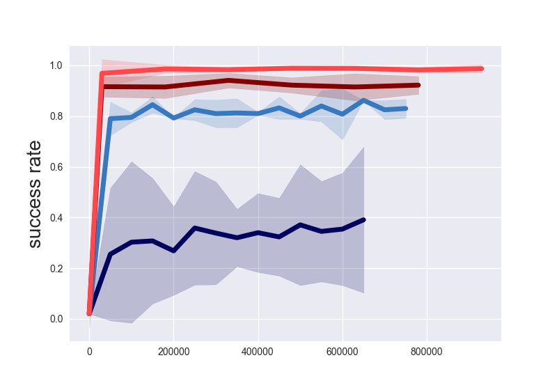
(a) Point mass

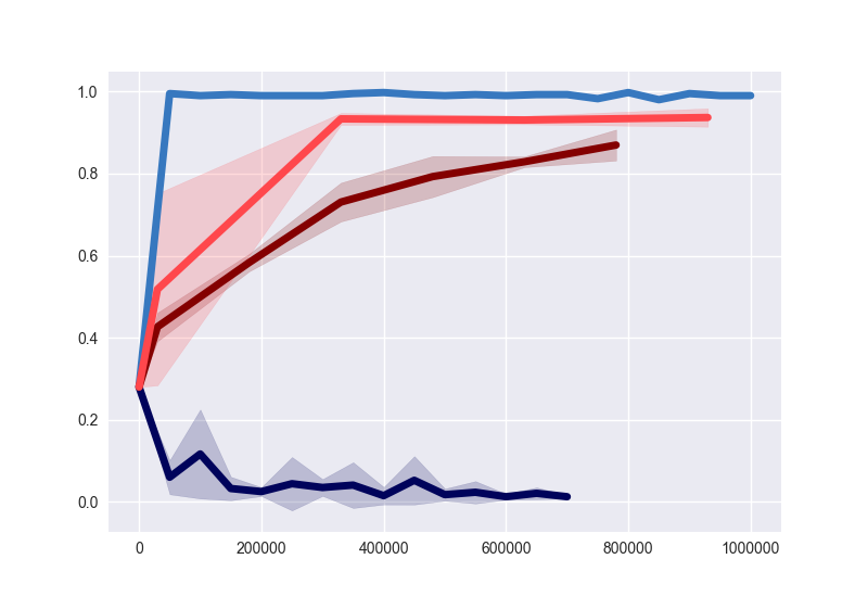
(b) Reacher goal

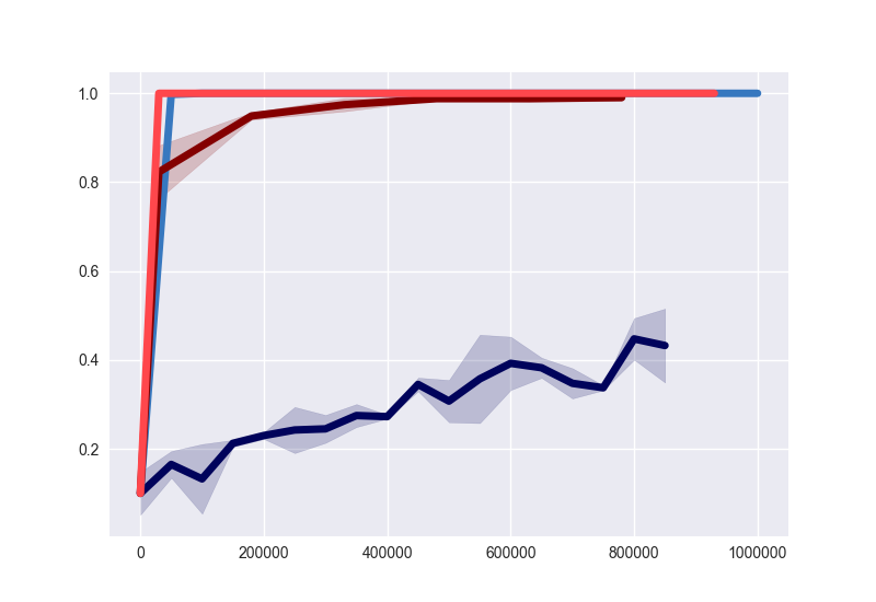
(c) Fetch robot

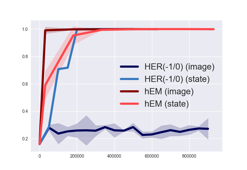
(d) Sawyer robot

Figure 1: Training curves of $\mathrm{h}$em and her on four goal-conditioned rl benchmark tasks. Inputs are either state-based or image-based. The y-axis shows the success rates and the x-axis shows the training time steps. All curves are calculated based on averages over $5$ random seeds. Here, her ($-1/0$) denotes her trained on rewards $r=-\mathbb{I}[\text{failure}]$, see Section 4 for details. $\mathrm{h}$em consistently performs better than or similar to her across all tasks. The performance gains are significant for high-dimensional image-based tasks.

Main idea.

We propose a probabilistic framework for goal-conditioned rl that formalizes the intuition of hindsight using ideas from statistical simulation. We equate the traditional rl objective to maximizing the evidence of our probabilistic model. This leads to a new algorithm, hindsight expectation maximization ($\mathrm{h}$em), which maximizes a tractable lower bound of the original objective [7]. A central insight is that the E-step naturally interprets hindsight replay as a special case of is.

Figure 1 compares $\mathrm{h}$em to her [2] on four goal-conditioned rl tasks with low-dimensional state and high-dimensional images as inputs. While $\mathrm{h}$em performs consistently well on both inputs, her struggles with image-based inputs. This is due to how her leverages hindsight replay within a temporal difference (td)-learning procedure; performance degrades sharply with the dimensionality of the inputs (as observed previously in [8, 9]; also see Section 4). In contrast, $\mathrm{h}$em leverages hindsight experiences through the lens of is, thus enabling better performance in high dimensions.

The rest of this section presents a quick background on goal-conditioned rl and probabilistic inference. Expert readers may jump ahead to Section 2.

Goal-conditioned rl.

Consider an agent that interacts with an environment in episodes. At the beginning of each episode, a goal $g\in\mathcal{G}$ is fixed. At a discrete time $t\geq 0$, an agent in state $s_{t}\in\mathcal{S}$ takes action $a_{t}\in\mathcal{A}$, receives a reward $r(s_{t},a_{t},g)\in\mathbb{R}$, and transitions to its next state $s_{t+1}\sim p(\cdot\mid s_{t},a_{t})\in\mathcal{S}$. This process is independent of goals. A policy $\pi(a\mid s,g):\mathcal{S}\times\mathcal{G}\mapsto\mathcal{P}(\mathcal{A})$ defines a map from state and goal to distributions over actions. Given a distribution over goals $g\sim p(\cdot)$, we consider the undiscounted episodic return $J(\pi)\coloneqq\mathbb{E}_{g\sim p(\cdot)}\big{[}\mathbb{E}_{\pi}[\sum_{t=0}^{T-1}r(s_{t},a_{t},g)]\big{]}$.

Probabilistic inference.

Consider data as observed random variables $x\in\mathcal{X}$. Each measurement $x$ is a discrete or continuous random variable. A likelihood $p_{\theta}(x\mid z)$ relates each measurement to latent variables $z\in\mathcal{Z}$ and unknown, but fixed, parameters $\theta$. The full probabilistic generative model specifies a prior over the latent variable $p(z)$. Bayesian inference requires computing the posterior $p(z\mid x)$ — an intractable task for all but a small class of simple models.

Variational inference approximates the posterior by matching a tractable density $q_{\phi}(z\mid x)$ to the posterior. The following calculation specifies this procedure:

$$\log p(x) =\log\mathbb{E}_{z\sim p(\cdot)}\left[p_{\theta}(x\mid z)\right]$$

$$=\log\mathbb{E}_{z\sim q_{\phi}(\cdot\mid x)}\left[p_{\theta}(x\mid z)\frac{p(z)}{q_{\phi}(z\mid x)}\right]$$

$$\geq\mathbb{E}_{z\sim q_{\phi}(\cdot\mid x)}\left[\log p_{\theta}(x\mid z)\frac{p(z)}{q_{\phi}(z\mid x)}\right]$$ (1)

$$=\mathbb{E}_{z\sim q_{\phi}(\cdot\mid x)}\left[\log p_{\theta}(x\mid z)\right]-\mathbb{KL}[q_{\phi}(\cdot\mid z)\;\|\;p(z)]$$

$$\eqqcolon L(p_{\theta},q).$$ (2)

(For a detailed derivation, please see [7].) Equation 2 defines the evidence lower bound (elbo) $L(p_{\theta},q)$. Matching the tractable density $q_{\phi}(z\mid x)$ to the posterior thus turns into maximizing the elbo via expectation maximization (em) [10] or stochastic gradient ascent [11, 12]. Figure 2(a) presents a graphical model of the above. For a fixed set of $\theta$ parameters, the optimal variational distribution $q$ is the true posterior $\arg\max_{q}L(p_{\theta},q)\equiv p(z\mid x)\coloneqq p(z)p_{\theta}(x\mid z)/p(x)$. From an is perspective, note how the variational distribution $q_{\phi}(z\mid x)$ serves as a proposal distribution in place of $p(z)$ in the derivation of Equation 1.

(a) Probabilistic inference

(b) Variational rl

(c) Goal-conditioned rl
(Generative model)

(d) Goal-conditioned rl
(Inference model)

Figure 2: Graphical models. Solid lines represent generative models and dashed lines represent inference models. Circles represent random variables and squares represent parameters. Shading indicates that the random variable is observed.

2 A Probabilistic Model for Goal-conditioned Reinforcement Learning

Probabilistic modeling and control enjoy strong connections, especially in linear systems [13, 14]. Two recent frameworks connect probabilistic inference to general rl: Variational rl [15, 16, 17, 18] and rl as inference [19, 20, 21]. We situate our probabilistic model by first presenting Variational rl below. (Appendix A presents a detailed comparison to rl as inference.)

Variational rl.

Begin by defining a trajectory random variable $\tau\equiv(s_{t},a_{t})_{t=1}^{T-1}$ to encapsulate a sequence of state and action pairs. The random variable is generated by a factorized distribution $a_{t}\sim\pi_{\theta}(\cdot\mid s_{t}),s_{t+1}\sim p(\cdot\mid s_{t},a_{t})$, which defines the joint distribution $p_{\theta}(\tau)\coloneqq\Pi_{t=0}^{T-1}\pi_{\theta}(a_{t}\mid s_{t})\;p(s_{t+1}\mid s_{t},a_{t})$. Conditional on $\tau$, define the distribution of a binary optimality variable as $p(O=1\mid\tau)\propto\exp(\sum_{t=0}^{T-1}r(s_{t},a_{t})/\alpha)$ for some $\alpha>0$, where we assume $r(s_{t},a_{t})\geq 0$ without loss of generality. Optimizing the standard rl objective corresponds to maximizing the evidence of $\log p(O=1)$, where all binary variables are treated as observed and equal to one. Positing a variational approximation to the posterior over trajectories gives the following lower bound,

$$\log p(O=1)\geq \;\mathbb{E}_{q(\tau)}\left[\log p(O=1\mid\tau)\right]-$$

$$\mathbb{KL}\left[q(\tau)\;\|\;p_{\theta}(\tau)\right]\eqqcolon L(\pi_{\theta},q).$$ (3)

Figure 2(b) shows a combined graphical model for both the generative and inference models of Variational rl. Equation 3 is typically maximized using em (e.g., [22, 17, 18]), by alternating updates between $\theta$ and $q(\tau)$. Note that Variational rl does not model goals.

2.1 Probabilistic goal-conditioned reinforcement learning

To extend the Variational rl framework to incorporate goals, introduce a goal variable $g$ and a prior distribution $g\sim p(\cdot)$. Conditional on a goal $g$, the trajectory variable $\tau\equiv(s_{t},a_{t})_{t=0}^{T-1}\sim p(\cdot\mid\theta,g)$ is sampled by executing the policy $\pi_{\theta}(a\mid s,g)$ in the Markov decision process (mdp). Similar to Variational rl, the joint distribution factorizes as $p(\tau\mid\theta,g)\coloneqq\Pi_{t=0}^{T-1}\pi_{\theta}(a_{t}\mid s_{t},g)p(s_{t+1}\mid s_{t},a_{t})$. Now, define a goal-conditioned binary optimality variable $O$, such that $p(O=1\mid\tau,g)\coloneqq R(\tau,g)\coloneqq\sum_{t=0}^{T-1}r(s_{t},a_{t},g)/\alpha$ where $\alpha>0$ normalizes this density. Figure 2(c) shows a graphical model of just this generative model. Treat the optimality variables as the observations and assume $O\equiv 1$. The following proposition shows the equivalence between inference in this model and traditional goal-conditioned rl.

Proposition 1.

(Proof in Appendix B.) Maximizing the evidence of the probabilistic model is equivalent to maximizing returns in the goal-conditioned rl problem, i.e.,

$$\arg\max_{\theta}\log p(O=1)=\arg\max_{\theta}J(\pi_{\theta}).$$ (4)

2.2 Challenges with direct optimization

Equation 4 implies that algorithms that maximize the evidence of such probabilistic models could be readily applied to goal-conditioned rl. Unlike typical probabilistic inference settings, the evidence here can technically be directly optimized. Indeed, $p(O=1)\equiv J(\pi_{\theta})$ could be maximized via traditional rl approaches e.g., policy gradients [23]. In particular, the reinforce gradient estimator [24] of Equation 4 is given by as $\eta_{\theta}=\sum_{t\geq 0}\sum_{t^{\prime}\geq t}r(s_{t^{\prime}},a_{t^{\prime}},g)\nabla_{\theta}\log\pi_{\theta}(a_{t}\mid s_{t},g)\approx\nabla_{\theta}J(\pi_{\theta})$, where $g\sim p(\cdot)$ and $(s_{t},a_{t})_{t=0}^{T-1}$ are sampled on-policy. The direct optimization of $\log p(O=1)$ consists of a gradient ascent sequence $\theta\leftarrow\theta+\eta_{\theta}$. However, this poses a practical challenge in goal-conditioned rl. To see why, consider the following example.

Illustrative example.

Consider a one-step mdp with $T=1$ where $\mathcal{S}=\{s_{0}\}$, $\mathcal{A}=\mathcal{G}$, $r(s,a,g)=\mathbb{I}[a=g]$. Assume that there are a finite number of actions and goals $|\mathcal{A}|=|\mathcal{G}|=k$.

The following theorem shows the difficulty in building a practical estimator for $\nabla_{\theta}J(\pi_{\theta})$.

Theorem 1.

(Proof in Section B.2.) Consider the example above. Let the policy $\pi_{\theta}(a\mid s,g)=\text{softmax}(L_{a,g})$ be parameterized by logits $L_{a,g}$ and let $\eta_{a,g}$ be the one-sample reinforce gradient estimator of $L_{a,g}$. Assume a uniform distribution over goals $p(g)=1/k$ for all $g\in\mathcal{G}$. Assume that the policy is randomly initialized (e.g. $L_{a,g}\equiv L,\forall a,g$ for some $L$). Let $\text{MSE}[x]$ be the mean squared error $\text{MSE}[x]\coloneqq\mathbb{E}[(x-\mathbb{E}[\eta_{a,g}])^{2}]$. It can be shown that the relative error of the estimate $\sqrt{\text{MSE}[\eta_{a,g}]}/\mathbb{E}[\eta_{a,g}]=k(1+o(1))$ grows approximately linearly with $k$ for all $\forall a\in\mathcal{A},g\in\mathcal{G}$.

The above theorem shows that in the simple setup above, the relative error of the reinforce gradient estimator grows linearly in $k$. This implies that to reduce the error with traditional Monte Carlo sampling would require $o(k^{2})$ samples, which quickly becomes intractable as $k$ increases. Though variance reduction methods such as control variates [25] could be of help, it does not change the sup-linear growth rate of samples (see comments in Section B.2). The fundamental bottleneck is that dense gradients, where $r(s,a,g)\nabla_{\theta}\log\pi_{\theta}(a\mid s,g)\neq 0$, are rare events with probability $\nicefrac{{1}}{{k}}$, which makes them difficult to estimate with on-policy measures [5]. This example hints at similar issues with more realistic cases and motivates an is approach to address the problem.

2.3 Tractable lower bound

Consider a variational inequality similar to Equation 2 with a variational distribution $q(\tau,g)$

$$\begin{split}\log p(O=1)&=\log\mathbb{E}_{q(\tau,g)}\left[p(O=1\mid\tau,g)\frac{p(g)p(\tau\mid\theta,g)}{q(\tau,g)}\right]\\ &\geq\mathbb{E}_{q(\tau,g)}\left[\log p(O=1\mid\tau,g)\frac{p(g)p(\tau\mid\theta,g)}{q(\tau,g)}\right]\\ &=\mathbb{E}_{q(\tau,g)}\left[\log p(O=1\mid\tau,g)\right]-\\ &\ \ \ \ \mathbb{KL}\left[q(\tau,g)\;\|\;p(g)p(\tau\mid\theta,g)\right]\\ &\eqqcolon L(\pi_{\theta},q).\end{split}$$ (5)

This variational distribution corresponds to the inference model in Figure 2(d). As with typical graphical models, instead of maximizing $\log p(O=1)$, consider maximizing its elbo $L(\pi_{\theta},q)$ with respect to both $\theta$ and variational distribution $q(\tau,g)$. Our key insight lies in the following observation: the bottleneck of the direct optimization of $\log p(O=1)$ lies in the sparsity of $p(O=1\mid\tau,g)=\sum_{t=0}^{T-1}r(s_{t},a_{t},g)$, where $(\tau,g)$ are sampled with the on-policy measure $g\sim p(\cdot),\tau\sim p(\cdot\mid\theta,g)$. The variational distribution $q(\tau,g)$ serves as a is proposal in place of $p(\tau\mid\theta,g)p(g)$. If $q(\tau,g)$ puts more probability mass on $(\tau,g)$ pairs with high returns (high $p(O=1\mid\tau,g)$), the rewards become dense and learning becomes feasible. In the next section, we show how hindsight replay [2] provides an intuitive and effective way to select such a $q(\tau,g)$.

3 Hindsight Expectation Maximization

The em-algorithm [10] for Equation 5 alternates between an E- and M-step: at iteration $t$, denote the policy parameter to be $\theta_{t}$ and the variational distribution to be $q_{t}$.

$$\text{E-step:}\ q_{t+1}=\arg\max_{q}L(\pi_{\theta_{t}},q),\$$

$$\text{M-step:}\ \theta_{t+1}=\arg\max_{\theta}L(\pi_{\theta},q_{t+1}).$$ (6)

This ensures a monotonic improvement in the elbo $L(\pi_{\theta_{t+1}},q_{t+1})\geq L(\pi_{\theta_{t}},q_{t})$. We discuss these two alternating steps in details below, starting with the M-step.

M-step: Optimization for $\pi_{\theta}$.

Fixing the variational distribution $q(\tau,g)$, to optimize $L(\pi_{\theta},q)$ with respect to $\theta$ is equivalent to

$$\max_{\theta}\mathbb{E}_{q(\tau,g)}\left[\log p(\tau\mid\theta,g)\right]$$

$$\equiv\max_{\theta}\mathbb{E}_{q(\tau,g)}\left[\sum_{t=0}^{T-1}\log\pi_{\theta}(a_{t}\mid s_{t},g)\right].$$ (7)

The right hand side of Equation 7 corresponds to a supervised learning problem where learning samples come from $q(\tau,g)$. Prior studies have adopted this idea and developed policy optimization algorithms in this direction [17, 18, 26, 27, 28]. In practice, the M-step is carried out partially where $\theta$ is updated with gradient steps instead of optimizing Equation 7 fully.

E-step: Optimization for $q(\tau,g)$.

The choice of $q(\tau,g)$ should satisfy two desirable properties: (P.1) it leads to monotonic improvements in $\log p(O=1)\equiv J(\pi_{\theta})$ or a lower bound thereof; (P.2) it provide dense learning signals for the M-step. The posterior distribution $p(\tau,g\mid O=1)$ achieves (P.1) and (P.2) in a near-optimal way, in that it is the maximizer of the E-step in Equation 6, which monotonically improves the elbo. The posterior also provides dense reward signals to the M-step because $p(\tau,g\mid O=1)\propto p(O=1\mid\tau,g)$. In practice, one chooses a variational distribution $q(\tau,g)$ as an alternative to the intractable posterior by maximizing Equation 5. Below, we show it is possible to achieve (P.1)(P.2) even though the E-step is not carried out fully. By plugging in $p(O=1\mid\tau,g)=\sum_{t=0}^{T-1}r(s_{t},a_{t},g)/\alpha$, we write the elbo as

$$L(\pi_{\theta},q)= \underbrace{\mathbb{E}_{q(\tau,g)}\Bigg{[}\frac{\sum_{t=0}^{T-1}r(s_{t},a_{t},g)}{\alpha}\Bigg{]}}_{\text{first\ term}}\,+\,$$

$$\underbrace{\vphantom{\Bigg{[}}-\mathbb{KL}[q(\tau,g)\;\|\;p(g)p(\tau\mid\theta,g)]}_{\text{second\ term}}.$$ (8)

We now examine alternative ways to select the variational distribution $q(\tau,g)$.

Prior work.

State-of-the-art model-free algorithms such as mpo [17, 18] applies a factorized variational distribution $q_{\text{ent}}(\tau,g)=p(g)\Pi_{t=0}^{T-1}q_{\text{ent}}(a_{t}\mid s_{t},g)$. The variational distribution is defined by local distributions $q_{\text{ent}}(a\mid s,g)\coloneqq\pi_{\theta}(a\mid s,g)\exp(\hat{Q}^{\pi_{\theta}}(s,a,g)/\eta)$ for some temperature $\eta>0$ and estimates of Q-functions $\hat{Q}^{\pi_{\theta}}(s,a,g)$. The design of $q_{\text{ent}}(\tau,g)$ could be interpreted as initializing $q_{\text{ent}}(a\mid s,g)$ with $\pi_{\theta}(a\mid s,g)$ which effectively maximizes the second term in Equation 8, then taking one improvement step of the first term [17]. This distribution satisfies (P.1) because the combined em-algorithm corresponds to entropy-regularized policy iteration, and retains monotonic improvements in $J(\pi_{\theta})$. However, it does not satisfy (P.2): when rewards are sparse $r(s,a,g)\approx 0$, estimates of Q-functions are sparse $Q^{\pi_{\theta}}(s,a,g)\approx 0$ and leads to uninformed variational distributions $q_{\text{ent}}(a\mid s)\propto\pi_{\theta}(a\mid s)\exp(Q^{\pi_{\theta}}(s,a,g)/\eta)\approx\pi_{\theta}(a\mid s,g)$ for the M-step. In fact, when $\eta$ is large and the update to $q(a\mid s)$ from $\pi_{\theta}(a\mid s,g)$ becomes infinitesimal, the E-step is equivalent to policy gradients [25, 23], which suffers from the sparsity of rewards as discussed in Section 2.

Hindsight variational distribution.

Maximizing the first term of the elbo is challenging when rewards are sparse. This motivates choosing a $q(\tau,g)$ which puts more weights on maximizing the first term. Now, we formally introduce the hindsight variational distribution $q_{h}(\tau,g)$, the sampling distribution employed equivalently in her [2]. Sampling from this distribution is implicitly defined by an algorithmic procedure:

Step 1.

Collect an on-policy trajectory or sample a trajectory from a replay buffer $\tau\sim\mathcal{D}$.

Step 2.

Find the $g$ such that the trajectory is rewarding, in that $R(\tau,g)$ is high or the trial is successful. Return the pair $(\tau,g)$.

Note that Step 2 can be conveniently carried out with access to the reward function $r(s,a,g)$ as in [2]. Contrary to $q_{\text{ent}}(\tau,g)$, this hindsight variational distribution maximizes the first term in Equation 8 by construction. This naturally satisfies (P.2) as $q_{h}(\tau,g)$ provides highly rewarding samples $(\tau,g)$ and hence dense signals to the M-step. The following theorem shows how $q_{h}(\tau,g)$ improves the sampling performance of our gradient estimates

Theorem 2.

(Proof in Section B.3.) Consider the illustrative example in Theorem 1. Let $\eta^{h}(a,g)=r(s,b,g^{\prime})\nabla_{L_{a,g}}\log\pi(b\mid s,g^{\prime})/k$ be the normalized one-sample reinforce gradient estimator where $(b,g^{\prime})$ are sampled from the hindsight variational distribution with an on-policy buffer. Then the relative error $\sqrt{\text{MSE}[\eta^{h}_{a,g}]}/\mathbb{E}[\eta_{a,g}]=\sqrt{k}(1+o(1))$ grows sub-linearly for all $\forall a\in\mathcal{A},g\in\mathcal{G}$.

Theorem 2 implies that to further reduce the relative error of the hindsight estimator $\eta^{h}(a,g)$ with traditional Monte Carlo sampling would require $m\approx(\sqrt{k})^{2}=k$ samples, which scales linearly with the problem size $k$. This is a sharp contrast to $m\approx k^{2}$ from using the on-policy reinforce gradient estimator. The above result shows the benefits of is, where under $q_{h}(\tau,g)$ rewarding trajectory-goal pairs are given high probabilities and this naturally alleviates the issue with sparse rewards. The following result shows that $q_{h}(\tau,g)$ also satisfies (P.1) under mild conditions.

Theorem 3.

(Proof in Section B.4.) Assume $p(g)$ to be uniform without loss of generality and a tabular representation of policy $\pi_{\theta}$. At iteration $t$, assume that the partial E-step returns $q_{t}(\tau,g)$ and the M-step objective in Equation 7 is optimized fully. Also assume the variational distribution to be the hindsight variational distribution $q_{t}(\tau,g)\coloneqq q_{h}(\tau,g)$. Let $\tilde{p}_{t}(g)\coloneqq\int_{\tau}q_{t}(\tau,g)d\tau$ be the marginal distribution of goals. The performance is lower bounded as $J(\pi_{\theta_{t+1}})\geq|\text{supp}(\tilde{p}_{t}(g))|/|\mathcal{G}|\eqqcolon\tilde{L}_{t}$. When the replay buffer size $\mathcal{D}$ increases over iterations, the lower bound improves $\tilde{L}_{t+1}\geq\tilde{L}_{t}$.

3.1 Algorithm

We now present $\mathrm{h}$em which combines the above E- and M-steps. The algorithm maintains a policy $\pi_{\theta}(a\mid s,g)$. At each iteration, $\mathrm{h}$em collects $N$ trajectory-goal pairs by first sampling a goal $g\sim p(\cdot)$ and then rolling out a trajectory $\tau$. Our initial experiments showed that exploration is critical when collecting trajectories. Under-exploration might drive $\mathrm{h}$em to sub-optimal solutions. For continuous action space, we modify the agent to execute $a^{\prime}=\mathcal{N}(0,\sigma_{a}^{2})+a$ where $a\sim\pi_{\theta}(a\mid s,g)$ and $\sigma_{a}=0.5$. This small amount of injected noise ensures that the algorithm has sufficient coverage of the state and goal space, which we find to be important for learning stability [29, 30]. After this collection phase, all trajectories are stored into a replay buffer $\mathcal{D}$ [3].

At training time, $\mathrm{h}$em carries out a partial E-step by sampling $(\tau,g)$ pairs from $q_{h}(\tau,g)$. In practice, given a trajectory $\tau$ uniformly sampled from the buffer, a target goal $g$ is sampled using the future strategy proposed in [2]. For the partial M-step, the policy is updated through stochastic gradient descents on Equation 7 with the Adam optimizer [31]. Importantly, $\mathrm{h}$em is an off-policy rl algorithm without value functions, which also makes it agnostic to reward functions. The pseudocode is summarized in Algorithm 1. Please refer to Appendix C for full descriptions of the algorithm.

1:  INPUT policy $\pi_{\theta}(a\mid s,g)$.

2:  while  $t=0,1,2...$  do

3:     Sample goal $g\sim p(\cdot)$ and trajectory $\tau\sim p(\cdot\mid\theta,g)$ by executing $\pi_{\theta}$ in the mdp. Save data $(\tau,g)$ to a replay buffer $\mathcal{D}$.

4:     E-step. Sample from $q_{h}(\tau,g)$: sample $\tau\equiv(s_{t},a_{t})_{t=0}^{T-1}\sim\mathcal{D}$ and find rewarding goals $g$.

5:     M-step. Update the policy by a few gradient ascents $\theta\leftarrow\theta+\nabla_{\theta}\log\sum_{t=0}^{T-1}\log\pi_{\theta}(a_{t}\mid s_{t},g)$.

6:  end while

Algorithm 1 Hindsight Expectation Maximization ($\mathrm{h}$em)

3.2 Connections to prior work

Hindsight experience replay.

The core of her lies in the hindsight goal replay [2]. Similar to $\mathrm{h}$em, her samples trajectory-goal pairs from the hindsight variational distribution $q_{h}(\tau,g)$ and minimize the Q-learning loss $\mathbb{E}_{(\tau,g)\sim q_{h}(\cdot)}[\sum_{t=0}^{T-1}(Q_{\theta}(s_{t},a_{t},g)-r(s_{t},a_{t},g)-\gamma\max_{a^{\prime}}Q_{\theta}(s_{i},a^{\prime},g))^{2}]$. The development of $\mathrm{h}$em in Section 3 formalizes this choice of the sampling distribution $q(\tau,g)\coloneqq q_{h}(\tau,g)$ as partially maximizing the elbo during an E-step. Compared to $\mathrm{h}$em, her learns a critic $Q_{\theta}(s,a,g)$. We will see in the experiments that such critic learning tends to be much more unstable when rewards are sparse and inputs are high-dimensional, as was also observed in [8, 9].

Hindsight policy gradient.

In its vanilla form, the hindsight policy gradient (hpg) considers on-policy stochastic gradient estimators of the rl objective [23] as $\mathbb{E}_{p(g)p(\tau\mid\theta,g)}[R(\tau,g)\nabla_{\theta}\log p(\tau\mid\theta,g)]$. Despite variance reduction methods such as control variates [25, 23], the unbiased estimators of hpg do not address the rare event issue central to sparse rewards mdp, where $R(\tau,g)\nabla_{\theta}\log p(\tau\mid\theta,g)$ taking non-zero values is a rare event under the on-policy measure $p(g)p(\tau\mid\theta,g)$. Contrast hpg to the unbiased is objective in Equation 5: $\mathbb{E}_{q(\tau,g)}[R(\tau,g)\nabla_{\theta}\log p(\tau\mid\theta,g)\cdot\frac{p(g)p(\tau\mid\theta,g)}{q(\tau,g)}]$, where the proposal $q(\tau,g)$ ideally prioritizes the rare events [5] to generate rich learning signals. $\mathrm{h}$em further avoids the explicit is ratios with the variational approach that leads to an elbo [7].

Related work on learning from hindsight.

[32, 33] propose imitation learning algorithms for goal-conditioned rl, which are similar to the M-step in Algorithm 1. While their algorithms are motivated from a purely behavior cloning perspective, we draw close connections between goal-conditioned rl and probabilistic inference based on graphical models. This new perspective of $\mathrm{h}$em decomposes the overall algorithms into two steps and clarifies their respective effects. Recently, hindsight policy improvement (hpi) [34] propose to model the joint distribution over trajectories and goals $p(g,\tau)$, which leads to similar em-based updates as $\mathrm{h}$em. Compared to hpi, $\mathrm{h}$em interprets the hindsight distribution (denoted as the relabeling distribution in [34]) as is proposals. In addition, $\mathrm{h}$em is specialized to sparse rewards while hpi is designed and evaluated for generic goal-conditioned rl problems with potentially dense reward signals.

With the E-step, $\mathrm{h}$em assigns more weights to rewarding $(\tau,g)$ pairs. Beyond goal-conditioned rl, This general idea of prioritizing samples with high returns has been combined with imitation learning [35, 36, 37], Q-learning [38] or model-based methods [39].

Supervised learning for rl.

The idea of applying supervised learning techniques in an iterative rl loop has been shown to stabilize the algorithms. In this space, successful examples include both model-based [40, 41, 42, 43] and model-free algorithms [44, 17, 27, 18]. As also evidenced by our own experiments in the next section, supervised learning is especially helpful for problems with high-dimensional image-based inputs (see also, e.g., [45, 46, 18, 42]).

Importance sampling in probabilistic inference.

Our work draws inspirations from the is views of recent probabilistic inference models. The use of is is inherent in the derivation of elbo [7]. Notably, for variational auto-encoders (vae) [11], [47] reinterpret the variational distribution $q_{\phi}(z\mid x)$ as an is proposal in place of the prior $p(z)$. This leads to a tighter elbo through the use of multiple importance-weighted samples, which is useful in some settings [48]. We expect such recent developments in probabilistic inference literature to be useful for future work in goal-conditioned rl.

4 Experiments

We evaluate the empirical performance of $\mathrm{h}$em on a wide range of goal-conditioned rl benchmark tasks. These tasks all have extremely sparse binary rewards which indicate success of the trial.

Baselines.

Since $\mathrm{h}$em builds on pure model-free concepts, we focus on the general purpose, model-free state-of-the-art algorithm her [2] as a comparison. In some cases we also compare with the closely-related hpg [23]. However, we find that even as hpg adopts more dense rewards, its performance evaluated as the success rate is inferior than her and $\mathrm{h}$em. We do not compare with other model-free baselines such as HPI [34], because they adopt a formulation of dense rewards and their code is not publicly available, making it difficult to make meaningful comparison. We also do not compare with algorithms which assume structured knowledge about the task such as [49, 50], though their combination with $\mathrm{h}$em is an interesting future direction. See Appendix C for more details.

Evaluations.

The evaluation criterion is the success rate at test time given a fixed budget on the total number of samples collected during training. For all evaluations in Figure 1, Figure 4 and Figure 5, we run $5$ runs of each algorithm and plot the $\text{mean}\pm\text{std}$ curves. Note that for many cases the standard deviations are small. We speculate this is because all experiments are run with $M\geq 20$ parallel workers for data collection and gradient computations, which reduces the performance variance across seeds.

Implementation details.

See Appendix C for full details on parameterizations of the policy in discrete and continuous action space, network architecture, data collection and hyper-parameters on training.

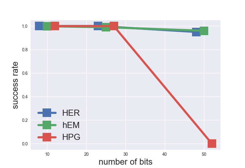
(a) Flip bit results

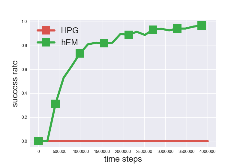
(b) Flip bit curves

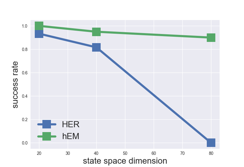
(c) Navigation results

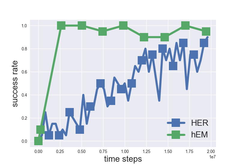
(d) Navigation curves

Figure 3: Summary of results for Flip bit and continuous navigation mdp. Plots (a) and (c) show the final performance after training is completed. Plots (b) and (d) show the training curves for Flip bit $K=50$ and navigation $K=40$ respectively. $\mathrm{h}$em consistently outperforms her and hpg across these tasks.

4.1 Simple examples

Flip bit.

Taken from [2], the mdp is parameterized by the number of bits $K$. The state space and goal space $\mathcal{S}=\mathcal{G}=\{0,1\}^{K}$ and the action space $\mathcal{A}=\{1,2,\ldots,K\}$. Given $s_{t}$, the action flips the bit at location $a_{t}$. The reward function is $r(s_{t},a_{t})=\mathbb{I}[s_{t+1}=g]$ , the state is flipped to match the target bit string. The environment is difficult for traditional rl methods as the search space is of exponential size $|\mathcal{S}|=2^{K}$. In Figure 3(a), we present results for her (taken from Figure 1 of [2]), $\mathrm{h}$em and hpg. Observe that $\mathrm{h}$em and her consistently perform well even when $K=50$ while the performance of hpg drops drastically as the underlying spaces become enormous. See Figure 3(b) for the training curves of $\mathrm{h}$em and hpg for $K=50$; note that hpg does not make any progress.

Continuous navigation.

As a continuous analogue of the Flip bit mdp, consider a $K$-dimensional navigation task with a point mass. The state space and goal space coincide with $\mathcal{X}=\mathcal{G}=[-1,1]^{K}$ while the actions $\mathcal{A}=[-0.2,0.2]^{K}$ specify changes in states. The reward function is $r(s_{t},a_{t})=\mathbb{I}[\;\|\;s_{t+1}-g\;\|\;<0.1]$ which indicates success when reaching the goal location. Results are shown in Figure 3(c) where we see that as $K$ increases, the search space quickly explodes and the performance of her degrades drastically. The performance of $\mathrm{h}$em is not greatly influenced by increases in $K$. See Figure 3(d) for the comparison of training curves between $\mathrm{h}$em and her for $K=40$. her already learns much more slowly compared to $\mathrm{h}$em and degrades further when $K=80$.

4.2 Goal-contitioned reaching tasks

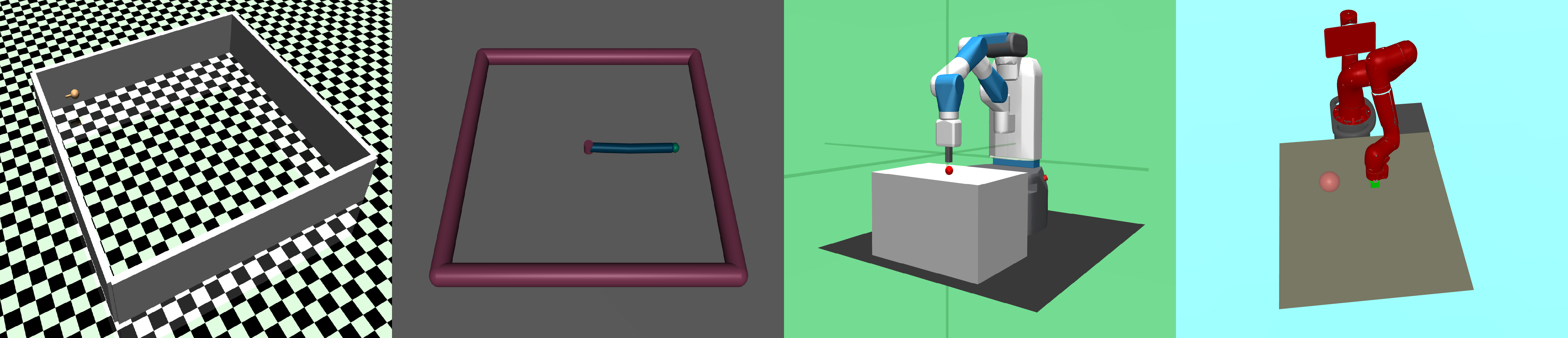
Figure 8: Illustration of tasks. From left to right: Point mass, Reacher, Fetch robot and Sawyer Robot. On the right is the image-based input for Fetch robot. For additional information on the tasks, see Appendix C.

To assess the performance of $\mathrm{h}$em in contexts with richer transition dynamics, we consider a wide range of goal-conditioned reaching tasks. We present details of their state space $\mathcal{X}$, goal space $\mathcal{G}$ and action space $\mathcal{A}$ in Appendix C. These include Point mass, Reacher goal, Fetch robot and Sawyer robot, as illustrated in Figure 8 in Appendix C.

Across all tasks, the reward takes the sparse form $r(s,a,g)=\mathbb{I}[\text{success}]$. As a comparison, we also include a her baseline where the rewards take the form $\tilde{r}(s,a,g)=-\mathbb{I}[\text{failure}]$. Such reward shaping does not change the optimality of policies as $\tilde{r}=r-1$ and is also the default rewards employed by e.g., the Fetch robot tasks. Surprisingly, this transformation has a big impact on the performance of her. We denote the her baseline under the reward $r=\mathbb{I}[\text{success}]$ as ‘her (0/1)’ and $\tilde{r}=-\mathbb{I}[\text{failure}]$ as ‘her (-1/0)’.

From the result in Figure 4, we see that $\mathrm{h}$em performs significantly better than her with binary rewards (her-sparse). The performance of $\mathrm{h}$em quickly converges to optimality while her struggles at learning good Q-functions. However, when compared with her ($-1/0$), $\mathrm{h}$em does not achieve noticeable gains. Such an observation confirms that her is sensitive to reward shaping due to the critic learning.

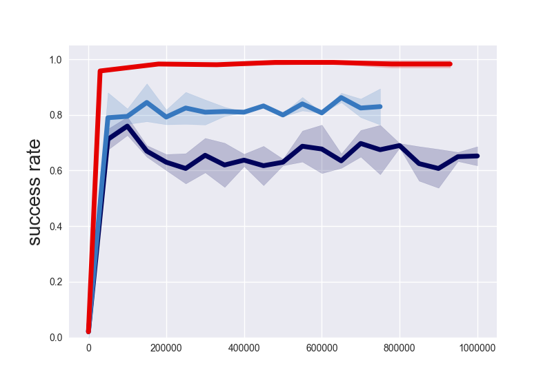
(a) Point mass

(b) Reacher goal

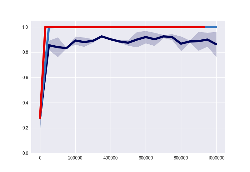
(c) Fetch robot

(d) Sawyer robot

Figure 4: Training curves of $\mathrm{h}$em and her on four goal-conditioned rl benchmark tasks with state-based inputs and sparse binary rewards. The y-axis shows the success rates and the x-axis shows the training time steps. All curves are calculated based on averages over $5$ random seeds. Standard deviations are small across seeds.

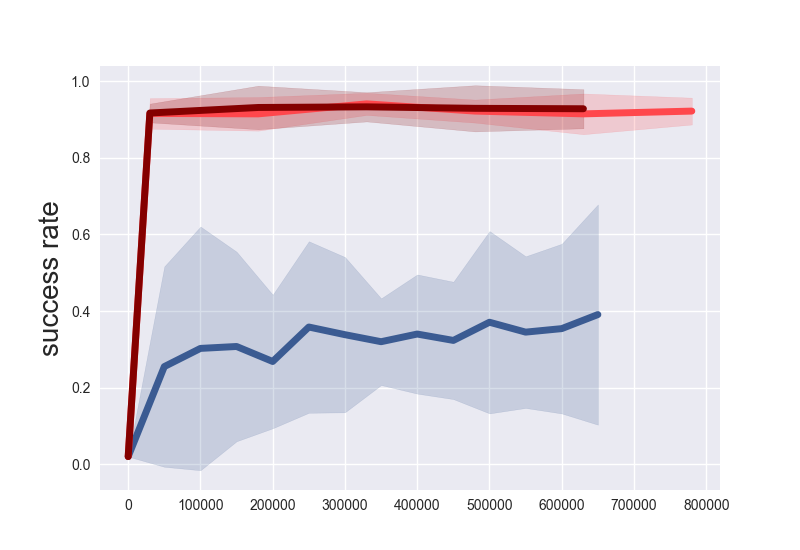
(a) Point mass (I)

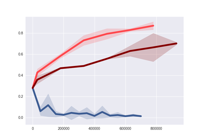
(b) Reacher goal (I)

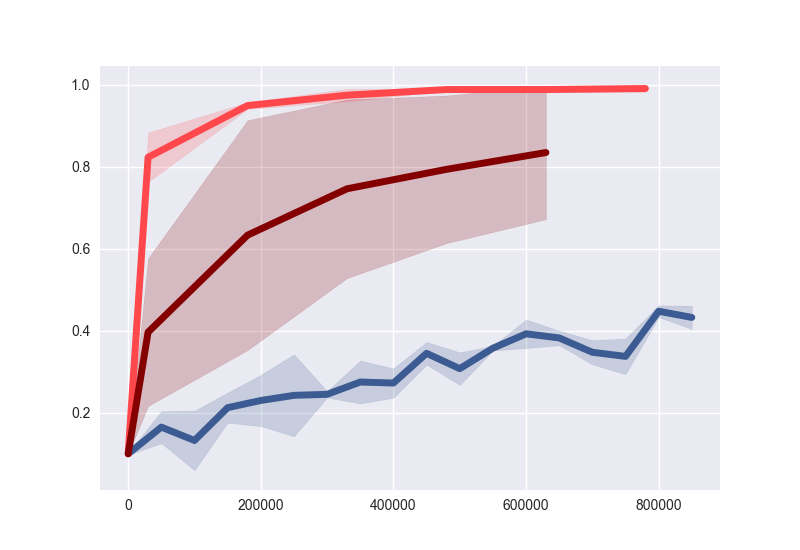
(c) Fetch robot (I)

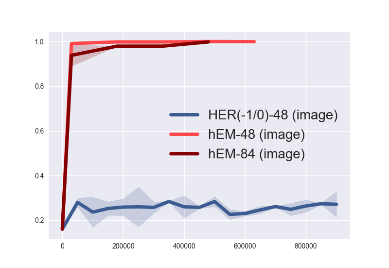
(d) Sawyer robot (I)

Figure 5: Training curves of $\mathrm{h}$em and her on four goal-conditioned rl tasks with image-based inputs. Standard deviations are small across seeds. All curves are calculated based on averages over $5$ random seeds. ‘$\mathrm{h}$em-48’ refers to image inputs with $w=48$. $\mathrm{h}$em achieves stable learning regardless of the input sizes, though larger sizes in general slow down the learning speed.

4.3 Image-based tasks

We further assess the performance of $\mathrm{h}$em when policy inputs are high-dimensional images (see Figure 9 for illustrations). Across all tasks, the state inputs are by default images $s\in\mathbb{R}^{w\times w\times 3}$ where $w\in\{48,84\}$ while the goal is still low-dimensional. See Appendix C for the network architectures.

We focus on the comparison between $\mathrm{h}$em and her ($-1/0$) in Figure 5, as the performance of her with binary rewards is inferior as seen Section 4.2. We see that for image-based tasks, her ($-1/0$) significantly underperforms $\mathrm{h}$em. While her ($-1/0$) makes slow progress for most cases, $\mathrm{h}$em achieves stable learning across all tasks. We speculate this is partly due to the common observations [8, 9] that td-learning directly from high-dimensional image inputs is challenging. For example, prior work [49] has applied a vae [11] to reduce the dimension of the image inputs for downstream td-learning. On the contrary, $\mathrm{h}$em only requires optimization in a supervised learning style, which is much more stable with end-to-end training on image inputs.

Further, image-based goals are much easier to specify in certain contexts [49]. We evaluate $\mathrm{h}$em on image-based goals for the Sawyer robot and achieve similar performance as the state-based goals. See results in Figure 10 in Appendix C.

4.4 Goal-conditioned Fetch tasks

Finally, we evaluate the performance of her and $\mathrm{h}$em over the full suite of Fetch robot tasks introduced in [2]. These Fetch tasks have the same transition dynamics as the previous Fetch Reach task, but differ significantly in the goal space. As a result, some of the tasks are more challenging than Fetch Reach due to difficulties in efficiently exploring the goal space. To tackle this issue, we implement a hybrid algorithm between $\mathrm{h}$em and her by combining their policy updates. In particular, we propose to update policy $\pi_{\theta}$ by considering the following hybrid objective,

$$L(\theta)= \underbrace{\mathbb{E}_{(s,g)\sim\mathcal{D}}\left[Q_{\phi}\left(s,\pi_{\theta}(s),g\right)\right]}_{\text{HER}}+$$

$$\eta\cdot\underbrace{\mathbb{E}_{q(\tau,g)}\left[\sum_{t=0}^{T-1}\log\pi_{\theta}(a_{t}\mid s_{t},g)\right]}_{\text{hEM}}.$$

The policy is updated as $\theta\leftarrow\theta+\nabla_{\theta}L(\theta)$. The Q-function $Q_{\phi}(s,a,g)$ is trained with td-learning to approximate the true Q-function $Q_{\phi}\approx Q^{\pi_{\theta}}$. We see that the two terms echo the loss functions employed by her and $\mathrm{h}$em respectively. The constant coefficient $\eta\geq 0$ trades-off the two loss functions. We find $\eta=0.1$ to perform uniformly well on all selected tasks.

Besides loss functions, the algorithm collects data using the same procedure as her. This allows $\mathrm{h}$em to leverage potentially more efficient exploration schemes of her (e.g., correlated exploration noises). We find that the hybrid algorithm achieves marginal improvements in the learning speed compared to her, see Figure 6 for the comparison and full results in Appendix C.

Remark.

Exploration is an under-explored yet critical area in goal-conditioned rl, especially for tasks with hierarchical goal space and long horizons. Consistent with the observations in recent work [2], we find that under-exploration could lead to sub-optimal policies. We believe when combined with recent advances in exploration for goal-conditioned rl [51, 52], the performance of $\mathrm{h}$em could be further stabilized.

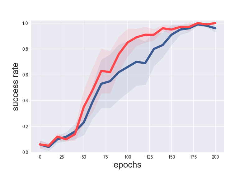
(a) Push

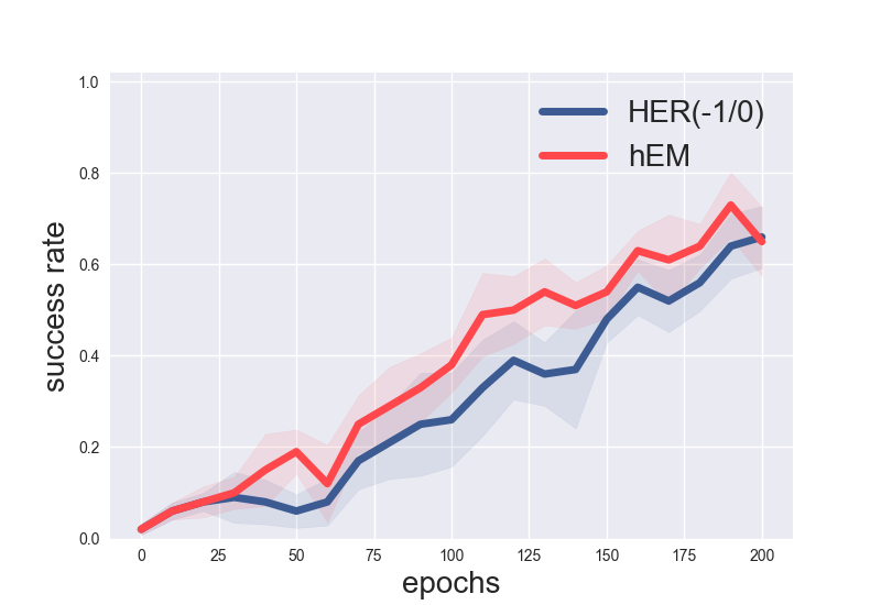
(b) Pick and Place

Figure 6: Fetch tasks. Training curves of $\mathrm{h}$em and her on two standard Fetch tasks. $\mathrm{h}$em provides marginal speed up compared to her. All curves are calculated based on $5$ random seeds. The x-axis shows the training epochs.

4.5 Ablation study

Recall that the $\mathrm{h}$em alternates between collecting $N$ trajectories and updating parameters via the em algorithm. We find the hyper-parameter $N$ impacts the algorithm significantly. Intuitively, the amount of collected data at each iteration implicitly determines the effective coverage of the goal space through exploration. When $N$ is small, the training might easily converge to local optima. See Figure 10 in Appendix C for full results. Both tasks in the ablation are challenging, due to an enormous state space or the high dimensionality of the inputs. In general, we find that larger $N$ leads to better performance (note that here the performance is always measured with a fixed budget on the total time steps). Similar observations have been made for her [2], where increasing the number of parallel workers generally improves training performance.

5 Conclusion

We present a probabilistic framework for goal-conditioned rl. This framework motivates the development of $\mathrm{h}$em, a simple and effective off-policy rl algorithm. Our formulation draws formal connections between hindsight goal replay [2] and is for rare event simulation. $\mathrm{h}$em combines the stability of supervised learning updates via the M-step and the hindsight replay technique via the E-step. We show improvements over a variety of benchmark rl tasks, especially in high-dimensional input settings with sparse binary rewards.

Acknowledgements.

The authors would like to acknowledge the computation support of Google Cloud Platform.

Appendix A Details on Graphical Models for Reinforcement Learning

In this section, we review details of the rl as inference framework [53, 21] and highlight its critical differences from Variational rl.

The graphical model for rl as inference is shown in Figure 7(c). The framework also assumes a trajectory variable $\tau\equiv(s_{t},a_{t})_{t=0}^{T-1}$ which encompasses the state and action sequences. Conditional on the trajectory variable $\tau$, the optimality variable is defined as $p(O=1\mid\tau)\propto\exp(\sum_{t=0}^{T-1}r(s_{t},a_{t})/\alpha)$ for $\alpha>0$. Under this framework, the trajectory variable has a prior $a_{t}\sim p(\cdot)$ where $p(\cdot)$ is usually set to be a uniform distribution over the action space $\mathcal{A}$.

The policy parameter $\theta$ comes into play with the inference model. The framework asks the question: what is the posterior distribution $p(\tau\mid O=1)$. To approximate this intractable posterior distribution, consider the variational distribution $q(\tau)\coloneqq\Pi_{t=0}^{T-1}\pi_{\theta}(a_{t}\mid s_{t})p(s_{t+1}\mid s_{t},a_{t})$. Searching for the best approximate posterior by minimizing the KL-divergence $\mathbb{KL}[q(\tau)\;\|\;p(\tau\mid O=1)]$, it can be shown that this is equivalent to maximum-entropy rl [54, 55, 56]. It is important to note that rl as inference does not contain trainable parameters for the generative model.

Contrasting this to Variational rl and the graphical model for goal-conditioned rl in Figure 2: the policy dependent parameter $\theta$ is part of a generative model. The variational distribution $q(\tau,g)$, defined separately from $\theta$, is the inference model. In such cases, the variational distribution $q(\tau,g)$ is an auxiliary distribution which aids in the optimization of $\theta$ by performing partial E-steps.

(a) Probabilistic inference

(b) Variational rl

(c) rl as inference

Figure 7: Plot (c) shows the graphical model for rl as inference [53, 21]. Solid lines represent generative models and dashed lines represent inference models. Circles represent random variables and squares represent parameters. Filled circles represent observed random variables. This graphical model does not have trainable parameters for the generative model. The policy dependent parameter $\theta$ is in the inference model.

Appendix B Details on proof

B.1 Proof of Proposition Proposition 1

The proof follows from the observation that $p(O=1)=\mathbb{E}_{g\sim p(\cdot),\pi}[p(O=1\mid\tau,g)]=J(\pi_{\theta})$, and taking the log does not change the optimal solution.

B.2 Proof of Theorem 1

Recall that we have a one-step mdp setup where $\mathcal{A}=\mathcal{G}$ and $|\mathcal{A}|=k$. The policy $\pi(a\mid s,g)=\text{softmax}(L_{a,g})$ is parameterized by logits $L_{a,g}$. When the policy is initialized randomly, we have $L_{a,g}\equiv L$ for some $L$ and $\pi(a\mid s,g)=1/k$ for all $a,g$. Assume also $p(g)=1/k,\forall g$.

The one-sample reinforce gradient estimator for the component $L_{a,g}$ is $\eta_{a,g}=r(s,b,g^{\prime})\log_{L_{a,g}}\pi(b\mid s,g^{\prime})$ with $g^{\prime}\sim p(\cdot)$ and $b\sim\pi(\cdot\mid s,g^{\prime})$. Further, we can show

$$\mathbb{E}[\eta_{a,g}]=\frac{1}{k^{2}}\delta_{a,g}-\frac{1}{k^{3}},\ \mathbb{V}[\eta_{a,g}]=(\frac{1}{k^{2}}+\frac{2}{k^{5}}-\frac{2}{k^{3}}-\frac{1}{k^{4}})\delta_{a,g}+\frac{1}{k^{4}}-\frac{1}{k^{6}},$$

where $\delta_{a,b}$ are dirac-delta functions, which mean $\delta_{a,b}=1$ if $a=b$ and $\delta_{a,b}=0$ otherwise. Taking the ratio, we have the squared relative error (note that the estimator is unbiased and MSE consists purely of the variance)

$$\frac{\text{MSE}[\eta_{a,g}]}{\mathbb{E}[\eta_{a,g}]^{2}}=\frac{(k^{4}+o(k^{4}))\delta_{a,g}+(k^{2}+o(k^{2}))}{(k^{2}+o(k^{2}))\delta_{a,g}+1}$$

The expression takes different forms based on the delta-function $\delta_{a,g}$. However, in either case (either $\delta_{a,g}=1$ or $\delta_{a,g}=0$), it is clear that $\frac{\text{MSE}[\eta_{a,g}]}{\mathbb{E}[\eta_{a,g}]^{2}}=k^{2}(1+o(1))$, which directly reduces to the result of the theorem.

Comment on the control variates.

We also briefly study the effect of control variates. Let $X,Y$ be two random variables and assume $\mathbb{E}[Y]=0$. Then compare the variance of $\mathbb{V}[X]$ and $\mathbb{V}[X+\alpha Y]$ where $\alpha$ is chosen optimally to minimize the variance of the second estimator. It can be shown that with the best $\alpha^{\ast}$, the ratio of variance reduction is $(\mathbb{V}[X]-\mathbb{V}[X+\alpha^{\ast}Y])/\mathbb{V}[X]=\rho^{2}\coloneqq\text{Cov}^{2}[X,Y]/\mathbb{V}[X]\mathbb{V}[Y]$. Consider the state-based control variate for the reinforce gradient estimator, in this case $-\alpha\cdot\nabla_{L_{a,g}}\pi(b\mid s,g^{\prime})$ where $\alpha$ is chosen to minimize the variance of the following aggregate estimator

$$\eta_{a,g}(\alpha)=r(s,b,g^{\prime})\log_{L_{a,g}}\pi(b\mid s,g^{\prime})-\alpha\log_{L_{a,g}}\pi(b\mid s,g^{\prime}).$$

Note that in practice, $\alpha$ is chosen to be state-dependent for reinforce gradient estimator of general MDPs and is set to be the value function $\alpha\coloneqq V^{\pi}(s)$. Such a choice is not optimal [57] but is conveniently adopted in practice. Here, we consider an optimal $\alpha^{\ast}$ for the one-step mdp. The central quantity is the squared correlation $\rho^{2}$ between $r(s,b,g^{\prime})\log_{L_{a,g}}\pi(b\mid s,g^{\prime})$ and $\log_{L_{a,g}}\pi(b\mid s,g^{\prime})$. With similar computations as above, it can be shown that $\rho^{2}\approx 1$ for $b\neq g^{\prime}$ and $\rho^{2}\approx\frac{1}{k^{2}}$ otherwise. This implies that for $k$ out of $k^{2}$ logits parameters, the variance reduction is significant; yet for the rest of the $k^{2}-k$ parameters, the variance reduction is negligible. Overall, the analysis reflects that conventional control variantes do not address the issue of sup-linear growth of relative errors as a result of sparse gradients.

B.3 Proof of Theorem 2

The key to the proof is the same as the proof of theorem 1: we analytically compute $\mathbb{E}[\eta_{a,g}]$ and $\mathbb{V}[\eta_{a,g}]$. We can show

$$\mathbb{E}[\eta_{a,g}]=\frac{1}{k^{2}}\delta_{a,g}+o(\frac{1}{k^{2}}),\ \mathbb{V}[\eta_{a,g}]=\frac{1}{k^{3}}\delta_{a,g}+o(\frac{1}{k^{3}}),$$

More specifically, it is possible to show that the normalized one-step reinforce gradient estimator $\eta^{h}_{a,g}=r(s,b,g^{\prime})\nabla_{L_{a,g}}\log\pi(b\mid s,g^{\prime})/k$ with $(b,g^{\prime})\sim q_{h}(\tau,g)$ has the following property

$$\frac{\text{MSE}[\eta_{a,g}]}{\mathbb{E}[\eta_{a,g}]^{2}}=\frac{(k^{3}+o(k^{3}))\delta_{a,g}+(k+o(k))}{(k^{2}+o(k))\delta_{a,g}+1}.$$

The above equality implies the result of the theorem. Indeed, the above implies regardless of whether $\delta_{a,g}=0$ or $\delta_{a,g}=1$: $\frac{\text{MSE}[\eta_{a,g}]}{\mathbb{E}[\eta_{a,g}]^{2}}=k(1+o(1))$.

Remark.

Contrast this with the result from Theorem 1, where the result is $k^{2}(1+o(1))$. The main difference stems from the variance: in Theorem 1 the variance is of order $\frac{1}{k^{2}}$ while here the variance is of order $\frac{1}{k^{3}}$. The variance reduction leads to significant improvements of the sample efficiency of the estimation.

B.4 Proof of Theorem 3

Without loss of generality we assume $p(g)$ is a uniform measure, i.e. $p(g)=1/|\mathcal{G}|$. If not, we could always find a transformation $g=f(g^{\prime})$ such that $g^{\prime}$ takes a uniform measure [6] and treat $g^{\prime}$ as the goal to condition on.

Let $|\mathcal{G}|<\infty$ and recall $\text{supp}(\tilde{p}(g))$ to be the support of $\tilde{p}(g)$. The uniform distribution assumption deduces that $|\text{supp}(\tilde{p}(g))|=\int_{g\in\text{supp}(\tilde{p}(g))}dg$. At iteration $t$, under tabular representation, the M-step update implies that $\pi_{\theta}$ learns the optimal policy for all $g$ that could be sampled from $q(\tau,g)$, whhich effectively corresponds to the support of $\tilde{p}(g)$. Formally, this implies $\mathbb{E}_{p(\tau\mid\theta_{t+1},g)}[R(\tau,g)]=1$ for $\forall g\in\text{supp}(\tilde{p}_{t}(g))$. This further implies

$$J(\pi_{\theta_{t+1}})\coloneqq\int\mathbb{E}_{p(\tau\mid\theta_{t+1},g)}[R(\tau,g)]p(g)dg\geq\int_{g\in\text{supp}(\tilde{p}_{t}(g))}1\cdot p(g)dg=|\text{supp}(\tilde{p}_{t}(g))|/|\mathcal{G}|.$$

Appendix C Additional Experiment Results

C.1 Details on Benchmark tasks

All reaching tasks are built with physics simulation engine MuJoCo [58]. We build customized point mass environment; the Reacher and Fetch environment is partly based on OpenAI gym environment [59]; the Sawyer environment is based on the multiworld open source code https://github.com/vitchyr/multiworld.

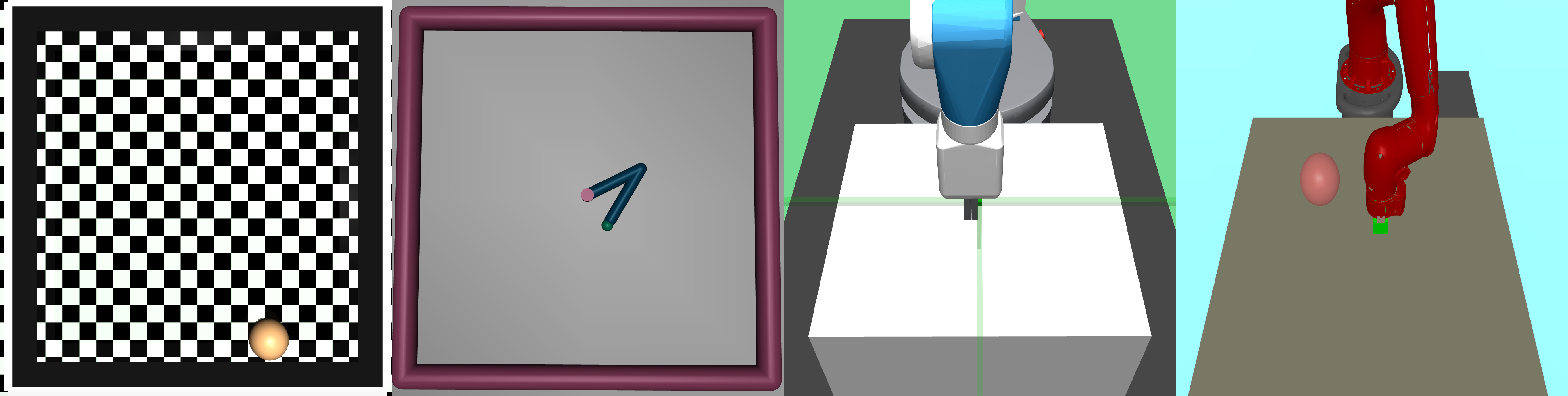
Figure 9: Illustration of image-based inputs for different reaching tasks in the main paper. Images are down-sampled to be of size $w\times w\times 3$ as inputs, where $w\in\{48,84\}$.

All simulation tasks below have a maximum episode length of $T=50$. The episode terminates early if the goal is achieved at a certain step. The sparse binary reward function is $r(s,a,g)=\mathbb{I}[\text{success}]$, which indicates the success of the transitioned state $s^{\prime}=f(s,a)$. Below we describe in details the setup of each task, in particular the success criterion.

• Point mass [32]. The objective is to navigate a point mass through a 2-D room with obstacles to the target location. $|\mathcal{S}|=4,|\mathcal{G}|=2$ and $|\mathcal{A}|=2$. The goals $g\in\mathbb{R}^{2}$ are specified as a 2-D point on the plane. Included in the state $s$ are the 2-D coordinates of the point mass, denoted as $s_{xy}\in\mathbb{R}^{2}$. The success is defined as $d(z(s_{xy}),z(g))\leq d_{0}$ where $d(\cdot,\cdot)$ is the Euclidean distance, $z(g)$ is a element-wise normalization function $z(x)\coloneqq(x-x_{\text{min}})/(x_{\text{max}}-x_{\text{min}})$ where $x_{\text{max}},x_{\text{min}}$ are the boundaries of the wall. The normalized threshold is $d_{0}=0.02\cdot\sqrt{2}$.

• Reacher [59]. The objective is to move via joint motors the finger tip of a 2-D Reacher robot to reach a target goal location. $|\mathcal{S}|=11,|\mathcal{G}|=2$ and $|\mathcal{A}|=2$. As with the above point mass environment, the goals $g\in\mathbb{R}^{2}$ are locations of a point at the 2-D plane. Included in the state $s$ are 2-D coordinates of the finger tip location of the Reacher robot $s_{xy}$. The success criterion is defined identically as the point mass environment.

• Fetch robot [59, 2]. The objective is to move via position controls the end effector of a fetch robot, to reach a target location in the 3-D space. $|\mathcal{S}|=10,|\mathcal{G}|=3$ and $|\mathcal{A}|=3$. This task belongs to the standard environment in OpenAI gym [59] and we leave the details to the code base and [2].

• Sawyer robot [49, 50]. The objective is to move via motor controls of the end effector of a sawyer robot, to reach a target location in the 3-D space. $|\mathcal{S}|=|\mathcal{G}|=|\mathcal{A}|=3$. This task belongs to the multiworld code base.

Details on image inputs.

For the customized point mass and Reacher environments, the image inputs are taken by cameras which look vertically down at the systems For the Fetch robot and Sawyer robot environment, the images are taken by cameras mounted to the robotic systems. See Figure 9 for an illustration of the image inputs.

C.2 Details on Algorithms and Hyper-parameters

Hindsight Expectation Maximization.

For $\mathrm{h}$em on domains with discrete actions, the policy is a categorical distribution $\pi_{\theta}(a\mid s,g)=\text{Cat}(\phi_{\theta}(s,g))$ with parameterized logits $\phi_{\theta}(s,g)$; on domains with continuous actions, the policy network is a state-goal conditional Gaussian distribution $\pi_{\theta}(a\mid s,g)=\mathcal{N}(\mu_{\theta}(s,g),\sigma^{2})$ with a parameterized mean $\mu_{\theta}(s,g)$ and a global standard deviation $\sigma^{2}$. The mean is takes the concatenated vector $[x,g]$ as inputs, has $5$ hidden layers each with $5$ hidden units interleaved with $\text{relu}(x)$ non-linear activation functions, and outputs a vector $\mu_{\theta}(s,g)\in\mathbb{R}^{|\mathcal{A}|}$.

$\mathrm{h}$em alternates between data collection using the policy and policy optimization with the em-algorithms. During data collection, the output action is perturbed by a Gaussian noise $a^{\prime}=\mathcal{N}(0,\sigma_{a}^{2})+a,a\sim\pi_{\theta}(\cdot\mid s,g)$ where the scale is $\sigma_{a}=0.5$. Note that injecting noise to actions is a common practice in off-policy rl algorithms to ensure sufficient exploration [3, 4]; for tasks with a discrete action space, the agent samples actions $a\sim\pi_{\theta}(\cdot\mid s,g)$ with probability $1-\epsilon$ and uniformly random with probability $\epsilon\in[0.2,0.5]$. The baseline $\mathrm{h}$em collects data with $N=30$ parallel MPI actors, each with $k=20$ trajectories. When sampling the hindsight goal given trajectories, we adopt the future strategy specified in her [2]: in particular, at state $s$, future achieved goals are uniformly sampled at trainig time as $q_{h}(\tau,g)$. All parameters are optimized with Adam optimizer [31] with learning rate $\alpha=10^{-3}$ and batch size $B=64$. By default, we run $M=30$ parallel MPI workers for data collection and training, at each iteration $\mathrm{h}$em collects $N=20$ trajectories from the environment. For image-based reacher and Fetch robot, $\mathrm{h}$em collects $N=80$ trajectories.

Hindsight Experience Replay.

By design in [2], her is combined with off-policy learning algorithms such as DQN or DDPG [3, 4]. We describe the details of DDPG. The algorithm maintains a Q-function $Q_{\theta}(s,a,g)$ parameterized similarly as a universal value function [60]: the network takes as inputs the concatenated vector $[x,a,g]$, has $5$ hidden layers with $h=256$ hidden units per layer interleaved with $\text{relu}(x)$ non-linear activation functions, and outputs a single scalar. The policy network $\pi_{\theta}(s,g)$ takes the concatenated vector $[x,g]$ as inputs, has the same intermediate architecture as the Q-function network and outputs the action vector $\pi_{\theta}(s,g)\in\mathbb{R}^{|\mathcal{A}|}$. We take the implementation from OpenAI baseline [61], all missing hyper-parameters are the default hyper-parameters in the code base. Across all tasks, her is run with $M=20$ parallel MPI workers as specified in [61].

Image-based architecture.

When state or goal are image-based, the Q-function network/policy network applies a convolutional network to extract features. For example, let $s,g\in\mathbb{R}^{w\times w\times 3}$ where $w\in\{48,84\}$ be raw images, and let $f_{\theta}(s),f_{\theta}(g)$ be the features output by the convolutional network. These features are concatenated before passing through the fully-connected networks described above. The convolutional network has the following architecture: $[32,8,4]\rightarrow\text{relu}\rightarrow[64,4,2]\rightarrow\text{relu}\rightarrow[64,3,2]\rightarrow\text{relu}$, where $[n_{f},r_{f},s_{f}]$ refers to: $n_{f}$ number of feature maps, $r_{f}$ feature patch dimension and $s_{f}$ the stride.

C.3 Ablation study

Ablation study on the effect of $N$.

$\mathrm{h}$em collects $N$ trajectories at each training iteration. We vary $N\in\{5,10,20,40,80\}$ on two challenging domains: Flip bit $K=50$ and Fetch robot (image-based) and evaluate the corresponding performance. See Figure 10. We see that in general, large $N$ tends to lead to better performance. For example, when $N=5$, $\mathrm{h}$em learns slowly on Flip bit; when $N=80$, $\mathrm{h}$em generally achieves faster convergence and better asymptotic performance across both tasks. We speculate that this is partly because with large $N$ the algorithm can have a larger coverage over goals (larger support over goals in the language of Theorem 3). With small $N$, the policy might converge prematurely and hence learn slowly. Similar observations have been made for her, where they find that the algorithm performs better with a large number of MPI workers (effectively large $N$).

Ablation on image-based goals.

To further assess the robustness of $\mathrm{h}$em against image-based inputs, we consider Sawyer robot where both states and goals are image-based. This differs from experiments shown in Figure 5 where only states are image-based. In Figure 10(c), we see that the performance of $\mathrm{h}$em does not degrade even when goals are image-based and is roughly agnostic to the size of the image. Contrast this with her, which does not make significant progress even when only states are image-based.

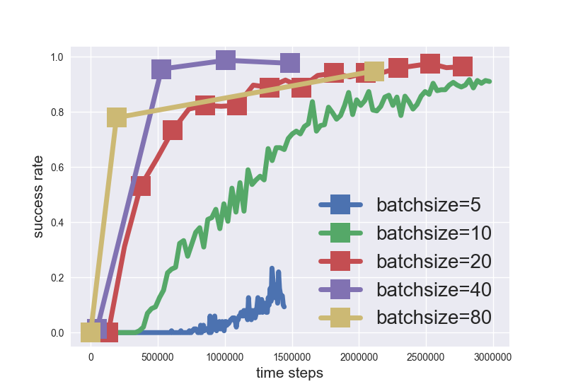
(a) Flip bit

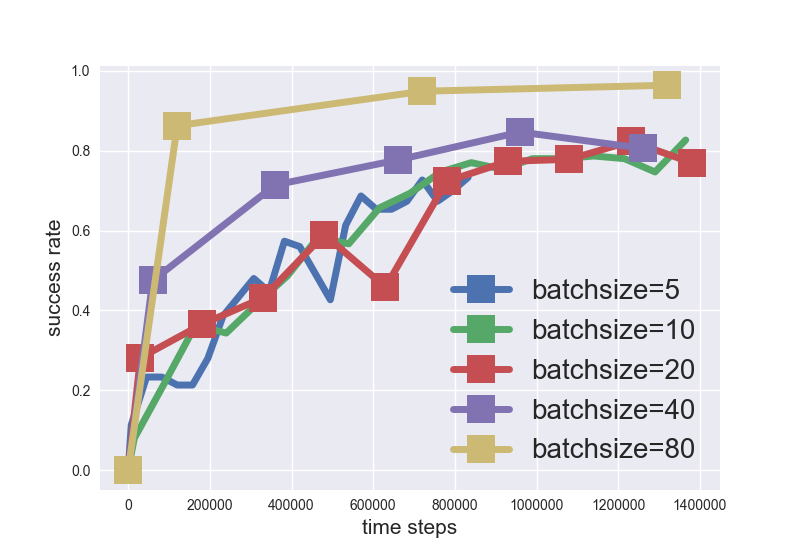
(b) Fetch robot

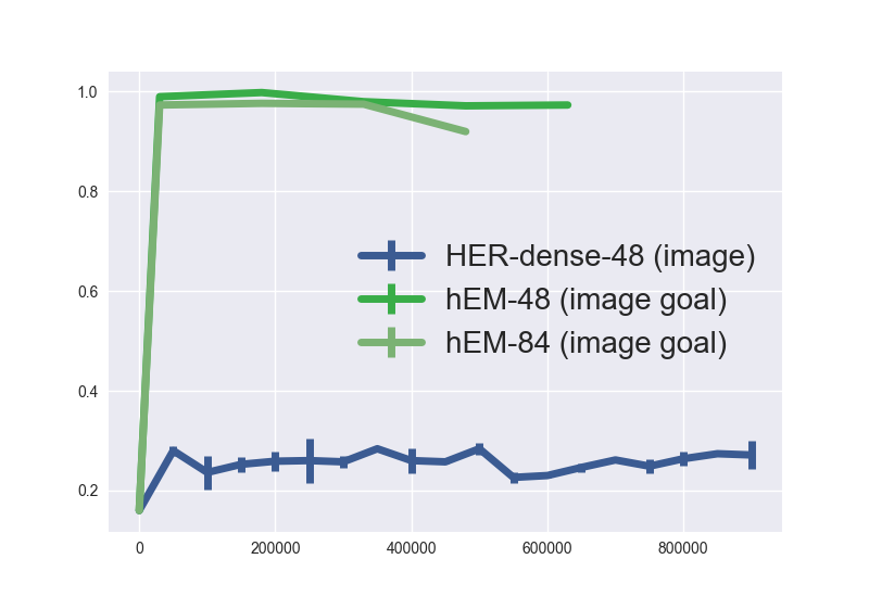
(c) Sawyer robot

Figure 10: Ablation study. Plot (a) and (b): The effect of the data collection size $N$. Plot (c): The effect of image-based inputs for both states and goals. ‘$\mathrm{h}$em-48’ refers to image-based inputs with size $48\times 48\times 3$. Note also ‘her-dense’ is equivalent to ‘her’($-1/0$) - though the reward function does not provide additional information compared to $(0/1)$, in practice this transformation makes the learning much more stable.

C.4 Comparison between $\mathrm{h}$em and hpg

We do not list hpg as a major baseline for comparison in the main paper, primarily due to a few reasons: by design, the hpg agent tackles discrete action space (see the author code base https://github.com/paulorauber/hpg), while many goal-conditioned baselines of interest [2, 49, 50] are continuous action space. Also, in [23] the author did not report comparison to traditional baselines such as her and only report cumulative rewards instead of success rate as evaluation criterion. Here, we compare $\mathrm{h}$em with hpg on a few discrete benchmarks provided in [23] to assess their performance.

Details on hpg.

The hpg is based on the author code base. [23] proposes several hpg variants with different policy gradient variance reduction techniques [25] and we take the hpg variant with the highest performance as reported in the paper. Throughout the experiment we set the learning rate to be $10^{-3}$ and other hyper-parameters take default values.

Benchmarks.

We compare $\mathrm{h}$em and hpg on Flip bit $K=25,50$ and the four room environment. The details of the Flip bit environment could be found in the main paper. The four room environment is used as a benchmark task in [23], where the agent navigates a grid world with four rooms to reach a target location within episodic time limit. The agent has access to four actions, which moves the agent in four directions. The trial is successful only if the agent reaches the goal in time.

Results.

We show results in Figure 11. For the Flip bit $K=25$, hpg and $\mathrm{h}$em behave similarly: both algorithms reach the near-optimal performance quickly and has similar convergence speed; when the state space increases to $K=50$, hpg does not make any progress while the performance of $\mathrm{h}$em steadily improves. Finally, for the four room environment, we see that though the performance of hpg initially increases quickly as $\mathrm{h}$em, its success rate quickly saturates to a level significantly below the asymtotpic performance of $\mathrm{h}$em. These observations show that $\mathrm{h}$em performs much more robustly and significantly better than hpg, especially in challenging environments.

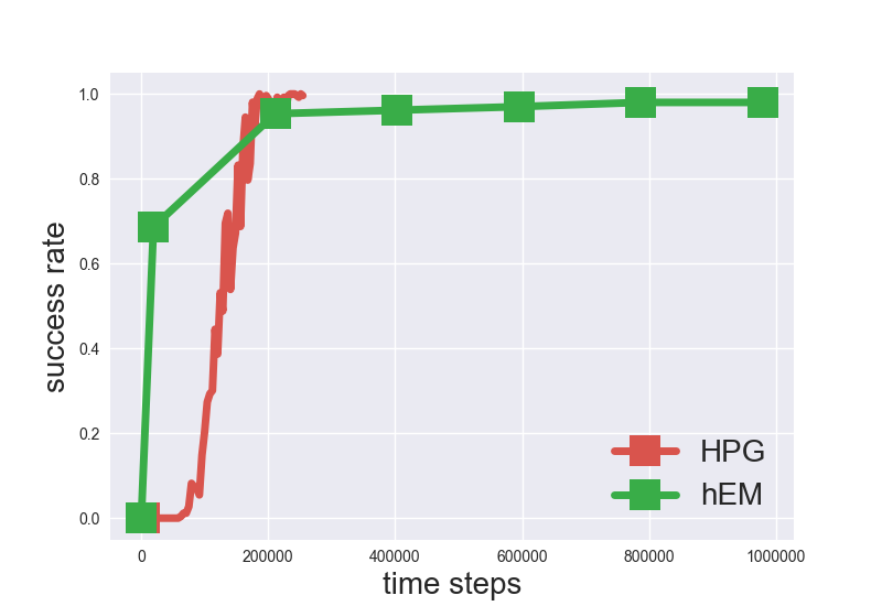
(a) Flip bit $K=25$

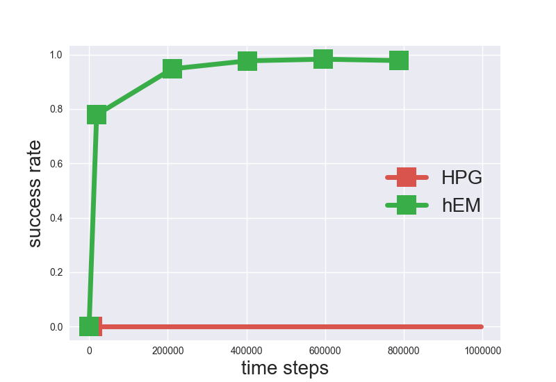
(b) Flip bit $K=50$

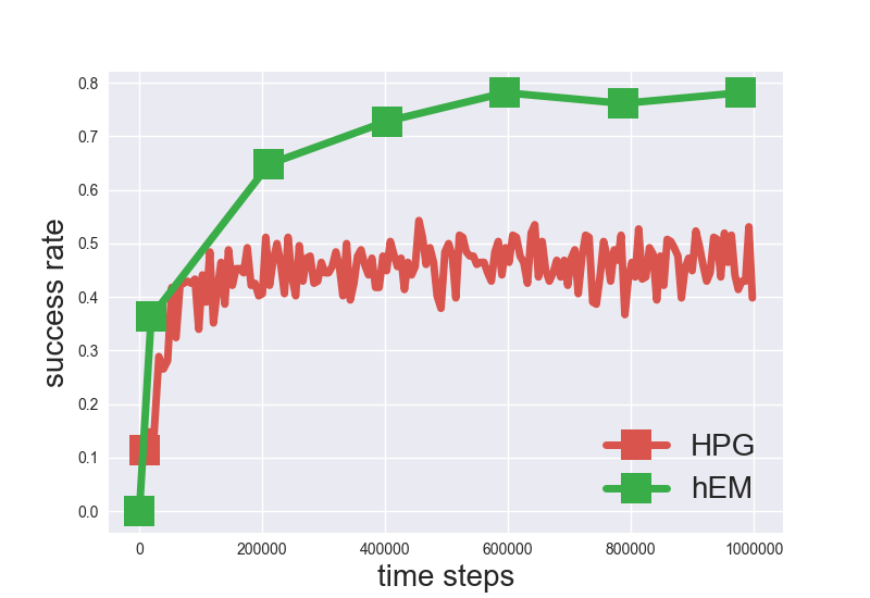
(c) Four room

Figure 11: Comparison between $\mathrm{h}$em and hpg. hpg performs well on Flip bit mdp with $K=25$, but when $K=50$ its performance drops drastically. hpg also underperforms $\mathrm{h}$em on the four room environment where it makes fast progress initially but saturates to a low sub-optimal level.

C.5 Additional Results on Baseline Fetch Tasks

Details on Fetch tasks.

Fetch tasks are introduced in [2]: Reach, Slide, Push and Pick and Place. We have already evaluated on the Reach task in our prior experiments. Here, we focus on the other three experiments.

Issues with exploration.

As we have alluded to in the main paper, exploration is a critical issue in goal-conditioned rl, as exemplified through the Fetch tasks. Compared to the reaching tasks we considered, Fetch tasks in general have more complicated goal space - purely random exploration might not cover the entire goal space fully. This observation has been corroborated in recent work [51, 52].

Details on algorithms.

To solve these tasks, we build on the built-in exploration mechanism of her implementations [61], which have been shown to work in certain setups. Though $\mathrm{h}$em does not utilize any value function critics, it shares the policy network with her. We implement the aggregate loss function as

$$L(\theta)=L_{\text{her}}+\eta\cdot L_{\text{hem}}= \mathbb{E}_{(s,g)\sim\mathcal{D}}\left[Q_{\phi}\left(s,\pi_{\theta}(s),g\right)\right]+\eta\cdot\mathbb{E}_{q(\tau,g)}\left[\sum_{t=0}^{T-1}\log\pi_{\theta}(a_{t}\mid s_{t},g)\right].$$

for the policy network. Here $\eta\in\{0.1,0.2,0.5\}$ is a hyper-parameter we selected manually to determine the trade-offs between two loss functions. Intuitively, when the policy cannot benefit from the learning signals of her via $L_{\text{her}}$, it is still able to learn via the supervised learning update through $L_{\text{hem}}$. In practice, we find $\eta=0.1$ works uniformly well.

Results.

See Figure 12 for the full results. Note that $\mathrm{h}$em provides marginal speed up on the learning on Push and Pick & Place. On Slide, both algorithms get stuck at local optimal (similar observations were made in [2]). We speculate that improvements in the exploration literature would bring further consistent performance gains.

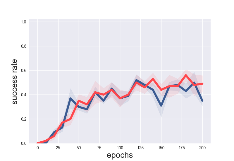
(a) Slide

(b) Push

(c) Pick and Place

Figure 12: Fetch tasks. Training curves of $\mathrm{h}$em and her on two standard Fetch tasks. $\mathrm{h}$em provides marginal speed up compared to her. All curves are calculated based on $5$ random seeds.

References

- [1] Andrew Y Ng, Daishi Harada, and Stuart Russell. Policy invariance under reward transformations: Theory and application to reward shaping. In ICML, volume 99, pages 278–287, 1999.
- [2] Marcin Andrychowicz, Filip Wolski, Alex Ray, Jonas Schneider, Rachel Fong, Peter Welinder, Bob McGrew, Josh Tobin, OpenAI Pieter Abbeel, and Wojciech Zaremba. Hindsight experience replay. In Advances in neural information processing systems, pages 5048–5058, 2017.
- [3] Volodymyr Mnih, Koray Kavukcuoglu, David Silver, Alex Graves, Ioannis Antonoglou, Daan Wierstra, and Martin Riedmiller. Playing atari with deep reinforcement learning. arXiv preprint arXiv:1312.5602, 2013.
- [4] Timothy P Lillicrap, Jonathan J Hunt, Alexander Pritzel, Nicolas Heess, Tom Erez, Yuval Tassa, David Silver, and Daan Wierstra. Continuous control with deep reinforcement learning. arXiv preprint arXiv:1509.02971, 2015.
- [5] Gerardo Rubino and Bruno Tuffin. Rare event simulation using Monte Carlo methods. John Wiley & Sons, 2009.
- [6] George Casella and Roger L Berger. Statistical inference, volume 2. Duxbury Pacific Grove, CA, 2002.
- [7] David M Blei, Alp Kucukelbir, and Jon D McAuliffe. Variational inference: A review for statisticians. Journal of the American Statistical Association, 112(518):859–877, 2017.
- [8] Alex X Lee, Anusha Nagabandi, Pieter Abbeel, and Sergey Levine. Stochastic latent actor-critic: Deep reinforcement learning with a latent variable model. arXiv preprint arXiv:1907.00953, 2019.
- [9] Ilya Kostrikov, Denis Yarats, and Rob Fergus. Image augmentation is all you need: Regularizing deep reinforcement learning from pixels. arXiv preprint arXiv:2004.13649, 2020.
- [10] Todd K Moon. The expectation-maximization algorithm. IEEE Signal processing magazine, 13(6):47–60, 1996.
- [11] Diederik P Kingma and Max Welling. Auto-encoding variational bayes. arXiv preprint arXiv:1312.6114, 2013.
- [12] Rajesh Ranganath, Sean Gerrish, and David M Blei. Black box variational inference. In Proceedings of the Seventeenth International Conference on Artificial Intelligence and Statistics, 2014.
- [13] Rudolf Kalman. On the general theory of control systems. IRE Transactions on Automatic Control, 4(3):110–110, 1959.
- [14] Emanuel Todorov. General duality between optimal control and estimation. In Decision and Control, 2008. CDC 2008. 47th IEEE Conference on, pages 4286–4292. IEEE, 2008.
- [15] Jens Kober and Jan R Peters. Policy search for motor primitives in robotics. In Advances in neural information processing systems, pages 849–856, 2009.
- [16] Sergey Levine and Vladlen Koltun. Variational policy search via trajectory optimization. In Advances in Neural Information Processing Systems, pages 207–215, 2013.
- [17] Abbas Abdolmaleki, Jost Tobias Springenberg, Yuval Tassa, Remi Munos, Nicolas Heess, and Martin Riedmiller. Maximum a posteriori policy optimisation. arXiv preprint arXiv:1806.06920, 2018.
- [18] H Francis Song, Abbas Abdolmaleki, Jost Tobias Springenberg, Aidan Clark, Hubert Soyer, Jack W Rae, Seb Noury, Arun Ahuja, Siqi Liu, Dhruva Tirumala, et al. V-mpo: On-policy maximum a posteriori policy optimization for discrete and continuous control. arXiv preprint arXiv:1909.12238, 2019.
- [19] Brian D Ziebart. Modeling purposeful adaptive behavior with the principle of maximum causal entropy. 2010.
- [20] Tuomas Haarnoja, Kristian Hartikainen, Pieter Abbeel, and Sergey Levine. Latent space policies for hierarchical reinforcement learning. arXiv preprint arXiv:1804.02808, 2018.
- [21] Sergey Levine. Reinforcement learning and control as probabilistic inference: Tutorial and review. arXiv preprint arXiv:1805.00909, 2018.
- [22] Jan Peters, Katharina Mulling, and Yasemin Altun. Relative entropy policy search. In Twenty-Fourth AAAI Conference on Artificial Intelligence, 2010.
- [23] Paulo Rauber, Avinash Ummadisingu, Filipe Mutz, and Juergen Schmidhuber. Hindsight policy gradients. arXiv preprint arXiv:1711.06006, 2017.
- [24] Ronald J Williams. Simple statistical gradient-following algorithms for connectionist reinforcement learning. In Reinforcement Learning, pages 5–32. Springer, 1992.
- [25] Richard S Sutton, David A McAllester, Satinder P Singh, and Yishay Mansour. Policy gradient methods for reinforcement learning with function approximation. In Advances in neural information processing systems, pages 1057–1063, 2000.
- [26] David Silver, Julian Schrittwieser, Karen Simonyan, Ioannis Antonoglou, Aja Huang, Arthur Guez, Thomas Hubert, Lucas Baker, Matthew Lai, Adrian Bolton, et al. Mastering the game of go without human knowledge. Nature, 550(7676):354–359, 2017.
- [27] Quan Vuong, Yiming Zhang, and Keith W Ross. Supervised policy update for deep reinforcement learning. arXiv preprint arXiv:1805.11706, 2018.
- [28] Julian Schrittwieser, Ioannis Antonoglou, Thomas Hubert, Karen Simonyan, Laurent Sifre, Simon Schmitt, Arthur Guez, Edward Lockhart, Demis Hassabis, Thore Graepel, et al. Mastering atari, go, chess and shogi by planning with a learned model. arXiv preprint arXiv:1911.08265, 2019.
- [29] Meire Fortunato, Mohammad Gheshlaghi Azar, Bilal Piot, Jacob Menick, Ian Osband, Alex Graves, Vlad Mnih, Remi Munos, Demis Hassabis, Olivier Pietquin, et al. Noisy networks for exploration. arXiv preprint arXiv:1706.10295, 2017.
- [30] Matthias Plappert, Rein Houthooft, Prafulla Dhariwal, Szymon Sidor, Richard Y Chen, Xi Chen, Tamim Asfour, Pieter Abbeel, and Marcin Andrychowicz. Parameter space noise for exploration. arXiv preprint arXiv:1706.01905, 2017.
- [31] Diederik P Kingma and Jimmy Ba. Adam: A method for stochastic optimization. arXiv preprint arXiv:1412.6980, 2014.
- [32] Yiming Ding, Carlos Florensa, Pieter Abbeel, and Mariano Phielipp. Goal-conditioned imitation learning. In Advances in Neural Information Processing Systems, pages 15298–15309, 2019.
- [33] Dibya Ghosh, Abhishek Gupta, Justin Fu, Ashwin Reddy, Coline Devin, Benjamin Eysenbach, and Sergey Levine. Learning to reach goals without reinforcement learning. arXiv preprint arXiv:1912.06088, 2019.
- [34] Benjamin Eysenbach, Xinyang Geng, Sergey Levine, and Ruslan Salakhutdinov. Rewriting history with inverse rl: Hindsight inference for policy improvement. arXiv preprint arXiv:2002.11089, 2020.
- [35] Junhyuk Oh, Yijie Guo, Satinder Singh, and Honglak Lee. Self-imitation learning. arXiv preprint arXiv:1806.05635, 2018.
- [36] Yijie Guo, Junhyuk Oh, Satinder Singh, and Honglak Lee. Generative adversarial self-imitation learning. arXiv preprint arXiv:1812.00950, 2018.
- [37] Yijie Guo, Jongwook Choi, Marcin Moczulski, Samy Bengio, Mohammad Norouzi, and Honglak Lee. Efficient exploration with self-imitation learning via trajectory-conditioned policy. arXiv preprint arXiv:1907.10247, 2019.
- [38] Yunhao Tang. Self-imitation learning via generalized lower bound q-learning. arXiv preprint arXiv:2006.07442, 2020.
- [39] Anirudh Goyal, Philemon Brakel, William Fedus, Soumye Singhal, Timothy Lillicrap, Sergey Levine, Hugo Larochelle, and Yoshua Bengio. Recall traces: Backtracking models for efficient reinforcement learning. arXiv preprint arXiv:1804.00379, 2018.
- [40] David Silver, Aja Huang, Chris J Maddison, Arthur Guez, Laurent Sifre, George Van Den Driessche, Julian Schrittwieser, Ioannis Antonoglou, Veda Panneershelvam, Marc Lanctot, et al. Mastering the game of go with deep neural networks and tree search. nature, 529(7587):484–489, 2016.
- [41] David Silver, Thomas Hubert, Julian Schrittwieser, Ioannis Antonoglou, Matthew Lai, Arthur Guez, Marc Lanctot, Laurent Sifre, Dharshan Kumaran, Thore Graepel, et al. A general reinforcement learning algorithm that masters chess, shogi, and go through self-play. Science, 362(6419):1140–1144, 2018.
- [42] Julian Schrittwieser, Ioannis Antonoglou, Thomas Hubert, Karen Simonyan, Laurent Sifre, Simon Schmitt, Arthur Guez, Edward Lockhart, Demis Hassabis, Thore Graepel, et al. Mastering atari, go, chess and shogi by planning with a learned model. Nature, 588(7839):604–609, 2020.
- [43] Jean-Bastien Grill, Florent Altché, Yunhao Tang, Thomas Hubert, Michal Valko, Ioannis Antonoglou, and Rémi Munos. Monte-carlo tree search as regularized policy optimization. In International Conference on Machine Learning, pages 3769–3778. PMLR, 2020.
- [44] Sergey Levine and Vladlen Koltun. Guided policy search. In International conference on machine learning, pages 1–9. PMLR, 2013.
- [45] Sergey Levine, Chelsea Finn, Trevor Darrell, and Pieter Abbeel. End-to-end training of deep visuomotor policies. The Journal of Machine Learning Research, 17(1):1334–1373, 2016.
- [46] Alexey Dosovitskiy and Vladlen Koltun. Learning to act by predicting the future. arXiv preprint arXiv:1611.01779, 2016.
- [47] Yuri Burda, Roger Grosse, and Ruslan Salakhutdinov. Importance weighted autoencoders. arXiv preprint arXiv:1509.00519, 2015.
- [48] Tom Rainforth, Adam R Kosiorek, Tuan Anh Le, Chris J Maddison, Maximilian Igl, Frank Wood, and Yee Whye Teh. Tighter variational bounds are not necessarily better. arXiv preprint arXiv:1802.04537, 2018.
- [49] Ashvin V Nair, Vitchyr Pong, Murtaza Dalal, Shikhar Bahl, Steven Lin, and Sergey Levine. Visual reinforcement learning with imagined goals. In Advances in Neural Information Processing Systems, pages 9191–9200, 2018.
- [50] Soroush Nasiriany, Vitchyr Pong, Steven Lin, and Sergey Levine. Planning with goal-conditioned policies. In Advances in Neural Information Processing Systems, pages 14814–14825, 2019.
- [51] Yunzhi Zhang, Pieter Abbeel, and Lerrel Pinto. Automatic curriculum learning through value disagreement. arXiv preprint arXiv:2006.09641, 2020.
- [52] Silviu Pitis, Harris Chan, Stephen Zhao, Bradly Stadie, and Jimmy Ba. Maximum entropy gain exploration for long horizon multi-goal reinforcement learning. arXiv preprint arXiv:2007.02832, 2020.
- [53] Tuomas Haarnoja, Aurick Zhou, Pieter Abbeel, and Sergey Levine. Soft actor-critic: Off-policy maximum entropy deep reinforcement learning with a stochastic actor. arXiv preprint arXiv:1801.01290, 2018.
- [54] Brian D Ziebart, Andrew L Maas, J Andrew Bagnell, and Anind K Dey. Maximum entropy inverse reinforcement learning. In Aaai, volume 8, pages 1433–1438. Chicago, IL, USA, 2008.
- [55] Roy Fox, Ari Pakman, and Naftali Tishby. Taming the noise in reinforcement learning via soft updates. arXiv preprint arXiv:1512.08562, 2015.
- [56] Kavosh Asadi and Michael L Littman. An alternative softmax operator for reinforcement learning. In Proceedings of the 34th International Conference on Machine Learning-Volume 70, pages 243–252. JMLR. org, 2017.
- [57] Michael C Fu. Stochastic gradient estimation. In Handbook of simulation optimization, pages 105–147. Springer, 2015.
- [58] Emanuel Todorov, Tom Erez, and Yuval Tassa. Mujoco: A physics engine for model-based control. In Intelligent Robots and Systems (IROS), 2012 IEEE/RSJ International Conference on, pages 5026–5033. IEEE, 2012.
- [59] Greg Brockman, Vicki Cheung, Ludwig Pettersson, Jonas Schneider, John Schulman, Jie Tang, and Wojciech Zaremba. Openai gym. arXiv preprint arXiv:1606.01540, 2016.
- [60] Tom Schaul, John Quan, Ioannis Antonoglou, and David Silver. Prioritized experience replay. arXiv preprint arXiv:1511.05952, 2015.
- [61] Prafulla Dhariwal, Christopher Hesse, Oleg Klimov, Alex Nichol, Matthias Plappert, Alec Radford, John Schulman, Szymon Sidor, and Yuhuai Wu. Openai baselines. https://github.com/openai/baselines, 2017.