Least action and the maximum-coupling approximations
in the theory of spontaneous fission

Abstract

We investigate the dynamics of spontaneous fission in a configuration-interaction (CI) approach. In that formalism the decay rate is governed by an effective interaction coupling the ground-state configuration and a fission doorway configuration, with the interaction strength determined by inverting a high-dimensioned CI Hamiltonian matrix that may have a block-tridiagonal structure. It is shown that the decay rate decreases exponentially with the number of blocks at a rate determined by the largest eigenvalue of a matrix in the block space for Hamiltonians with identical off-diagonal blocks. The theory is greatly simplified by approximations similar in spirit to the adiabatic and the least-action approximations in continuum representations. Here each block is replaced by a single matrix element. While the adiabatic reduction underestimates the coupling, a reduction based on a maximum-coupling approximation works well in a schematic CI model.

I Introduction

The theory of spontaneous fission is a challenging subject of multidimensional quantum tunneling. The theory is usually formulated by defining one or more collective coordinates in a constrained mean-field theory and then mapping the Hamiltonian or energy functional onto a Schrödinger equation in those coordinates. See for example Refs. Moller2009 ; Shunck2016 ; D19 ; whitepaper2020 . Once a tunneling path through the collective space is determined, the decay rate is calculated from the collective potential and inertia using the WKB formula.

The configuration interaction (CI) approach offers a completely different framework for calculating the large-amplitude dynamics needed in fission theory. Instead of invoking collective coordinates to describe the dynamics, the theory is based on the Hamiltonian interactions between configurations in a discrete basis. Not all of the tools for carrying out realistic calculations are presently in place, but several aspects have been demonstrated. In particular, one need not rely entirely on collective coordinates to construct the needed configuration spaces BM16 . Also, it is feasible to estimate the decay widths of doorway states into fission channels with available calculational tools BR19 . There are at least three advantages of the CI approach over the conventional approaches that can be mentioned. First, the overcompleteness problem inherent in the generator coordinate method (GCM) can be mitigated. Second, couplings to intrinsic excitations can be incorporated relatively easily. Finally, the Hamiltonian formulation is particularly suited for calculating fission cross sections in the $K$-matrix reaction theory Kawano15 ; Bertsch20 .

We have previously explored a schematic model based on the discrete basis approach, with application to induced fission Bertsch20 and to spontaneous fission HB20 . The Hamiltonian in the schematic model is simple enough to be fully solvable, so that it can serve as a test of existing approximations. One of the important findings in Ref. HB20 is that the adiabatic approximation, which is deeply embedded in the theory of spontaneous fission, may significantly underestimate the decay width. This has already been shown in realistic calculations in the WKB framework comparing the adiabatic treatment with the more sophisticated least-action approach Robledo14 ; Robledo18 ; Moretto74 . Clearly there is a need to understand the accuracy of the approximations inherent in the different approaches.

In this paper we propose a new approximation scheme within the CI framework, called here the “maximum-coupling approximation”. It has a close resemblance to the least-action approximation in the WKB formalism. Since the model is exactly solvable numerically, its accuracy can be tested. It was shown in the pioneering study of Moretto and Babinet Moretto74 that treating the pairing field as a dynamic variable strongly affects the calculated action in the tunneling region. This conclusion was recently re-affirmed by realistic calculations of the action using the generator coordinate method GCM Robledo14 ; Robledo18 . The same idea can be also implemented in the discrete-basis approach. This is done by increasing the pairing interaction to construct intermediate configurations at each shape parameter. As we will show, this approximation reproduces quite well the decay width that is obtained with the full Hamiltonian.

The paper is organized as follows. In Sec. II, we introduce the general framework for calculating transport in a CI basis, as well as the approximations and reductions made for dealing with large spaces. In Sec. III we apply the theory to the schematic model proposed in our earlier publications, comparing exact numerical calculations to approximate treatments including the maximum-coupling approximation. Finally in Sec. IV we discuss the relationship to the least-action approach.

II Discrete-basis approach

We assume that a basis of many-body states has been constructed BY19 ; BYR18 ; BYR19 to calculate the decay from a ground-state configuration through a doorway configuration for a particular decay channel. Because there is a large-amplitude reorganization of orbitals and occupation factors in the transition, many intermediate configurations must be included in the space.

II.1 Formulation

The general form of the Hamiltonian matrix is

$$\mbox{\bf H}=\left(\matrix{E_{g}&\mbox{\boldmath$v$}_{g}^{T}&0\cr\mbox{\boldmath$v$}_{g}&\mbox{\bf H}_{b}&\mbox{\boldmath$v$}_{d}\cr 0&\mbox{\boldmath$v$}_{d}^{T}&E_{d}\cr}\right),$$ (1)

in a notation using Roman boldface type font for matrices. $E_{g}$ and $E_{d}$ are the energies of the ground-state and doorway configurations, $\mbox{\bf H}_{b}$ (for “barrier”) is the Hamiltonian matrix of the intermediate configurations, and $\mbox{\boldmath$v$}_{g}$ and $\mbox{\boldmath$v$}_{d}$ are vector arrays of the matrix elements coupling $\mbox{\bf H}_{b}$ to the two end-point configurations. The energy of the doorway configuration has an imaginary part $\Gamma_{d}/2$, which may be evaluated with the Fermi golden rule as has been argued in Refs. BR19 ; BY19 . Notice that the introduction of a complex energy is equivalent to assuming a quasi-steady outgoing flow for the decay. The decay width can then be computed by diagonalizing the non-Hermitian H to find the imaginary part of the eigenenergy of the appropriate eigenfunction. However, the interpretation is complicated by the strong dependence of the decay width on the energy difference $E_{d}-E_{g}=\Delta-i\Gamma_{d}/2$. As was shown in Ref. HB20 , it is helpful to make an approximate reduction of H to an effective 2$\times$2 Hamiltonian matrix

$$\mbox{\bf H}_{\rm eff}=\left(\matrix{E_{g}&v_{\rm eff}\cr v_{\rm eff}&E_{g}+\Delta-i\Gamma_{d}/2\cr}\right),$$ (2)

where

$$v_{\rm eff}=\mbox{\boldmath$v$}_{g}\left[E_{g}\mathds{1}-\mbox{\bf H}_{b}\right]^{-1}\mbox{\boldmath$v$}^{T}_{d}.$$ (3)

Here $\mathds{1}$ is the unit matrix. This formulation also has the advantage that one avoids the computational issues associated with diagonalizing large non-Hermitian matrices. The coupling matrix element $v_{\rm eff}$ is generally small enough to be treated perturbatively, in which case the decay width $\Gamma_{f}$ is given by

$$\Gamma_{f}\approx\frac{\Gamma_{d}v_{\rm eff}^{2}}{\Delta^{2}+\Gamma_{d}^{2}/4}.$$ (4)

Thus the accuracy of approximations to $\left[E_{g}\mathds{1s}-\mbox{\bf H}_{b}\right]^{-1}$ can be assessed from comparing their derived $v_{\rm eff}$ values. The main calculational problem is inverting the large matrix in Eq. (3).

II.2 Large configuration spaces

The calculational problem of evaluating Eq. (3) can be simplified if the configurations in $\mbox{\bf H}_{b}$ can be ordered by some attribute such as the degree of elongation or the changes in orbital occupation numbers. Such configurations may be constructed e.g., in the Hartree-Fock approximation with a constraint on shape degrees of freedom BY19 ; BYR18 ; BYR19 . The configurations that are well separated in the ordered list are not directly connected by the Hamiltonian, and the matrix can therefore be considered to be block-tridiagonal,

$$\mbox{\bf H}_{b}\approx\left(\matrix{\mbox{\bf H}_{1}&\mbox{\bf V}_{1}&0&0&\cdots\cr\mbox{\bf V}_{1}^{T}&\mbox{\bf H}_{2}&\mbox{\bf V}_{2}&0&\cdots\cr 0&\mbox{\bf V}_{2}^{T}&\mbox{\bf H}_{3}&\mbox{\bf V}_{3}&\cdots\cr 0&0&\mbox{\bf V}_{3}^{T}&\mbox{\bf H}_{4}&\ddots\cr\vdots&\vdots&\vdots&\ddots&\ddots\cr}\right).$$ (5)

with $N_{b}$ blocks.

Similar Hamiltonians also occur in the theory of electron transport in carbon nanotubes Nardelli1999 and other structures Reuter11 , and the same calculational techniques can be applied here. As is well known, block tridiagonal matrices can be inverted by Gaussian elimination operating on the blocks rather the individual elements of the matrix (see Appendix). The block form of Gaussian elimination still requires inverting the diagonal block matrices, but their dimensions are much smaller when there are many blocks in $\mbox{\bf H}_{b}$. Further speedups are possible if the matrix has a block Toeplitz form Reuter11 ; Reuter12 ; hua97 . Later we will derive an asymptotic expression for the suppression of the tunneling rate as a function of the number of blocks in a block Toeplitz $\mbox{\bf H}_{b}$ of special form.

II.3 Adiabatic and maximum-coupling approximations

A very common approximation used in the WKB approach is the adiabatic treatment of the wave function under the barrier. The equivalent approximation in the CI approach is obtained by projecting the block matrices $\mbox{\bf H}_{n}$ onto the local ground state. To this end, we first diagonalize the $\mbox{\bf H}_{n}$ to find the local ground states,

$$\mbox{\bf H}_{n}\mbox{\boldmath$\psi$}^{({\rm ad})}_{n}=E_{n}^{({\rm ad})}\mbox{\boldmath$\psi$}^{({\rm ad})}_{n}.$$ (6)

Then we use the projection operators $P_{n}=|\mbox{\boldmath$\psi$}^{({\rm ad})}_{n}\rangle\langle\mbox{\boldmath$\psi$}^{({\rm ad})}_{n}|$ to reduce H to the $(N_{b}+2)$-dimensional matrix

$$\mbox{\bf H}_{\rm ad}=\left(\matrix{E_{g}&{v}_{g}&0&\cdots&0\cr{v}_{g}&E_{1}^{({\rm ad})}&{v}^{\rm ad}_{1}&\cdots&0\cr\vdots&\ddots&\ddots&\ddots&\vdots\cr 0&0&{v}^{\rm ad}_{N_{b}-1}&E_{N_{b}}^{({\rm ad})}&{v}_{d}\cr 0&0&0&{v}_{d}&E_{d}\cr}\right),$$ (7)

where $N_{b}$ is the number of blocks, and $v^{\rm ad}_{n}=\langle\mbox{\boldmath$\psi$}^{({\rm ad})}_{n}|\mbox{\bf V}_{n}|\mbox{\boldmath$\psi$}^{({\rm ad})}_{n+1}\rangle$, $v_{g}=\langle\phi_{g}|\mbox{\boldmath$v$}_{g}|\mbox{\boldmath$\psi$}^{({\rm ad})}_{n}\rangle$ and similarly for $v_{d}$.

As mentioned earlier, realistic calculations in the collective-coordinate approach have shown that the barrier penetration integral can be increased substantially by using wave functions that have stronger pairing condensates Robledo14-2 . The least-action approach chooses a pairing condensate having a strength that minimizes the action integral along the tunneling path. It was suggested in Ref. HB20 that the least-action treatment of the WKB penetrability could be simulated in the CI approach in a similar way, replacing the local ground-state wave functions used to construct $\mbox{\bf H}_{\rm ad}$ by wave functions that were more strongly paired. The maximum-coupling approximation is to choose the pairing strength which maximizes the derived $v_{\rm eff}$.

III Application to the schematic model

In this section we test various approximations with the schematic pairing-plus-quadrupole model introduced earlier Bertsch20 ; HB20 . For completeness, we first summarize details of the model as presented in those publications. The Fock-space Hamiltonian is defined as

$$\hat{H}=\sum_{k=0}^{N_{\rm orb}-1}\epsilon_{k}\hat{n}_{k}+v_{Q}\hat{Q}\hat{Q}-G\sum_{k\neq k^{\prime}}\hat{P}^{\dagger}_{k}\hat{P}_{k^{\prime}}$$ (8)

where $\hat{n}_{k}=a_{k}^{\dagger}a_{k}+a_{\bar{k}}^{\dagger}a_{\bar{k}}$ is the number operator for orbital $k$, $\hat{Q}=\sum_{k}q_{k}\hat{n}_{k}$ represents the quadrupole moment, and $\hat{P}_{k}=a_{k}^{\dagger}a_{\bar{k}}^{\dagger}$ is the pair creation operator.

The specific Hamiltonian treated numerically acts in a space of 6 doubly degenerate orbitals, $k=0,\cdots,5$, containing 6 paired particles, which we call the $(6,6)$ model. The single-particle energies are given by

$$\epsilon_{k}=(k~{}{\rm mod}~{}(N_{\rm orb}/2))\epsilon_{0},$$ (9)

where $\epsilon_{0}$ is the single-particle level spacing. The quadrupole moments are set to $q_{k}=(-1,-1,-1,1,1,1)$ for the six orbitals. The parameter $\epsilon_{0}$ sets the energy scale for the Hamiltonian. In terms of it, the other numerical parameters are chosen in the following way. We estimate $\epsilon_{0}$ at $Q=0$ using the Fermi gas approximation to obtain $\epsilon_{0}\sim 2/3$ MeV as a typical value for the actinide nuclei. The fission barrier height in the actinide region is $B\sim$ 6 MeV Vandenbosch73 , which is realized in the present (6,6) model with $v_{Q}=-13\epsilon_{0}/32$. The strength of the pairing gap is chosen to be $G=0.563\epsilon_{0}$ in order to reproduce $\Delta=1$ MeV in the BCS approximation with the single-particle spectrum of the $(6,6)$ model. These parameters are slightly different from those in Ref. HB20 , but we have confirmed that the conclusions in Ref.HB20 remain the same with the new parameter set.

The active model space includes only seniority-zero states, that is, configurations with 3 pairs in the 6 orbitals. There are four sets of configurations in the active space, distinguished by expectation values of the $\hat{Q}$ operator, $Q=-6,-2,2$, and 6. As indicated in Fig. 1, there is one configuration at $Q=-6$, the model ground state, and one configuration at $Q=+6$, which we take as the doorway state to fission. These two configurations are separated by a barrier formed by two blocks of configurations at $Q=\pm 2$. The resulting Hamiltonian has the form

$$\mbox{\bf H}=\left(\matrix{E_{g}&\mbox{\boldmath$v$}_{g}^{T}&0&0\cr\mbox{\boldmath$v$}_{g}&\mbox{\bf H}_{9}&\mbox{\bf V}_{9}&0\cr 0&\mbox{\bf V}_{9}&\mbox{\bf H}_{9}&\mbox{\boldmath$v$}_{g}\cr 0&0&\mbox{\boldmath$v$}_{g}^{T}&E_{g}\cr}\right).$$ (10)

Here $E_{g}$ is the energy of the ground state energy and $\mbox{\boldmath$v$}_{g}$ represents the coupling of the ground state and doorway to configurations in the barrier region. The blocks $\mbox{\bf H}_{9}$ and $\mbox{\bf V}_{9}$ are 9$\times$9 dimensional matrices. As in the previous section, we reduce the Hamiltonian to an effective 2$\times$2 matrix of the form Eq. (2). Its coupling matrix element is given by

$$v_{\rm eff}=(\mbox{\boldmath$v$}_{g}~{}0)\left[E_{g}\mathds{1}-\left(\matrix{\mbox{\bf H}_{9}&\mbox{\bf V}_{9}\cr\mbox{\bf V}_{9}&\mbox{\bf H}_{9}\cr}\right)\right]^{-1}\left(\matrix{0\cr\mbox{\boldmath$v$}_{g}\cr}\right).$$ (11)

The numerically exact value of $v_{\rm eff}$ for the assigned model parameters is given on the first line in Table I.

Table 1: Comparison of the adiabatic and maximum-coupling (MC) approximations to the exact coupling matrix element in the $(6,6)$ schematic model, as calculated by Eq. (11).

Model	$v_{\rm eff}$	$\left(v_{\rm eff}/v_{\rm eff}({\rm exact})\right)$
exact	0.0650
adiabatic	0.0221	0.34
MC	0.0653	1.00

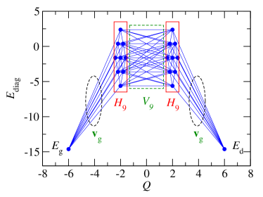
Figure 1: The model space for $(N_{\rm orb},N_{p})=(6,6)$ in the schematic discrete-basis model. The filled circles denote the diagonal energies, while the lines show the non-zero Hamiltonian matrix elements connecting configurations. The configurations contained in the interior diagonal blocks are enclosed in solid-line rectangles. The off-diagonal block $\mbox{\bf V}_{9}$ is indicated by the matrix elements passing through the dashed-line rectangle. Finally, the coupling vectors $\mbox{\boldmath$v$}_{g}$ and $\mbox{\boldmath$v$}_{d}$ are indicated by the matrix elements passing through the dashed-line ellipses.

III.1 Adiabatic approximation

The adiabatic approximation reduces the 20$\times$20 dimensional Hamiltonian to a 4$\times$4 matrix. The effective coupling in the further reduction to Eq. (2) is

$$v_{\rm eff}^{({\rm ad})}=\frac{v_{\rm ad}v_{g}^{2}}{\left(E_{b}^{({\rm ad})}\right)^{2}-v_{\rm ad}^{2}},$$ (12)

where $E_{b}^{({\rm ad})}=E_{0}^{({\rm ad})}-E_{g}$ is the adiabatic barrier height. The numerical value is shown on the second line of Table I. As we showed in Ref. HB20 , the adiabatic approximation considerably underestimates $v_{\rm eff}$ with the suppression factor $S\equiv(v_{\rm eff}^{({\rm ad})}/v_{\rm eff})^{2}$ of 0.116 with the present parameter set. A further calculation with a larger model spaces containing 3-4 internal blocks showed an even larger suppression factors.

III.2 Maximum coupling approximation

Guided by the findings in the collective-coordinate approach, we introduce the pairing condensate as a dynamical variable.

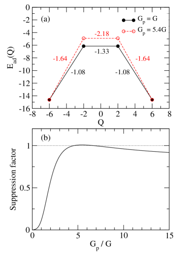
Figure 2: Panel a): comparison of energies and Hamiltonian matrix elements in the adiabatic approximation (the solid line with filled circles) to those obtained in the maximum-coupling approximation. (the dashed line with open circles). The numbers denote coupling strengths connecting the neighboring adiabatic states. Panel b): the suppression factor, $S(G_{p})\equiv(v_{\rm eff}^{({\rm ad})}(G_{p})/v_{\rm eff})^{2}$, as a function of $G_{p}/G$.

In the present approach, this corresponds to changing the ground state wave function in Eq. (6) to the lowest state of the block Hamiltonian having $G$ changed to $G_{p}$, that is, the solution to the eigenvalue equation

$$H_{9}(G_{p})|\phi^{({\rm ad})}_{0}(G_{p})\rangle=E_{0}^{({\rm ad})}(G_{p})|\phi^{({\rm ad})}_{0}(G_{p})\rangle.$$ (13)

The model Hamiltonian with the original $G$ is then diagonalized with the basis defined by $\phi^{({\rm ad})}_{0}(G_{p})$; the optimum pairing strength is the one giving the largest $v_{\rm eff}$. We call this the maximum-coupling approximation. The various matrix elements in the 4$\times$4 reduction are shown in the upper panel of Fig. 2. The solid line with filled circles show the interaction matrix element $v_{g},v_{d}$ and $v^{\rm ad}$ in the adiabatic approximation, that is, with $G_{p}=G$. The dashed line with open circles denotes the same quantities obtained with $G_{p}=5.4G$. Note that the fission barrier is higher, since the energy is not minimized. The increase of the barrier height is more than compensated for by the increase in $v_{g}$ and $v_{\rm ad}$. Fig. 2(b) shows the suppression factor, $S(G_{p})\equiv(v_{\rm eff}^{({\rm ad})}(G_{p})/v_{\rm eff})^{2}$, as a function of $G_{p}/G$. One can see that the suppression factor has a maximum near $G_{p}/G=5.4$, at which point the exact $v_{\rm eff}$ is well reproduced.

III.3 Block Toeplitz modeling

Realistic CI modeling of actinide nuclei might require of the order of $\sim$$20$ configuration sets to describe the physical barrier region (BYR19, , Fig.8). The $(6,6)$ model with its two sets is too oversimplified to simulate the behavior of long chains of intermediate configuration. However, we simulate the chains by replicating the $\mbox{\bf H}_{9}$ and $\mbox{\bf V}_{9}$ blocks along the diagonal and subdiagonals. The Hamiltonian is then characterized by the number $N_{b}$ of $\mbox{\bf H}_{9}$ blocks along the main diagonal. Such matrices are known as block Toeplitz matrices; as mentioned earlier there has been much effort in other fields to find efficient algorithms to invert them. It turns out that for the $(6,6)$ Hamiltonian one can extract the asymptotic dependence on $N_{b}$ from the properties of the eigenvalues of a matrix having the same dimension as $\mbox{\bf H}_{9}$.

Table 2: The effective coupling strength $v_{\rm eff}$ for the block tridiagonal matrix, Eq. (5), as a function of the number of blocks $N_{b}$. $\mbox{\bf H}_{9}$ and $\mbox{\bf V}_{9}$ are taken from the (6,6) model. The ratio to the effective strength for $N_{b}-1$ is also shown. The last row shows the ratio $e^{-\alpha}$ as computed from Eq. (21).

$N_{b}$	$v_{\rm eff}(N)$	$v_{\rm eff}(N_{b})/v_{\rm eff}(N_{b}-1)$
1	0.277	–
2	0.0650	0.2345
3	0.0154	0.2372
4	0.00367	0.2380
5	0.000875	0.2384
6	0.000209	0.2385
7	0.0000498	0.2386
8	0.0000119	0.2386
Eq. (21)		0.2386

First, we show in Table II the effective coupling strength $v_{\rm eff}$ as a function of $N_{b}$. See also Fig. 3. As is expected, $v_{\rm eff}$ decreases as $N_{b}$ increases. The Table and the figure also show the ratio of $v_{\rm eff}(N)$ to $v_{\rm eff}(N-1)$. One can see that the ratio goes asymptotically to a constant $C$ which we call the $N_{b}$-scaling factor,

$$C=\lim_{N\rightarrow\infty}v_{\rm eff}(N)/v_{\rm eff}(N-1)=0.2386.$$ (14)

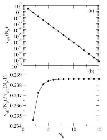
Figure 3: The effective coupling strength $v_{\rm eff}$ (the upper panel) and the ratio to the effective strength for $N_{b}-1$ (the lower panel) as a function of the number of blocks $N_{b}$.

A formula for $C$ can be derived as follows, assuming a Toeplitz structure of $H_{b}$ with symmetric $V_{T}$. We start with the equation for the wave function

$$\mbox{\bf H}\left(\matrix{\phi_{g}\cr\mbox{\boldmath$\psi$}\cr\phi_{d}\cr}\right)=E_{g}\left(\matrix{\phi_{g}\cr\mbox{\boldmath$\psi$}\cr\phi_{d}\cr}\right),$$ (15)

valid when $E_{d}=E_{g}$. Writing the $n$-th block component of the interior wave function as $\mbox{\boldmath$\psi$}_{n}$, each block row has the form

$$\mbox{\bf V}_{T}\mbox{\boldmath$\psi$}_{n-1}+\mbox{\bf H}_{T}\mbox{\boldmath$\psi$}_{n}+\mbox{\bf V}_{T}\mbox{\boldmath$\psi$}_{n+1}=E_{g}\mbox{\boldmath$\psi$}_{n}.$$ (16)

Note that $V_{9}^{T}=V_{9}\equiv V_{T}$ in this equation. Eq. (16) is invariant under translation of the block indices $n$. That implies that the wave function can be expressed as a sum over amplitudes that vary from block to block as $\mbox{\boldmath$\psi$}_{n+1}^{\lambda}=C_{\lambda}\mbox{\boldmath$\psi$}_{n}^{\lambda}$ where $C_{\lambda}$ is a constant. For tunneling under a barrier, $C_{\lambda}$ are all real and can be written as $C_{\lambda}=e^{\pm\alpha_{\lambda}}$. Substituting in Eq. (16) one obtains

$$(e^{\alpha_{\lambda}}+e^{-{\alpha_{\lambda}}})\mbox{\bf V}_{T}\mbox{\boldmath$\psi$}_{n}+(\mbox{\bf H}_{T}-E_{g}\mathds{1})\mbox{\boldmath$\psi$}_{n}=0.$$ (17)

This is equivalent to the eigenvalue equation

$$\left(-2(\mbox{\bf H}_{T}-E_{g}\mathds{1})^{-1}\mbox{\bf V}_{T}\right)\mbox{\boldmath$\psi$}_{n}=\lambda\mbox{\boldmath$\psi$}_{n}$$ (18)

with $\alpha_{\lambda}$ related to the eigenvalue by

$$\cosh(\alpha_{\lambda})=\lambda^{-1}.$$ (19)

The wave function will be decaying going from the ground state toward the doorway configuration so we may assume that the asymptotic behavior is

$$\mbox{\boldmath$\psi$}_{n+1}=e^{-\alpha_{\lambda}}\mbox{\boldmath$\psi$}_{n}$$ (20)

with $\alpha_{\lambda}>0$. Thus $v_{\rm eff}$ decreases when a block is added by

$$C=e^{-\alpha_{\lambda}}=e^{-\cosh^{-1}(|\lambda|)}$$ (21)

where $\lambda$ is the eigenvalue of Eq. (18) having the largest absolute value. Note that eigenvalues with $|\lambda|>1$ correspond to undamped propagation modes. If such eigenvalues are present, the physical conditions for barrier penetration are violated.

The last line in Table II shows the $N_{b}$-scaling factor $C$ derived from Eq. (21) for the $(6,6)$ model. The agreement with the observed reduction factor is excellent.

In a more general case with $V\neq V^{T}$, we have found two ways to compute $C$. One is somewhat parallel to the above argument, but starting from the block row equation

$$(\mbox{\bf V}_{T})^{T}\mbox{\boldmath$\psi$}_{n-1}+\mbox{\bf H}_{T}\mbox{\boldmath$\psi$}_{n}+\mbox{\bf V}_{T}\mbox{\boldmath$\psi$}_{n+1}=E_{g}\mbox{\boldmath$\psi$}_{n},$$ (22)

rather than Eq. (16). The other method is based on partial Gaussian elimination and is presented in the Appendix.

For the first method, we assume $\mbox{\boldmath$\psi$}_{n\pm 1}=e^{\mp\alpha}\mbox{\boldmath$\psi$}_{n}$ as in Eq. (17). Substituting in Eq. (22), one obtains

$$\left[(\mbox{\bf V}_{T})^{T}e^{\alpha}+\mbox{\bf H}_{T}-E_{g}\mathds{1}+\mbox{\bf V}_{T}e^{-\alpha}\right]\mbox{\boldmath$\psi$}_{n}\equiv M(\alpha)\mbox{\boldmath$\psi$}_{n}=0.$$ (23)

This equation is satisfied when the determinant of $M(\alpha)$ is zero. This can be solved numerically for $\alpha$, from which the $N_{b}$-scaling factor is evaluated as $C=e^{-\alpha}$.

We have verified that this method yields the same value of the $N_{b}$-scaling factor as that obtained with Eq. (21) when $\mbox{\bf V}=\mbox{\bf V}^{T}=\mbox{\bf V}_{9}$. Moreover, we have also confirmed that this method leads to the exact scaling factor when some of the components in $\mbox{\bf V}_{9}$ is set to be zero so that $\mbox{\bf V}_{9}\neq(\mbox{\bf V}_{9})^{T}$.

IV LINK TO LEAST ACTION APPROACH

IV.1 Derived action in the CI framework

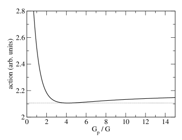
Figure 4: The local action $S\propto\sqrt{B/|v|}$ as a function of $G_{p}/G$. Here, the barrier height $B$ and the coupling strength $v$ are estimated with the lowest eigenstate of the intermediate Hamiltonian $H_{9}$ with a modification of the strength of the pairing interaction from $G$ to $G_{p}$.

The action integral in the collective-coordinate approach is given by

$$S=\int\left[\frac{2I(x)}{\hbar^{2}}(V(x)-E_{g})\right]^{1/2}dx;$$ (24)

where $I$ is the inertia of the system, often calculated in the Gaussian overlap approximation (R&S, , Sect. 10.7.4). The variable $x$ is a shape degree of freedom associated with the fission path, and $V(x)$ is the energy of the GCM configuration at the point $x$. We want to minimize $S$ given the $\mbox{\bf H}_{b}$ matrix of block Toeplitz form. We first reduce the matrix to the form

$$H_{b}=\left(\matrix{e&v&0&0\cdots&0\cr v&e&v&0\cdots&0\cr 0&v&e&v\cdots&0\cr\vdots&\vdots&\ddots&\ddots&\ddots\cr 0&0&0&v&e\cr}\right),$$ (25)

with the aid of a one-dimensional projection operator acting on the $H_{T}$ and $V_{T}$ matrices. The equation which corresponds to Eq. (16) then reads

$$v\psi_{n-1}+e\psi_{n}+v\psi_{n+1}=E_{g}\psi_{n}.$$ (26)

This is to be compared with a Schrödinger equation for a collective Hamiltonian,

$$\left(-\frac{\hbar^{2}}{2I}\frac{d^{2}}{dx^{2}}+V(x)\right)\phi(x)=E\psi(x).$$ (27)

Discretizing the differential operator as

$$\frac{d^{2}}{dx^{2}}\phi(x)\sim\frac{1}{(\Delta x)^{2}}\left[\psi(x_{n-1})-2\psi(x_{n})+\psi(x_{n+1})\right],$$ (28)

where $\Delta x$ is a mesh spacing of the variable $x$, the inertia parameter $I$ and the collective potential $V(x)$ can be read off as Barranco90

$$I = -\frac{\hbar^{2}}{2v}\frac{1}{(\Delta x)^{2}},$$ (29)

$$V(x) = e-2v.$$ (30)

Since the collective potential has a constant shift $-2v$ at all the points of $x$, we expect that the energy $E$ in Eq. (27) is approximately given by $E=E_{g}-2v$. Introducing exponentially decaying wave functions in Eq. (27),

$$\psi(x_{n-1})=e^{S\Delta x}\psi(x_{n}),~{}~{}~{}\psi(x_{n+1})=e^{-S\Delta x}\psi(x_{n}),$$ (31)

one obtains

$$\cosh(S\Delta x)=(IB(\Delta x)^{2}+1),$$ (32)

with $B\equiv e-E_{g}$. To be consistent with the discretization in Eq. (28), we expand the lefthand side of this equation to obtain

$$\cosh(S\Delta x)\sim 1+\frac{S(\Delta x)^{2}}{2}=(IB(\Delta x)^{2}+1),$$ (33)

from which the local action $S$ reads

$$S\sim\sqrt{2BI}$$ (34)

and its increment from block to block is

$$S\Delta x/\hbar=\sqrt{\left(\frac{B}{-v}\right)}.$$ (35)

Figure 2 shows the action as a function of $G_{p}/G$, where $B$ and $v$ are estimated with $\phi^{({\rm ad})}_{0}(G_{p})$ in Eq. (13). As in the maximum-coupling approximation discussed in Sec. II B, both $B$ and $|v|$ increase as a function of $G_{p}$, but the ratio has a minimum at some large value of $G_{p}$. With the parameter set which we employ for the (6,6) model, the minimum of the action is found at $G_{p}/G=4.1$. This is close to the value $G_{p}/G=5.4$ we obtained in the maximum-coupling approximation. In fact the suppression factor is not sensitive to the value of $G_{p}$ around the optimum value as may be seen in Fig. 2(b).

IV.2 Connection to the “number fluctuation”

In Refs. Robledo14 ; Robledo18 , the least-action formalism is applied by treating the number fluctuation as a collective variable in Hartree-Fock-Bogoliubov (HFB) wave functions. In terms of the HFB canonical variables $u_{k},v_{k}$, it is given by (R&S, , Eq. 6.44)

$$\Delta N^{2}=4\sum_{k>0}v_{k}^{2}u_{k}^{2}=4\sum_{k>0}v_{k}^{2}(1-v_{k}^{2}),$$ (36)

A related measure of the pairing strength is the abnormal density $\kappa$, defined for a $P^{\dagger}P$ pairing interaction as

$$\kappa=\sum_{k>0}u_{k}v_{k}=\sum_{k>0}v_{k}\sqrt{1-v_{k}^{2}}.$$ (37)

Since the CI approach is a number-conserving framework and has no number fluctuation, one cannot make a direct comparison to HFB pairing. But one can still make a connection through the orbital occupation numbers $n_{k}$ in the CI local ground state,

$$n_{k}=\langle\phi^{({\rm ad})}_{0}(G_{p})|a_{k}^{\dagger}a_{k}|\phi^{({\rm ad})}_{0}(G_{p})\rangle.$$ (38)

We make the identification $v_{k}^{2}=n_{k}$ to relate the CI wave function to the HFB quantities in Eq. (36) or (37). The result comes out to $\kappa=1.46$ and $\Delta N^{2}=1.50$ for the adiabatic wave function ($G_{p}=G$). Fig. 5 shows how the quantities relate to the action change with the two measures of pairing strength.

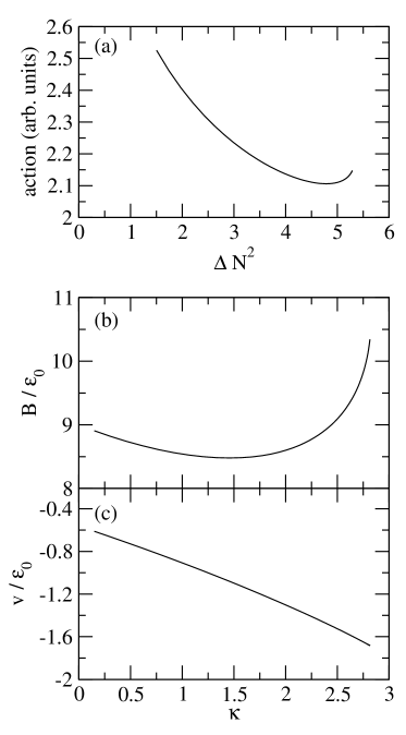
Figure 5: (The upper panel) The same as Fig. 4, but as a function of the number fluctuation $\Delta N^{2}$ defined by Eq. (36). (The middle and the bottom panels) The barrier height $B$ and the interaction $v$ as a function of the abnormal density defined by Eq. (37).

Fig. 5(a) shows the action increment Eq. (35) as a function of $\Delta N^{2}$. It decreases to 4.7 at $G_{p}=4.1G$ where it has a minimum. The ratio is 3.13, which is close to the ratio $\sim 3.17$ for ²³⁴U shown in Ref. Robledo14 . Figs. 5(b) and 5(c) show the barrier height $B$ and the interaction $v$ as a function of the pair density $\kappa$. These plots are shown to compare with the known small-amplitude behavior in BCS theory. There the leading behavior is $v\sim\kappa^{2}$ and $B\sim B^{\rm ad}+(\kappa-\kappa^{\rm ad})^{2}$ for B Moretto74 . A fit to these functional forms would be quite poor. But it might be that the validity of the quadratic formulas need a much larger orbital space than we have in the $(6,6)$ modeling.

V Summary

Using a schematic configuration-interaction model for spontaneous fission, we have investigated two approximations that go beyond the adiabatic approximation. To this end, we have constructed a single configuration at each shape by increasing the strength of the pairing interaction. This was motivated by the fact the pairing fluctuation makes an important degree of freedom in describing spontaneous fission based on the density functional approach. An increase of the pairing interaction results in an increase of both the barrier height and the coupling strength between neighboring configurations. In the first approximation, we investigated the maximum coupling approximation, in which the optimum value of the modified pairing strength is determined so that the effective coupling strength $v_{\rm eff}$ between the ground state and the fission doorway state is maximized. In this connection, we have investigated a chain of the interior matrix and have found that the effective coupling strength has a scaling property as a function of the number of blocks. We have shown that the scaling property can be understood by a simple eigenvalue equation if one assumes exponentially decaying wave functions for the fission degree of freedom.

In the second approximation, we have investigated the least action approach, in which the optimum value of the modified pairing strength is determined to minimize the action. This approximation can be derived in the context of the discrete basis model that we employ in this paper. We have shown that the optimum value of the modified pairing is close to that in the maximum-coupling approximation, yielding a reasonable value of the effective coupling strength. This gives some justification for treating the barrier penetration by the WKB formula with parameters derived from the CI approach.

In realistic applications to spontaneous fission, our studies with the schematic model have indicated that the adiabatic approximation can considerably underestimate the effective coupling strength, and thus the decay rate. The two approximations discussed in this paper, that is, the maximum-coupling approximation and the least action approach, provide a promising truncation scheme of configurations, by taking into account the non-adiabatic effects. The maximum-coupling approximation can be extended also to the case where the configurations are not orthogonal to each other Nardelli1999 ; Reuter11 . The main advantage of the CI approach is that it permits much richer configuration spaces than can be easily achieved with the GCM or pure mean-field dynamics. However, as mentioned earlier, new computation tools need to be developed for constructing the spaces and especially for calculating Hamiltonian matrix elements between arbitrary configurations.

Appendix A Block scaling factor from the Gaussian elimination method

For a block-tridiagonal matrix (5), the Greens function $G=\left[\mbox{\bf H}_{b}-E_{g}\mathds{1}\right]^{-1}$ has a form of

$$\mbox{\bf G}=\left(\matrix{\mbox{\bf G}_{11}&\cdots&\mbox{\bf G}_{1N}\cr\vdots&\ddots&\vdots\cr\mbox{\bf G}_{N1}&\cdots&\mbox{\bf G}_{NN}\cr}\right).$$ (39)

Here the subscript $b$ in the number of blocks $N_{b}$ has been dropped for clarity. In this notation the effective coupling (3) is given by

$$v_{\rm eff}=-\mbox{\boldmath$v$}_{g}^{T}\mbox{\bf G}_{1N}\mbox{\boldmath$v$}_{d}.$$ (40)

The matrix $\mbox{\bf G}_{1N}$ can be computed by a partial block-wise Gaussian elimination Nardelli1999 ; Reuter11 ; Reuter12 ; Hod06 . In this method, one first generates matrices $\mbox{\bf A}_{n}$ by iterating

$$\mbox{\bf A}_{n}=\mbox{\bf V}_{n-1}^{T}(\tilde{\mbox{\bf H}}_{n-1}-\mbox{\bf A}_{n-1})^{-1}\mbox{\bf V}_{n-1},~{}~{}~{}~{}(n=2,3,\cdots,N),$$ (41)

starting from $\mbox{\bf A}_{1}=0$. Here, $\tilde{\mbox{\bf H}}_{n}$ is defined as $\tilde{\mbox{\bf H}}_{n}\equiv\mbox{\bf H}_{n}-E_{g}\mathds{1}$. We assume all blocks have the dimension, so A matrices are square and of the same dimension. The $(N,N)$ component of the Greens function $\mbox{\bf G}_{NN}$ is given by

$$\mbox{\bf G}_{NN}=(\tilde{\mbox{\bf H}}_{N}-\mbox{\bf A}_{N})^{-1}$$ (42)

The Greens function component $\mbox{\bf G}_{1N}$ in Eq. (40) can be obtained recursively as

$$\mbox{\bf G}_{n,N}=-(\tilde{\mbox{\bf H}}_{n}-\mbox{\bf A}_{n})^{-1}\mbox{\bf V}_{n}\mbox{\bf G}_{n+1,N},~{}~{}~{}(n=N-1,\cdots,1).$$ (43)

For our purposes, we do not need the Greens function itself but only the $N_{b}$-scaling factor relating $\mbox{\bf G}_{1,N}$ and $\mbox{\bf G}_{1,N-1}$. From the algebraic structure of the Gaussian elimination quantities it is easy to show that the relationship can be expressed

$$\mbox{\bf G}_{1N}(N) = -\mbox{\bf G}_{1,N-1}(N-1)\mbox{\bf V}_{N-1}\mbox{\bf G}_{NN}(N),$$

$$= -\mbox{\bf G}_{1,N-1}(N-1)\mbox{\bf V}_{N-1}(\tilde{\mbox{\bf H}}_{N}-\mbox{\bf A}_{N})^{-1}.$$

Note that the effective interaction is given by $v_{\rm eff}(N)=-\mbox{\boldmath$v$}_{g}^{T}\mbox{\bf G}_{1N}(N)\mbox{\boldmath$v$}_{d}$ and $v_{\rm eff}(N-1)=-\mbox{\boldmath$v$}_{g}^{T}\mbox{\bf G}_{1,N-1}(N-1)\mbox{\boldmath$v$}_{d}$.

For a block Toeplitz matrix with $\mbox{\bf V}_{n}=\mbox{\bf V}_{T}$ and $\tilde{\mbox{\bf H}}_{n}=\mbox{\bf H}_{T}$, one may expect that Eq. (41) produces a sequence that converges to a fixed $\mbox{\bf A}\equiv\mbox{\bf A}_{\infty}$ as $N\rightarrow\infty$. In this limit, $\mbox{\bf G}_{NN}\rightarrow(\mbox{\bf H}_{T}-\mbox{\bf A}_{\infty})^{-1}\equiv\mbox{\bf G}_{\infty}$. When this is realized, one may also assume that the $N_{b}$-scaling factor $C$ can be computed from

$$\mbox{\bf G}_{1N}(N)=C\mbox{\bf G}_{1,N-1}(N-1).$$ (46)

Substituting this to Eq. (A), one finds that $C$ may be calculated as $C=\lambda_{\rm max}$, where $\lambda_{\rm max}$ is the largest eigenvalue of $-\mbox{\bf V}_{T}\mbox{\bf G}_{\infty}$. Note that the iterations in Eq. (41) need not be extend to $n=N$ if the asymptotic form of $\mbox{\bf A}_{n}$ is approached with fewer iterations.

Table 3: The $N_{b}$-scaling factor corresponding to Table II, but obtained with the Gaussian elimination method. In this method, the scaling factor is given by $\lambda_{\rm max}(n)$, that is, the largest eigenvalue of $-\mbox{\bf V}_{T}(\mbox{\bf H}_{T}-\mbox{\bf A}_{n})^{-1}$, where the matrix $\mbox{\bf A}_{n}$ is given by Eq. (41). The table shows this quantity as a function of $n$.

$n$	$\lambda_{\rm max}(n)$
1	0.22576
2	0.23788
3	0.23857
4	0.23861
5	0.23861
6	0.23861
7	0.23861
8	0.23861
9	0.23861
10	0.23861

Table III shows $\lambda_{\rm max}(n)$, that is, the largest eigenvalue of $-\mbox{\bf V}_{T}(\mbox{\bf H}_{T}-\mbox{\bf A}_{n})^{-1}$, as a function of $n$. One can first see that the asymptotic value of this quantity coincides with the $N_{b}$-scaling factor shown in Table II. Secondly, one can see that after a few iterationcs $\lambda_{\rm max}(n)$ quickly converges to the asymptotic value. This implies that $\mbox{\bf G}_{NN}(N)=(\mbox{\bf H}_{T}-\mbox{\bf A}_{N})^{-1}$ can be estimated as $\mbox{\bf G}_{NN}(N)\sim\mbox{\bf G}_{nn}(n)=(\mbox{\bf H}_{T}-\mbox{\bf A}_{n})^{-1}$ with a much smaller value of $n$ compared to the actual $N$.

References

- (1) P. Möller, A.J. Sierk, T. Ichikawa, A. Iwamoto, R. Bengtsson, H. Uhrenholt, and S. Åberg, Phys. Rev. C79, 064304 (2009).
- (2) N. Schunck and L.M. Robledo, Rep. Prog. Phys. 79, 116301 (2016).
- (3) J. Dobaczewski, arXiv:1910.03924 (2019).
- (4) M. Bender et al., arXiv:2005.10216 (2020).
- (5) G.F. Bertsch and J.M. Mehlhaff, EPJ Web of Conf. 122, 01001 (2016).
- (6) G.F. Bertsch and L.M. Robledo, Phys. Rev. C100, 044606 (2019).
- (7) T. Kawano, P. Talou, and H.A. Weidenmüller, Phys. Rev. C92, 044617 (2015).
- (8) G.F. Bertsch, Phys. Rev. C101, 034617 (2020).
- (9) K. Hagino and G.F. Bertsch, Phys. Rev. C, in press. arXiv:2003.03702 (2020).
- (10) S.A. Giuliani, L.M. Robledo, and R. Rodríguez-Guzmán, Phys. Rev. C90, 054311 (2014).
- (11) R. Rodríguez-Guzmán and L.M. Robledo, Phys. Rev. C98, 034308 (2018).
- (12) L.G. Moretto and R.P. Babinet, Phys. Lett. 49B, 147 (1974).
- (13) G.F. Bertsch and W. Younes, Ann. of Phys. (N.Y.) 403, 68 (2019).
- (14) G.F. Bertsch, W. Younes, and L.M. Robledo, Phys. Rev. C97, 064619 (2018).
- (15) G.F. Bertsch, W. Younes, and L.M. Robledo, Phys. Rev. C100, 024607 (2019).
- (16) M.B. Nardelli, Phys. Rev. B60, 7828 (1999).
- (17) M.G. Reuter, T. Seideman, and M.A. Ratner, Phys. Rev. B83, 085412 (2011).
- (18) M.G. Reuter and J.C. Hill, Comp. Sci. Discovery 5, 014009 (2012).
- (19) Y. Huang and W.F. McColl, J. Phys. A, 30 7919 (1997).
- (20) R. Rodríguez-Guzmán and L.M. Robledo, Phys. Rev. C89, 054310 (2014).
- (21) R. Vandenbosch and J.R. Huizenga, Nuclear Fission (Academic Press, 1973).
- (22) P. Ring and P. Schuck, The Nuclear Many-Body Problem (Springer, New York, 1980).
- (23) F. Barranco, G.F. Bertsch, R.A. Broglia, and E. Vigezzi, Nucl. Phys. A512, 253 (1990).
- (24) O. Hod, J.E. Peralta, and G.E. Scuseria, J. Chem. Phys. 125, 114704 (2006).
- (25) N.M. Boffi, J.C. Hill, and M.G. Reuter, Comp. Sci. Discovery 8, 015001 (2015).