Generalizing Gain Penalization for Feature Selection in Tree-based Models

Abstract

We develop a new approach for feature selection via gain penalization in tree-based models. First, we show that previous methods do not perform sufficient regularization and often exhibit sub-optimal out-of-sample performance, especially when correlated features are present. Instead, we develop a new gain penalization idea that exhibits a general local-global regularization for tree-based models. The new method allows for more flexibility in the choice of feature-specific importance weights. We validate our method on both simulated and real data and implement it as an extension of the popular R package ranger.

1 Introduction

In many Machine Learning problems, features can be hard or economically expensive to obtain, and some may be irrelevant or poorly linked to the target. For these reasons, reducing the number of features is an important task when building a model, and benefits the data visualization and model performance, whilst reducing storage and training time requirements [23]. However, for tree-based methods, there is no standard procedure for feature selection or regularization in the literature, as one would find for Linear Regression and the LASSO [47] for example. Performing feature selection in trees can be difficult, as they struggle to detect highly correlated features and their feature importance measures are not fully trustworthy [30]. Several methods to tackle this problem have been recently proposed, including Diaz-Uriarte [18], Friedman & Popescu [20], and Deng & Runger [15].

In Friedman & Popescu [20], the authors treat trees as parametric models and use procedures analogous to LASSO-type shrinkage methods, by penalizing the coefficients of the base learners and reducing the redundancy in each path from the root node to a leaf node. However, their selected features can still be redundant, since the focus is on reducing the number of rules instead of the number of features. Diaz-Uriarte [18] focuses on gene selection for classification. The authors propose an iterative tool that eliminates the least important features (in fractions of the number of features, $p$) and updates the algorithm at each iteration. The complication is that the method will always be either computationally expensive, if $p$ is low, or will eliminate too many features at once, which can exclude useful or interaction features. Besides, the method does not generalize to other dataset contexts or tasks, such as regression. In the contrasting approach of Deng & Runger [15, 16], the authors regularize Random Forests by gain penalization. Their method consists of letting the features only be picked by a Random Forest if their penalized (weighted) gain is still high. They make recommendations on how to set the penalization coefficients and present their implementation in the RRF package for R [rmanual]. However, the authors give no further guidelines on how to generalize their method for other models and penalization types and do not explore the influence of hyperparameters on the algorithm.

We develop a gain penalization approach that is more general and widely applicable than those mentioned above. In particular, our contributions are:

• We provide a richer means by which local and global regularization of features can be balanced and allow for bespoke local regularization functions for domain-specific applications.

• We generalize gain penalization to multiple tree-based methods (CART, Bagging, Random Forests), for both regression and classification.

• We propose different techniques for setting the regularization parameters and discuss how they affect the final results, with real and simulated examples.

• We make available a faster implementation of the regularization method, included in the very widely used ranger package.

The paper is structured as follows. Section 2 explains the problem setup, followed by the generalization of gain penalization in Section 3. In Section 4, we present the results for simulated and real data. Section 5 explains the implementation details, and Section 6 has the conclusions and future work.

2 Problem setup

Consider a set of training target-feature pairs $(Y_{i},\mathbf{x}_{i})\in\mathbb{R}\times\mathbb{R}^{p}$, with $i=1,\dots,N$ indexing the observations with $p$ being the total number of features. In general, we can estimate an $\hat{f}$ that describes how the features $\mathbf{x}_{i}$ relate to $Y_{i}$ and use it for prediction or inference. However, not all features need to be involved in $\hat{f}$. Especially for tree-based models, the occurrence of noisy or correlated features can badly influence the results [46]. Our interest here relies on estimating $\hat{f}$ such that it will only use the matrix $\mathbf{x}_{A}$, composed by the sub-vectors of $\mathbf{x}\in\mathbb{R}^{p}$ indexed by $A$, $A\subset\{1,\dots p\}$, which should contain the optimal set of features (it produces similar or equal prediction errors as the full matrix of features), that is potentially of a much smaller dimension.

2.1 Trees

Trees are a particular case of non-linear models, that recursively partition the feature space, resulting in a local model for each estimated region [8]. They learn the features directly from the training data, creating an adaptive basis function model (ABM) [31] of the form

$$f(\mathbf{x})=\mathbb{E}[y\mid\mathbf{x}]=\sum_{r=1}^{R}w_{r}\mathbb{I}(\mathbf{x}\in R_{r})=\sum_{r=1}^{R}w_{r}\phi_{r}(\mathbf{x};\mathbf{v}_{r}),$$ (1)

where $R_{r}$ is the $r$-th region, $w_{r}$ is the prediction given to this region and $\mathbf{v}_{r}$ represents the splitting feature chosen to and the correspondent splitting value. These algorithms are fitted using a greedy procedure, that computes a locally optimal maximum likelihood estimator by finding the splits that lead to the minimization of a cost function. For regression, the cost function of a decision $\mathbb{D}$ is frequently defined as $cost(\mathbb{D})=\sum_{i\in\mathbb{D}}(y_{i}-\bar{y})^{2}$, where $\bar{y}=(\sum_{i\in\mathbb{D}}y_{i})|\mathbb{D}|^{-1}$ is the mean of the observations in the specified region, while for classification this function is replaced by the misclassification rate, or $cost(\mathbb{D})=|\mathbb{D}|^{-1}\sum_{i\in\mathbb{D}}\mathbb{I}(y_{i}\neq\hat{y})$. The gain of a new split is a normalized measure of the cost reduction, given by

$$\begin{split}\Delta(i,t)=&cost(\mathbb{D})-\left(\frac{|\mathbb{D}_{LN_{(i,t)}}|}{|\mathbb{D}|}cost(\mathbb{D}_{LN_{(i,t)}})+\frac{|\mathbb{D}_{RN_{(i,t)}}|}{|\mathbb{D}|}cost(\mathbb{D}_{RN_{(i,t)}})\right),\end{split}$$ (2)

for feature $i$ at splitting point $t$, while $\mathbb{D}$ is related to the previous estimated split, $LN=\text{(left candidate node)}$ and $RN=\text{(right candidate node)}$. The global importance value is given by accumulating the gain over a feature, $\Delta(i)=\sum_{t\in\mathbb{S}_{i}}\Delta(i,t)$, where $\mathbb{S}_{i}$ now represents all the splitting points used in a tree for the $i-$th feature.

2.2 Ensembles

Trees are known to be high variance estimators: small changes in the data can lead to the estimation of a completely different tree [31]. One way to increase stability is to use the property that an average of many estimates has a smaller variance than one estimate, and grow many trees from re-samples of the data. Averaging such results give us a bagged ensemble [5] of the form $\hat{f}(\mathbf{x})=\sum_{n=1}^{N_{tree}}\frac{1}{N_{tree}}\hat{f}_{n}(\mathbf{x}),$ where $\hat{f}_{n}$ corresponds to the $n$-th tree. The Random Forest [6] algorithm is defined by allowing only a random subset $m$ of the features to be the candidates in each split. For ensembles, the importance value for a feature gets averaged over all the trees, or

$$Imp_{i}=\frac{1}{N_{tree}}\sum_{n=1}^{N_{tree}}\Delta(i)_{n},$$ (3)

for feature $i$. Moreover, the performance of the trees in a Random Forest relies on the number of features tried at each split, called mtry here, as when $\texttt{mtry}\rightarrow 1$, the larger the variance of each tree, but the more effective will be the averaging process, and vice versa [30].

2.3 Regularization by gain penalization

In Deng & Runger [15], the authors first discuss the regularization of Random Forests by gain penalization. The Regularized Random Forest (RRF) proposes weighting the gains of the splits during the greedy procedure, guiding the feature choosing of the model. The regularized gain is defined as

$$\text{Gain}_{R}(\mathbf{X}_{i},t)=\begin{cases}\lambda_{i}\Delta(i,t),\thinspace i\notin\mathbb{U}\text{ and}\\ \Delta(i,t),\thinspace i\in\mathbb{U},\end{cases}$$ (4)

where $\mathbb{U}$ is the set of indices of the features previously used, $\mathbf{X}_{i}$ is the candidate feature, and $t$ the candidate splitting point. The $\lambda_{i}\in(0,1]$ parameter is the penalty coefficient that controls the amount of regularization each feature receives. A feature is penalized if it is new to the whole ensemble, as the method has a memory of which features were already used. Naturally, $\lambda_{i}$ can be a constant value for all the features but ideally, there should be a regularization parameter for each feature that best represents the information they carry about the target. In Deng & Runger [16], the authors develop this idea by introducing the Guided RRF. It consists of first running a Standard Random Forest (mtry $\approx\sqrt{p}$, number of trees = 500), producing an importance measure for each feature and scaling this measure, in order to find $Imp_{i}^{{}^{\prime}}=\frac{Imp_{i}}{max_{j=1}^{P}Imp_{j}}$, where $Imp_{i}$ is the importance measure calculated for the $i$-th feature in the Random Forest. The estimated normalized variable importance measures are considered jointly with a regularization parameter to create the overall gain penalization.

3 Generalizing Gain Penalization

One of our goals with this work is to show how Equation 4 can be fully generalized in two senses: in the algorithm type and the penalization coefficients. For the algorithm, this means that the regularization method can be applied to any tree-based model (single trees such as CART or ensembles). As for the penalization coefficients, we generalize the method by proposing that $\lambda_{i}$ can be written as

$$\lambda_{i}=(1-\gamma)\lambda_{0}+\gamma g(\mathbf{x}_{i}),$$ (5)

where $\lambda_{0}\in[0,1)$ is interpreted as the baseline regularization, $g(\mathbf{x}_{i})$ is a function of the $i$-th feature, and $\gamma\in[0,1)$ is their mixture parameter, with $\lambda_{i}\in[0,1)$. The equation balances how much all features should be jointly, or globally, penalized and how much will it be due to a local $g(\mathbf{x}_{i})$. When $\gamma=0$, we return to what was proposed in Deng & Runger [15], and for $\gamma=1$, the regularization is fully controlled by $g(\mathbf{x}_{i})$. The $g(\mathbf{x}_{i})$ should represent relevant information about the features, based on some characteristic of interest. It can include, for example, external information about the relationship between $\mathbf{x}_{i}$ and $\mathbf{y}$, thus this has inspiration on the use of priors made in Bayesian methods. In the same fashion, the data will tell us how strong our assumptions about the penalization are, since even if we try to penalize a truly important feature, its gain will be high enough to overcome the penalization and the feature will get picked.

3.1 Choosing $g(\mathbf{x}_{i})$

Correlation: A natural option for continuous features is just to use $g(\mathbf{x}_{i})$ as the absolute value of the marginal correlation between $\mathbf{x}_{i}$ and $\mathbf{y}$, assuming a continuous target problem. It can be Pearson’s, Kendall’s, Spearman’s, or other correlation coefficient of preference (the first is more suitable for ordinary numeric inputs, while the others will be more convenient for ordered inputs [9]). We can define it as $g(\mathbf{x}_{i})=|corr(\mathbf{y},\mathbf{x}_{i})|$.

Entropy and Mutual Information: A different situation is when the features are discrete. In information theory, Shannon’s entropy [43] is a measure of the uncertainty of a (discrete) random feature. In short, if a discrete feature $X$ has $K$ states, its entropy will be calculated as $\mathbb{H}(X)=-\sum_{k=1}^{K}p(X=k)\log_{2}p(X=k),$ where $\mathbb{H}(X)\in[0,\infty]$. Higher entropy will mean more uncertainty, so it is reasonable to give more weight to features with lower uncertainties. One can use a normalized version of the entropy calculated for each $\mathbf{x}_{i}$, or $g(\mathbf{x}_{i})=1-\frac{\mathbb{H}(\mathbf{x}_{i})}{max_{j=1}^{P}\mathbb{H}(\mathbf{x}_{j})},$

compelling the features with lower entropy to have larger penalization coefficients. Similarly, we can also use the Mutual Information function, for which the similarity between a joint distribution $p(X,Y)$ and a factored distribution $p(X)p(Y)$ and we calculate $\text{MutInf}(X;Y)=\sum_{x}\sum_{y}p(x,y)\log\frac{p(x,y)}{p(x)p(y)}$ for two features $X$ and $Y$ [31]. Recalling the Entropy equation, it is easy to see that the Mutual Information value is the reduction in the uncertainty about $Y$ when we observe $X$, so it can be straightforwardly used as $g(\mathbf{x}_{i})=\frac{\text{MutInf}(\mathbf{x}_{i},\mathbf{y})}{max_{j=1}^{P}\text{MutInf}(\mathbf{x}_{j},\mathbf{y})}$.

Boosted: When there is no interest in differentiating continuous or discrete features, one can use a Boosted $g(\mathbf{x}_{i})$. Such functions depend on previously run machine learning models that provide an importance value for the features. The term Boosted is to introduce some familiarity, since we can arguably see the algorithm as an heterogenous Boosting [34] applied to the features instead of the observations. Examples of Machine Learning algorithms that allow for the calculation of an importance value include: tree ensembles, Generalized Linear Models [35], where the normalized absolute parameter coefficients can be interpreted as importance values, and Support Vector Machines [25] that produce importance values via sensitivity analysis [13, 12]. We should note that each family of algorithms will have its specific characteristics and preferences towards the features, that might need to be taken into account.

Combination: Another possibility is combining two or more $g(\mathbf{x}_{i})$. Objectively speaking, some functions will be more appropriate to one type of feature than others. As an example, one could combine a Boosted method with the marginal correlations between the target and each feature, letting the absolute values of the correlations compose $g(\mathbf{x}_{i})$ if the correlation is over a certain threshold $\epsilon$, and use $Imp_{i}^{{}^{\prime}}$ from a previously run algorithm otherwise.

Depth parameter: Growing very bushy trees with new features is not desirable when we want to use a small set of features. Following Chipman et al. [10], where the authors use prior distributions for whether a new feature should be picked in a Bayesian Regression Tree, we introduce the idea of increasing the penalization given the current depth of the tree. Their priors take into account the current depth of a tree, so when a tree is already deep the priors get less concentrated in high probability regions, resulting in lesser bushier trees. In our work, a similar idea is applied by setting

$$Gain_{R}(\mathbf{X}_{i},t,\mathbb{T})=\begin{cases}\lambda_{i}^{d_{\mathbb{T}}}\Delta(i,t),\thinspace i\notin\mathbb{U}\text{ and}\\ \Delta(i,t),\thinspace i\in\mathbb{U},\end{cases}$$ (6)

where $d_{\mathbb{T}}$ is the current depth of the $\mathbb{T}$ tree, $\mathbb{T}=(1,\dots,\texttt{ntree})$, for the $i$-th feature. The aim here is to reduce the gains of the features if they are to be picked in a deep node, preventing new features to appear at the bottom of trees unless their gains are exceptionally high.

3.2 Issues & Details

Feature masking effect: Tree-based models often suffer from feature masking effects (Louppe [30]). For example, in a tree, some feature $X_{j}$ might never occur in the algorithm if it leads to splits slightly worse than some other feature $X_{i}$, so if $X_{i}$ is removed, $X_{j}$ can prominently occur. This should be overcomed by ensembles like Random Forests, as selecting only $m$ features to pick from decorrelates the trees, but if we regularize the Random Forests, the problem remains. If weak features end up being first picked by the model, their gains will have an unfair advantage against the other features, which will be penalized. This situation is easily fixed with hyperparameter tuning for mtry.

Correlated features: Random Forests are also biased towards giving high importance to correlated features [46]. Suppose we have a subset $\mathbf{C}\subseteq\mathbf{X}$ of features which are correlated. Ideally, we want to have only one or just a few of these features being selected to avoid redundancy, but Random Forests are not able to detect and eliminate correlated features. The regularized method automatically deals with the correlated features, since when one of the features in $\mathbf{C}$ gets picked, the algorithm is less likely to pick the other correlated features as well, given that a new feature needs to reduce the prediction error more drastically to be selected.

4 Experiments

This section shows experiments that evaluate the effects of different regularization types in simulated and real datasets using the Random Forest algorithm.

4.1 Simulated data

Consider now a set $\mathbf{X}=(\mathbf{x}_{1},\dots,\mathbf{x}_{205})$ of features, all sampled from a Uniform[0, 1] distribution, $n=1000$. We generated a target of interest $\mathbf{Y}\in\mathbb{R}$ as

$$\begin{split}\mathbf{y}=&0.8sin(\mathbf{x}_{1}\mathbf{x}_{2})+2(\mathbf{x}_{3}-0.5)^{2}+1\mathbf{x}_{4}+0.7\mathbf{x}_{5}+\sum_{j=1}^{200}0.9^{(j/3)}\mathbf{x}_{j+5}+\sum_{j=1}^{45}0.9^{j}\mathbf{x}_{5}+\mathbf{\epsilon},\thinspace\mathbf{\epsilon}\sim N(0,1),\end{split}$$ (7)

inspired by the simulation equation proposed in Friedman [21], totaling 250 features. This framework produces interesting relationships between the target and the features: non-linearities ($i=(1,2,3)$), decreasing importances ($i=(6,\dots,205)$) and correlations ($i=(5,206,\dots,250)$), inducing a more complicated scenario. We created 10 datasets, all randomly split into train and test set (80%/20%). For all the algorithms we fixed the number of trees at 100, varied $\texttt{mtry}=(15,45,75,105,135,165,195,225,250)$ and our accuracy measure is the RMSE calculated in the test set. We used a standardized version of $\mathbf{y}$ and, in the following, the term number of selected features represents any feature with importance $\Delta(i)>0$ in the final estimated model.

4.2 Standard Random Forest

As a benchmark, we run a Standard Random Forest for each of the 10 datasets and all the different values of mtry. The first mtry is what would be the default in a Standard RF, since $\sqrt{250}\approx 15$, and the last is the total of features available. The resulting number of features used for all the models is always the maximum available (250) (Table 1). If we consider the correlated features issue, this means that too many features are being picked, once we know that they become irrelevant in their joint presence. The $\text{RMSE}_{\text{test}}$ changes when mtry changes: when mtry = 45 is when we have the best results, meaning that the default value ($\texttt{mtry}=\sqrt{p}\approx 15$) is not the best option.

Table 1: Standard Random Forest results.

mtry	15	45	75	105	135	165	195	225	250
Features	250	250	250	250	250	250	250	250	250
$\text{RMSE}_{\text{test}}$	0.51	0.46	0.47	0.47	0.49	0.49	0.48	0.48	0.48

4.3 RRF and GRRF

The simplest version of the regularized algorithm happens when we set $\lambda_{i}$ to be a constant value (RRF approach, Deng [14]), having all features penalized by the same factor. We now present the results when fitting this algorithm to the simulated data. We varied $\lambda_{i}=\lambda_{0}=(0.05,0.12,0.18,0.25,0.32,0.39,0.45,0.52,0.59,0.65,0.72,0.79,0.86,0.92,0.99)$, and tested all combinations between $\lambda_{i}$ and mtry. We also present the results of our Guided RRF (GRRF), using $\gamma=(0.05,0.12,0.18,0.25,0.32,0.39,0.45,0.52,0.59,0.65,0.72,0.79,0.86,0.92,0.99)$ (recall Equation 4). The models were run using the RRF [14] package for R [rmanual].

Figure 1 shows the results of the average $\text{RMSE}_{\text{test}}$ (left) and average number of features (right) in the 10 datasets for the two types of models. We can see a continuous transition on the number of features picked by the two models, but they present an inverse pattern regarding the mtry and regularization parameters. For the RRF, the lower the $\lambda_{i}$ and the higher the mtry, the less features are picked, but the $\text{RMSE}_{\text{test}}$ gets compromised. As for the GRRF, the same happens but for the higher $\gamma$ values. Though their number of features might be similar depending on the hyperparameter values, the $\text{RMSE}_{\text{test}}$ values are in general lower for the GRRF, demonstrating how a more specific $\lambda_{i}$ for each feature improves the feature selection and the GRRF has a clear advantage over the RRF.

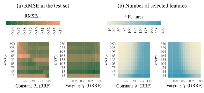
Figure 1: (a) Tiles plot for the average of resulting $\text{RMSE}_{\text{test}}$ and (b) number of selected features in a Regularized Random Forest and a Guided Regularized Random Forest varying mtry, $\lambda_{0}$ and $\gamma$. The number of selected features has a different relationship to mtry when comparing the two models. The $\text{RMSE}_{\text{{test}}}$ is generally lower for the GRRF, and the regularization gets very affected by mtry.

4.4 Generalized Regularization in Random Forests

For this subsection, we vary $\lambda_{0}=(0.1,0.5,0.9)$ and $\gamma=(0.001,0.25,0.5,0.75,0.99)$, use all combinations $(\gamma\times\lambda_{0})$, first with $g(\mathbf{x}_{i})=|corr(\mathbf{y},\mathbf{x}_{i})|$ and later using two Boosted methods, with a Standard Random Forest and with a Support Vector Machine. In Figure 2 we can see that $\text{RMSE}_{\text{test}}$ values are either close or below the 0.5 line. In comparison to Figure 1, our algorithms are doing better, as we can spot many cases where the $\text{RMSE}_{\text{test}}$ is low while using very few features, especially when $g(\mathbf{x}_{i})=\textit{Boosted}_{SVM}$. When $\gamma$ is low the regularization is primarily controlled by $\lambda_{0}$, and we spot a heavier influence of mtry on the number of selected features, which tends to decrease as $\lambda_{0}$ increases. When $\gamma$ is high the penalization values depend more on $g(\mathbf{x}_{i})$, and the results vary less regarding the values for $\lambda_{0}$ and mtry.

Table 2: Percentages of the most important and of correlated features selected and $\text{RMSE}_{\text{test}}$, averaged by mtry and $\gamma$. When using $g(\mathbf{x}_{i})=\text{Boosted}_{SVM}$, we pick more of the important features, less of the correlated and have lower $\text{RMSE}_{\text{test}}$. The results for the GRRF are shown for comparison.

	Correlation			$\text{Boosted}_{RF}$			$\text{Boosted}_{SVM}$
$\lambda_{0}$	% Imp.	% Corr.	$\text{RMSE}_{\text{test}}$	% Imp.	% Corr.	$\text{RMSE}_{\text{test}}$	% Imp.	% Corr.	$\text{RMSE}_{\text{test}}$
0.10	65.2%	18.8%	0.51	69%	33.2%	0.52	71%	21.6%	0.50
0.50	64.6%	19.0%	0.50	71.2%	28.2%	0.50	69.8%	20.8%	0.49
0.90	64.6%	20.0%	0.49	67.6%	22.4%	0.48	67.6%	22.4%	0.48

GRRF
$\gamma$	% Imp.	% Corr.	$\text{RMSE}_{\text{test}}$
$\approx$ 0.10	63.8%	33.1%	0.48
$\approx$ 0.50	67.6%	32.6%	0.48
$\approx$ 0.90	82.8%	32.0%	0.48

A more in-depth analysis of the results can be seen in Table 2. We define the most informative features in the simulation as $\mathcal{V}=(\mathbf{x_{1}},\mathbf{x_{2}},\mathbf{x_{3}},\mathbf{x_{4}},\mathbf{x_{5}},\underset{{i\in[6,205]\cap[0.9^{(i-5)/3}>0.01]}}{\mathbf{x_{i}}}).$ We do not include the last 45 features which are correlated and we ideally want to avoid them. We then calculate the percentage of important features from the total of features that were picked, and from the correlated ones, which percentage of those was selected by the algorithm. So, for example, if an algorithm picked 10 features, 3 of them being important, 5 being from the correlated group and 2 being "non-important", we calculate the proportion of important features as $3/5$ and the proportion of correlated as $5/45$. With Table 2 we see that the proportion of important features is considerably higher for our approach with $g(\mathbf{x}_{i})=\text{{Boosted}}_{RF}$ and $g(\mathbf{x}_{i})=\text{{Boosted}}_{SVM}$, and when we use $g(\mathbf{x}_{i})=|corr(\mathbf{y},\mathbf{x}_{i})|$ the algorithm picks less of the correlated variables. We also notice that the best results happened more or less when $\lambda_{0}\leq 0.5$, when $g(\mathbf{x}_{i})$ has a higher influence in the penalization coefficients, so they are really helping the feature selection. The GRRF algorithm usually picks more of the correlated features and, once, more of the important ones, but this model also picks more features in general.

Figure 2: $\text{RMSE}_{\text{test}}$ averages (with max-min intervals) and log number of features using the mixture of a $\lambda_{0}$ and a $g(\mathbf{x}_{i})$, for $g(\mathbf{x}_{i})=(|corr(\mathbf{y},\mathbf{x}_{i})|,\thinspace\text{Boosted}_{RF},\thinspace\text{Boosted}_{SVM}$). The x-axis shows the original scale, but the values are transformed to log. The models are use fewer features than the GRRF or Standard RF, with $\lambda_{0}$ and mtry visibly affecting the results.

4.5 Real Data Classification

Table 3: Average % of features used and average misclassification rates with standard deviation. The regularized models used far fewer features than a Standard RF. Clearly, our approaches uses far fewer features whilst maintaining competitive misclassification performance.

	Percentage of features used				Misclassification rate in the test set
Dataset	Std.RF	GRRF	$\text{Bst}_{RF}$	Mut.Inf.	Std.RF	GRRF	$\text{Bst}_{RF}$	Mut.Inf.
adenocarcinoma	9.38	0.83	0.86	0.07	3.45 (0.0)	11.03 (12)	3.4 (0.0)	10.77 (1.7)
brain	25.06	1.44	1.46	0.14	8.00 (5.6)	15.38 (14.4)	15.00 (7)	13.33 (10.5)
breast 2	24.44	1.76	1.79	0.14	25.6 (5.4)	20.7 (2)	17.8 (7.2)	20.7 (7.7)
breast 3	38.58	1.95	2.00	0.28	27.6 (6.4)	30.6 (4)	28.1 (3.8)	29.3 (1.6)
colon	34.44	2.53	2.60	0.44	4.76 (0.0)	5.71 (2.1)	6.67 (0.0)	7.78 (3)
leukemia	8.07	1.26	1.25	0.05	0.0 (0.0)	0.0 (0.0)	0.0 (0.0)	0.0 (0.0)
lymphoma	13.88	1.07	1.14	0.08	0.0 (0.0)	0.0 (0.0)	0.0 (0.0)	0.0 (0.0)
nci	44.77	1.81	1.88	0.16	30.77 (9.4)	38.95 (8)	37.5 (7.6)	43.75 (0.0)
prostate	18.22	1.46	1.40	0.09	0.54 (1.2)	0.54 (1.2)	1.08 (1.5)	0.54 (1.2)
srbct	29.69	2.26	2.25	0.3	0.0 (0.0)	0.0 (0.0)	0.91 (2)	1.74 (3.9)

Our experiments with real data consider gene classification micro-array datasets ([40], [37], [48], [3], [22], [2], [41], [44], [28]), with an average of 4787 features, 67 observations and 3 classes (details are in the Appendix A 1.1). Those are classical examples of "large p, small n" datasets, but our method generalizes to data from any contexts or sizes. As the goal here is to find the best features to predict the gene classes, the experiment conducted for this section is different. We run the regularized models and extract their selected features, that are later used in a Standard Random Forest, with which the misclassification rates are calculated. This is to mimic how such an approach can be used in practice, where first a discovery experiment is run to identify important features, then a subsequent algorithm is run on a new data set using all of the features. We set $\gamma=\lambda_{0}=0.5$, attributing the same weight to the baseline regularization and to $g(\mathbf{x}_{i})$. We vary $\texttt{mtry}=(\sqrt{p},0.15p,0.40p,0.75p,0.95p)$ and $g(\mathbf{x}_{i})=\Big{(}\text{Boosted}_{RF},\thinspace\frac{\text{MutInf}(\mathbf{y},\mathbf{x}_{i})}{max_{j=1}^{P}\text{MutInf}(\mathbf{y},\mathbf{x}_{j})}\Big{)}$. For comparison, we also run a Standard RF and a GRRF for each dataset, which were separated into 50 different train (2/3) and test sets (1/3). We first find the average misclassification rates (MR) and number of features used for each of the 50 resamples, eliminating at this step the mtry column. Out of that, we filter by the resample with the smallest MR. According to Table 5, the Standard RF uses more features, but does not always have the lowest MR. As for the regularization, using $g(\mathbf{x}_{i})=\Big{(}\frac{\text{MutInf}(\mathbf{y},\mathbf{x}_{i})}{max_{j=1}^{P}\text{MutInf}(\mathbf{y})}\Big{)}$ is better for [brain] and [prostate], while when $g(\mathbf{x}_{i})=\text{Boosted}_{RF}$, the results are good for the [adenocarcinoma], [breast 2], [breast 3] and [nci 60], and the GRRF is strictly better for the [colon] and [srbct] datasets, considering the MR. The MRs are all the same for the [leukemia] and [lymphona] datasets, but the percentage of features is often the lowest for our gain penalization method, especially when $g(\mathbf{x}_{i})=\Big{(}\frac{\text{MutInf}(\mathbf{y},\mathbf{x}_{i})}{max_{j=1}^{P}\text{MutInf}(\mathbf{y})}\Big{)}$. When this happens and such algorithms also have a low or very similar MR to a Standard RF one, we reach an optimal situation, which happened for almost all the datasets.

The comparison to LASSO [47] and varSelRF [18] is presented in the Appendix A 1.2 (only 10 resamples were done for these models due to their computational heaviness).

5 Implementation

The implementation is included as an extension to the ranger package [49], which is originally written in C++ and is currently the fastest tree model implementation available for R [rmanual]. Furthermore, the package has a wide variety of model extensions, is actively maintained and interfaces with python. The speed and scalability discussion presented in Wright & Ziegler [49] and its comparison to the randomForest package [29] is analogous to the one about our regularization implemented in the ranger and the one in the RRF package, so we do not repeat the same experiments.

6 Conclusions and next steps

Feature selection and regularization for tree-based methods is a topic of active research. In this work, we have demonstrated that our gain penalization generalization, which combines previous information about the features with a baseline penalization $\lambda_{0}$, produces good results in terms of the (number of features) x (prediction error) trade-off. Along with the methodology, we make the implementation available in the fastest Random Forest package for R.

The downside of our approach is the addition of new hyperparameters, and how to choose them well. Future work involves finding theoretical properties of certain gain penalization approaches, parameter optimization (using e.g. Snoek et al. [45]), and compare our approach to other methods with a similar context (Johnson & Zhang [27], Nan & Saligrama [32], Nan et al. [33], for example).

Appendix A Appendix

A.1 Dataset descriptions

Table 4: Datasets’ specifications. Problematic $p>n$ situation in all cases.

Dataset	Ref.	Obs.	Features	Classes
adenocarcinoma	[40]	76	9869	2
brain	[37]	42	5598	5
breast 2	[48]	77	4870	2
breast 3	[48]	95	4870	3
colon	[3]	62	2001	2
leukemia	[22]	38	3052	2
lymphoma	[2]	62	4027	3
nci 60	[41]	61	5245	8
prostate	[44]	102	6034	2
srbct	[28]	63	2309	4

A.2 LASSO and varSelRF results

In Table 5, we present the classification results added with the LASSO and varSelRF results. Only 10 resamples were done for these algorithms due to their computational heaviness. We can see that the LASSO and varSelRF can select very few variables but at the expense of the prediction error. Their variable selection results are more closely comparable to our regularized model using $g(\mathbf{x}_{i})=\Big{(}\frac{\text{MutInf}(\mathbf{y},\mathbf{x}_{i})}{max_{j=1}^{P}\text{MutInf}(\mathbf{y})}\Big{)}$, but their prediction error is much higher.

Table 5: Average % of features used and average misclassification rates with standard deviation added with the LASSO and varSelRF results. The regularized models used far fewer features than a Standard RF. Clearly, our approaches use far fewer features whilst maintaining competitive misclassification performance.

	Percentage of features used
Dataset	Std.RF	GRRF	$\text{Bst}_{RF}$	Mut.Inf.	LASSO	varSelRF
adenocarcinoma	9.38	0.83	0.86	0.07	0.02	0.05
brain	25.06	1.44	1.46	0.14	0.39	0.73
breast 2	24.44	1.76	1.79	0.14	0.21	0.34
breast 3	38.58	1.95	2.00	0.28	0.67	0.28
colon	34.44	2.53	2.60	0.44	0.46	0.94
leukemia	8.07	1.26	1.25	0.05	0.28	0.09
lymphoma	13.88	1.07	1.14	0.08	0.34	0.72
nci	44.77	1.81	1.88	0.16	1.11	0.97
prostate	18.22	1.46	1.40	0.09	0.14	0.07
srbct	29.69	2.26	2.25	0.3	0.68	0.99

	Misclassification rate in the test set
Dataset	Std.RF	GRRF	$\text{Bst}_{RF}$	Mut.Inf.	LASSO	varSelRF
adenocarcinoma	3.45 (0.0)	11.03 (12)	3.4 (0.0)	10.77 (1.7)	13.83 (6.4)	19.6 (7.7)
brain	8.00 (5.6)	15.38 (14.4)	15.00 (7)	13.33 (10.5)	27.6 (11.7)	29 (16.2)
breast 2	25.6 (5.4)	20.7 (2)	17.8 (7.2)	20.7 (7.7)	31.56 (5.19)	36.7 (9.1)
breast 3	27.6 (6.4)	30.6 (4)	28.1 (3.8)	29.3 (1.6)	29.7 (4.85)	33.9 (8.6)
colon	4.76 (0.0)	5.71 (2.1)	6.67 (0.0)	7.78 (3)	16.7 (8.6)	23.06 (8.3)
leukemia	0.0 (0.0)	0.0 (0.0)	0.0 (0.0)	0.0 (0.0)	10.07 (9.4)	13.2 (12)
lymphoma	0.0 (0.0)	0.0 (0.0)	0.0 (0.0)	0.0 (0.0)	1.48 (4.7)	5.86 (4.8)
nci	30.77 (9.4)	38.95 (8)	37.5 (7.6)	43.75 (0.0)	42.2 (7.5)	44.7 (12.8)
prostate	0.54 (1.2)	0.54 (1.2)	1.08 (1.5)	0.54 (1.2)	6 (2.8)	8.87 (1.9)
srbct	0.0 (0.0)	0.0 (0.0)	0.91 (2)	1.74 (3.9)	1.33 (2.9)	4.5 (3.6)

References

- Ler [1977] Toward a Formal Theory of Tonal Music. Journal of Music Theory, 1977. ISSN 00222909. doi: 10.2307/843480.
- Alizadeh et al. [2000] Alizadeh, A. A., Eisen, M. B., Davis, R. E., Ma, C., Lossos, I. S., Rosenwald, A., Boldrick, J. C., Sabet, H., Tran, T., Yu, X., et al. Distinct types of diffuse large b-cell lymphoma identified by gene expression profiling. Nature, 403(6769):503, 2000.
- Alon et al. [1999] Alon, U., Barkai, N., Notterman, D. A., Gish, K., Ybarra, S., Mack, D., and Levine, A. J. Broad patterns of gene expression revealed by clustering analysis of tumor and normal colon tissues probed by oligonucleotide arrays. Proceedings of the National Academy of Sciences, 96(12):6745–6750, 1999.
- Athey et al. [2016] Athey, S., Tibshirani, J., and Wager, S. Generalized Random Forests. oct 2016. URL https://arxiv.org/abs/1610.01271.
- Breiman [1996] Breiman, L. Bagging predictors. Machine Learning, 24(2):123–140, Aug 1996. ISSN 1573-0565. doi: 10.1023/A:1018054314350. URL https://doi.org/10.1023/A:1018054314350.
- Breiman [2001] Breiman, L. Random Forests. Machine Learning, 2001. ISSN 1098-6596. doi: 10.1017/CBO9781107415324.004.
- Breiman [2017] Breiman, L. Classification and regression trees. Routledge, 2017.
- Breiman et al. [1984] Breiman, L., Friedman, J., Stone, C., and Olshen, R. Classification and Regression Trees. The Wadsworth and Brooks-Cole statistics-probability series. Taylor & Francis, 1984. ISBN 9780412048418. URL https://books.google.ie/books?id=JwQx-WOmSyQC.
- Chen & Popovich [2002] Chen, P. and Popovich, P. Correlation: parametric and nonparametric measures. Number Nº 137-139 in Sage university papers series. no. 07-139. Sage Publications, 2002. ISBN 9780761922285. URL https://books.google.ie/books?id=UN4nAQAAIAAJ.
- Chipman et al. [2010] Chipman, H. A., George, E. I., and McCulloch, R. E. BART: Bayesian additive regression trees. Annals of Applied Statistics, 2010. ISSN 19326157. doi: 10.1214/09-AOAS285.
- Cohen [1960] Cohen, J. A Coefficient of Agreement for Nominal Scales. Educational and Psychological Measurement, 1960. ISSN 15523888. doi: 10.1177/001316446002000104.
- Cortez [2016] Cortez, P. rminer: Data Mining Classification and Regression Methods, 2016. URL https://CRAN.R-project.org/package=rminer. R package version 1.4.2.
- Cortez & Embrechts [2013] Cortez, P. and Embrechts, M. J. Using sensitivity analysis and visualization techniques to open black box data mining models. Information Sciences, 225:1 – 17, 2013. ISSN 0020-0255. doi: https://doi.org/10.1016/j.ins.2012.10.039. URL http://www.sciencedirect.com/science/article/pii/S0020025512007098.
- Deng [2013] Deng, H. Guided random forest in the rrf package. arXiv preprint arXiv:1306.0237, 2013.
- Deng & Runger [2012a] Deng, H. and Runger, G. Feature selection via regularized trees. In The 2012 International Joint Conference on Neural Networks (IJCNN), pp. 1–8. IEEE, 2012a.
- Deng & Runger [2013] Deng, H. and Runger, G. Gene selection with guided regularized random forest. Pattern Recognition, 46(12):3483–3489, 2013.
- Deng & Runger [2012b] Deng, H. and Runger, G. C. Gene selection with guided regularized random forest. CoRR, abs/1209.6425, 2012b. URL http://arxiv.org/abs/1209.6425.
- Diaz-Uriarte [2007] Diaz-Uriarte, R. GeneSrF and varSelRF: a web-based tool and R package for gene selection and classification using random forest. 2007. doi: 10.1186/1471-2105-8-328. URL http://www.biomedcentral.com/1471-2105/8/328.
- Díaz-Uriarte & Alvarez de Andrés [2006] Díaz-Uriarte, R. and Alvarez de Andrés, S. Gene selection and classification of microarray data using random forest. BMC Bioinformatics, 2006. ISSN 14712105. doi: 10.1186/1471-2105-7-3.
- Friedman & Popescu [2008] Friedman, J. and Popescu, B. Predictive learning via rule ensembles. The Annals of Applied Statistics, 2, 12 2008. doi: 10.1214/07-AOAS148.
- Friedman [1991] Friedman, J. H. Rejoinder: Multivariate Adaptive Regression Splines. The Annals of Statistics, 1991. ISSN 0090-5364. doi: 10.1214/aos/1176347973.
- Golub et al. [1999] Golub, T. R., Slonim, D. K., Tamayo, P., Huard, C., Gaasenbeek, M., Mesirov, J. P., Coller, H., Loh, M. L., Downing, J. R., Caligiuri, M. A., et al. Molecular classification of cancer: class discovery and class prediction by gene expression monitoring. science, 286(5439):531–537, 1999.
- Guyon & Elisseeff [2003] Guyon, I. and Elisseeff, A. An introduction to variable and feature selection. J. Mach. Learn. Res., 3:1157–1182, March 2003. ISSN 1532-4435. URL http://dl.acm.org/citation.cfm?id=944919.944968.
- Hastie et al. [2009] Hastie, T., Tibshirani, R., and Friedman, J. The Elements of Statistical Learning. Elements, 1:337–387, 2009. ISSN 03436993. doi: 10.1007/b94608. URL http://www.springerlink.com/index/10.1007/b94608.
- Hastie, Trevor, Tibshirani, Robert, Friedman [2009] Hastie, Trevor, Tibshirani, Robert, Friedman, J. The Elements of Statistical Learning, Second Edition. 2009. ISBN 978-0-387-84858-7. doi: 10.1007/978-0-387-84858-7.
- Hoerl & Kennard [1970] Hoerl, A. E. and Kennard, R. W. Ridge Regression: Biased Estimation for Nonorthogonal Problems. Technometrics, 1970. ISSN 15372723. doi: 10.1080/00401706.1970.10488634.
- Johnson & Zhang [2013] Johnson, R. and Zhang, T. Learning nonlinear functions using regularized greedy forest. IEEE transactions on pattern analysis and machine intelligence, 36(5):942–954, 2013.
- Khan et al. [2001] Khan, J., Wei, J. S., Ringner, M., Saal, L. H., Ladanyi, M., Westermann, F., Berthold, F., Schwab, M., Antonescu, C. R., Peterson, C., et al. Classification and diagnostic prediction of cancers using gene expression profiling and artificial neural networks. Nature medicine, 7(6):673, 2001.
- Liaw & Wiener [2002] Liaw, A. and Wiener, M. Classification and regression by randomforest. R News, 2(3):18–22, 2002. URL https://CRAN.R-project.org/doc/Rnews/.
- Louppe [2014] Louppe, G. Understanding Random Forests: From Theory to Practice. PhD thesis, 10 2014.
- Murphy [2012] Murphy, K. P. Machine learning - a probabilistic perspective. In Adaptive computation and machine learning series, 2012.
- Nan & Saligrama [2017] Nan, F. and Saligrama, V. Adaptive classification for prediction under a budget. In Advances in Neural Information Processing Systems, pp. 4727–4737, 2017.
- Nan et al. [2016] Nan, F., Wang, J., and Saligrama, V. Pruning random forests for prediction on a budget. In Advances in neural information processing systems, pp. 2334–2342, 2016.
- Nascimento & Coelho [2009] Nascimento, D. S. and Coelho, A. L. Ensembling heterogeneous learning models with boosting. In International Conference on Neural Information Processing, pp. 512–519. Springer, 2009.
- Nelder & Wedderburn [1972] Nelder, J. A. and Wedderburn, R. W. Generalized linear models. Journal of the Royal Statistical Society: Series A (General), 135(3):370–384, 1972.
- Pérez-Sancho et al. [2010] Pérez-Sancho, C., Rizo, D., Iesta, J. M., De León, P. J., Kersten, S., and Ramirez, R. Genre classification of music by tonal harmony. Intelligent Data Analysis, 2010. ISSN 1088467X. doi: 10.3233/IDA-2010-0437.
- Pomeroy et al. [2002] Pomeroy, S. L., Tamayo, P., Gaasenbeek, M., Sturla, L. M., Angelo, M., McLaughlin, M. E., Kim, J. Y., Goumnerova, L. C., Black, P. M., Lau, C., et al. Prediction of central nervous system embryonal tumour outcome based on gene expression. Nature, 415(6870):436, 2002.
- Quinlan [1986] Quinlan, J. R. Induction of decision trees. Machine Learning, 1:81–106, 1986.
- R Core Team [2018] R Core Team. R: A Language and Environment for Statistical Computing. R Foundation for Statistical Computing, Vienna, Austria, 2018. URL https://www.R-project.org/.
- Ramaswamy et al. [2003] Ramaswamy, S., Ross, K. N., Lander, E. S., and Golub, T. R. A molecular signature of metastasis in primary solid tumors. Nature genetics, 33(1):49–54, 2003.
- Ross et al. [2000] Ross, D. T., Scherf, U., Eisen, M. B., Perou, C. M., Rees, C., Spellman, P., Iyer, V., Jeffrey, S. S., Van de Rijn, M., Waltham, M., et al. Systematic variation in gene expression patterns in human cancer cell lines. Nature genetics, 24(3):227, 2000.
- SHANNON [1948] SHANNON, C. A mathematical theory of communication. 1948.
- Shannon [1948] Shannon, C. E. A mathematical theory of communication. Bell system technical journal, 27(3):379–423, 1948.
- Singh et al. [2002] Singh, D., Febbo, P. G., Ross, K., Jackson, D. G., Manola, J., Ladd, C., Tamayo, P., Renshaw, A. A., D’Amico, A. V., Richie, J. P., et al. Gene expression correlates of clinical prostate cancer behavior. Cancer cell, 1(2):203–209, 2002.
- Snoek et al. [2012] Snoek, J., Larochelle, H., and Adams, R. P. Practical bayesian optimization of machine learning algorithms. In Proceedings of the 25th International Conference on Neural Information Processing Systems - Volume 2, NIPS’12, pp. 2951–2959, USA, 2012. Curran Associates Inc. URL http://dl.acm.org/citation.cfm?id=2999325.2999464.
- Strobl et al. [2008] Strobl, C., Boulesteix, A.-L., Kneib, T., Augustin, T., and Zeileis, A. Conditional variable importance for random forests. BMC bioinformatics, 9:307, 08 2008. doi: 10.1186/1471-2105-9-307.
- Tibshirani [1991] Tibshirani, R. Regression shrinkage and selection via the Lasso. Journal of the Royal Statistical Society. Series B (Methodological), 1991. ISSN 0035-9246. doi: 10.2307/2346101.
- Van’t Veer et al. [2002] Van’t Veer, L. J., Dai, H., Van De Vijver, M. J., He, Y. D., Hart, A. A., Mao, M., Peterse, H. L., Van Der Kooy, K., Marton, M. J., Witteveen, A. T., et al. Gene expression profiling predicts clinical outcome of breast cancer. nature, 415(6871):530, 2002.
- Wright & Ziegler [2017] Wright, M. N. and Ziegler, A. ranger: A fast implementation of random forests for high dimensional data in C++ and R. Journal of Statistical Software, 77(1):1–17, 2017. doi: 10.18637/jss.v077.i01.