Bayesian Group Learning for Shot Selection of Professional Basketball Players

Abstract

In this paper, we develop a group learning approach to analyze the underlying heterogeneity structure of shot selection among professional basketball players in the NBA. We propose a mixture of finite mixtures (MFM) model to capture the heterogeneity of shot selection among different players based on Log Gaussian Cox process (LGCP). Our proposed method can simultaneously estimate the number of groups and group configurations. An efficient Markov Chain Monte Carlo (MCMC) algorithm is developed for our proposed model. Simulation studies have been conducted to demonstrate its performance. Ultimately, our proposed learning approach is further illustrated in analyzing shot charts of selected players in the NBA’s 2017–2018 regular season.

Keywords: Basketball Shot Charts; Heterogeneity Pursuit; Log Gaussian Cox Process; Mixture of Finite Mixtures; Nonparameteric Bayesian

1 Introduction

In basketball data analytics, one primary problem of research interest is to study how players choose the locations to make shots. Shot charts, which are graphical representations of players’ shot location selections, provide important summary of information for basketball coaches as well as teams’ data analysts, as no good defense strategies can be made without understanding the shot selection habits of players in the rival teams. Shot selection data have been discussed from different statistical perspectives. Reich et al. (2006) developed a spatially varying coefficients model for shot-chart data, where the court is divided into small regions, and the probability of making a shot in these zones are modeled using the multinomial logit approach. Recognizing the random nature of shot location selection, Miller et al. (2014) analyzed the underlying spatial structure among professional basketball players based on spatial point processes. Franks et al. (2015) combined spatial and spatio-temporal processes, matrix factorization techniques and hierarchical regression models for characterizing the spatial structure of locations for shot attempts. In spatial point processes, locations for points are assumed random, and are regarded as realizations of a process governed by an underlying intensity. Spatial point processes are well discussed in many statistical literatures, such as the Poisson process (Geyer, 1998), the Gibbs process (Goulard et al., 1996), and the Log Gaussian Cox process (LGCP; Møller et al., 1998). In addition, they have been applied to different areas, such as ecological studies (Thurman et al., 2015; Jiao et al., 2020), environmental sciences (Veen and Schoenberg, 2006; Hu et al., 2019), and sports analytics (Miller et al., 2014; Jiao et al., 2019). Most existing literatures concentrate on parametric (Guan, 2008) or nonparametric (Guan, 2008; Geng et al., 2019) estimation of the underlying intensities for spatial point process and analysis of second-order properties (Diggle et al., 2007). There are very limited literatures discussing the grouping pattern of multiple point processes. Knowing the group information of different point processes will lead to discovery of the underlying heterogeneity structure of different players.

Jiao et al. (2019) proposed a joint model approach for basketball shot chart data. After model parameter estimates are obtained for different players, they are grouped via ad hoc clustering approaches, such as hierarchical clustering. Chen et al. (2019) developed a group linked Cox process model for analyzing point of interest (POI) data in Beijing. To determine the number of groups, starting from the most complicated model where each observation has its own group, a loss function is used in a series of hierarchical merging steps to combine the groups. In both methods, the inherent uncertainty in estimation for the number of groups is ignored. In contrast, Bayesian models such as the Dirichlet process (DP; Ferguson, 1973) offer a natural solution that simultaneously estimates the number of groups and group configurations. However, Miller and Harrison (2013) shows that Dirichlet process mixture model (DPMM) tends to create tiny extraneous groups. In other words, DPMM does not produce consistent estimator of the number of groups. In this paper, we employ the mixture of finite mixture (MFM; Miller and Harrison, 2018) approach for learning the group structure of multiple spatial point processes, which, on the contrary, provides consistent estimation for group numbers.

The contribution of this paper is two-fold. First, we propose a Bayesian group learning method to simultaneously estimate the number of groups and the group configurations. In particular, we use an LGCP to model the spatial pattern of the shot attempts. Based on similarity matrices of fitted intensity among different players, a MFM model is incorporated for group learning. Moreover, the MFM model has a Pólya urn scheme similar to the Chinese restaurant process, which is exploited to develop an efficient Markov chain Monte Carlo MCMC algorithm without reversible jump or even allocation samplers. Compared with existing approaches (e.g., Jiao et al., 2019), our proposed method does not require prior information for the number of groups, and grouping is incorporated into the structure of the model and performed directly based on shot selection intensity instead of via ad hoc analysis of regression coefficients. In addition, our proposed Bayesian approach reveals interesting shooting patterns of professional basketball players, and the summaries better characterize player types beyond the traditional position categorization.

The rest of the paper is organized as follows. In Section 2, the shot chart data of different players from the 2017–2018 NBA regular season is introduced. In Section 3, we discuss the LGCP and develop the Bayesian group learning method based on MFM. Details of the Bayesian inference are presented in Section 4, including the MCMC algorithm and post MCMC inference methods. Simulation studies are conducted in Section 5. Applications of the proposed methods to NBA players data are reported in Section 6. Section 7 concludes the paper with a discussion.

2 Motivating Data

Our data consists of both made and missed field goal attempt locations from the offensive half court of games in the 2017–2018 National Basketball Association (NBA) regular season. The data is available at http://nbasavant.com/index.php. We focus on players that have made more than 400 field goal attempts (FTA). Also, players who just started their careers in the 2017–2018 season, such as Lonzo Ball and Jayson Tatum, are not considered. A total of 191 plays who meet the two criteria above are included in our analysis.

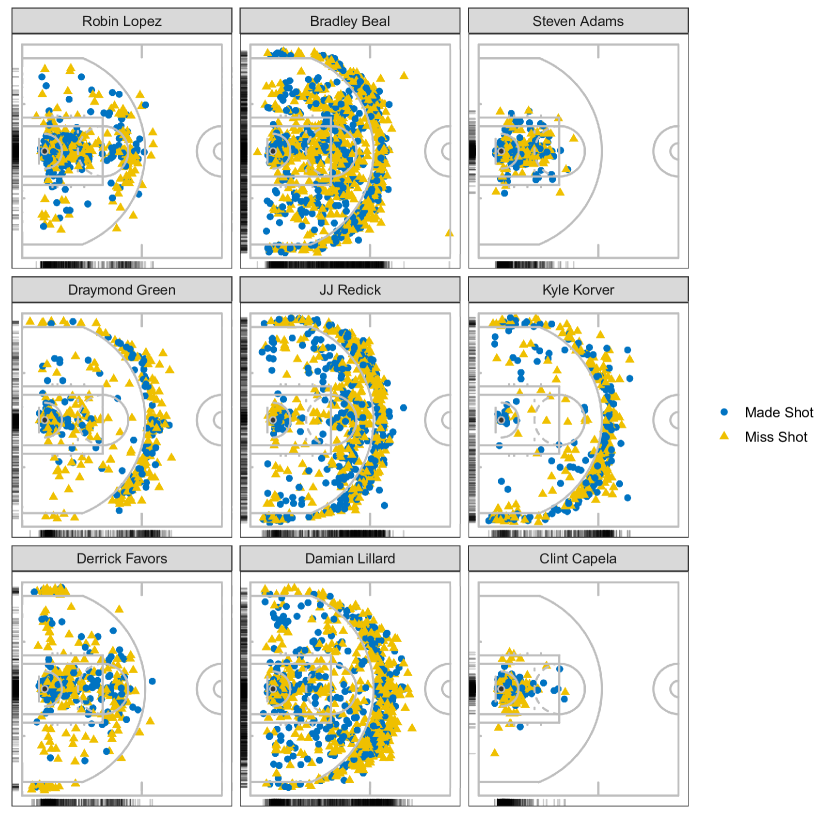
Figure 1: Shot charts for selected NBA players.

We model a player’s shooting location choices as a spatial point pattern on the offensive half court, a 47 ft by 50 ft rectangle, which is the standard size for NBA. We assume the spatial domain $D\in[0,47]\times[0,50]$. Indexing the players with $i\in\{1,\ldots,191\}$, the locations of shots, both made and missed, for player $i$ are denoted as $X_{i}=\{x_{i,1},\ldots,x_{i,T_{i}}\}$, $\forall x_{i,T_{i}}\in D$, where $T_{i}$ is the total number of attempts made by player $i$ on the offensive half court. We select nine players and visualize their shot charts in Figure 1. It can be seen that Clint Capela makes more shot attempts in the painted area, as most of his field goals are slam dunks. JJ Redick, however, prefers to shoot outside the painted area. Our goal is to find groups of similar shooting location habits among the NBA basketball players.

3 Method

3.1 Log-Gaussian Cox Process

The shot locations can be denoted as $y=(\bm{s}_{1},\ldots,\bm{s}_{\ell})$, with $(\bm{s}_{1},\ldots,\bm{s}_{\ell})$ being the locations of points that are observed within a bounded region $\mathcal{B}\subseteq\mathcal{R}^{2}$. Such spatial point pattern can be regarded as a realization from a spatial point process $Y$. Spatial point pattern data are modeled by spatial point processes (Diggle et al., 1976) characterized by a quantity called intensity. Within a region $\mathcal{B}$, the intensity on any location $\bm{s}\in\mathcal{B}$ can be represented as $\lambda(\bm{s})$, which is defined as:

$$\lambda(\bm{s})=\lim_{|\differential\bm{s}\rightarrow 0|}\left(\frac{\textrm{E}[N(\differential\bm{s})]}{|\differential\bm{s}|}\right),$$

where $\differential\bm{s}$ is an infinitesimal region around $\bm{s}$, $|\differential\bm{s}|$ represents its area, and $N(\differential\bm{s})$ shows the number of events that happened over $\differential\bm{s}$. For an area $A\subseteq\mathcal{B}$, we denote by $N_{\bm{Y}}(A)=\sum_{i=1}^{\ell}1(s_{i}\in A)$ the counting process associated with the spatial point process $\bm{Y}$, which counts the number of points in a realization of $\bm{Y}$ that fall within an area $A\subseteq\mathcal{B}$. The Poisson distribution has been conventionally used for modeling count data, and correspondingly, the spatial Poisson point process is a popular tool for modeling spatial point pattern data. For a Poisson process $Y$ over $\mathcal{B}$, with its intensity function denoted as $\lambda(\bm{s})$, the counting process $N_{Y}(A)$ satisfies:

$$N_{Y}(A)\sim\mbox{Poisson}(\lambda(A)),\mbox{ where }\lambda(A)=\int_{A}\lambda(\bm{s})\differential\bm{s}.$$

For the Poisson process, it is easy to obtain $E(N_{\bm{Y}}(A))=\text{Var}(N_{\bm{Y}}(A))=\lambda(A)$. When $\lambda(\bm{s})=\lambda$, we have constant intensity over the space $\mathcal{B}$ and in this special case, $\bm{Y}$ reduces to a homogeneous Poisson process (HPP). For a more general case, $\lambda(\bm{s})$ can be spatially varying, which leads to a nonhomogeneous Poisson process (NHPP). For the NHPP, the log-likelihood on $\mathcal{B}$ for the observed dataset $\bm{y}$ is given by

$$\ell=\sum_{i=1}^{k}\text{log}\lambda(s_{i})-\int_{\mathcal{B}}\lambda(s)\differential s,$$ (1)

where $\lambda(s_{i})$ is the intensity function for location $s_{i}$. We signify that a set of points $\bm{y}=(s_{1},s_{2},...,s_{\ell})$ follows a Poisson process as

$$\bm{y}\sim\mathcal{PP}(\lambda(\cdot)).$$ (2)

A log-Gaussian Cox process (LGCP) is a doubly-stochastic Poisson process with a spatially varying intensity function modeled as an exponentiated Gaussian process, i.e., Gaussian random field (GRF; Rasmussen and Williams, 2006), which is a spatially continuous random process in which random variables at any location in a space are normally distributed, and are correlated with random variables at other locations according to a continuous correlation process. The LGCP can be written hierarchically as

$$\begin{split}\bm{y}&\sim\mathcal{PP}(\lambda(\cdot)),\\ \lambda(\cdot)&=\exp(Z(\cdot)),\\ Z(\cdot)&\sim\mathcal{GP}(0,k(\cdot,\cdot)),\end{split}$$ (3)

where $k(\cdot,\cdot)$ is the covariance function of the Gaussian process, $Z(\cdot)$. For estimation, the GRF is approximated by the solution to a stochastic partial differential equation (SPDE; see, Lindgren et al., 2011, for a review), as SPDEs provide an efficient way of approximating the GRF in continuous space (Simpson et al., 2016). Under a purely Bayesian paradigm, model-based Markov chain Monte Carlo (MCMC) can be time-consuming for LGCP. Therefore, we compute the LGCP using the integrated nested Laplace approximation (INLA; Rue et al., 2009), which is an alternative to MCMC for fitting latent Gaussian models that provides a fast and accurate way to fit a potential model, and facilitates computationally efficient inference on point processes. For more details about INLA, we refer the reader to the R-INLA project website at http://www.r-inla.org. Details about computation is directed to Section 4.

With estimated intensity surfaces for $n$ different players, denoted as $\widehat{\lambda}^{(1)}(\cdot),\ldots,\widehat{\lambda}^{(n)}(\cdot)$. With our main goal being to group players who share similar shot location choices over the court, an appropriate metric is needed to quantify similarities among the intensities. Let the matrix C be that $\textbf{C}\equiv(\widehat{\lambda}^{(1)},\widehat{\lambda}^{(2)},\ldots,\widehat{\lambda}^{(n)})$, and denote $\textbf{C}^{(i)}=\lambda^{(i)}$. Then, following the approach in Cervone et al. (2016), we compute the players’ similarity matrix H as:

$$\text{H}_{i,j}=\exp\left\{-\left\|\frac{\textbf{C}^{(i)}}{\sum\textbf{C}^{(i)}}-\frac{\textbf{C}^{(j)}}{\sum\textbf{C}^{(j)}}\right\|\right\},$$ (4)

where $i,j\in\{1,\ldots,n\}$ and $\left\|\cdot\right\|$ is $L_{2}$ norm. It can be seen that H is symmetric, and $\textbf{H}\in\mathcal{R}^{n\times n}$.

3.2 Group Learning via Point Process Intensity

With the similarity matrix H obtained, we employ nonparametric Bayesian methods to detect grouped patterns in the intensities. Our initial step is to transform the similarity matrix H so that each entry $H_{i,j}$ is within the range of a Gaussian distribution. Denote the fisher transformed distance matrix (fisher1915frequency) as $\bm{\mathscr{\bm{S}}}$. Its $(i,j)$th element is calculated as

$$\mathscr{S}_{ij}=\frac{1}{2}\log\left(\dfrac{1+\text{H}_{i,j}}{1-\text{H}_{i,j}}\right),$$ (5)

A larger value of $\mathscr{S}_{ij}$ indicate higher similarity of intensities. We further assume that

$$\begin{split}\mathscr{S}_{ij}&\mid\bm{\mu},\bm{\tau},k\sim\mbox{N}(\mu_{ij},\tau_{ij}^{-1}),\quad\mu_{ij}=U_{z_{i}z_{j}}\\ \tau_{ij}&=T_{z_{i}z_{j}},\quad 1\leq i<j\leq n,\end{split}$$ (6)

where $k$ denotes the number of groups, $\mbox{N}()$ denotes the normal distribution, $z_{i}\in\{1,\ldots,k\}$ denotes the group membership of player $i$ for $i=1,\ldots,191$. The matrices $\bm{U}=[U_{rs}]\in(-\infty,+\infty)^{k\times k}$ and $\bm{T}=[T_{rs}]\in(0,+\infty)^{k\times k}$ are both symmetric, with $U_{rs}=U_{sr}$ indicating the mean closeness between any two fitted intensity surfaces in groups $r$ and $s$, respectively, and $T_{rs}=T_{sr}$ indicating the precision.

Denote by $\mathcal{Z}_{n,k}=\big{\{}(z_{1},\ldots,z_{n}):z_{i}\in\{1,\ldots,k\},1\leq i\leq n\big{\}}$ the set of all possible partitions of $n$ players into $k$ groups. With certain $z\in\mathcal{Z}_{n,k}$, denote by $\mathscr{S}_{[rs]}$ the $n_{r}\times n_{s}$ sub-matrix of $\mathscr{S}$ consisting of entries $\mathscr{S}_{ij}$ where $z_{i}=r$ and $z_{j}=s$. Under model (6), the joint likelihood of $\mathscr{S}$ can be written as

$$\begin{split}P(\bm{\mathscr{S}}\mid\bm{z},\bm{U},\bm{T},k)=\prod_{1\leq r\leq s\leq k}P(\bm{\mathscr{S}}_{[rs]}\mid\bm{z},\bm{U},\bm{T}),\end{split}$$ (7)

where

$$\begin{split}P(\bm{\mathscr{S}}_{[rs]}\mid\bm{z},\bm{U},\bm{T})=\prod_{1\leq i<j\leq n:z_{i}=r,z_{j}=s}\frac{1}{\sqrt{2\pi T_{rs}^{-1}}}\exp\left\{-\frac{T_{rs}(\mathscr{S}_{ij}-U_{rs})^{2}}{2}\right\}.\end{split}$$

Assuming that the number of groups $k$ is given, independent prior distributions are often assigned to $z$, $U$, and $T$. Such specification can be conveniently incorporated into a finite mixture model. When $k$ is unknown, however, the Dirichlet process mixture prior models (Antoniak, 1974) can be employe as:

$$\bm{\mathscr{S}}_{i}\sim F(.,\bm{\theta}_{i}),\quad\bm{\theta}_{i}\sim G(.),\quad G\sim DP(\alpha G_{0}),$$ (8)

with $\bm{\mathscr{S}_{i}}=(\mathscr{S}_{i1},\mathscr{S}_{i2},\ldots,\mathscr{S}_{in})$, $\bm{\theta}_{i}=(\bm{\theta}_{i1},\bm{\theta}_{i2},\ldots,\bm{\theta}_{in})$ and $\bm{\theta}_{ij}=(\mu_{ij},\tau_{ij})$. The process $G$ is parameterized by a base measure $G_{0}$ and a concentration parameter $\alpha$. With $\bm{\theta}_{i}$ for $i=1,\ldots,n$ drawn from $G$, a conditional prior distribution for a newly drawn $\bm{\theta}_{n+1}$ can be obtained via integration (Blackwell et al., 1973):

$$p(\bm{\theta}_{n+1}\mid\bm{\theta}_{1},\ldots,\bm{\theta}_{n})=\dfrac{1}{n+\alpha}\sum_{i=1}^{n}\delta_{\bm{\theta}_{i}}(\bm{\theta}_{n+1})+\dfrac{\alpha}{n+\alpha}G_{0}(\bm{\theta}_{n+1}),$$ (9)

with $\delta_{\bm{\theta}_{i}}(\bm{\theta}_{j})=I(\bm{\theta}_{j}=\bm{\theta}_{i})$ being the point mass at $\bm{\theta}_{i}$. The model can be equivalently obtained with the introduction of group membership $z_{i}$’s and having $K$, the number of groups, approach infinity (Neal, 2000):

$$\begin{split}\bm{\mathscr{S}}_{i}\mid z_{i},\bm{\theta}^{*}&\sim F(\bm{\theta}^{*}_{z_{i}}),\\ z_{i}\mid\bm{\pi}&\sim\text{Discrete}(\pi_{1},\ldots,\pi_{K}),\\ \bm{\theta}^{*}_{c}&\sim G_{0},\\ \bm{\pi}&\sim\text{Dirichlet}(\alpha/K,\ldots,\alpha/K),\end{split}$$ (10)

where $\bm{\pi}=(\pi_{1},\ldots,\pi_{K})$. It can be seen that under this construction, the group-specific distribution $F(\cdot\mid\bm{\theta}_{c}^{*})$ solely depends on the vector of parameters $\bm{\theta}^{*}_{c}$.

In construction (10), the prior distribution of $(z_{1},\ldots,z_{n})$, which would allow for automatic inference on the number of groups $k$, can be obtained by integrating out $\bm{\pi}$, the mixing proportions. This is also known as the Chinese restaurant process (CRP; Aldous, 1985; Pitman, 1995; Neal, 2000). The conditional distribution for $z_{i}$ is defined through the metaphor of a Chinese restaurant (Blackwell et al., 1973):

$$P(z_{i}=c\mid z_{1},\ldots,z_{i-1})\propto\begin{cases}|c|,&\text{at an existing table labeled}\,c\\ \alpha,&\text{if}\,$c$\,\text{is a new table}\end{cases},$$ (11)

where $|c|$ denotes the size of group $c$. Despite its ability to simultaneously estimate the number of groups and group configuration, the CRP has been shown by Miller and Harrison (2018) to produce redundant tail groups, causing inconsistency in estimation for the number of groups even with the sample size going to infinity. Miller and Harrison (2018) also proposed a modification of the CRP, known as the mixture of finite mixtures (MFM) model, to mitigate this problem. The MFM model can be formulated as:

$$k\sim p(\cdot),\quad(\pi_{1},\ldots,\pi_{k})\mid k\sim\mbox{Dirichlet}(\gamma,\ldots,\gamma),\quad z_{i}\mid k,\bm{\pi}\sim\sum_{h=1}^{k}\pi_{h}\delta_{h},\quad i=1,\ldots,n,$$ (12)

with $p(\cdot)$ being a proper probability mass function on the set of positive integers, and $\delta_{h}$ being a point mass at $h$. Define a coefficient $V_{n}(w)$ as

$$V_{n}(w)=\sum_{k=1}^{+\infty}\dfrac{k_{(w)}}{(\gamma k)^{(n)}}p(k),$$

where $w$ denotes the number of “existing tables”, $k_{(w)}=k(k-1)\ldots(k-w+1)$, and $(\gamma k)^{(n)}={\gamma k}(\gamma k+1)\ldots(\gamma k+n-1)$, $x^{(0)}=1$, and $x_{(0)}=1$. Introduction of a new table is slowed down by $V_{n}(w+1)/V_{n}(w)$, which yields the following conditional prior of $\bm{\theta}$:

$$P(\bm{\theta}_{n+1}\mid\bm{\theta}_{1},\ldots,\bm{\theta}_{n})\propto\sum_{i=1}^{w}(n_{i}+\gamma)\delta_{\bm{\theta}^{*}_{i}}+\dfrac{V_{n}(w+1)}{V_{n}(w)}\gamma G_{0}(\bm{\theta}_{n+1}),$$ (13)

with $\bm{\theta}^{*}_{1},\dots,\bm{\theta}^{*}_{w}$ being the unique values taken by $\bm{\theta}_{1},\ldots,\bm{\theta}_{n}$. Conditional distribution for the group membership can be expressed analogous to (11) as:

$$P(z_{i}=c\mid z_{1},\ldots,z_{i-1})\propto\begin{cases}|c|+\gamma,&\text{at an existing table labeled }\,c\\ V_{n}(w+1)/V_{n}(w)\gamma,&\text{if }\,c\,\text{ is a new table}\end{cases}.$$ (14)

Adapting MFM to our model setting for functional grouping, the model and prior can be expressed hierarchically as:

$$k\sim p(\cdot),\text{where $p(\cdot)$ is a p.m.f on \{1,2, \ldots\} }$$

$$T_{rs}=T_{sr}\stackrel{{\scriptstyle\text{ind}}}{{\sim}}\mbox{Gamma}(\alpha,\beta),\quad r,s=1,\ldots,k,$$

$$U_{rs}=U_{sr}\stackrel{{\scriptstyle\text{ind}}}{{\sim}}\mbox{N}(\mu_{0},k_{0}^{-1}T_{rs}^{-1}),\quad r,s=1,\ldots,k,$$

$$\mbox{pr}(z_{i}=j\mid\bm{\pi},k)=\pi_{j},\quad j=1,\ldots,k,\,i=1,\ldots,n,$$ (15)

$$\bm{\pi}\mid k\sim\mbox{Dirichlet}(\gamma,\ldots,\gamma),$$

$$\mathscr{\bm{S}}_{ij}\mid\bm{z},\bm{U},\bm{T},k\stackrel{{\scriptstyle\text{ind}}}{{\sim}}\mbox{N}(\mu_{ij},\tau_{ij}^{-1}),\quad\mu_{ij}=U_{z_{i}z_{j}},~{}~{}\tau_{ij}=T_{z_{i}z_{j}},~{}~{}1\leq i<j\leq n.$$

We assume $p(\cdot)$ is a $\mbox{Poisson}(1)$ distribution truncated to be positive through the rest of the paper, which has been proved by Miller and Harrison (2018); Geng et al. (2019) to guarantee consistency for the mixing distribution and the number of groups. We refer to the hierarchical model above as MFM-PPGrouping.

4 Bayesian Inference

In this section, we discuss the implementation of INLA estimation for LGCP, collapsed sampler algorithm for the proposed MFM-PPGrouping approach, and posterior inference on MCMC samples. INLA tries to partition a region to disjoint triangles (i.e., triangulation), and uses this mesh of discrete sampling locations to estimate a continuous surface in space via interpolation. A set of piecewise linear basis functions, which are typically “tent”, or finite element functions, are defined over a triangulation of the domain of interest. The mesh is composed of two regions: the interior mesh, which is where the actions happen; and the exterior mesh, which is designed to alleviate the boundary effects. It is formed by partitioning the region into triangles. The more triangles we have, the more precise is our approximation, at the cost of extended computational time. And the desired mesh would have small triangles where the shot data is dense, larger where the shot data is more sparse. Therefore, in our case, the mesh is created to be more dense in the left side of the half court, where most shots are located, as illustrated in Figure 2. A similar mesh can be found in Cervone et al. (2016).

Estimation of LGCP using INLA is facilitated by the R-package inlabru (Bachl et al., 2019), which provides an easy access to Bayesian inference for spatial point processes. A benefit of using inlabru is that it provides methods for fitting spatial density surfaces, as well as for prediction, while not requiring knowledge of SPDE theory. With a mesh created as shown in Figure 2, the SPDE can be constructed on the mesh using the function inla.spde2.pcmatern(). The “pc” in “pcmatern” is short for “penalized complexity”, and it is used to refer to prior distributions over the hyperparameters that are both interpretable and have interesting theoretical properties (see, Simpson et al., 2017, for a discussion).

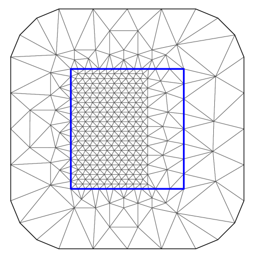
Figure 2: Triangulation for the shot data locations over which the “tent” functions are constructed (black line), and the observation locations are inside the blue rectangle.

Based on INLA, we obtain estimated intensity surfaces $\widehat{\lambda}^{(1)}(\cdot),\widehat{\lambda}^{(2)}(\cdot),\ldots,\widehat{\lambda}^{(n)}(\cdot)$, and then obtain $\mathscr{S}$ by (4) and (6). Next, we use MFM-PPGrouping for group learning based on $\mathscr{S}$. The sampler presented in Algorithm 1 is used to sample from the posterior distributions for unknown parameters, including $k$, $z=(z_{1},\ldots,z_{n})\in\{1,\ldots,k\}^{n}$ and $\lambda=(\lambda_{1},\ldots,\lambda_{n})$ in (3.2). As it marginalizes over the distribution of $k$, the sampler does not depend on reversible jump, and is more efficient than allocation samplers.

Algorithm 1 Collapsed Sampler for MFM-PPGrouping

1:procedure c-MFM-PPGrouping

2:Initialize: let $\bm{z}=(z_{1},\ldots,z_{n})$, $\bm{U}=(U_{rs})$, $\bm{T}=(T_{rs})$.

3:     for each iter $=1$ to M  do

4:Update $\bm{T}=(T_{rs})$ conditional on $z$ as

$$\begin{split}p(T_{rs}\mid\mathscr{S},z)&\sim\mbox{Gamma}\left(\alpha+n_{rs}/2,\beta+(n_{rs}-1)\text{var}(A_{[rs]})/2+\dfrac{k_{0}n_{rs}(\overline{A}_{[rs]}-\mu_{0})^{2}}{2(k_{0}+n_{rs})}\right)\end{split}$$

5:Update $\bm{U}=(U_{rs})$ conditional on $z$ as

$$\begin{split}p(U_{rs}\mid\mathscr{S},T_{rs},z)&\sim\mbox{N}\left(\dfrac{k_{0}\mu_{0}+n_{rs}\overline{A}_{[rs]}}{k_{0}+n_{rs}},((k_{0}+n_{rs})T_{rs})^{-1}\right)\end{split}$$

where ${A}_{[rs]}=(\mathscr{S}_{ij};{z_{i}=r,z_{j}=s,i\neq j})$, $\overline{A}_{[rs]}=(\sum_{z_{i}=r,z_{j}=s,i\neq j}\mathscr{S}_{ij})/n_{rs}$ and $n_{rs}=\sum_{i\neq j}I(z_{i}=r,z_{j}=s),r=1,\ldots,k;s=1,\ldots,k$. Note that $k$ denotes the number of groups yielded by the current $z$.

6:Update $\bm{z}=(z_{1},\ldots,z_{n})$ conditional on $\bm{U}=(U_{rs})$ and $\bm{T}=(T_{rs})$. For each $i$ in $(1,\ldots,n)$, $P(z_{i}=c\mid z_{-i},\mathscr{S},U,T)$ can be obtained in closed form as:

$$\propto\left\{\begin{array}[]{ll}[\absolutevalue{c}+\gamma][\prod_{j>i}\frac{1}{\sqrt{2\pi T_{cz_{j}}^{-1}}}e^{-\frac{T_{cz_{j}}(\mathscr{S}_{ij}-U_{cz_{j}})^{2}}{2}}][\prod_{k<i}\frac{1}{\sqrt{2\pi T_{z_{k}c}^{-1}}}e^{-\frac{T_{z_{k}c}(\mathscr{S}_{ki}-U_{z_{k}c})^{2}}{2}}]&\text{at an existing table $c$}\\ \frac{V_{n}(\absolutevalue{\mathcal{C}_{-i}}+1)}{V_{n}(\absolutevalue{\mathcal{C}_{-i}}}\gamma m(\mathscr{S}_{i})&\text{if $c$ is a new table}\\ \end{array},\right.$$

with $\mathcal{C}_{-i}$ being the partition obtained by removing $z_{i}$ and

$$m(\mathscr{S}_{i})=\prod_{t=1}^{\absolutevalue{\mathcal{C}_{-i}}}\dfrac{\Gamma(\alpha_{n})}{\Gamma(\alpha)}\dfrac{\beta^{\alpha}}{\beta_{n}^{\alpha_{n}}}\left(\frac{k_{0}}{k_{0}+n_{t}}\right)^{\frac{1}{2}}(2\pi)^{\frac{-n_{t}}{2}},$$

where $\alpha_{n}=\alpha+n_{t}/2$, $n_{t}=\sum_{i\neq j}I(z_{j}=t)$, $\beta_{n}=\beta+(n_{t}-1)\text{var}(A_{[t]})/2+\dfrac{k_{0}n_{t}(\overline{A}_{[t]}-\mu_{0})^{2}}{2(k_{0}+n_{t})}$, ${A}_{[t]}=(\mathscr{S}_{ij};{z_{j}=t,i\neq j})$ and $\overline{A}_{[t]}=(\sum_{z_{j}=t,i\neq j}\mathscr{S}_{ij})/n_{t}$.

7:     end for

8:end procedure

After obtaining posterior samples of $\{z_{1},z_{2},\ldots,z_{n}\}$, posterior inference for the group configurations needs to be carried out so that the values are nominal integers denoting group belongings. This renders the posterior mean unsuitable for our purpose. We adopt Dahl’s method (Dahl, 2006). Define a membership matrix $\mathcal{B}^{(\ell)}$ as:

$$\begin{split}\mathcal{B}^{(\ell)}=(\mathcal{B}^{(\ell)}(i,j))_{i,j\in\{1:n\}}=(z_{i}^{(\ell)}=z_{j}^{(\ell)})_{n\times n},\end{split}$$ (16)

where $\ell=1,\ldots,B$ indexes the number of post-burnin MCMC iterations, $z_{i}^{(\ell)}$ and $z_{j}^{(\ell)}$ denote the memberships for players $i$ and $j$, respectively. An entry $\mathcal{B}^{(\ell)}(i,j)$ equals 1 if $z_{i}^{(\ell)}=z_{j}^{(\ell)}$, and 0 otherwise. An element-wise mean of the membership matrices can be obtained as

$$\overline{\mathcal{B}}=\frac{1}{B}\sum_{t=1}^{B}\mathcal{B}^{(t)},$$

where the summation is also element-wise. The posterior iteration with the smallest squared distance to $\overline{\mathcal{B}}$ is obtained by

$$C_{LS}=\text{argmin}_{c\in(1:B)}\sum_{i=1}^{n}\sum_{j=1}^{n}(\mathcal{B}^{(c)}(i,j)-\overline{\mathcal{B}}(i,j))^{2}.$$ (17)

The estimated parameters, together with the group assignments $\bm{z}$, are obtained from $C_{LS}$th post burn-in iteration. With the Dahl’s method, our Bayesian grouping method is summarized in Algorithm 2.

Algorithm 2 Bayesian Group Learning Procedure for Basketball Players

1:Fit LGCPs for $n$ different players $\bm{y}^{(1)},\bm{y}^{(2)},\ldots,\bm{y}^{(n)}$ via inlabru and get $n$ underlying intensity surface $\widehat{\lambda}^{(1)}(\cdot),\widehat{\lambda}^{(2)}(\cdot),\ldots,\widehat{\lambda}^{(n)}(\cdot)$,

2:Use (4) and (5) to construct matrix $\bm{S}$ and matrix $\mathscr{S}$ and based on $\widehat{\lambda}^{(1)}(\cdot),\widehat{\lambda}^{(2)}(\cdot),\ldots,\widehat{\lambda}^{(n)}(\cdot)$,

3:Get $B$ posterior samples of $\bm{z}^{(1)},\bm{z}^{(2)},\ldots,\bm{z}^{(B)}$ from $\mathscr{S}$ via Algorithm 1,

4:Summary posterior samples by Dahl’s method.

5 Simulation

5.1 Simulation Setup

A total of three groups are designed, each of which has its own base intensity as shown in Figure 3. The first group corresponds to players most of whose shots are in the painted area; the second group corresponds to players whose shot locations are widely distributed in every location from painted area to three-point line. A player in the third group has more shot at the three-point line and inside the painted area. To create some variation between players within the same group so that their shot charts are not generated from exactly the same intensity surface, a noise term has been added to the base surfaces, so that for player $i$ in group $k$,

$$\lambda_{k,i}(\cdot)=\lambda_{k}(\cdot)+|\bm{\epsilon}_{k,i}|,~{}~{}k=1,2,3,~{}~{}i=1,\ldots,25,$$ (18)

where $\lambda_{k}(\cdot)$ denote the three base intensity surfaces in Figure 3, $\bm{\epsilon}_{k,i}$ is generated from a multivariate normal distribution with mean $\bm{0}$ and variance $0.5\textbf{I}$, and an absolute value step is taken to ensure that the summation produces a positive and valid intensity surface.

With 75 valid intensity surfaces having both between group variation and within group variation, shot locations for the 75 players are generated following the Poisson process as in Equation (2). Algorithm 2 is implemented on these 75 players, and we examine both the estimation for number of groups as well as congruence of group belongings with the true setting in terms of modulo labeling by Rand index (RI; Rand, 1971), the computation of which is facilitated by the R-package fossil (Vavrek, 2011). The RI ranges from 0 to 1 with a higher value indicating better agreement between a grouping scheme and the true setting. In particular, a value of 1 indicates perfect agreement.

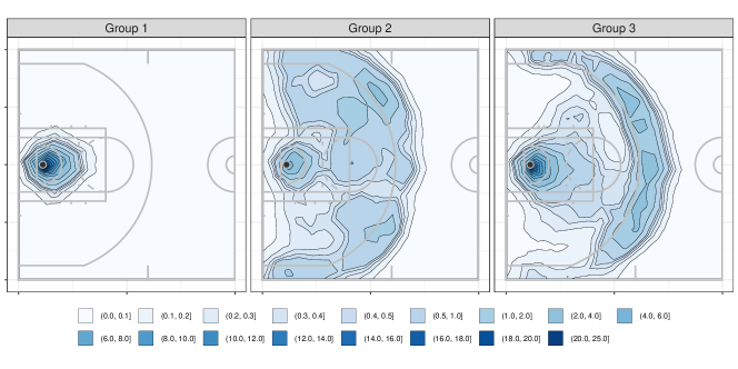
Figure 3: Visualization of three bases for the three groups in simulation design.

5.2 Simulation Results

We run our algorithm with 1,000 MCMC iterations, with the first 500 iterations as burn-in for each replicate data. We examine it is sufficient for the chain to converge and stabilize. The numbers are chosen to be sufficiently large for the chain to converge and stabilize. To verify this, with a single replicate of data, 50 separate MCMC chains are run with different random seeds and hence initial values, and 50 final grouping schemes are obtained. The RI is calculated for these 50 chains at each of their iteration, giving 50 traces, which are visualized in Figure 4. It can be observed that covergence is attained after a small number of iterations, and the band of the 50 traces is rather tight after convergence.

Proceeding to 50 separate replicates of data, our proposed algorithm was run, and 50 RI values are obtained by comparing with the true setting. They average to 0.9988, which indicates rather accurate grouping ability of the proposed approach. In addition, performance comparisons of our proposed method with three competing methods are made. We compare our method to K-means algorithm, Density-based spatial grouping of applications with noise (DBSCAN) and mean shift grouping. Grouping recovery performances of all four methods are measured using the RI. The 50 final RI’s obtained for the three competitors average to 0.9005, 0.7642, and 0.7380, respectively, indicating the superior performance of our proposed approach. We also show the number of cluster covered by our algorithm, see Figure 5. We see that there are fourty two replicates have three clusters.

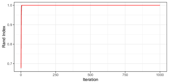
Figure 4: Rand Index trace plot for single replicate simulated data. Dark grey line indicates for each random seed. Red line is the average rand index for 50 random seeds.

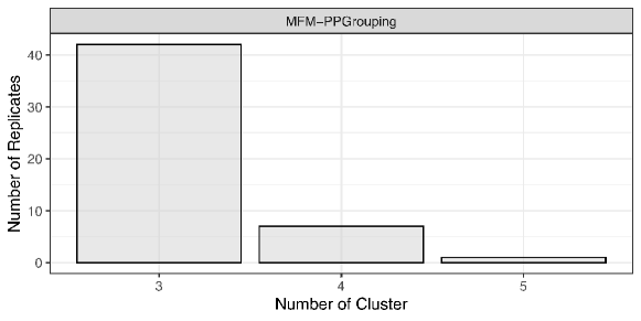
Figure 5: Histogram for the number of clusters produced by MFM-PPGrouping in 50 simulation replicates.

6 Analysis of NBA Players

In this section, we apply the proposed method to the analysis of players’ shot data in the 2017-2018 NBA regular season. Only the locations of shots are considered regardless of the players’ positions on the court (e.g., point guard, power forward, etc.). Players’ positions (e.g., point guard, power forward, etc) are not considered, but only the shots’ positions. As a starting point, a predictive intensity matrix is obtained for each player using inlabru. Algorithms 1 and 2 are subsequently used to identify the groups. We run 1,000 MCMC iterations and the first 500 iterations as burn-in period. The result from the MFM model suggests that the 191 players are to be classified into nine groups. The sizes of the nine groups are 10, 59, 8, 19, 24, 8, 10, 51, and 2 respectively. Visualizations of intensity matrices with contour for two selected players from each group are presented in Figure 6.

Several interesting observations can be made from the visualization results. First, we discuss groups 1, 3 and 9. The contours for group 1 and group 3 are wider than the contours for group 9, where most shots are located near the hoop. Clint Capela and DeAndre Jordan (in group 9), for example, are both good at making alley-oops and slam dunks. Only very few shots are made by these players outside the painted area. Despite the similarity between groups 1 and 3, it can be seen that for group 3, most of the shots are made within the painted area, while there are quite a number of shots outside the painted area for group 1, indicating wider shooting ranges for the corresponding players.

Groups 4 and 7 share some characteristic in common as most of the shot locations are around the hoop. Players in group 4, however, are also able to shoot frequently beyond the three-point line at a wider range of angles, while players in group 7 also shoot beyond the three-point line at very limited angles.

Groups 2, 5 and 8 also bear some resemblance with each other. A first look at the fitted intensity contours indicates that players in these groups are able to make all types of shots, including three-pointers, perimeter shot, and also shots over the painted area. Group 2 is differentiated from the other two as most of the shots are made around the hoop, and the intensity for perimeter shots and three-pointers are rather similar. For group 5, however, the intensity for shots around the hoop is much lower than that for group 2. For group 8, players make most shots around the hoop and also make some perimeter shots as well as three-pointers. Compared with the other two groups, they have a more narrow range of angles to make perimeter shots and three-pointers. Most shots are located between 45 degrees up and down angle from the horizontal line across the hoop.

Group 6 has little similarity with any other groups. As can be seen, most shots are located either near the hoop, or beyond the three-point line. There are very few perimeter shots. Kyle Korver and Nick Young, both of whom are well-known catch-and-release shooters, fall in this group.

As further verification, we use multidimensional scaling to lower the dimension of the fitted intensity matrices for players to 2 so that similarities in their shooting habits can be visualized. See Figure 7. Separation of the nine groups is quite clear. Group 9, for example, with its unique strong preference for alley-oops and slam dunks, stands far from others.

Finally, to make sure the group configuration presented here is not a random occurrence but reflects the true pattern demonstrated by the data, we run 50 separate MCMC chains with different random seeds and initial values, and obtained 50 final grouping schemes. The RI between each scheme and the present grouping scheme is calculated, and they average to 0.948, indicating high concordance of conclusion regardless of random seeds.

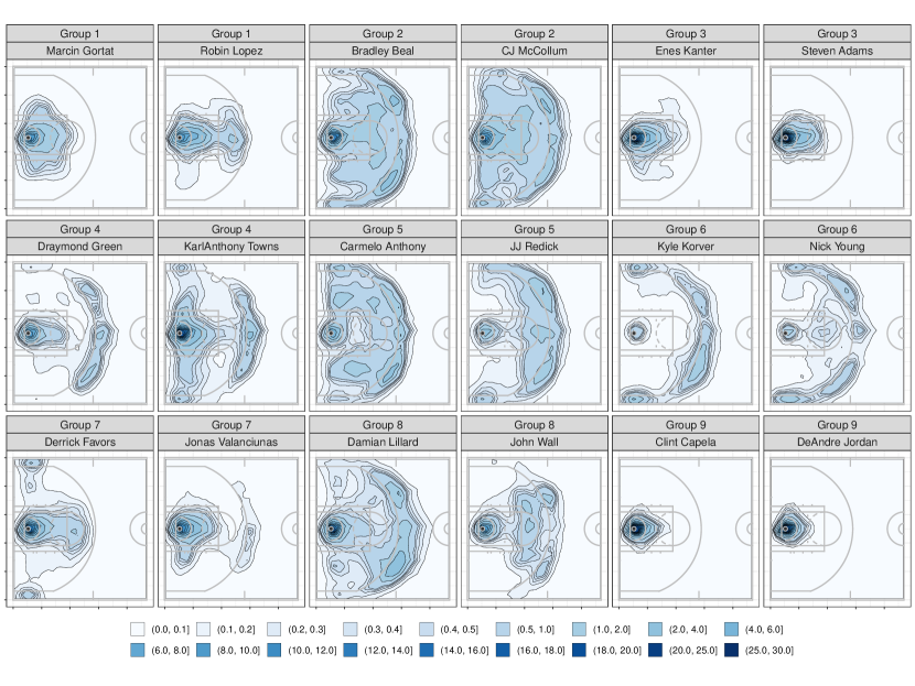
Figure 6: Fitted intensities with contour lines for two selected players in each of the nine identified groups.

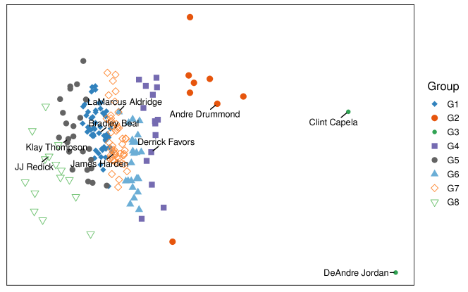
Figure 7: Visualization of the night identified groups of players, with selected players’ names annotated.

7 Conclusion

In this paper, we proposed using MFM to capture heterogeneity of different NBA players based on LGCP. Our group learning method provides a quantitative summary of different players shot habits other than traditional position categorization. Our simulation results indicated that our proposed methods achieve good grouping accuracy.

The real data application give us the information about player’s shooting habit location. Players can understand their own shooting habits, and they can also strengthen their weaker shooting locations. On the other hand, the professional coach can formulate a defensive strategy to reduce the opponent’s score with these information. Our grouping results will provide a good guidance for team managers trading the players with similar shot pattern.

A few topics beyond the scope of this paper are worth further investigation. In this paper, a two-stage group learning method is proposed. An unified approach is an interesting alternative in future work. In addition, incorporating auxiliary information such as player position or historical information could also be taken into account for grouping in our future work. Jointly modeling spatial field goal percentage and shot selection will provide more detail instructions for professional coaches.

References

- Aldous (1985) Aldous, D. J. (1985). Exchangeability and related topics. In École d’Été de Probabilités de Saint-Flour XIII-1983, pp. 1–198. Springer.
- Antoniak (1974) Antoniak, C. E. (1974). Mixtures of Dirichlet processes with applications to Bayesian nonparametric problems. The Annals of Statistics 2(6), 1152–1174.
- Bachl et al. (2019) Bachl, F. E., F. Lindgren, D. L. Borchers, and J. B. Illian (2019). inlabru: an R package for Bayesian spatial modelling from ecological survey data. Methods in Ecology and Evolution 10(6), 760–766.
- Blackwell et al. (1973) Blackwell, D., J. B. MacQueen, et al. (1973). Ferguson distributions via Pólya urn schemes. The Annals of Statistics 1(2), 353–355.
- Cervone et al. (2016) Cervone, D., A. D’Amour, L. Bornn, and K. Goldsberry (2016). A multiresolution stochastic process model for predicting basketball possession outcomes. Journal of the American Statistical Association 111(514), 585–599.
- Chen et al. (2019) Chen, Y., R. Pan, R. Guan, and H. Wang (2019). A case study for Beijing point of interest data using group linked Cox process. Statistics and Its Interface 12(2), 331–344.
- Dahl (2006) Dahl, D. B. (2006). Model-based clustering for expression data via a Dirichlet process mixture model. In M. V. Kim-Anh Do, Peter Müller (Ed.), Bayesian Inference for Gene Expression and Proteomics, Volume 4, pp. 201–218. Cambridge University Press.
- Diggle et al. (1976) Diggle, P. J., J. Besag, and J. T. Gleaves (1976). Statistical analysis of spatial point patterns by means of distance methods. Biometrics 3(32), 659–667.
- Diggle et al. (2007) Diggle, P. J., V. Gómez-Rubio, P. E. Brown, A. G. Chetwynd, and S. Gooding (2007). Second-order analysis of inhomogeneous spatial point processes using case–control data. Biometrics 63(2), 550–557.
- Ferguson (1973) Ferguson, T. S. (1973). A Bayesian analysis of some nonparametric problems. The Annals of Statistics 1(2), 209–230.
- Franks et al. (2015) Franks, A., A. Miller, L. Bornn, and K. Goldsberry (2015). Characterizing the spatial structure of defensive skill in professional basketball. The Annals of Applied Statistics 9(1), 94–121.
- Geng et al. (2019) Geng, J., A. Bhattacharya, and D. Pati (2019). Probabilistic community detection with unknown number of communities. Journal of the American Statistical Association 114(526), 893–905.
- Geng et al. (2019) Geng, J., W. Shi, and G. Hu (2019). Bayesian nonparametric nonhomogeneous Poisson process with applications to USGS earthquake data. arXiv preprint arXiv:1907.03186.
- Geyer (1998) Geyer, C. (1998). Likelihood inference for spatial point processes. In W. S. Kendall (Ed.), Stochastic Geometry: Likelihood and Computation, Volume 80, pp. 79. CRC Press.
- Goulard et al. (1996) Goulard, M., A. Särkkä, and P. Grabarnik (1996). Parameter estimation for marked Gibbs point processes through the maximum pseudo-likelihood method. Scandinavian Journal of Statistics 23(3), 365–379.
- Guan (2008) Guan, Y. (2008). On consistent nonparametric intensity estimation for inhomogeneous spatial point processes. Journal of the American Statistical Association 103(483), 1238–1247.
- Hu et al. (2019) Hu, G., F. Huffer, and M.-H. Chen (2019). New development of Bayesian variable selection criteria for spatial point process with applications. arXiv preprint arXiv:1910.06870.
- Jiao et al. (2019) Jiao, J., G. Hu, and J. Yan (2019). A Bayesian joint model for spatial point processes with application to basketball shot chart. arXiv preprint arXiv:1908.05745.
- Jiao et al. (2020) Jiao, J., G. Hu, and J. Yan (2020). Heterogeneity pursuit for spatial point pattern with application to tree locations: A Bayesian semiparametric recourse. arXiv preprint arXiv:2003.10043.
- Lindgren et al. (2011) Lindgren, F., H. Rue, and J. Lindström (2011). An explicit link between Gaussian fields and Gaussian Markov random fields: the stochastic partial differential equation approach. Journal of the Royal Statistical Society: Series B (Statistical Methodology) 73(4), 423–498.
- Miller et al. (2014) Miller, A., L. Bornn, R. Adams, and K. Goldsberry (2014). Factorized point process intensities: A spatial analysis of professional basketball. In E. P. Xing and T. Jebara (Eds.), Proceedings of the 31st International Conference on Machine Learning, Volume 32 of Proceedings of Machine Learning Research, Bejing, China, pp. 235–243. PMLR.
- Miller and Harrison (2013) Miller, J. W. and M. T. Harrison (2013). A simple example of Dirichlet process mixture inconsistency for the number of components. In C. J. C. Burges, L. Bottou, M. Welling, Z. Ghahramani, and K. Q. Weinberger (Eds.), Advances in Neural Information Processing Systems 26, pp. 199–206. Curran Associates, Inc.
- Miller and Harrison (2018) Miller, J. W. and M. T. Harrison (2018). Mixture models with a prior on the number of components. Journal of the American Statistical Association 113(521), 340–356.
- Møller et al. (1998) Møller, J., A. R. Syversveen, and R. P. Waagepetersen (1998). Log Gaussian Cox processes. Scandinavian Journal of Statistics 25(3), 451–482.
- Neal (2000) Neal, R. M. (2000). Markov chain sampling methods for Dirichlet process mixture models. Journal of Computational and Graphical Statistics 9(2), 249–265.
- Pitman (1995) Pitman, J. (1995). Exchangeable and partially exchangeable random partitions. Probability Theory and Related Fields 102(2), 145–158.
- Rand (1971) Rand, W. M. (1971). Objective criteria for the evaluation of clustering methods. Journal of the American Statistical Association 66(336), 846–850.
- Rasmussen and Williams (2006) Rasmussen, C. E. and C. K. Williams (2006). Gaussian Processes for Machine Learning. MIT Press Cambridge, MA.
- Reich et al. (2006) Reich, B. J., J. S. Hodges, B. P. Carlin, and A. M. Reich (2006). A spatial analysis of basketball shot chart data. The American Statistician 60(1), 3–12.
- Rue et al. (2009) Rue, H., S. Martino, and N. Chopin (2009). Approximate Bayesian inference for latent gaussian models by using integrated nested Laplace approximations. Journal of the royal statistical society: Series b (statistical methodology) 71(2), 319–392.
- Simpson et al. (2016) Simpson, D., J. B. Illian, F. Lindgren, S. H. Sørbye, and H. Rue (2016). Going off grid: Computationally efficient inference for log-Gaussian Cox processes. Biometrika 103(1), 49–70.
- Simpson et al. (2017) Simpson, D., H. Rue, A. Riebler, T. G. Martins, S. H. Sørbye, et al. (2017). Penalising model component complexity: A principled, practical approach to constructing priors. Statistical Science 32(1), 1–28.
- Thurman et al. (2015) Thurman, A. L., R. Fu, Y. Guan, and J. Zhu (2015). Regularized estimating equations for model selection of clustered spatial point processes. Statistica Sinica 25(1), 173–188.
- Vavrek (2011) Vavrek, M. J. (2011). fossil: palaeoecological and palaeogeographical analysis tools. Palaeontologia Electronica 14(1), 1T. R package version 0.4.0.
- Veen and Schoenberg (2006) Veen, A. and F. P. Schoenberg (2006). Assessing spatial point process models using weighted K-functions: analysis of California earthquakes, pp. 293–306. New York, NY: Springer New York.