A Generative Model for Joint
Natural Language Understanding and Generation

Abstract

Natural language understanding (NLU) and natural language generation (NLG) are two fundamental and related tasks in building task-oriented dialogue systems with opposite objectives: NLU tackles the transformation from natural language to formal representations, whereas NLG does the reverse. A key to success in either task is parallel training data which is expensive to obtain at a large scale. In this work, we propose a generative model which couples NLU and NLG through a shared latent variable. This approach allows us to explore both spaces of natural language and formal representations, and facilitates information sharing through the latent space to eventually benefit NLU and NLG. Our model achieves state-of-the-art performance on two dialogue datasets with both flat and tree-structured formal representations. We also show that the model can be trained in a semi-supervised fashion by utilising unlabelled data to boost its performance.

1 Introduction

Natural language understanding (NLU) and natural language generation (NLG) are two fundamental tasks in building task-oriented dialogue systems. In a modern dialogue system, an NLU module first converts a user utterance, provided by an automatic speech recognition model, into a formal representation. The representation is then consumed by a downstream dialogue state tracker to update a belief state which represents an aggregated user goal. Based on the current belief state, a policy network decides the formal representation of the system response. This is finally used by an NLG module to generate the system responseYoung et al. (2010).

It can be observed that NLU and NLG have opposite goals: NLU aims to map natural language to formal representations, while NLG generates utterances from their semantics. In research literature, NLU and NLG are well-studied as separate problems. State-of-the-art NLU systems tackle the task as classification Zhang and Wang (2016) or as structured prediction or generation Damonte et al. (2019), depending on the formal representations which can be flat slot-value pairs Henderson et al. (2014), first-order logical form Zettlemoyer and Collins (2012), or structured queries Yu et al. (2018); Pasupat et al. (2019). On the other hand, approaches to NLG vary from pipelined approach subsuming content planning and surface realisation Stent et al. (2004) to more recent end-to-end sequence generation Wen et al. (2015); Dušek et al. (2020).

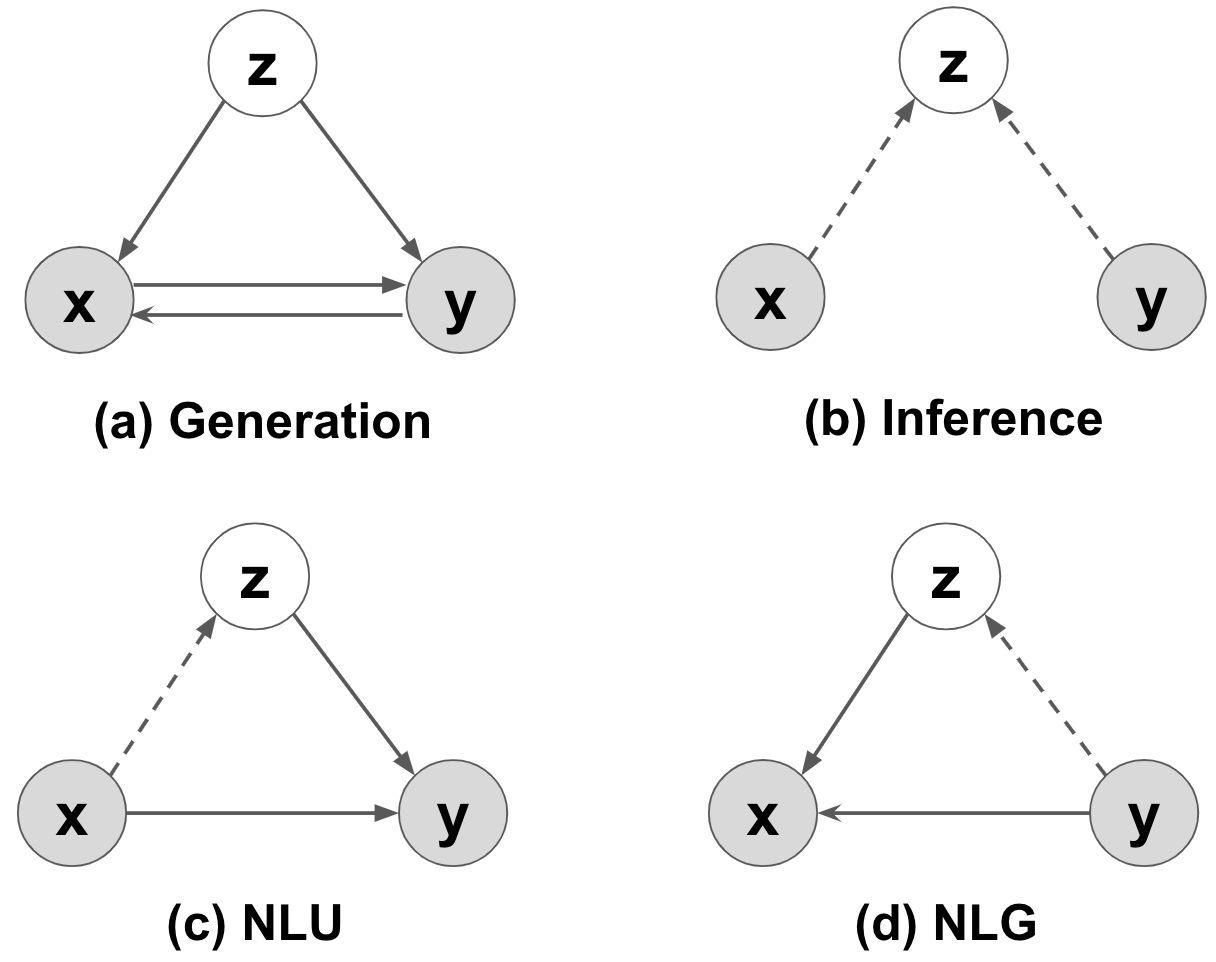
Figure 1: Generation and inference process in our model, and how NLU and NLG are achieved. $x$ and $y$ denotes utterances and formal representations respectively; $z$ represents the shared latent variable for $x$ and $y$.

However, the duality between NLU and NLG has been less explored. In fact, both tasks can be treated as a translation problem: NLU converts natural language to formal language while NLG does the reverse. Both tasks require a substantial amount of utterance and representation pairs to succeed, and such data is costly to collect due to the complexity of annotation involved. Although unannotated data for either natural language or formal representations can be easily obtained, it is less clear how they can be leveraged as the two languages stand in different space.

In this paper, we propose a generative model for Joint natural language Understanding and Generation (JUG), which couples NLU and NLG with a latent variable representing the shared intent between natural language and formal representations. We aim to learn the association between two discrete spaces through a continuous latent variable which facilitates information sharing between two tasks. Moreover, JUG can be trained in a semi-supervised fashion, which enables us to explore each space of natural language and formal representations when unlabelled data is accessible. We examine our model on two dialogue datasets with different formal representations: the E2E dataset Novikova et al. (2017) where the semantics are represented as a collection of slot-value pairs; and a more recent weather dataset Balakrishnan et al. (2019) where the formal representations are tree-structured. Experimental results show that our model improves over standalone NLU/NLG models and existing methods on both tasks; and the performance can be further boosted by utilising unlabelled data.

2 Model

Our key assumption is that there exists an abstract latent variable $z$ underlying a pair of utterance $x$ and formal representation $y$. In our generative model, this abstract intent guides the standard conditional generation of either NLG or NLU (Figure 1a). Meanwhile, $z$ can be inferred from either utterance $x$, or formal representation $y$ (Figure 1b). That means performing NLU requires us to infer the $z$ from $x$, after which the formal representation $y$ is generated conditioning on both $z$ and $x$ (Figure 1c), and vice-versa for NLG (Figure 1d). In the following, we will explain the model details, starting with NLG.

2.1 NLG

As mentioned above, the task of NLG requires us to infer $z$ from $y$, and then generate $x$ using both $z$ and $y$. We choose the posterior distribution $q(z|y)$ to be Gaussian. The task of inferring $z$ can then be recast to computing mean $\mu$ and standard deviation $\sigma$ of the Gaussian distribution using an NLG encoder. To do this, we use a bi-directional LSTM Hochreiter and Schmidhuber (1997) to encode formal representation $y$. which is linearised and represented as a sequence of symbols. After encoding, we obtain a list of hidden vectors $\mathbf{H}$, with each representing the concatenation of forward and backward LSTM states. These hidden vectors are then average-pooled and passed through two feed-forward neural networks to compute mean $\boldsymbol{\mu}_{y,z}$ and standard deviation $\boldsymbol{\sigma}_{y,z}$ vectors of the posterior $q(z|y)$.

$$\begin{split}&\mathbf{H}=\text{Bi-LSTM}(\mathbf{y})\\ &\mathbf{\mathbf{\bar{h}}}=\text{Pooling}(\mathbf{H})\\ &\boldsymbol{\mu}_{y,z}=\mathbf{W}_{\mu}\mathbf{\bar{h}}+\mathbf{b}_{\mu}\\ &\boldsymbol{\sigma}_{y,z}=\mathbf{W}_{\sigma}\mathbf{\bar{h}}+\mathbf{b}_{\sigma}\end{split}$$ (1)

where $\mathbf{W}$ and $\mathbf{b}$ represent neural network weights and bias. Then the latent vector $\mathbf{z}$ can be sampled from the approximated posterior using the re-parameterisation trick of Kingma and Welling (2013):

$$\begin{split}&\boldsymbol{\epsilon}\sim\mathcal{N}(0,\mathbf{I})\\ &\mathbf{z}=\boldsymbol{\mu}_{y,z}+\boldsymbol{\sigma}_{y,z}\boldsymbol{\epsilon}\end{split}$$ (2)

The final step is to generate natural language $x$ based on latent variable $z$ and formal representation $y$. We use an LSTM decoder relying on both $z$ and $y$ via attention mechanism Bahdanau et al. (2014). At each time step, the decoder computes:

$$\begin{split}&\mathbf{g}_{i}^{x}=\text{LSTM}(\mathbf{g}_{i-1}^{x},\mathbf{x}_{i-1})\\ &\mathbf{c}_{i}=\text{attention}(\mathbf{g}_{i}^{x},\mathbf{H})\\ &p(x_{i})=\text{softmax}(\mathbf{W_{v}}[\mathbf{c}_{i}\oplus\mathbf{g}_{i}^{x}\oplus\mathbf{z}]+\mathbf{b}_{v})\end{split}$$ (3)

where $\oplus$ denotes concatenation. $\mathbf{x}_{i-1}$ is the word vector of input token; $\mathbf{g}_{i}^{x}$ is the corresponding decoder hidden state and $p(x_{i})$ is the output token distribution at time step $i$.

2.2 NLU

NLU performs the reverse procedures of NLG. First, an NLU encoder infers the latent variable $z$ from utterance $x$. The encoder uses a bi-directional LSTM to convert the utterance into a list of hidden states. These hidden states are pooled and passed through feed-forward neural networks to compute the mean $\boldsymbol{\mu}_{x,z}$ and standard deviation $\boldsymbol{\sigma}_{x,z}$ of the posterior $q(z|x)$. This procedure follows Equation LABEL:eq:nlg-enc in NLG.

However, note that a subtle difference between natural language and formal language is that the former is ambiguous while the later is precisely defined. This makes NLU a many-to-one mapping problem but NLG is one-to-many. To better reflect the fact that the NLU output requires less variance, when decoding we choose the latent vector $\mathbf{z}$ in NLU to be the mean vector $\boldsymbol{\mu}_{x,z}$, instead of sampling it from $q(z|x)$ like Equation 2.

After the latent vector is obtained, the formal representation $y$ is predicted from both $z$ and $x$ using an NLU decoder. Since the space of $y$ depends on the formal language construct, we consider two common scenarios in dialogue systems. In the first scenario, $y$ is represented as a set of slot-value pairs, e.g., {food type=British, area=north} in restaurant search domain Mrkšić et al. (2017). The decoder here consists of several classifiers, one for each slot, to predict the corresponding values. Each classifier is modelled by a 1-layer feed-forward neural network that takes $z$ as input:

$$\begin{split}&p(y_{s})=\text{softmax}(\mathbf{W_{s}}\mathbf{z}+\mathbf{b_{s}})\\ \end{split}$$ (4)

where $p(y_{s})$ is the predicted value distribution of slot $s$.

In the second scenario, $y$ is a tree-structured formal representation Banarescu et al. (2013). We then generate $y$ as a linearised token sequence using an LSTM decoder relying on both $z$ and $x$ via the standard attention mechanism Bahdanau et al. (2014). The decoding procedure follows exactly Equation 3.

2.3 Model Summary

One flexibility of the JUG model comes from the fact that it has two ways to infer the shared latent variable $z$ through either $x$ or $y$; and the inferred $z$ can aid the generation of both $x$ and $y$. In this next section, we show how this shared latent variable enables the JUG model to explore unlabelled $x$ and $y$, while aligning the learned meanings inside the latent space.

3 Optimisation

We now describe how JUG can be optimised with a pair of $x$ and $y$ (§3.1), and also unpaired $x$ or $y$ (§3.2). We specifically discuss the prior choice of JUG objectives in §3.3. A combined objective can be thus derived for semi-supervised learning: a practical scenario when we have a small set of labelled data but abundant unlabelled ones (§3.4).

3.1 Optimising $p(x,y)$

Given a pair of utterance $x$ and formal representation $y$, our objective is to maximise the log-likelihood of the joint probability $p(x,y)$:

$$\log p(x,y)=\log\int_{z}p(x,y,z)$$ (5)

The optimisation task is not directly tractable since it requires us to marginalise out the latent variable $z$. However, it can be solved by following the standard practice of neural variational inference Kingma and Welling (2013). An objective based on the variational lower bound can be derived as

$$\begin{split}\mathcal{L}_{x,y}&=\mathbb{E}_{q(z|x)}\log p(y|z,x)+\mathbb{E}_{q(z|x)}\log p(x|z,y)\\ &\,\,\,\,\,-\text{KL}[q(z|x)||p(z)]\end{split}$$ (6)

where the first term on the right side is the NLU model; the second term is the reconstruction of $x$; and the last term denotes the Kullback$-$Leibler divergence between the approximate posterior $q(z|x)$ with the prior $p(z)$. We defer the discussion of prior to Section 3.3 and detailed derivations to Appendix.

The symmetry between utterance and semantics offers an alternative way of inferring the posterior through the approximation $q(z|y)$. Analogously we can derive a variational optimisation objective:

$$\begin{split}\mathcal{L}_{y,x}&=\mathbb{E}_{q(z|y)}\log p(x|z,y)+\mathbb{E}_{q(z|y)}\log p(y|z,x)\\ &\,\,\,\,\,-\text{KL}[q(z|y)||p(z)]\end{split}$$ (7)

where the first term is the NLG model; the second term is the reconstruction of $y$; and the last term denotes the KL divergence.

It can be observed that our model has two posterior inference paths from either $x$ or $y$, and also two generation paths. All paths can be optimised.

3.2 Optimising $p(x)$ or $p(y)$

Additionally, when we have access to unlabelled utterance $x$ (or formal representation $y$), the optimisation objective of JUG is the marginal likelihood $p(x)$ (or $p(y)$):

$$\log p(x)=\log\int_{y}\int_{z}p(x,y,z)$$ (8)

Note that both $z$ and $y$ are unobserved in this case.

We can develop an objective based on the variational lower bound for the marginal:

$$\begin{split}\mathcal{L}_{x}&=\mathbb{E}_{q(y|z,x)}\mathbb{E}_{q(z|x)}\log p(x|z,y)\\ &\,\,-\text{KL}[q(z|x)||p(z)]\end{split}$$ (9)

where the first term is the auto-encoder reconstruction of $x$ with a cascaded NLU-NLG path. The second term is the KL divergence which regularizes the approximated posterior distribution. Detailed derivations can be found in Appendix.

When computing the reconstruction term of $x$, it requires us to first run through the NLU model to obtain the prediction on $y$, from which we run through NLG to reconstruct $x$. The full information flow is ($x\rightarrow z\rightarrow y\rightarrow z\rightarrow x$). Connections can be drawn with recent work which uses back-translation to augment training data for machine translation Sennrich et al. (2016); He et al. (2016). Unlike back-translation, the presence of latent variable in our model requires us to sample $z$ along the NLU-NLG path. The introduced stochasticity allows the model to explore a larger area of the data manifold.

The above describes the objectives when we have unlabelled $x$. We can derive a similar objective for leveraging unlabelled $y$:

$$\begin{split}\mathcal{L}_{y}&=\mathbb{E}_{q(x|z,y)}\mathbb{E}_{q(z|y)}\log p(y|z,x)\\ &\,\,-\text{KL}[q(z|y)||p(z)]\end{split}$$ (10)

where the first term is the auto-encoder reconstruction of $y$ with a cascaded NLG-NLU path. The full information flow here is ($y\rightarrow z\rightarrow x\rightarrow z\rightarrow y$).

3.3 Choice of Prior

The objectives described in 3.1 and 3.2 require us to match an approximated posterior (either $q(z|x)$ or $q(z|y)$) to a prior $p(z)$ that reflects our belief. A common choice of $p(z)$ in the research literature is the Normal distribution Kingma and Welling (2013). However, it should be noted that even if we match both $q(z|x)$ and $q(z|y)$ to the same prior, it does not guarantee that the two inferred posteriors are close to each other; this is a desired property of the shared latent space.

To better address the property, we propose a novel prior choice: when the posterior is inferred from $x$ (i.e., $q(z|x)$), we choose the parameterised distribution $q(z|y)$ as our prior belief of $p(z)$. Similarly, when the posterior is inferred from $y$ (i.e., $q(z|y)$), we have the freedom of defining $p(z)$ to be $q(z|x)$. This approach directly pulls $q(z|x)$ and $q(z|y)$ closer to ensure a shared latent space.

Finally, note that it is straightforward to compute both $q(z|x)$ and $q(z|y)$ when we have parallel $x$ and $y$. However when we have the access to unlabelled data, as described in Section 3.2, we can only use the pseudo $x$-$y$ pairs that are generated by our NLU or NLG model, such that we can match an inferred posterior to a pre-defined prior reflecting our belief of the shared latent space.

3.4 Training Summary

In general, JUG subsumes the following three training scenarios which we will experiment with.

When we have fully labelled $x$ and $y$, the JUG jointly optimises NLU and NLG in a supervised fashion with the objective as follows:

$$\mathcal{L}_{basic}=\sum_{(x,y)\sim(X,Y)}(\mathcal{L}_{x,y}+\mathcal{L}_{y,x})$$ (11)

where $(X,Y)$ denotes the set of labelled examples.

Additionally in the fully supervised setting, JUG can be trained to optimise both NLU, NLG and auto-encoding paths. This corresponds to the following objective:

$$\mathcal{L}_{marginal}=\mathcal{L}_{basic}+\sum_{(x,y)\sim(X,Y)}(\mathcal{L}_{x}+\mathcal{L}_{y})$$ (12)

Furthermore, when we have additional unlabelled $x$ or $y$, we optimise a semi-supervised JUG objective as follows:

$$\mathcal{L}_{semi}=\mathcal{L}_{basic}+\sum_{x\sim X}\mathcal{L}_{x}+\sum_{y\sim Y}\mathcal{L}_{y}$$ (13)

where $X$ denotes the set of utterances and $Y$ denotes the set of formal representations.

4 Experiments

We experiment on two dialogue datasets with different formal representations to test the generality of our model. The first dataset is E2E Novikova et al. (2017), which contains utterances annotated with flat slot-value pairs as their semantic representations. The second dataset is the recent weather dataset Balakrishnan et al. (2019), where both utterances and semantics are represented in tree structures. Examples of the two datasets are provided in tables 1 and 2.

Natural Language

"sousa offers british food in the low price range. it is family friendly with a 3 out of 5 star rating. you can find it near the sunshine vegetarian cafe."

Semantic Representation

restaurant_name=sousa, food=english, price_range=cheap, customer_rating=average, family_friendly=yes, near=sunshine vegetarian cafe

Table 1: An example in E2E dataset.

Natural Language (original)

"[__DG_YES__ Yes ] , [__DG_INFORM__ [__ARG_DATE_TIME__ [__ARG_COLLOQUIAL__ today’s ] ] forecast is [__ARG_CLOUD_COVERAGE__ mostly cloudy ] with [__ARG_CONDITION__ light rain showers ] ] ."

Natural Language (processed by removing tree annotations)

"Yes, today’s forecast is mostly cloudy with light rain showers."

Semantic Representation

[__DG_YES__ [__ARG_TASK__ get_weather_attribute ] ] [__DG_INFORM__ [__ARG_TASK__ get_forecast ] [__ARG_CONDITION__ light rain showers ] [__ARG_CLOUD_COVERAGE__ mostly cloudy ] [__ARG_DATE_TIME__ [__ARG_COLLOQUIAL__ today’s ] ] ]

Table 2: An example in weather dataset. The natural language in original dataset (first row) is used for training to have a fair comparison with existing methods. The processed utterances (second row) is used in our semi-supervised setting.

Dataset	Train	Valid	Test
E2E	42061	4672	4693
Weather	25390	3078	3121

Table 3: Number of examples in two datasets

E2E NLU	F1
Dual supervised learning Su et al. (2019)	0.7232
$\textup{JUG}_{\textup{basic}}$	0.7337
E2E NLG	BLEU
TGEN Dušek and Jurcicek (2016)	0.6593
SLUG Juraska et al. (2018)	0.6619
Dual supervised learning Su et al. (2019)	0.5716
$\textup{JUG}_{\textup{basic}}$	0.6855
Weather NLG	BLEU
S2S-CONSTR Balakrishnan et al. (2019)	0.7660
$\textup{JUG}_{\textup{basic}}$	0.7768

Table 4: Comparison with previous systems on two datasets. Note that there is no previous system trained for NLU in weather dataset.

Model / Data	5%	10%	25%	50%	100%
Decoupled	52.77 (0.874)	62.32 (0.902)	69.37 (0.924)	73.68 (0.935)	76.12 (0.942)
$\textup{Augmentation}^{*}$	54.71 (0.878)	62.54 (0.902)	68.91 (0.922)	73.84 (0.935)	-
$\textup{JUG}_{\textup{basic}}$	60.30 (0.902)	67.08 (0.918)	72.49 (0.932)	74.74 (0.937)	78.05 (0.945)
$\textup{JUG}_{\textup{marginal}}$	62.96 (0.907)	68.43 (0.920)	73.35 (0.933)	75.74 (0.939)	78.93 (0.948)
$\textup{JUG}^{*}_{\textup{semi}}$	68.09 (0.921)	70.33 (0.925)	73.79 (0.935)	75.46 (0.939)	-

Table 5: NLU results on E2E dataset. Joint accuracy (%) and F1 score (in bracket) are both reported with varying percentage of labelled training data. Models using unlabelled data are marked with *.

Model / Data	5%	10%	25%	50%	100%
Decoupled	0.693 (83.47)	0.723 (87.33)	0.784 (92.52)	0.793 (94.91)	0.813 (96.98)
$\textup{Augmentation}^{*}$	0.747 (84.79)	0.770 (90.13)	0.806 (94.06)	0.815 (96.04)	-
$\textup{JUG}_{\textup{basic}}$	0.685 (84.20)	0.734 (88.68)	0.769 (93.83)	0.788 (95.11)	0.810 (95.07)
$\textup{JUG}_{\textup{marginal}}$	0.724 (85.57)	0.775 (93.59)	0.803 (94.99)	0.817 (98.67)	0.830 (99.11)
$\textup{JUG}^{*}_{\textup{semi}}$	0.814 (90.47)	0.792 (94.76)	0.819 (95.59)	0.827 (98.42)	-

Table 6: NLG results on E2E dataset. BLEU and semantic accuracy (%) (in bracket) are both reported with varying percentage of labelled training data. Models using unlabelled data are marked with *.

4.1 Training Scenarios

We primarily evaluated our models on the raw splits of the original datasets, which enables us to fairly compare fully-supervised JUG with existing work on both NLU and NLG. Statistics of the two datasets can be found in Table 3.

In addition, we set up an experiment to evaluate semi-supervised JUG with a varying amount of labelled training data (5%, 10%, 25%, 50%, 100%, with the rest being unlabelled). Note that the original E2E test set is designed on purpose with unseen slot-values in the test set to make it difficult Dušek et al. (2018, 2020); we remove the distribution bias by randomly re-splitting the E2E dataset. On the contrary, utterances in the weather dataset contains extra tree-structure annotations which make the NLU task a toy problem. We therefore remove these annotations to make NLU more realistic, as shown in the second row of Table 2.

As described in Section 3.4, we can optimise our proposed JUG model in various ways. We investigate the following approaches:

$\textbf{{JUG}}_{\textbf{{basic}}}$: this model jointly optimises NLU and NLG with the objective in Equation 11. This uses labelled data only.

$\textbf{{JUG}}_{\textbf{{marginal}}}$: jointly optimises NLU, NLG and auto-encoders with only labelled data, per Equation 12.

$\textbf{{JUG}}_{\textbf{{semi}}}$: jointly optimises NLU and NLG with labelled data and auto-encoders with unlabelled data, per Equation 13.

4.2 Baseline Systems

We compare our proposed model with some existing methods as shown in Table 4 and two designed baselines as follows:

Decoupled: The NLU and NLG models are trained separately by supervised learning. Both of the individual models have the same encoder-decoder structure as JUG. However, the main difference is that there is no shared latent variable between the two individual NLU and NLG models.

Augmentation: We pre-train Decoupled models to generate pseudo label from the unlabelled corpus Lee (2013) in a setup similar to back-translation Sennrich et al. (2016). The pseudo data and labelled data are then used together to fine-tune the pre-trained models.

Among all systems in our experiments, the number of units in LSTM encoder/decoder are set to {150, 300} and the dimension of latent space is 150. The optimiser Adam Kingma and Ba (2014) is used with learning rate 1e-3. Batch size is set to {32, 64}. All the models are fully trained and the best model is picked by the average of NLU and NLG results on validation set during training. The source code can be found at https://github.com/andy194673/Joint-NLU-NLG.

Model / Data	5%	10%	25%	50%	100%
Decoupled	73.46	80.85	86.00	88.45	90.68
$\textup{Augmentation}^{*}$	74.77	79.84	86.24	88.69	-
$\textup{JUG}_{\textup{basic}}$	73.62	80.13	86.15	87.94	90.55
$\textup{JUG}_{\textup{marginal}}$	74.61	81.14	86.83	89.06	91.28
$\textup{JUG}^{*}_{\textup{semi}}$	79.19	83.22	87.46	89.17	-

Table 7: NLU results with exact match accuracy (%) on weather dataset.

4.3 Main Results

We start by comparing the $\texttt{JUG}_{\texttt{basic}}$ performance with existing work following the original split of the datasets. The results are shown in Table 4. On E2E dataset, we follow previous work to use F1 of slot-values as the measurement for NLU, and BLEU-4 for NLG. For weather dataset, there is only published results for NLG. It can be observed that the $\texttt{JUG}_{\texttt{basic}}$ model outperforms the previous state-of-the-art NLU and NLG systems on the E2E dataset, and also for NLG on the weather dataset. The results prove the effectiveness of introducing the shared latent variable $z$ for jointly training NLU and NLG. We will further study the impact of the shared $z$ in Section 4.4.2.

Model / Data	5%	10%	25%	50%	100%
Decoupled	0.632	0.667	0.703	0.719	0.725
$\textup{Augmentation}^{*}$	0.635	0.677	0.703	0.727	-
$\textup{JUG}_{\textup{basic}}$	0.634	0.673	0.701	0.720	0.726
$\textup{JUG}_{\textup{marginal}}$	0.627	0.671	0.711	0.721	0.722
$\textup{JUG}^{*}_{\textup{semi}}$	0.670	0.701	0.725	0.733	-

Table 8: NLG results with BLEU on weather dataset.

We also evaluated the three training scenarios of JUG in the semi-supervised setting, with different proportion of labelled and unlabelled data. The results for E2E is presented in Table 5 and 6. We computed both F1 score and joint accuracy Mrkšić et al. (2017) of slot-values as a more solid NLU measurement. Joint accuracy is defined as the proportion of test examples whose slot-value pairs are all correctly predicted. For NLG, both BLEU-4 and semantic accuracy are computed. Semantic accuracy measures the proportion of correctly generated slot values in the produced utterances. From the results, we observed that Decoupled can be improved with techniques of generating pseudo data (Augmentation), which forms a stronger baseline. However, all our model variants perform better than the baselines on both NLU and NLG. When using only labelled data, our model $\texttt{JUG}_{\texttt{marginal}}$ can surpass Decoupled across all the four measurements. The gains mainly come from the fact that the model uses auto-encoding objectives to help learn a shared semantic space. Compared to Augmentation, $\texttt{JUG}_{\texttt{marginal}}$ also has a ‘built-in mechanism’ to bootstrap pseudo data on the fly of training (see Section 3.4). When adding extra unlabelled data, our model $\texttt{JUG}_{\texttt{semi}}$ gets further performance boosts and outperforms all baselines by a significant margin.

With the varying proportion of unlabelled data in the training set, we see that unlabelled data is helpful in almost all cases. Moreover, the performance gain is the more significant when the labelled data is less. This indicates that the proposed model is especially helpful for low resource setups when there is a limited amount of labelled training examples but more available unlabelled ones.

The results for weather dataset are presented in Table 7 and 8. In this dataset, NLU is more like a semantic parsing task Berant et al. (2013) and we use exact match accuracy as its measurement. Meanwhile, NLG is measured by BLEU. The results reveal a very similar trend to that in E2E. The generated examples can be found in Appendix.

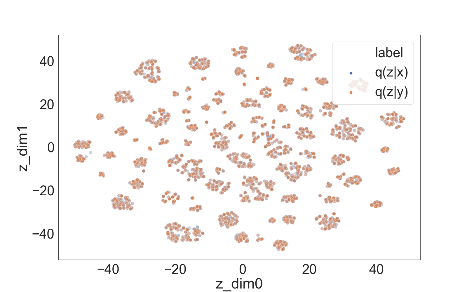
Figure 2: Visualisation of latent variable $z$. Given a pair of $x$ and $y$, $z$ can be sampled from the posterior $q(z|x)$ or $q(z|y)$, denoted by blue and orange dots respectively.

4.4 Analysis

In this section we further analyse the impact of the shared latent variable and also the impact of utilising unlabelled data.

4.4.1 Visualisation of Latent Space

As mentioned in Section 2.1, the latent variable $z$ can be sampled from either posterior approximation $q(z|x)$ or $q(z|y)$. We inspect the latent space in Figure 2 to find out how well the model learns intent sharing. We plot $z$ with the E2E dataset on 2-dimentional space using t-SNE projection Maaten and Hinton (2008).

We observe two interesting properties. First, for each data point ($x$, $y$), the $z$ values sampled from $q(z|x)$ and $q(z|y)$ are close to each other. This reveals that the meanings of $x$ and $y$ are tied in the latent space. Second, there exists distinct clusters in the space of $z$. By further inspecting the actual examples within each cluster, we found that a cluster represents a similar meaning composition. For instance, the cluster centered at (-20, -40) contains {name, foodtype, price, rating, area, near}, while the cluster centered at (45, 10) contains {name, eattype, foodtype, price}. This indicates that the shared latent serves as conclusive global feature representations for NLU and NLG.

4.4.2 Impact of the Latent Variable

One novelty of our model is the introduction of shared latent variable $z$ for natural language $x$ and formal representations $y$. A common problem in neural variational models is that when coupling a powerful autogressive decoder, the decoder tends to learn to ignore $z$ and solely rely on itself to generate the data Bowman et al. (2016); Chen et al. (2017); Goyal et al. (2017). In order to examine to what extent does our model actually rely on the shared variable in both NLU and NLG, we seek for an empirical answer by comparing the $\texttt{JUG}_{\texttt{basic}}$ model with a model variant which uses a random value of $z$ sampled from a normal distribution $N(\mathbf{0},\mathbf{1})$ during testing. From Table 9, we can observe that there exists a large performance drop if $z$ is assigned with random values. This suggests that JUG indeed relies greatly on the shared variable to produce good-quality $x$ or $y$.

Model	NLU	NLG
$\textup{JUG}_{\textup{basic}}$	90.55	0.726
$\textup{JUG}_{\textup{basic}}$ (feed random z)	38.13	0.482

Table 9: A comparative study to evaluate the contribution of the learned latent variable $z$ in NLU/NLG decoding. Models are trained on the whole weather dataset.

Method	NLU			NLG
	Mi	Re	Wr	Mi	Wr
Decoupled	714	256	2382	5714	2317
$\textup{JUG}_{\textup{basic}}$	594	169	1884	4871	2102

Table 10: Error analysis on E2E dataset. Numbers of missing (Mi), redundant (Re) and wrong (Wr) predictions on slot-value pairs are reported for NLU; numbers of missing or wrong generated slot values are listed for NLG. Lower number indicates the better results. Both models are trained on 5% of the training data.

We further analyse the various sources of errors to understand the cases which $z$ helps to improve. On E2E dataset, wrong prediction in NLU comes from either predicting not_mention label for certain slots in ground truth semantics; predicting arbitrary values on slots not present in the ground truth semantics; or predicting wrong values comparing to ground truth. Three types of error are referred to Missing (Mi), Redundant (Re) and Wrong (Wr) in Table 10. For NLG, semantic errors can be either missing or generating wrong slot values in the given semantics Wen et al. (2015). Our model makes fewer mistakes in all these error sources comparing to the baseline Decoupled. We believe this is because the clustering property learned in the latent space provides better feature representations at a global scale, eventually benefiting NLU and NLG.

4.4.3 Impact of Unlabelled Data Source

In Section 4.3, we found that the performance of our model can be further enhanced by leveraging unlabelled data. As we used both unlabelled utterances and unlabelled semantic representations together, it is unclear if both contributed to the performance gain. To answer this question, we start with the $\texttt{JUG}_{\texttt{basic}}$ model, and experimented with adding unlabelled data from 1) only unlabelled utterances $x$; 2) only semantic representations $y$; 3) both $x$ and $y$. As shown in Table 11, when adding any uni-sourced unlabelled data ($x$ or $y$), the model is able to improve to a certain extent. However, the performance can be maximised when both data sources are utilised. This strengthens the argument that our model can leverage bi-sourced unlabelled data more effectively via latent space sharing to improve NLU and NLG at the same time.

	E2E		Weather
Method	NLU	NLG	NLU	NLG
$\textup{JUG}_{\textup{basic}}$	60.30	0.685	73.62	0.634
+unlabelled $x$	62.89	0.765	74.97	0.654
+unlabelled $y$	59.55	0.815	76.98	0.621
+unlabelled $x$ and $y$	68.09	0.814	79.19	0.670

Table 11: Comparison on sources of unlabelled data for semi-supervised learning using only utterances ($x$), only semantic representations ($y$) or both ($x$ and $y$). $\texttt{JUG}_{\texttt{basic}}$ model is trained on 5% of training data.

5 Related Work

Natural Language Understanding (NLU) refers to the general task of mapping natural language to formal representations. One line of research in the dialogue community aims at detecting slot-value pairs expressed in user utterances as a classification problem Henderson et al. (2012); Sun et al. (2014); Mrkšić et al. (2017); Vodolán et al. (2017). Another line of work focuses on converting single-turn user utterances to more structured meaning representations as a semantic parsing task Zettlemoyer and Collins (2005); Jia and Liang (2016); Dong and Lapata (2018); Damonte et al. (2019).

In comparison, Natural Language Generation (NLG) is scoped as the task of generating natural utterances from their formal representations. This is traditionally handled with a pipelined approach Reiter and Dale (1997) with content planning and surface realisation Walker et al. (2001); Stent et al. (2004). More recently, NLG has been formulated as an end-to-end learning problem where text strings are generated with recurrent neural networks conditioning on the formal representation Wen et al. (2015); Dušek and Jurcicek (2016); Dušek et al. (2020); Balakrishnan et al. (2019); Tseng et al. (2019).

There has been very recent work which does NLU and NLG jointly. Both Ye et al. (2019) and Cao et al. (2019) explore the duality of semantic parsing and NLG. The former optimises two sequence-to-sequence models using dual information maximisation, while the latter introduces a dual learning framework for semantic parsing. Su et al. (2019) proposes a learning framework for dual supervised learning Xia et al. (2017) where both NLU and NLG models are optimised towards a joint objective. Their method brings benefits with annotated data in supervised learning, but does not allow semi-supervised learning with unlabelled data. In contrast to their work, we propose a generative model which couples NLU and NLG with a shared latent variable. We focus on exploring a coupled representation space between natural language and corresponding semantic annotations. As proved in experiments, the information sharing helps our model to leverage unlabelled data for semi-supervised learning, which eventually benefits both NLU and NLG.

6 Conclusion

We proposed a generative model which couples natural language and formal representations via a shared latent variable. Since the two space is coupled, we gain the luxury of exploiting each unpaired data source and transfer the acquired knowledge to the shared meaning space. This eventually benefits both NLU and NLG, especially in a low-resource scenario. The proposed model is also suitable for other translation tasks between two modalities.

As a final remark, natural language is richer and more informal. NLU needs to handle ambiguous or erroneous user inputs. However, formal representations utilised by an NLG system are more precisely-defined. In future, we aim to refine our generative model to better emphasise this difference of the two tasks.

Appendix A Appendices

A.1 Derivation of Lower Bounds

We derive the lower bounds for $\log p(x,y)$ as follows:

$$\begin{split}&\log p(x,y)=\log\int_{z}p(x,y,z)\\ &\quad\quad\quad=\log\int_{z}\frac{p(x,y,z)q(z|x)}{q(z|x)}\\ &\quad\quad\quad=\log\int_{z}\frac{p(x|z,y)p(y|z,x)p(z)q(z|x)}{q(z|x)}\\ &\quad\quad\quad=\log\mathbb{E}_{q(z|x)}\frac{p(x|z,y)p(y|z,x)p(z)}{q(z|x)}\\ &\quad\quad\quad\geq\mathbb{E}_{q(z|x)}\log\frac{p(x|z,y)p(y|z,x)p(z)}{q(z|x)}\\ &\quad\quad\quad=\mathbb{E}_{q(z|x)}[\log p(x|z,y)+\log p(y|z,x)]\\ &\quad\quad\quad\quad-\text{KL}[q(z|x)||p(z)]\end{split}$$ (14)

where $q(z|x)$ represents an approximated posterior. This derivation gives us the Equation 6 in the paper. Similarly we can derive an alternative lower bound in Equation 7 by introducing $q(z|y)$ instead of $q(z|x)$.

For marginal log-likelihood $\log p(x)$ or $\log p(y)$, its lower bound is derived as follows:

$$\begin{split}&\log p(x)=\log\int_{y}\int_{z}p(x,y,z)\\ &\quad=\log\int_{y}\int_{z}\frac{p(x|z,y)p(y)p(z)q(z|x)q(y|z,x)}{q(z|x)q(y|z,x)}\\ &\quad=\log\mathbb{E}_{q(y|z,x)}\mathbb{E}_{q(z|x)}\frac{p(x|z,y)p(y)p(z)}{q(z|x)q(y|z,x)}\\ &\quad\geq\mathbb{E}_{q(y|z,x)}\mathbb{E}_{q(z|x)}\log\frac{p(x|z,y)p(y)p(z)}{q(z|x)q(y|z,x)}\\ &\quad=\mathbb{E}_{q(y|z,x)}\mathbb{E}_{q(z|x)}\log p(x|z,y)\\ &\quad\quad-\text{KL}[q(z|x)||p(z)]-\text{KL}[q(y|x,z)||p(y)]\end{split}$$ (15)

Note that the resulting lower bound consists of three terms: a reconstruction of $x$, a KL divergence which regularises the space of $z$, and also a KL divergence which regularises the space of $y$. We have dropped the last term in our optimisation objective in Equation 9, since we do not impose any prior assumption on the output space of the NLU model.

Analogously we can derive the lower bound for $\log p(y)$. We also do not impose any prior assumption on the output space of the NLG model, which leads us to Equation 10.

A.2 Generated Examples

Reference of example

x: "for those prepared to pay over $\pounds$30 , giraffe is a restaurant located near the six bells ."

y: {name=giraffe, eat_type=restaurant, price_range=more than $\pounds$30, near=the six bells}

Prediction by Decoupled model

x: "near the six bells , there is a restaurant called giraffe that is children friendly ." (miss price_range)

y: {name=travellers rest beefeater, price_range=more than $\pounds$30, near=the six bells} (wrong name, miss eat_type)

Prediction by JUG${}_{\textup{semi}}$ model

x: "giraffe is a restaurant near the six bells with a price range of more than $\pounds$30 ." (semantically correct)

y: {name=giraffe, eat_type=restaurant, price_range=more than $\pounds$30, near=the six bells} (exact match)

Table 12: An example of E2E dataset and predictions generated by the baseline model Decoupled and the proposed model $\texttt{JUG}_{\texttt{semi}}$. $x$ and $y$ denotes natural language and the corresponding semantic representation. Errors are highlighted following predictions.

Reference of example
x: "it’s going to be __arg_temp__ and __arg_cloud_coverage__
__arg_colloquial__ between __arg_start_time__ and __arg_end_time__"
y: [__dg_inform__ [__arg_task__ get_forecast ] [__arg_temp__ __arg_temp__ ] [__arg_cloud_coverage__ __arg_cloud_coverage__ ] [__arg_ date_time_range__ [__arg_start_time__ __arg_start_time__ ] [__arg_end_time__ __arg_end_time__ ] [__arg_colloquial__ __arg_colloquial__ ] ] ]
Prediction by Decoupled model
x: "it will be __arg_temp__ degrees and __arg_cloud_coverage__ from
__arg_start_time__ to __arg_end_time__"
y: [__dg_inform__ [__arg_task__ get_forecast ] [__arg_temp__ __arg_temp__ ] [__arg_cloud_coverage__ __arg_cloud_coverage__ ] [__arg_ date_time__ [__arg_colloquial__ __arg_colloquial__ ] ] ] [__dg_inform__ [__arg_task__ get_forecast ] [__arg_temp__ __arg_temp__ ] [__arg_cloud_coverage__ __arg_cloud_coverage__ ] [__arg_date_time_range__ [__arg_start_time__ __arg_start_time__ ] [__arg_end_time__ __arg_end_time__ ] ] ] (not match)
Prediction by JUG_semi model
x: "the temperature will be around __arg_temp__ degrees
__arg_colloquial__ between __arg_start_time__ and __arg_end_time__"
y: [__dg_inform__ [__arg_task__ get_forecast ] [__arg_temp__ __arg_temp__ ] [__arg_cloud_coverage__ __arg_cloud_coverage__ ] [__arg_ date_time_range__ [__arg_start_time__ __arg_start_time__ ] [__arg_end_time__ __arg_end_time__ ] [__arg_colloquial__ __arg_colloquial__ ] ] ] (exact match)

Table 13: An example of weather dataset and predictions generated by the baseline model Decoupled and the proposed model $\texttt{JUG}_{\texttt{semi}}$. $x$ and $y$ denotes natural language and the corresponding semantic representation. NLU result are highlighted following predictions.

References

- Bahdanau et al. (2014) Dzmitry Bahdanau, Kyunghyun Cho, and Yoshua Bengio. 2014. Neural machine translation by jointly learning to align and translate. arXiv preprint arXiv:1409.0473.
- Balakrishnan et al. (2019) Anusha Balakrishnan, Jinfeng Rao, Kartikeya Upasani, Michael White, and Rajen Subba. 2019. Constrained decoding for neural nlg from compositional representations in task-oriented dialogue. arXiv preprint arXiv:1906.07220.
- Banarescu et al. (2013) Laura Banarescu, Claire Bonial, Shu Cai, Madalina Georgescu, Kira Griffitt, Ulf Hermjakob, Kevin Knight, Philipp Koehn, Martha Palmer, and Nathan Schneider. 2013. Abstract meaning representation for sembanking. In Proceedings of the 7th Linguistic Annotation Workshop and Interoperability with Discourse, pages 178–186, Sofia, Bulgaria. Association for Computational Linguistics.
- Berant et al. (2013) Jonathan Berant, Andrew Chou, Roy Frostig, and Percy Liang. 2013. Semantic parsing on Freebase from question-answer pairs. In Proceedings of the 2013 Conference on Empirical Methods in Natural Language Processing, pages 1533–1544, Seattle, Washington, USA. Association for Computational Linguistics.
- Bowman et al. (2016) Samuel R Bowman, Luke Vilnis, Oriol Vinyals, Andrew Dai, Rafal Jozefowicz, and Samy Bengio. 2016. Generating sentences from a continuous space. In Proceedings of The 20th SIGNLL Conference on Computational Natural Language Learning, pages 10–21.
- Cao et al. (2019) Ruisheng Cao, Su Zhu, Chen Liu, Jieyu Li, and Kai Yu. 2019. Semantic parsing with dual learning. ACL.
- Chen et al. (2017) Xi Chen, Diederik P. Kingma, Tim Salimans, Yan Duan, Prafulla Dhariwal, John Schulman, Ilya Sutskever, and Pieter Abbeel. 2017. Variational lossy autoencoder. In 5th International Conference on Learning Representations, ICLR 2017, Toulon, France, April 24-26, 2017, Conference Track Proceedings.
- Damonte et al. (2019) Marco Damonte, Rahul Goel, and Tagyoung Chung. 2019. Practical semantic parsing for spoken language understanding. In Proceedings of the 2019 Conference of the North American Chapter of the Association for Computational Linguistics: Human Language Technologies, Volume 2 (Industry Papers), pages 16–23.
- Dong and Lapata (2018) Li Dong and Mirella Lapata. 2018. Coarse-to-fine decoding for neural semantic parsing. In Proceedings of the 56th Annual Meeting of the Association for Computational Linguistics (Volume 1: Long Papers), pages 731–742.
- Dušek and Jurcicek (2016) Ondřej Dušek and Filip Jurcicek. 2016. Sequence-to-sequence generation for spoken dialogue via deep syntax trees and strings. In Proceedings of the 54th Annual Meeting of the Association for Computational Linguistics (Volume 2: Short Papers), pages 45–51.
- Dušek et al. (2018) Ondřej Dušek, Jekaterina Novikova, and Verena Rieser. 2018. Findings of the e2e nlg challenge. In Proceedings of the 11th International Conference on Natural Language Generation, pages 322–328.
- Dušek et al. (2020) Ondřej Dušek, Jekaterina Novikova, and Verena Rieser. 2020. Evaluating the state-of-the-art of end-to-end natural language generation: The e2e nlg challenge. Computer Speech & Language, 59:123–156.
- Goyal et al. (2017) Anirudh Goyal Alias Parth Goyal, Alessandro Sordoni, Marc-Alexandre Côté, Nan Rosemary Ke, and Yoshua Bengio. 2017. Z-forcing: Training stochastic recurrent networks. In Advances in neural information processing systems, pages 6713–6723.
- He et al. (2016) Di He, Yingce Xia, Tao Qin, Liwei Wang, Nenghai Yu, Tie-Yan Liu, and Wei-Ying Ma. 2016. Dual learning for machine translation. In Proceedings of the 30th International Conference on Neural Information Processing Systems, pages 820–828. Curran Associates Inc.
- Henderson et al. (2012) Matthew Henderson, Milica Gašić, Blaise Thomson, Pirros Tsiakoulis, Kai Yu, and Steve Young. 2012. Discriminative spoken language understanding using word confusion networks. In 2012 IEEE Spoken Language Technology Workshop (SLT), pages 176–181. IEEE.
- Henderson et al. (2014) Matthew Henderson, Blaise Thomson, and Steve Young. 2014. Word-based dialog state tracking with recurrent neural networks. In Proceedings of the 15th Annual Meeting of the Special Interest Group on Discourse and Dialogue (SIGDIAL), pages 292–299.
- Hochreiter and Schmidhuber (1997) Sepp Hochreiter and Jürgen Schmidhuber. 1997. Long short-term memory. Neural computation, 9(8):1735–1780.
- Jia and Liang (2016) Robin Jia and Percy Liang. 2016. Data recombination for neural semantic parsing. In Proceedings of the 54th Annual Meeting of the Association for Computational Linguistics (Volume 1: Long Papers), pages 12–22.
- Juraska et al. (2018) Juraj Juraska, Panagiotis Karagiannis, Kevin Bowden, and Marilyn Walker. 2018. A deep ensemble model with slot alignment for sequence-to-sequence natural language generation. In Proceedings of the 2018 Conference of the North American Chapter of the Association for Computational Linguistics: Human Language Technologies, Volume 1 (Long Papers), pages 152–162.
- Kingma and Ba (2014) Diederik P Kingma and Jimmy Ba. 2014. Adam: A method for stochastic optimization. arXiv preprint arXiv:1412.6980.
- Kingma and Welling (2013) Diederik P Kingma and Max Welling. 2013. Auto-encoding variational bayes. arXiv preprint arXiv:1312.6114.
- Lee (2013) Dong-Hyun Lee. 2013. Pseudo-label: The simple and efficient semi-supervised learning method for deep neural networks. In Workshop on Challenges in Representation Learning, ICML, volume 3, page 2.
- Maaten and Hinton (2008) Laurens van der Maaten and Geoffrey Hinton. 2008. Visualizing data using t-sne. Journal of machine learning research, 9(Nov):2579–2605.
- Mrkšić et al. (2017) Nikola Mrkšić, Diarmuid Ó Séaghdha, Tsung-Hsien Wen, Blaise Thomson, and Steve Young. 2017. Neural belief tracker: Data-driven dialogue state tracking. In Proceedings of the 55th Annual Meeting of the Association for Computational Linguistics (Volume 1: Long Papers), pages 1777–1788.
- Novikova et al. (2017) Jekaterina Novikova, Ondřej Dušek, and Verena Rieser. 2017. The E2E dataset: New challenges for end-to-end generation. In Proceedings of the 18th Annual SIGdial Meeting on Discourse and Dialogue, pages 201–206, Saarbrücken, Germany. Association for Computational Linguistics.
- Pasupat et al. (2019) Panupong Pasupat, Sonal Gupta, Karishma Mandyam, Rushin Shah, Mike Lewis, and Luke Zettlemoyer. 2019. Span-based hierarchical semantic parsing for task-oriented dialog. In Proceedings of the 2019 Conference on Empirical Methods in Natural Language Processing and the 9th International Joint Conference on Natural Language Processing (EMNLP-IJCNLP), pages 1520–1526, Hong Kong, China. Association for Computational Linguistics.
- Reiter and Dale (1997) Ehud Reiter and Robert Dale. 1997. Building applied natural language generation systems. Natural Language Engineering, 3(1):57–87.
- Sennrich et al. (2016) Rico Sennrich, Barry Haddow, and Alexandra Birch. 2016. Improving neural machine translation models with monolingual data. In Proceedings of the 54th Annual Meeting of the Association for Computational Linguistics (Volume 1: Long Papers), pages 86–96.
- Stent et al. (2004) Amanda Stent, Rashmi Prasad, and Marilyn Walker. 2004. Trainable sentence planning for complex information presentation in spoken dialog systems. In Proceedings of the 42nd annual meeting on association for computational linguistics, page 79. Association for Computational Linguistics.
- Su et al. (2019) Shang-Yu Su, Chao-Wei Huang, and Yun-Nung Chen. 2019. Dual supervised learning for natural language understanding and generation. ACL.
- Sun et al. (2014) Kai Sun, Lu Chen, Su Zhu, and Kai Yu. 2014. The sjtu system for dialog state tracking challenge 2. In Proceedings of the 15th Annual Meeting of the Special Interest Group on Discourse and Dialogue (SIGDIAL), pages 318–326.
- Tseng et al. (2019) Bo-Hsiang Tseng, Paweł Budzianowski, Yen-chen Wu, and Milica Gasic. 2019. Tree-structured semantic encoder with knowledge sharing for domain adaptation in natural language generation. In Proceedings of the 20th Annual SIGdial Meeting on Discourse and Dialogue, pages 155–164.
- Vodolán et al. (2017) Miroslav Vodolán, Rudolf Kadlec, Jan Kleindienst, and V Parku. 2017. Hybrid dialog state tracker with asr features. EACL 2017, page 205.
- Walker et al. (2001) Marilyn A Walker, Owen Rambow, and Monica Rogati. 2001. Spot: A trainable sentence planner. In Proceedings of the second meeting of the North American Chapter of the Association for Computational Linguistics on Language technologies, pages 1–8. Association for Computational Linguistics.
- Wen et al. (2015) Tsung-Hsien Wen, Milica Gasic, Nikola Mrkšić, Pei-Hao Su, David Vandyke, and Steve Young. 2015. Semantically conditioned lstm-based natural language generation for spoken dialogue systems. In Proceedings of the 2015 Conference on Empirical Methods in Natural Language Processing, pages 1711–1721.
- Williams (1992) Ronald J Williams. 1992. Simple statistical gradient-following algorithms for connectionist reinforcement learning. Machine learning, 8(3-4):229–256.
- Xia et al. (2017) Yingce Xia, Tao Qin, Wei Chen, Jiang Bian, Nenghai Yu, and Tie-Yan Liu. 2017. Dual supervised learning. In Proceedings of the 34th International Conference on Machine Learning-Volume 70, pages 3789–3798. JMLR. org.
- Ye et al. (2019) Hai Ye, Wenjie Li, and Lu Wang. 2019. Jointly learning semantic parser and natural language generator via dual information maximization. arXiv preprint arXiv:1906.00575.
- Young et al. (2010) Steve Young, Milica Gašić, Simon Keizer, François Mairesse, Jost Schatzmann, Blaise Thomson, and Kai Yu. 2010. The hidden information state model: A practical framework for pomdp-based spoken dialogue management. Computer Speech & Language, 24(2):150 – 174.
- Yu et al. (2018) Tao Yu, Zifan Li, Zilin Zhang, Rui Zhang, and Dragomir Radev. 2018. Typesql: Knowledge-based type-aware neural text-to-sql generation. In Proceedings of the 2018 Conference of the North American Chapter of the Association for Computational Linguistics: Human Language Technologies, Volume 2, pages 588–594.
- Zettlemoyer and Collins (2005) Luke S Zettlemoyer and Michael Collins. 2005. Learning to map sentences to logical form: structured classification with probabilistic categorial grammars. In Proceedings of the Twenty-First Conference on Uncertainty in Artificial Intelligence, pages 658–666. AUAI Press.
- Zettlemoyer and Collins (2012) Luke S Zettlemoyer and Michael Collins. 2012. Learning to map sentences to logical form: Structured classification with probabilistic categorial grammars. arXiv preprint arXiv:1207.1420.
- Zhang and Wang (2016) Xiaodong Zhang and Houfeng Wang. 2016. A joint model of intent determination and slot filling for spoken language understanding. In Proceedings of the Twenty-Fifth International Joint Conference on Artificial Intelligence, pages 2993–2999. AAAI Press.