Asymptotic preserving IMEX-DG-S schemes for linear kinetic transport equations based on Schur complement

Abstract

We consider a linear kinetic transport equation under a diffusive scaling, that converges to a diffusion equation as the Knudsen number $\varepsilon\rightarrow 0$. In [3, 21], to achieve the asymptotic preserving (AP) property and unconditional stability in the diffusive regime with $\varepsilon\ll 1$, numerical schemes are developed based on an additional reformulation of the even-odd or micro-macro decomposed version of the equation. The key of the reformulation is to add a weighted diffusive term on both sides of one equation in the decomposed system. The choice of the weight function, however, is problem-dependent and ad-hoc, and it can affect the performance of numerical simulations. To avoid issues related to the choice of the weight function and still obtain the AP property and unconditional stability in the diffusive regime, we propose in this paper a new family of AP schemes, termed as IMEX-DG-S schemes, directly solving the micro-macro decomposed system without any further reformulation. The main ingredients of the IMEX-DG-S schemes include globally stiffly accurate implicit-explicit (IMEX) Runge-Kutta (RK) temporal discretizations with a new IMEX strategy, discontinuous Galerkin (DG) spatial discretizations, discrete ordinate methods for the velocity space, and the application of the Schur complement to the algebraic form of the schemes to control the overall computational cost. The AP property of the schemes is shown formally. With an energy type stability analysis applied to the first order scheme, and Fourier type stability analysis applied to the first to third order schemes, we confirm the uniform stability of the methods with respect to $\varepsilon$ and the unconditional stability in the diffusive regime. A series of numerical examples are presented to demonstrate the performance of the new schemes.

1 Introduction

Important physical phenomena like radiative transfer and neutron transport can be modeled by kinetic transport equations. In this work, we consider a linear kinetic transport equation under a diffusive scaling:

$$\varepsilon\partial_{t}f+v\partial_{x}f=\frac{\sigma_{s}}{\varepsilon}(\langle f\rangle-f)-\varepsilon\sigma_{a}f.$$ (1.1)

Here, $f(x,v,t)$ is the probability distribution function of particles, $x\in\Omega_{x}$ is the spatial position, $v\in\Omega_{v}$ is the velocity with $\Omega_{v}$ being bounded, and $t$ is time. $\sigma_{s}(x)\geq 0$ and $\sigma_{a}(x)\geq 0$ are the scattering and the absorption coefficients, respectively. $\langle f\rangle=\int_{\Omega_{v}}fd\nu$, where $\nu$ is a measure of the velocity space satisfying $\int_{\Omega_{v}}d\nu=1$. $\varepsilon>0$ denotes the Knudsen number, which is the ratio of mean free path of particles to the characteristic length.

The linear kinetic transport equation (1.1) has a multiscale nature. With the assumption $\sigma_{s}>0$, the kinetic transport equation will converge to its diffusion limit as $\varepsilon\rightarrow 0$:

$$\partial_{t}\rho=\langle v^{2}\rangle\partial_{x}(\partial_{x}\rho/\sigma_{s})-\sigma_{a}\rho,$$ (1.2)

where $\rho=\langle f\rangle$ is the macroscopic density of particles. This multiscale nature poses computational challenges: (1) a standard explicit numerical scheme has a time step restriction $\Delta t\leq O(\varepsilon h)$ ($h$ is the mesh size) due to numerical stability, with prohibitive computational cost for small $\varepsilon$; (2) an implicit scheme, though possibly being unconditionally stable and hence not suffering from stability issue, may still fail to capture the correct physical limit as $\varepsilon\rightarrow 0$ on under-resolved meshes [4, 20].

Asymptotic preserving (AP) schemes [11, 8], which preserve the asymptotic behavior of the physical model on the discrete level, are a well established candidate to address above challenges. An AP scheme for (1.1) converges to a scheme solving the limiting diffusion equation (1.2) as $\varepsilon\rightarrow 0$, while being consistent and stable for a broad range of $\varepsilon$, even on under-resolved meshes for small $\varepsilon$. AP schemes having explicit limiting schemes are considered in [12, 14, 13, 16, 10]. With the diffusive nature of the physical limit and the explicitness of the limiting schemes, these methods have a parabolic time step restriction $\Delta t=O(h^{2})$ in the diffusive regime $\varepsilon\ll 1$. To enhance the stability, AP schemes with implicit limiting schemes are developed in [3, 21], and they are demonstrated, either numerically or analytically, to be unconditionally stable in the diffusive regime.

To achieve unconditional stability in the diffusive regime, in [3], a second reformulation is introduced to the even-odd decomposition [17, 13] of (1.1). And a similar strategy is applied to the micro-macro decomposition [19] of (1.1) in [21]. Taking the methods in [21] as an example, a weighted diffusive term $\omega\partial_{x}(\partial_{x}\rho/\sigma_{s})$, determined by the diffusion limit, is added to both sides of one equation in the micro-macro decomposed system. Then, a suitable implicit-explicit (IMEX) Runge-Kutta (RK) time discretization is applied to the newly reformulated system. Under the adopted IMEX strategy, the two added diffusive terms are treated differently. In space, local discontinuous Galerkin (LDG) method [7] is applied. The resulting IMEX-LDG schemes are AP and can be high order, with the limiting schemes being implicit to solve the diffusion limit. Based on Fourier analysis, stability condition is obtained in [21] by numerically solving an eigenvalue problem, and it confirms the unconditional stability in the diffusive regime. Following an energy approach, the stability condition is rigorously established in [22] for the first order in time scheme applied to the model with general material properties $\sigma_{s}(x)$ and $\sigma_{a}(x)$.

In a multiscale problem, $\sigma_{s}(x)$ may vary spatially, and the diffusion dominant and transport dominant subregions can coexist. Despite the success of enhancing the stability in the diffusive regime, the strategy in [3, 21] with an additional reformulation also faces some issues. First, the choice of the numerical weight is problem-dependent, and this ad-hoc choice has an influence on the performance of numerical simulations. Second, when the scattering coefficient $\sigma_{s}(x)$ varies spatially, intuitively, a spatially dependent weight function $\omega$ seems to be preferred to better capture the multiscale behavior. However, with such a spatially dependent weight, an extra non-physical assumption would be needed to maintain local conservation property, see Section 2 for more discussions.

To overcome these issues and still accomplish unconditional stability in the diffusive regeime, we here design a new family of IMEX discontinuous Galerkin (DG) AP schemes based on the Schur complement [25], referred to as IMEX-DG-S methods. Our new schemes directly solve the micro-macro decomposed system without any additional reformulation, and hence they do not suffer from issues mentioned above. In time, we apply globally stiffly accurate IMEX-RK time integrators [3] with a new IMEX strategy. In space, we use DG discretizations [6] with carefully chosen numerical fluxes. In the velocity space, a discrete ordinates method [23] is utilized. On the solver level, the key is to apply the Schur complement to the fully discrete system, and this is important for the computational cost. Indeed our proposed methods have comparable computational complexity as the IMEX-LDG schemes in [21]. As $\varepsilon\rightarrow 0$, asymptotic analysis shows that our new schemes formally converge to high order methods that involve implicit RK methods in time and LDG methods in space solving the diffusion limit, implying the AP property of the schemes. When an initial layer exists in the solution, our schemes no longer need special treatment for the first step as in [21] in order to stay AP. With an energy type stability analysis applied to the first order scheme, and Fourier type stability analysis applied to the first to third order schemes, we obtain stability conditions that confirm the uniform stability of the methods with respect to $\varepsilon$ and the unconditional stability in the diffusive regime. A discrete energy different from that in [9, 22] is used in the energy analysis. Numerical examples are presented to demonstrate the performance of the IMEX-DG-S schemes and its advantage over the IMEX-LDG schemes in some test cases.

The rest of the paper is organized as follows. In Section 2, we present the micro-macro decomposition, and briefly review the additional reformulation strategy in [21] to motivate our work. In Section 3, we define our numerical schemes, and provide the details of the Schur complement for the final matrix-vector system. In Section 4, formal asymptotic analysis is presented to confirm the AP property. In Section 5, energy and Fourier analyses are performed to obtain stability conditions. In Section 6, numerical results are reported to illustrate the performance of the proposed schemes, and this will be followed by conclusions in Section 7.

2 Micro-macro decomposition and motivation

Following the micro-macro decomposition framework [19, 16], we reformulate (1.1). We first define a scattering operator $\mathcal{L}f=\langle f\rangle-f$, and let $\Pi$ denote the $L^{2}$ projection onto the null space of $\mathcal{L}$: $\textrm{Null}(\mathcal{L})=\textrm{Span}\{1\}$. We then decompose $f$ orthogonally into $f=\rho+\varepsilon g$, where $\rho:=\Pi f=\langle f\rangle$, and $g:=\frac{1}{\varepsilon}({\bf{I}}-\Pi)f$ satisfying $\langle g\rangle=0$. Finally we apply $\Pi$ and its orthogonal complement ${\bf{I}}-\Pi$ to (1.1), and obtain the micro-macro decomposed system:

$$\partial_{t}\rho+\partial_{x}\langle vg\rangle=-\sigma_{a}\rho,$$ (2.1a)

$$\varepsilon \partial_{t}g+({\bf{I}}-\Pi)\partial_{x}(vg)+\frac{1}{\varepsilon}v\partial_{x}\rho=-\frac{\sigma_{s}}{\varepsilon}g-\varepsilon\sigma_{a}g.$$ (2.1b)

Assume $\sigma_{s}(x)>0$. As the Knudsen number $\varepsilon\rightarrow 0$, (2.1) formally converges to its diffusion limit

$$\sigma_{s}g=-v\partial_{x}\rho,\qquad\partial_{t}\rho=-\partial_{x}\langle vg\rangle-\sigma_{a}\rho=\langle v^{2}\rangle\partial_{x}(\partial_{x}\rho/\sigma_{s})-\sigma_{a}\rho.$$ (2.2)

To define AP schemes with unconditional stability in the diffusive regime with $\varepsilon\ll 1$, [21] applies a second reformulation to (2.1) by adding the weighted diffusive term $\langle v^{2}\rangle\partial_{x}(\omega\partial_{x}\rho/\sigma_{s})$ to both sides of (2.1a):

$$\partial_{t}\rho+\partial_{x}\langle v\left(g+v\omega(\partial_{x}\rho/\sigma_{s})\;\right)\rangle=\langle v^{2}\rangle\partial_{x}(\omega\partial_{x}\rho/\sigma_{s})-\sigma_{a}\rho,$$ (2.3a)

$$\varepsilon \partial_{t}g+({\bf{I}}-\Pi)\partial_{x}(vg)+\frac{1}{\varepsilon}v\partial_{x}\rho=-\frac{\sigma_{s}}{\varepsilon}g-\varepsilon\sigma_{a}g.$$ (2.3b)

Here, $\omega$ is a non-negative numerical weight function, and it satisfies $\omega\rightarrow 1$ as $\varepsilon\rightarrow 0$.

In [21], globally stiffly accurate IMEX-RK time discretizations are applied, where the weighted diffusive term $\langle v^{2}\rangle\partial_{x}(\omega\partial_{x}\rho/\sigma_{s})$ on the left hand side of (2.3a) is treated explicitly and that on the right hand side is treated implicitly. With LDG methods further applied in space, the resulting schemes are AP, unconditionally stable in the diffusive regime, and they also show good performance numerically. However, the choice of $\omega$ is problem-dependent, and it can affect the performance of the methods (see. e.g. Examples 2, 4, 5 in Section 6). Moreover, when $\sigma_{s}(x)$ is not constant, a spatially dependent weight $\omega$ would be preferred intuitively in order to better capture the multiscale behavior. If such weight function is used, one would need to assume $\omega\partial_{x}\rho/\sigma_{s}$ to be continuous to ensure the local conservation, and this is apparently not physical due to the weight-dependence. As far as we know, only weight functions that do not vary spatially have been considered in the literature.

3 Numerical methods

In this section, we will design a new family of AP schemes directly based on the micro-macro decomposition (2.1), aiming at achieving unconditional stability in the diffusive regime without the need for a weight function. In the following subsections, we will present discretizations in time, in space, and in velocity. For the fully discrete schemes, Schur complement will be applied to their algebraic systems. We end this section by extending the IMEX strategy to some more general kinetic transport models. Throughout this section, periodic boundary conditions are assumed in space.

3.1 Time discretization

In time, we apply globally stiffly accurate IMEX-RK methods of type ARS. The first order one is defined as follows. Given $\rho^{n}$ and $g^{n}$ at $t=t^{n}$, we seek $\rho^{n+1}$ and $g^{n+1}$ at $t^{n+1}=t^{n}+\Delta t$, which satisfy

$$\frac{\rho^{n+1}-\rho^{n}}{\Delta t}+\partial_{x}\langle vg^{n+1}\rangle=-\sigma_{a}\rho^{n+1},$$ (3.1a)

$$\frac{g^{n+1}-g^{n}}{\Delta t}+\frac{1}{\varepsilon}({\bf{I}}-\Pi)(v\partial_{x}g^{n})+\frac{1}{\varepsilon^{2}}v\partial_{x}\rho^{n+1}=-\frac{1}{\varepsilon^{2}}\sigma_{s}g^{n+1}-\sigma_{a}g^{n+1}.$$ (3.1b)

The same IMEX strategy in (3.1) will be also used to achieve high order temporal accuracy. Recall that a general IMEX-RK scheme can be represented by a double Butcher tableau:

$$\begin{array}[]{c|c}\tilde{c}&\tilde{\mathcal{A}}\\ \hline\cr&{\tilde{b}}^{T}\end{array}\ \ \ \ \ \begin{array}[]{c|c}{c}&{\mathcal{A}}\\ \hline\cr&{b^{T}}\end{array}~{}~{}.$$ (3.2)

Here, $\tilde{\mathcal{A}}=(\tilde{a}_{ij})$, $\mathcal{A}=(a_{ij})$ are $s\times s$ lower triangular matrices, and $\tilde{a}_{ii}=0$, $i=1,\cdots s$. $\tilde{b}=(\tilde{b}_{i})$, $b=(b_{i})$, $\tilde{c}=(\tilde{c}_{i}),$ and $c=(c_{i})$ are $s$-dimensional vectors, and $\tilde{c}_{i}=\sum_{j=1}^{i-1}\tilde{a}_{ij}$, $c_{i}=\sum_{j=1}^{i}a_{ij}$. An IMEX-RK scheme is globally stiffly accurate [3] if

$$c_{s}=\tilde{c}_{s}=1,\;\text{and}\;b_{j}=a_{sj},\;\tilde{b}_{j}=\tilde{a}_{sj},\;\forall j=1,\dots,s,$$

and it is of type ARS [1] if

$$\mathcal{A}=\left[\begin{array}[]{cc}0&0\\ 0&\hat{\mathcal{A}}\end{array}\right],\quad\textrm{where}\;\hat{\mathcal{A}}\;\textrm{is invertible}.$$ (3.3)

For the second and third order accuracy, we use ARS(2,2,2) and ARS(4,4,3), respectively [1, 3].

3.2 Space discretization

Let $\Omega_{x}=[x_{L},x_{R}]$ be the computational domain, and $\Omega_{h}=\left\{I_{i}=[x_{i-\frac{1}{2}},x_{i+\frac{1}{2}}],i=1,\dots,N\right\}$ be a partition of $\Omega_{x}$. Let $x_{i}=({x_{i-\frac{1}{2}}+x_{i+\frac{1}{2}}})/{2}$, $h_{i}=x_{i+\frac{1}{2}}-x_{i-\frac{1}{2}}$, $h=\max_{i}{h_{i}}$. Given a nonnegative integer $k$, define the discrete space $U_{h}^{k}=\{u\in L^{2}(\Omega_{x}):u|_{I_{i}}\in P^{k}(I_{i}),\forall 1\leq i\leq N\}$, where $P^{k}(I_{i})$ denotes the space of polynomials with degree at most $k$ on $I_{i}$. Define $u^{\pm}_{i+\frac{1}{2}}=\lim_{\Delta x\rightarrow 0^{\pm}}u(x_{i+\frac{1}{2}}+\Delta x)$ and the jump $[u]_{i+\frac{1}{2}}=u^{+}_{i+\frac{1}{2}}-u^{-}_{i-\frac{1}{2}}$, $\forall i$.

We apply the following DG spatial discretization to the semi-discrete method in (3.1). Given numerical solutions $\rho_{h}^{n}$ and $g_{h}^{n}\in U_{h}^{k}$, we look for $\rho_{h}^{n+1},g_{h}^{n+1}\in U_{h}^{k}$ satisfying, $\forall{\phi},{\psi}\in U_{h}^{k}$

$$(\frac{\rho_{h}^{n+1}-\rho_{h}^{n}}{\Delta t},{\phi})+l_{h}\left(\langle vg_{h}^{n+1}\rangle,{\phi}\right)=-\left(\sigma_{a}\rho_{h}^{n+1},{\phi}\right),$$ (3.4a)

$$(\frac{g_{h}^{n+1}-g_{h}^{n}}{\Delta t},{\psi})+\frac{1}{\varepsilon}\widetilde{b}_{h,v}(g_{h}^{n},{\psi})-\frac{1}{\varepsilon^{2}}vd_{h}(\rho_{h}^{n+1},{\psi})=-\frac{1}{\varepsilon^{2}}(\sigma_{s}g_{h}^{n+1},{\psi})-(\sigma_{a}g_{h}^{n+1},{\psi}).$$ (3.4b)

Here, $(\cdot,\cdot)$ is the standard $L^{2}$ inner product of $L^{2}(\Omega_{x})$. Bilinear forms $d_{h}(\cdot,\cdot)$, $l_{h}(\cdot,\cdot)$, $\widetilde{b}_{h,v}(\cdot,\cdot)$ are defined as

$$d_{h}(\rho_{h},{\psi}) =\sum_{i}\int_{I_{i}}\rho_{h}\partial_{x}{\psi}dx+\sum_{i}(\breve{\rho_{h}})_{{i-\frac{1}{2}}}[{\psi}]_{i-\frac{1}{2}},$$ (3.5a)

$$l_{h}(\langle vg_{h}\rangle,{\phi}) =-\sum_{i}\int_{I_{i}}\langle vg_{h}\rangle\partial_{x}{\phi}dx-\sum_{i}\widehat{\langle vg_{h}\rangle}_{i-\frac{1}{2}}[{\phi}]_{i-\frac{1}{2}},$$ (3.5b)

$$\widetilde{b}_{h,v}(g_{h},{\psi}) =(({\bf{I}}-\Pi){\mathcal{D}}^{up}_{h}(g_{h};v),{\psi})=({\mathcal{D}}^{up}_{h}(g_{h};v)-\langle{\mathcal{D}}^{up}_{h}(g_{h};v)\rangle,{\psi}),$$ (3.5c)

where ${\mathcal{D}}^{up}_{h}(g_{h};v)\in U_{h}^{k}$ is an upwind approximation to $v\partial_{x}g$ for any given velocity $v$:

$$({\mathcal{D}}^{up}_{h}(g_{h};v),{\psi})=-\sum_{i}\left(\int_{I_{i}}vg_{h}\partial_{x}{\psi}dx\right)-\sum_{i}\widetilde{(vg_{h})}_{i-\frac{1}{2}}[{\psi}]_{i-\frac{1}{2}},\quad\forall\psi\in U_{h}^{k}.$$ (3.6)

$(\widetilde{vg_{h}})_{i-\frac{1}{2}}$, $\widehat{\langle vg_{h}\rangle}_{i-\frac{1}{2}}$ and $(\breve{\rho_{h}})_{i-\frac{1}{2}}$ are numerical fluxes and chosen as:

$$\textrm{upwind:}\quad(\widetilde{vg_{h}})_{i-\frac{1}{2}}:=\left\{\begin{array}[]{ll}({vg_{h}})_{i-\frac{1}{2}}^{-},&\mbox{if}\;v\geq 0,\\ ({vg_{h}})_{i-\frac{1}{2}}^{+},&\mbox{if}\;v<0,\end{array}\right.\;\;$$ (3.7c)

$$\textrm{alternating:}\quad(\breve{\rho_{h}})_{i-\frac{1}{2}}=(\rho_{h})_{i-\frac{1}{2}}^{-},\;\;\widehat{\langle vg_{h}\rangle}_{i-\frac{1}{2}}={\langle vg_{h}\rangle}_{i-\frac{1}{2}}^{+}.$$ (3.7d)

Based on the Riesz representation, we can further find two well-defined bounded linear operators ${\mathcal{D}}_{h}^{-},{\mathcal{D}}_{h}^{+}:U_{h}^{k}\rightarrow U_{h}^{k}$ such that

$$({\mathcal{D}}_{h}^{-}{\phi},{\psi})=-d_{h}({\phi},{\psi}),\;\;({\mathcal{D}}_{h}^{+}{\phi},{\psi})=l_{h}({\phi},{\psi}),\;\;\forall{\phi},{\psi}\in U_{h}^{k}.$$

${\mathcal{D}}_{h}^{\pm}$ can be seen as discrete derivative operators, and the scheme (3.4) can be rewritten as:

$$\frac{\rho_{h}^{n+1}-\rho_{h}^{n}}{\Delta t}+{\mathcal{D}}_{h}^{+}\langle vg_{h}^{n+1}\rangle=-\pi_{h}(\sigma_{a}\rho_{h}^{n+1}),$$ (3.8a)

$$\frac{g_{h}^{n+1}-g_{h}^{n}}{\Delta t}+\frac{1}{\varepsilon}({\bf{I}}-\Pi){\mathcal{D}}^{up}_{h}(g^{n}_{h};v)+\frac{v}{\varepsilon^{2}}{\mathcal{D}}_{h}^{-}\rho_{h}^{n+1}=-\frac{1}{\varepsilon^{2}}\pi_{h}(\sigma_{s}g_{h}^{n+1})-\pi_{h}(\sigma_{a}g_{h}^{n+1}),.$$ (3.8b)

with $\pi_{h}$ being the $L^{2}$ projection onto $U_{h}^{k}$.

The DG spatial discretization can be coupled directly with high order IMEX-RK time integrators. At $t=0$, $\rho_{h}^{0}$ and $g_{h}^{0}$ are initialized by $L^{2}$ projection, namely, $\rho_{h}^{0}=\pi_{h}(\rho(x,0))$ and $g_{h}^{0}=\pi_{h}(g(x,v,0))$. The following lemma summarizes a property of the bilinear forms $l_{h}$ and $d_{h}$, and it is important in stability analysis and can be easily verified.

Lemma 3.1.

With periodic boundary conditions in space, there hold

$$l_{h}({\phi},{\psi})=d_{h}({\psi},{\phi}),\;\;\forall{\phi},{\psi}\in U_{h}^{k},\quad\text{and}\quad{\mathcal{D}}_{h}^{+}=-({\mathcal{D}}_{h}^{-})^{\top},$$ (3.9)

where the superscript ^⊤ to an operator denotes its adjoint.

3.3 Velocity discretization

In velocity variable, we will apply the discrete ordinates method [23]. Let $\{v_{l}\}_{l=1}^{N_{v}}$ denote a set of quadrature points as collocation points in the velocity space $\Omega_{v}$ and $\{\omega_{l}\}_{l=1}^{N_{v}}$ be the corresponding quadrature weights. An integral in velocity will be approximated by

$$\langle\eta(v)\rangle=\int_{\Omega_{v}}\eta(v)d\nu\approx\sum_{l=1}^{N_{v}}\omega_{l}\eta(v_{l})\triangleq:\langle\eta(v)\rangle_{h},\;$$ (3.10)

Particularly, we choose $\{\omega_{l}\}_{l=1}^{N_{v}}$ and $\{v_{l}\}_{l=1}^{N_{v}}$ satisfying

$$\langle v^{2}\rangle=\langle v^{2}\rangle_{h}.$$ (3.11)

This requirement is essential for our fully discrete schemes to capture the correct diffusion limit as $\varepsilon\rightarrow 0$.

3.4 Fully discrete schemes

By combining the temporal, spatial, and velocity discretizations described above, we are now ready to present the fully discrete schemes: Given $\rho_{h}^{n}\in U_{h}^{k}$, $\{g_{h,l}^{n}\}_{l=1}^{N_{v}}\in U_{h}^{k}$, we look for $\rho_{h}^{n+1}\in U_{h}^{k}$, $\{g_{h,l}^{n+1}\}_{l=1}^{N_{v}}\in U_{h}^{k}$, satisfying for $i=1,\dots,s$, $l=1,\dots,N_{v}$

$$(\rho_{h}^{n,(i)},{\phi}) =(\rho_{h}^{n},{\phi})-\Delta t\sum_{j=1}^{i}a_{ij}\left(({\mathcal{D}}_{h}^{+}\langle vg_{h}^{n,(j)}\rangle_{h},{\phi})+(\sigma_{a}\rho_{h}^{n,(j)},{\phi})\right),\forall{\phi}\in U_{h}^{k}$$ (3.12a)

$$\varepsilon^{2}(g_{h,l}^{n,(i)},{\psi}) =\varepsilon^{2}(g_{h,l}^{n},{\psi})-\varepsilon\Delta t\sum_{j=1}^{i-1}\tilde{a}_{ij}\left(({\mathcal{D}}^{up}_{h}(g^{n,(j)}_{h};v_{l}),{\psi})-(\langle{\mathcal{D}}^{up}_{h}(g^{n,(j)}_{h};v)\rangle_{h},{\psi})\right)$$

$$- \Delta t\sum_{j=1}^{i}a_{ij}\left(v_{l}({\mathcal{D}}_{h}^{-}\rho_{h}^{n,(j)},{\psi})+(\sigma_{s}g_{h,l}^{n,(j)},{\psi})+\varepsilon^{2}(\sigma_{a}g_{h,l}^{n,(j)},{\psi})\right),\forall{\psi}\in U_{h}^{k}$$ (3.12b)

$$\rho_{h}^{n+1} =\rho_{h}^{n,(s)},\quad g_{h,l}^{n+1}=g_{h,l}^{n,(s)}.$$ (3.12c)

We here have used $g_{h,l}^{n}:=g_{h}^{n}(\cdot,v_{l})$, $g_{h,l}^{n,(i)}:=g_{h}^{n,(i)}(\cdot,v_{l})$, and $\langle\mathcal{G}(g_{h}^{n,(j)})\rangle_{h}=\sum_{l=1}^{N_{v}}\omega_{l}\mathcal{G}(g_{h,l}^{n,(j)})$ with $\mathcal{G}:L^{2}(\Omega_{v})\rightarrow L^{2}(\Omega_{v})$. And the intermediate functions $\rho_{h}^{n,(i)},g_{h,l}^{n,(i)}$ are also in $U_{h}^{k}$.

Particularly, the first order in time scheme is: $\forall{\phi},{\psi}\in U_{h}^{k}$, $l=1,\dots,N_{v}$,

$$(\frac{\rho_{h}^{n+1}-\rho_{h}^{n}}{\Delta t},{\phi})+l_{h}\left(\langle vg_{h}^{n+1}\rangle_{h},{\phi}\right)=-\left(\sigma_{a}\rho_{h}^{n+1},{\phi}\right),$$ (3.13a)

$$(\frac{g_{h,l}^{n+1}-g_{h,l}^{n}}{\Delta t},{\psi})+\frac{1}{\varepsilon}b_{h,v}(g_{h,l}^{n},{\psi})-\frac{1}{\varepsilon^{2}}vd_{h}(\rho_{h}^{n+1},{\psi})=-\frac{1}{\varepsilon^{2}}(\sigma_{s}g_{h,l}^{n+1},{\psi})-(\sigma_{a}g_{h,l}^{n+1},{\psi}),$$ (3.13b)

where

$$b_{h,v}(g_{h,l}^{n},{\psi})=({\mathcal{D}}^{up}_{h}(g^{n}_{h};v_{l}),{\psi})-(\langle{\mathcal{D}}^{up}_{h}(g^{n}_{h};v)\rangle_{h},{\psi}).$$ (3.14)

From here on, we will use IMEX$p$-DG-S to refer to the fully discrete scheme with $p$-th order IMEX-RK time integrator, and use IMEX$p$-DG$k$-S with the discrete space $U_{h}^{k-1}$ in the spatial discretization. Here S stands for the Schur complement, which will be discussed in next subsection. Finally one can obtain the following property of the numerical solution following a similar proof of Lemma 3.1 in [9],

$$\langle g_{h}^{n}\rangle_{h}=0,\quad\forall n\geq 0.$$ (3.15)

3.5 Matrix-vector formulation and Schur complement

To implement the proposed schemes, we will further apply Schur complement at the algebraic level. With this, our methods will have comparable computational complexity as the IMEX-LDG schemes in [21, 22]. Next we use the first order in time IMEX1-DG-S scheme to illustrate. Similar discussion can go to the high order in time schemes.

We start with the matrix-vector formulation of the IMEX1-DG-S scheme (3.13). Let $\{e_{l}(x)\}_{l=1}^{m}$ be a basis of the discrete space $U_{h}^{k}$. Define ${\bf{e}}=(e_{1}(x),\dots,e_{m}(x))^{T}$. Then the numerical solutions can be expanded as

$$\rho_{h}^{n}(x)=\sum_{i=1}^{m}\rho_{i}^{n}e_{i}(x)=({\boldsymbol{\rho}}^{n})^{T}{\bf{e}},\;\;g_{h,j}^{n}(x)=\sum_{i=1}^{m}g^{n}_{j,i}e_{i}(x)=({\bf{g}}^{n}_{j})^{T}{\bf{e}},$$

where ${\boldsymbol{\rho}}^{n}=(\rho_{1}^{n},\dots,\rho_{m}^{n})^{T}$ and ${\bf{g}}^{n}_{j}=(g_{j,1}^{n},\dots,g_{j,m}^{n})^{T}$.

Define the mass matrix $(M)_{ij}=(e_{j},e_{i})$ and stiff matrices $(D^{+})_{ij}=({\mathcal{D}}_{h}^{+}e_{j},e_{i})$, $(D^{-})_{ij}=({\mathcal{D}}_{h}^{-}e_{j},e_{i})$. Also define $(\Sigma_{s})_{ij}=(\sigma_{s}e_{j},e_{i})$ and $(\Sigma_{a})_{ij}=(\sigma_{a}e_{j},e_{i})$. The fully discrete IMEX1-DG-S scheme (3.13) can be written into its matrix-vector form:

$$\mathcal{L}\left({\boldsymbol{\rho}}^{n+1},{\bf{g}}_{1}^{n+1},{\bf{g}}_{2}^{n+1},\dots\bf{g}_{N_{v}}^{n+1}\right)^{T}=\left({\bf{b}}_{0}^{n},{\bf{b}}_{1}^{n},{\bf{b}}_{2}^{n},\dots,{\bf{b}}_{N_{v}}^{n}\right)^{T},\quad\text{and,}$$ (3.16a)

$$\mathcal{L}=\left(\begin{matrix}M+\Delta t\Sigma_{a}&\Delta t\omega_{1}v_{1}D^{+}&\Delta t\omega_{2}v_{2}D^{+}&\dots&\Delta t\omega_{N_{v}}v_{N_{v}}D^{+}\\ v_{1}\Delta tD^{-}&\Theta&0&\dots&0\\ v_{2}\Delta tD^{-}&0&\Theta&\dots&0\\ \vdots&\vdots&\vdots&\ddots&\vdots\\ v_{N_{v}}\Delta tD^{-}&0&0&\dots&\Theta\end{matrix}\right).$$ (3.16b)

Here $\Theta=\varepsilon^{2}(M+\Delta t\Sigma_{a})+\Delta t\Sigma_{s}$, and ${\bf{b}}_{j}^{n}$, $\forall j=0,\dots,N_{v}$, are vectors determined by the data on time level $n$. Given that the mass matrix $M$ is symmetric positive definite (SPD) and $\sigma_{s}\geq 0$, $\sigma_{a}\geq 0$, $\Theta$ is SPD hence invertible. Following the standard procedure of the Schur complement [25], we first express ${\bf{g}}_{j}^{n+1}$ in terms of ${\bf{b}}_{j}^{n}$ and ${\boldsymbol{\rho}}^{n+1}$, namely,

$${\bf{g}}_{j}^{n+1}=\Theta^{-1}\left({\bf{b}}_{j}^{n}-v_{j}\Delta tD^{-}{\boldsymbol{\rho}}^{n+1}\right),\quad\forall j=1,\dots,N_{v}.$$ (3.17)

With the local nature of the DG discrete space $U_{h}^{k}$, its basis functions can be chosen such that $M$, $\Sigma_{s}$ and $\Sigma_{a}$ are block diagonal. As a result, $\Theta$ can be inverted locally on each element, with an $O(N)$ total cost.

Next substitute (3.17) into the first row of (3.16) and utilize $\langle v^{2}\rangle=\langle v^{2}\rangle_{h}=\sum_{j}\omega_{j}v_{j}^{2}$, one obtains

$$\mathcal{H}{\boldsymbol{\rho}}^{n+1}=\widetilde{{\bf{b}}}_{0}^{n},$$ (3.18)

with

$$\mathcal{H}=M+\Delta t\Sigma_{a}-\langle v^{2}\rangle\Delta t^{2}D^{+}\Theta^{-1}D^{-},$$ (3.19)

and $\widetilde{{\bf{b}}}_{0}^{n}$ depends on the solution on time level $n$. For each time step, we need to invert $\mathcal{H}$. Based on Lemma 3.1, $-{\mathcal{D}}_{h}^{+}$ is the adjoint operator of ${\mathcal{D}}_{h}^{-}$. This leads to $-D^{+}=(D^{-})^{T}$, therefore $\mathcal{H}$ is SPD. Indeed $\mathcal{H}$ is a discrete version of $1+\Delta t\sigma_{a}-\langle v^{2}\rangle\Delta t^{2}\partial_{x}\Big{(}(\varepsilon^{2}(1+\Delta t\sigma_{a})+\Delta t\sigma_{s})^{-1}\partial_{x}\Big{)}$, a diffusive operator with the absorption effect. With the nice property such as being SPD, $\mathcal{H}$ is much easier to invert numerically than the matrix $\mathcal{L}$ in (3.16).

For high order IMEX-RK schemes, the Schur complement can be applied similarly. On each inner stage, a discrete diffusive operator with the absorption effect needs to be inverted. Particularly, in the double Butcher tableaus of either ARS(2,2,2) or ARS(4,4,3), the diagonal entries of the matrix from the implicit part are exactly the same. Hence, for each time step, exactly the same matrix is inverted (numerically) for all inner stages.

Remark 3.1.

With a similar derivation, one can show that the IMEX1-LDG scheme in [21, 22] needs to invert $\widetilde{\mathcal{H}}=M+\Delta t\Sigma_{a}-\omega\langle v^{2}\rangle\Delta tD^{+}\Sigma_{s}^{-1}D^{-}$ for each step, where $\omega\rightarrow 1$ as $\varepsilon\rightarrow 0$. With both $\Sigma_{s}$ and $\Theta$ being block diagonal, the computational cost of the IMEX1-DG-S scheme is comparable with that of IMEX1-LDG schemes in [21, 22]. The same comment also goes to higher order methods in both families. Note that as $\varepsilon\rightarrow 0$, $\widetilde{\mathcal{H}}$ and ${\mathcal{H}}$ approach the same operator.

Remark 3.2.

For the discretization of the velocity space, one can alternatively apply the $P_{N}$ method [23], which expands $f$ in terms of orthogonal polynomials in the velocity variable $v$. If applying $P_{N}$ method as well as our spatial and temporal discretizations, based on the Schur complement, one still just needs to invert one discrete diffusive operator for one inner RK stage. The key to verify this is to use the commuting property $(\langle{\psi}(v,x)\rangle,{\phi}(x))=\langle({\psi}(v,x),{\phi}(x))\rangle$. The schemes with the $P_{N}$ method in velocity are not explored here.

3.6 More general linear kinetic transport equations

Though not considered in this paper, we want to point out that our temporal strategy works for more general linear kinetic transport equations, for example, the case when the scattering effect is anisotropic in the velocity space. Consider a more general linear kinetic transport equation:

$$\varepsilon\partial_{t}f+v\partial_{x}f=\frac{1}{\varepsilon}\mathcal{Q}f,$$ (3.20)

where $\mathcal{Q}$ is a collision operator. As in [16], we assume that there exists an equilibrium state $E$ independent of $t$ and $x$ satisfying $E\geq 0$, $\langle E\rangle=1$ and $\langle vE\rangle=0$. The collision operator $\mathcal{Q}$ satisfies the following:

1. $\mathcal{Q}$ is a linear operator in the velocity space, independent of $f$, and local in $x$;

2. $\mathcal{Q}$ is non-positive self-adjoint;

3. $\textrm{Null}(\mathcal{Q})=\textrm{Span}\{E\}=\{f=\rho E=\langle f\rangle E\}$.

Following [16], we apply micro-macro decomposition. Define an orthogonal projection $\Pi:L^{2}(\Omega_{v};E^{-1}dv)\rightarrow\textrm{Null}(\mathcal{Q})$, that is $\Pi f=\rho E$. Rewrite $f$ as $f=\Pi f+({\bf{I}}-\Pi)f=\rho E+\varepsilon g$. The micro-macro decomposed system of (3.20) is

$$\partial_{t}\rho+\partial_{x}\langle vg\rangle=0,$$ (3.21a)

$$\partial_{t}g+\frac{1}{\varepsilon}({\bf{I}}-\Pi)(v\partial_{x}g)+\frac{1}{\varepsilon^{2}}vE\partial_{x}\rho=\frac{1}{\varepsilon^{2}}\mathcal{Q}g.$$ (3.21b)

Under the assumption on $\mathcal{Q}$, as $\varepsilon\rightarrow 0$ we formally obtain the diffusion limit:

$$g=\mathcal{Q}^{-1}(vE)\partial_{x}\rho,$$ (3.22a)

$$\partial_{t}\rho+\partial_{x}(\langle v\mathcal{Q}^{-1}(vE)\rangle\partial_{x}\rho)=0.$$ (3.22b)

Apply the same time discretization as (3.1), we have

$$\frac{\rho^{n+1}-\rho^{n}}{\Delta t}+\partial_{x}\langle vg^{n+1}\rangle=0,$$ (3.23a)

$$\frac{g^{n+1}-g^{n}}{\Delta t}+\frac{1}{\varepsilon}({\bf{I}}-\Pi)(v\partial_{x}g^{n})+\frac{1}{\varepsilon^{2}}vE\partial_{x}\rho^{n+1}=\frac{1}{\varepsilon^{2}}\mathcal{Q}g^{n+1}.$$ (3.23b)

The spatial derivatives can be further replaced by discrete derivatives as in Section 3.2. On the solver level, we apply Schur complement as below. At each time step, we first express

$$g^{n+1}=(\varepsilon^{2}-\Delta t\mathcal{Q})^{-1}\left(-vE\Delta t\partial_{x}\rho^{n+1}+b^{n}\right),$$ (3.24)

where $b^{n}$ is determined by the data on time level $n$. We then substitute (3.24) into (3.23a), and obtain $\big{(}1-\Delta t\partial_{x}(\kappa_{\Delta t}(x)\partial_{x})\big{)}\rho^{n+1}=\widetilde{b}^{n}$, where $\kappa_{\Delta t}(x)=\Delta t\langle v(\varepsilon^{2}-\Delta t\mathcal{Q})^{-1}(vE)\rangle$ and $\widetilde{b}^{n}$ depends on the solution on time level $n$. To obtain $\rho^{n+1}$, a discrete diffusion operator is inverted. If $\Delta t$ is fixed in time, $\kappa_{\Delta t}(x)$ can be pre-computed locally.

4 AP property

We formally analyze the asymptotic behavior of the proposed schemes in (3.12) and show they are AP. Assume the initial data $\rho(x,0)$ and $g(x,v,0)$ are uniformly bounded with respect to $\varepsilon$. Then, the initialization through $L^{2}$ projection leads to uniform boundedness of $\rho_{h}^{0}$ and $g_{h}^{0}$. Using mathematical induction and boundedness of the discrete operator ${\mathcal{D}}_{h}^{\pm}$ and ${\mathcal{D}}_{h}^{up}$, we formally obtain that as $\varepsilon\rightarrow 0$, $\forall{\phi},{\psi}\in U_{h}^{k}$, $\forall n\geq 0$,

$$(\rho_{h}^{n,(i)},{\phi})=(\rho_{h}^{n},{\phi})-\Delta t\sum_{j=1}^{i}a_{ij}\left(({\mathcal{D}}_{h}^{+}\langle vg^{n,(j)}_{h}\rangle_{h},{\phi})+(\sigma_{a}\rho_{h}^{n,(j)},{\phi})\right),\;\;i=1,\dots,s,$$ (4.1a)

$$(\sigma_{s}g_{h,l}^{n,(i)},{\psi})=-v_{l}({\mathcal{D}}_{h}^{-}\rho_{h}^{n,(i)},{\psi}),\;\;l=1,\dots,N_{v},\;\;i=1,\dots,s,$$ (4.1b)

$$\rho_{h}^{n+1}=\rho_{h}^{n,(s)},\quad\;\;g_{h,l}^{n+1}=g_{h,l}^{n,(s)},\;\;l=1,\dots,N_{v}.$$ (4.1c)

Multiply $\omega_{l}v_{l}$ on both sides of (4.1b) and sum up with respect to $l$, we get

$$(\sigma_{s}\langle vg^{n,(i)}_{h}\rangle_{h},{\phi}) =\sum_{l=1}^{N_{v}}\omega_{l}v_{l}(\sigma_{s}g_{h,l}^{n,(i)},{\phi})=-\sum_{l=1}^{N_{v}}(\omega_{l}v_{l}^{2}{\mathcal{D}}_{h}^{-}\rho_{h}^{n,(i)},{\psi})$$

$$=-\langle v^{2}\rangle_{h}({\mathcal{D}}_{h}^{-}\rho_{h}^{n,(i)},{\psi})=-\langle v^{2}\rangle({\mathcal{D}}_{h}^{-}\rho_{h}^{n,(i)},{\psi}).$$ (4.2)

Substitute (4.2) into (4.1), then the limiting scheme can be rewritten as: $\forall{\phi},{\psi}\in U_{h}^{k}$, $\forall n\geq 0$

$$(\rho_{h}^{n,(i)},{\phi})=(\rho_{h}^{n},{\phi})-\Delta t\sum_{j=1}^{i}a_{ij}\left(({\mathcal{D}}_{h}^{+}\langle vg^{n,(j)}_{h}\rangle_{h},{\phi})+(\sigma_{a}\rho_{h}^{n,(j)},{\phi})\right),\;\;i=1,\dots,s,$$ (4.3a)

$$(\sigma_{s}\langle vg^{n,(i)}_{h}\rangle_{h},{\psi})=-\langle v^{2}\rangle({\mathcal{D}}_{h}^{-}\rho_{h}^{n,(i)},{\psi}),\;\;i=1,\dots,s,$$ (4.3b)

$$(\sigma_{s}g_{h}^{n,(i)},{\psi})=-v_{l}({\mathcal{D}}_{h}^{-}\rho_{h}^{n,(i)},{\psi}),\;\;l=1,\dots,N_{v},\;\;i=1,\dots,s,$$ (4.3c)

$$\rho_{h}^{n+1}=\rho_{h}^{n,(s)},\quad g_{h,l}^{n+1}=g_{h,l}^{n,(s)},\;\;l=1,\dots,N_{v}.$$ (4.3d)

In (4.3a) and(4.3b), $\langle vg_{h}^{n,(i)}\rangle_{h}$ actually provides an approximation to $\langle v^{2}\rangle\sigma_{s}^{-1}(x)\partial_{x}\rho$. Hence, (4.3a), (4.3b) and (4.3d) define a high order implicit RK LDG scheme solving the diffusion limit (2.2), whose time discretization is determined by the implicit part of the IMEX-RK scheme. Moreover, in (4.3c), the local equilibrium $\sigma_{s}g=-v\partial_{x}\rho$ is preserved on the discrete level at each RK inner stage. Therefore, we formally verify the AP property of the proposed schemes.

Remark 4.1.

Though our analysis above does not require the initial data $f(x,v,0)=\rho(x,0)+\varepsilon g(x,v,0)$ to be close to the local equilibrium $\sigma_{s}g(x,v,0)=-v\partial_{x}\rho(x,0)$, it does not cover the worst scenario $g(x,v,0)=\frac{1}{\varepsilon}\left(f(x,v,0)-\rho(x,0)\right)=O(\frac{1}{\varepsilon})$. For this case, with formal analysis similar to [21], one can show that the limiting scheme is an $O(\Delta t)$ perturbation to (4.1), regardless the temporal accuracy. Hence, the limiting scheme is a first order in time scheme solving the diffusion limit. This implies that our schemes stay AP, and indeed they are strong AP [11]. When the temporal accuracy is higher than one, with the $O(\Delta t)$ perturbation, our AP schemes suffer from order reduction for the case of $g(x,v,0)=O(\frac{1}{\varepsilon})$. To recover the full $p$-th order temporal accuracy as designed, one can adopt the strategy proposed in [21] and alter the first time step size into $\Delta t_{1}=\Delta t^{p}$, where $\Delta t$ is the time step size for later steps, predicted by stability analysis.

5 Stability

In this section, numerical stability analysis will be carried out. An energy approach will be applied to the first order IMEX1-DG1-S scheme in Section 5.1, and Fourier analysis will then be applied to the first to the third order schemes, namely IMEX$k$-DG$k$-S scheme, $k=1,2,3$ in Section 5.2. The analysis shows that our schemes are uniformly stable with respect to $\varepsilon$ and unconditionally stable in the diffusive regime. Throughout this Section, we assume periodic boundary conditions in $x$, and $\sigma_{s}(x)\geq\sigma_{m}>0,\;\forall x\in\Omega_{x}$.

5.1 Energy analysis for IMEX1-DG1-S scheme

In this section, we will present an energy approach for stability analysis of the IMEX1-DG1-S scheme (3.13). The mesh is assumed to be regular, namely, there exists $\delta$ such that $h_{i}/h\geq\delta,\;\forall i$, during the mesh refinement. We use $||\cdot||$ to denote the standard $L^{2}$ norm for $L^{2}(\Omega_{x})$, and let $|||g|||=\sqrt{\langle(g,g)\rangle_{h}}$ and $|||g|||_{s}=\sqrt{\langle(\sigma_{s}g,g)\rangle_{h}}$. For stability, we first define a $\mu$-dependent discrete energy $E_{\mu,h}$ with $\mu\in[0,1]$ as a parameter. To guarantee $E_{\mu,h}$ non-increasing, we obtain $\mu$-dependent stability conditions. The results are further optimized with respect to $\mu$. The energy type stability analysis for higher order in time schemes is left to our future investigation.

Definition 5.1.

Given $\mu\in[0,1]$, we define a discrete energy for our schemes,

$$E_{\mu,h}^{n}=||\rho_{h}^{n}||^{2}+\varepsilon^{2}|||g_{h}^{n}|||^{2}+(1-\mu)\Delta t|||g_{h}^{n}|||^{2}_{s}.$$ (5.1)

The scheme is $\mu$-stable, if $E_{\mu,h}^{n+1}\leq E_{\mu,h}^{n},\;\forall n\geq 0$. If there exists $\mu\in[0,1]$ such that the scheme is $\mu$-stable, then the scheme is stable. If the scheme is stable (resp. $\mu$-stable) for arbitrary $\Delta t>0$, then it is unconditionally stable (resp. $\mu$-stable).

Remark 5.2.

The $\mu$-dependent discrete energy $E_{\mu,h}^{n}$ in (5.1) is quite different from that in [9, 22]. Particularly, the discrete energy in [9, 22] involves $\rho_{h}$ and $g_{h}$ from different time levels.

Theorem 5.3 ($\mu$-stability).

Given $\mu\in[0,1]$, the IMEX1-DG1-S scheme is unconditionally $\mu$-stable, if

$$\frac{\varepsilon}{\sigma_{m}h}\leq\lambda_{0}(\mu):=\frac{(1-\mu)\delta}{2||v||_{\infty}}.$$ (5.2)

Otherwise, it is $\mu$-stable under the time step condition

$$\Delta t\leq\tau_{0}(\mu):=\frac{2\varepsilon^{2}h}{2\varepsilon||v||_{\infty}/\delta-(1-\mu)\sigma_{m}h}.$$ (5.3)

Here $\delta$ is the mesh regularity parameter.

Proof.

Take ${\phi}=\rho_{h}^{n+1}$ in (3.13a), and take ${\psi}=\varepsilon^{2}g_{h}^{n+1}$ in (3.13b). Sum up (3.13b) for different collocation points $v_{l}$ with the corresponding weight $\omega_{l}$, we have

$$\frac{1}{\Delta t}(\rho_{h}^{n+1}-\rho_{h}^{n},\rho_{h}^{n+1})+l_{h}(\langle vg_{h}^{n+1}\rangle_{h},\rho_{h}^{n+1})$$

$$= \frac{1}{2\Delta t}(||\rho_{h}^{n+1}||^{2}-||\rho_{h}^{n}||^{2}+||\rho_{h}^{n+1}-\rho_{h}^{n}||^{2})+l_{h}(\langle vg_{h}^{n+1}\rangle_{h},\rho_{h}^{n+1})=-(\sigma_{a}\rho_{h}^{n+1},\rho_{h}^{n+1}),$$ (5.4a)

$$\frac{\varepsilon^{2}}{\Delta t}\langle(g_{h}^{n+1}-g_{h}^{n},g_{h}^{n+1})\rangle_{h}+\varepsilon\langle b_{h,v}(g_{h}^{n},g_{h}^{n+1})\rangle_{h}-\langle vd_{h}(\rho_{h}^{n+1},g_{h}^{n+1})\rangle_{h}$$

$$= \frac{\varepsilon^{2}}{2\Delta t}(|||g_{h}^{n+1}|||^{2}-|||g_{h}^{n}|||^{2}+|||g_{h}^{n+1}-g_{h}^{n}|||^{2})+\varepsilon\langle b_{h,v}(g_{h}^{n},g_{h}^{n+1})\rangle_{h}-d_{h}(\rho_{h}^{n+1},\langle vg_{h}^{n+1}\rangle_{h})$$

$$= -|||g_{h}^{n+1}|||_{s}^{2}-\varepsilon^{2}\langle(\sigma_{a}g_{h}^{n+1},g_{h}^{n+1})\rangle_{h}.$$ (5.4b)

Summing up (5.4a) and (5.4b), with Lemma 3.1, we obtain

$$\frac{1}{2\Delta t}(||\rho_{h}^{n+1}||^{2}+\varepsilon^{2}|||g_{h}^{n+1}|||^{2}-||\rho_{h}^{n}||^{2}-\varepsilon^{2}|||g_{h}^{n}|||^{2})+\frac{1}{2\Delta t}(||\rho_{h}^{n+1}-\rho_{h}^{n}||^{2}+\varepsilon^{2}|||g_{h}^{n+1}-g_{h}^{n}|||^{2})$$

$$+(\sigma_{a}\rho_{h}^{n+1},\rho_{h}^{n+1})+\varepsilon^{2}\langle(\sigma_{a}g_{h}^{n+1},g_{h}^{n+1})\rangle_{h}+|||g_{h}^{n+1}|||_{s}^{2}$$

$$+\varepsilon\langle b_{h,v}(g_{h}^{n}-g_{h}^{n+1},g_{h}^{n+1})\rangle_{h}+\varepsilon\langle b_{h,v}(g_{h}^{n+1},g_{h}^{n+1})\rangle_{h}=0.$$ (5.5)

Similar to [22], we split $|||g_{h}^{n+1}|||_{s}^{2}$ into

$$|||g_{h}^{n+1}|||_{s}^{2}=\mu|||g_{h}^{n+1}|||_{s}^{2}+(1-\mu)\Big{(}\frac{1}{2}|||g_{h}^{n+1}|||_{s}^{2}-\frac{1}{2}|||g_{h}^{n}|||_{s}^{2}+\frac{1}{4}|||g_{h}^{n+1}-g_{h}^{n}|||_{s}^{2}+\frac{1}{4}|||g_{h}^{n+1}+g_{h}^{n}|||_{s}^{2}\Big{)}.$$ (5.6)

With the piecewise constant in the discrete space, $\partial_{x}g_{h}^{n+1}=0$, and $|u(x_{i\pm\frac{1}{2}})|=h_{i}^{-1/2}||u||_{L^{2}(I_{i})}$, $\forall u\in P^{0}(I_{i})$. Following similar steps as in [9] (such as its equation (3.22) and (3.24)), using the property of the solution in (3.15) and Young’s inequality, we obtain

$$\langle{b_{h,v}}(g_{h}^{n+1},g_{h}^{n+1})\rangle_{h}=\left\langle\sum_{i}\frac{|v|}{2}[g_{h}^{n+1}]_{i-\frac{1}{2}}^{2}\right\rangle_{h},$$ (5.7)

$$\left|\langle{b_{h,v}}(g_{h}^{n+1}-g_{h}^{n},g_{h}^{n+1})\rangle_{h}\right|\leq\eta|||g_{h}^{n+1}-g_{h}^{n}|||^{2}+\frac{1}{\eta\delta h}\sum_{i}\left\langle(\frac{|v|}{2}[g_{h}^{n}]_{i-\frac{1}{2}})^{2}\right\rangle_{h}.$$ (5.8)

Here, $\eta$ is a positive parameter, which will be determined later.

Substitute (5.6)-(5.8) into (5.5), and utilize $\sigma_{a}\geq 0$, we get

$$\frac{1}{2\Delta t}(E_{\mu,h}^{n+1}-E_{\mu,h}^{n})+\frac{1}{2\Delta t}||\rho_{h}^{n+1}-\rho_{h}^{n}||^{2}+(\frac{\varepsilon^{2}}{2\Delta t}+\frac{1-\mu}{4}\sigma_{m}-\varepsilon\eta)|||g_{h}^{n+1}-g_{h}^{n}|||^{2}$$

$$+\frac{1-\mu}{4}|||g_{h}^{n+1}+g_{h}^{n}|||_{s}^{2}+\mu|||g_{h}|||_{s}^{2}+\varepsilon(1-\frac{||v||_{\infty}}{2\eta\delta h})\langle\sum_{i}\langle\frac{|v|}{2}[g_{h}^{n+1}]^{2}\rangle_{h}\leq 0.$$ (5.9)

In order to guarantee $E_{\mu,h}^{n+1}\leq E_{\mu,h}^{n}$, we require

$$\frac{\varepsilon^{2}}{2\Delta t}+\frac{1-\mu}{4}\sigma_{m}-\varepsilon\eta\geq 0,$$ (5.10a)

$$1-\frac{||v||_{\infty}}{2\eta\delta h}\geq 0.$$ (5.10b)

We choose $\eta=\frac{\varepsilon}{2\Delta t}+\frac{1-\mu}{4\varepsilon}\sigma_{m}$, so (5.10a) holds, and the inequality in (5.10b) becomes

$$\frac{\varepsilon}{\Delta t}\geq\frac{2\varepsilon||v||_{\infty}/\delta-(1-\mu)\sigma_{m}h}{2\varepsilon h}.$$ (5.11)

When $\frac{\varepsilon}{\sigma_{m}h}\leq\frac{(1-\mu)\delta}{2||v||_{\infty}}$, (5.11) holds for arbitrary $\Delta t>0$, hence the method is unconditionally stable. Otherwise, we need $\Delta t$ to satisfy (5.13) to have the conditional $\mu$-stability. ∎

Next we will optimize the results in Theorem 5.3 in $\mu$ to maximize the unconditionally stable region and also the allowable time step size when the scheme is conditionally stable.

Theorem 5.4 (stability).

The IMEX1-DG1-S scheme is unconditionally stable, if

$$\frac{\varepsilon}{\sigma_{m}h}\leq\frac{\delta}{2||v||_{\infty}}.$$ (5.12)

Otherwise, it is stable under the time step condition

$$\Delta t\leq\frac{2\varepsilon^{2}h}{2\varepsilon||v||_{\infty}/\delta-\sigma_{m}h}.$$ (5.13)

Proof.

Based on the definition of $\mu$-stability and stability in Definition 5.1, the results in Theorem 5.3 further imply that the IMEX1-DG1-S scheme is unconditionally stable if

$$\frac{\varepsilon}{\sigma_{m}h}\leq\max_{\mu\in[0,1]}{\lambda_{0}(\mu)}=\max_{\mu\in[0,1]}\left(\frac{(1-\mu)\delta}{2||v||_{\infty}}\right)=\frac{\delta}{2||v||_{\infty}}.$$ (5.14)

When $\frac{\varepsilon}{\sigma_{m}h}>\frac{\delta}{2||v||_{\infty}}$, the scheme is conditionally stable under the following time step restriction

$$\Delta t\leq\max_{\mu\in[0,1]}\tau_{0}(\mu)=\max_{\mu\in[0,1]}\left(\frac{2\varepsilon^{2}h}{2\varepsilon||v||_{\infty}/\delta-(1-\mu)\sigma_{m}h}\right)=\frac{2\varepsilon^{2}h}{2\varepsilon||v||_{\infty}/\delta-\sigma_{m}h}.$$ (5.15)

∎

Remark 5.5.

For a multiscale problem, it is possible to have subregions with $\sigma_{s}=0$ where the problem is purely transport. In this case, $\sigma_{m}=0$, and our proofs above still hold. Specifically, the IMEX1-DG1-S scheme is always conditionally stable under the time step condition $\Delta t\leq\frac{2\varepsilon^{2}h\delta}{2\varepsilon||v||_{\infty}}=\frac{\varepsilon h\delta}{||v||_{\infty}}$, and the unconditional stability is not expected.

5.2 Fourier Analysis for IMEX$k$-DG$k$-S scheme, $k=1,2,3$

In this section, Fourier analysis is performed for the IMEX$k$-DG$k$-S scheme, $k=1,2,3$, when the schemes are applied to the one-group transport equation in slab geometry with $\Omega_{v}=[-1,1]$. Related, $\langle f\rangle=\frac{1}{2}\int_{-1}^{1}f(v)dv$, with $dv$ the standard Lebesgue measure. $16$ Gaussian quadrature points together with the respective quadrature weights are applied to discretize the velocity space. As typical for Fourier analysis, it is assumed that the mesh is uniform and $\sigma_{s}(x)=\sigma_{m}>0,\;\forall x\in\Omega_{x}$. Motivated by that the stability result for the IMEX1-DG1-S scheme in Section 5.1 does not depend on $\sigma_{a}$, we further assume $\sigma_{a}=0$. Similar to [21], we first identify an invariant scaling structure of the amplification matrix. Then, by numerically solving an eigenvalue problem, we obtain the stability condition for IMEX$k$-DG$k$-S scheme, $k=1,2,3$.

Setup of the Fourier analysis: We will use the IMEX1-DG$k$-S scheme as an example to demonstrate the setup. On the element $I_{m}$, the numerical solutions can be expanded as

$$\rho_{h}^{n}(x)=\sum_{l=0}^{k-1}\rho^{n}_{ml}\phi_{l}^{m}(x),\quad g_{h,j}^{n}(x)=\sum_{l=0}^{k-1}g^{n}_{j,ml}\phi^{m}_{l}(x),\;\forall x\in I_{m}$$ (5.16)

where $\phi_{l}^{m}(x)=\phi_{l}\left(\frac{x-x_{m}}{h_{m}/2}\right)$, $\phi_{l}(x)$ is the $l$-th order Legendre polynomial on $[-1,1]$. Let ${\boldsymbol{\rho}}_{m}^{n}=(\rho_{m0}^{n},\dots,\rho_{m\;k-1}^{n})^{T}$ and ${\bf{g}}_{jm}^{n}=(g^{n}_{j,m0},\dots,g^{n}_{j,m\;k-1})^{T}$.

Take the Fourier anstaz ${\boldsymbol{\rho}}_{m}^{n}=\exp(\mathcal{I}\kappa x_{m}){\boldsymbol{\widehat{\rho}}}^{n}$ and ${\bf{g}}_{jm}^{n}=\exp(\mathcal{I}\kappa x_{m}){\bf{\widehat{g}}}_{j}^{n}$ (with $\mathcal{I}^{2}=-1$), and plug them into the IMEX1-DGk-S scheme, we obtain

$$\underbrace{\left(\begin{matrix}h\widehat{M}&\Delta t\omega_{1}v_{1}\widehat{D}^{+}&\Delta t\omega_{2}v_{2}\widehat{D}^{+}&\dots&\Delta t\omega_{N_{v}}v_{N_{v}}\widehat{D}^{+}\\ v_{1}\Delta t\widehat{D}^{-}&h(\varepsilon^{2}+\sigma_{m}\Delta t)\widehat{M}&0&\dots&0\\ v_{2}\Delta t\widehat{D}^{-}&0&h(\varepsilon^{2}+\sigma_{m}\Delta t)\widehat{M}&\dots&0\\ \vdots&\vdots&\vdots&\ddots&\vdots\\ v_{N_{v}}\Delta t\widehat{D}^{-}&0&0&\dots&h(\varepsilon^{2}+\sigma_{m}\Delta t)\widehat{M}\end{matrix}\right)}_{G_{L}}\left(\begin{matrix}{\boldsymbol{\widehat{\rho}}}^{n+1}\\ {\bf{\widehat{g}}}_{1}^{n+1}\\ {\bf{\widehat{g}}}_{2}^{n+1}\\ \vdots\\ {\bf{\widehat{g}}}_{N_{v}}^{n+1}\end{matrix}\right)$$

$$= \underbrace{\left(\begin{matrix}h\widehat{M}&0&0&\dots&0\\ 0&\varepsilon^{2}h\widehat{M}+\varepsilon\Delta t\widehat{U}_{1}&0&\dots&0\\ 0&0&\varepsilon^{2}h\widehat{M}+\varepsilon\Delta t\widehat{U}_{2}&\dots&0\\ \vdots&\vdots&\vdots&\ddots&\vdots\\ 0&0&0&\dots&\varepsilon^{2}h\widehat{M}+\varepsilon\Delta t\widehat{U}_{N_{v}}\end{matrix}\right)}_{G_{R}}\left(\begin{matrix}{\boldsymbol{\widehat{\rho}}}^{n}\\ {\bf{\widehat{g}}}_{1}^{n}\\ {\bf{\widehat{g}}}_{2}^{n}\\ \vdots\\ {\bf{\widehat{g}}}_{N_{v}}^{n}\end{matrix}\right).$$ (5.17)

Here, $\widehat{M}$, $\widehat{D}^{+}$, $\widehat{D}^{-}$ and $\widehat{U}$ are $k\times k$ matrices, and they are defined as follows.

$$(\widehat{M})_{ij}=\frac{1}{2}\int_{-1}^{1}\phi_{i}(x)\phi_{j}(x)dx,$$ (5.18a)

$$(\widehat{D}^{-}(\xi)\;)_{ij}=-\int_{-1}^{1}\phi_{j}(x)\partial_{x}\phi_{i}(x)dx+\phi_{j}(1)\phi_{i}(1)-\exp({-\mathcal{I}\xi})\phi_{j}(1)\phi_{i}(-1),$$ (5.18b)

$$(\widehat{D}^{+}(\xi)\;)_{ij}=-\int_{-1}^{1}\phi_{j}(x)\partial_{x}\phi_{i}(x)dx+\exp({\mathcal{I}\xi})\phi_{j}(-1)\phi_{i}(1)-\phi_{j}(-1)\phi_{i}(-1),$$ (5.18c)

$$(\widehat{U}_{l}(\xi)\;)_{ij}=\begin{cases}v_{l}(\widehat{D}^{-}(\xi)\;)_{ij}-\sum_{l^{\prime}=1}^{N_{v}}\omega_{l^{\prime}}v_{l^{\prime}}\big{(}\mathbbm{1}_{\{v_{l^{\prime}}\geq 0\}}(v_{l^{\prime}})(\widehat{D}^{-}(\xi)\;)_{ij}+\mathbbm{1}_{\{v_{l^{\prime}}<0\}}(v_{l^{\prime}})(\widehat{D}^{+}(\xi)\;)_{ij}\big{)},\;\text{if}\;v_{l}\geq 0,\\ v_{l}(\widehat{D}^{+}(\xi)\;)_{ij}-\sum_{l^{\prime}=1}^{N_{v}}\omega_{l^{\prime}}v_{l^{\prime}}\big{(}\mathbbm{1}_{\{v_{l^{\prime}}\geq 0\}}(v_{l^{\prime}})(\widehat{D}^{-}(\xi)\;)_{ij}+\mathbbm{1}_{\{v_{l^{\prime}}<0\}}(v_{l^{\prime}})(\widehat{D}^{+}(\xi)\;)_{ij}\big{)},\;\text{if}\;v_{l}<0,\end{cases}$$ (5.18d)

where $\xi=\kappa h$ is the discrete wave number, and $\mathbbm{1}_{S}(y)$ is the indicator function of the set $S$. Define block matrices

$${\bm{D}}^{-}=\left(v_{1}\widehat{D}^{-},\dots,v_{N_{v}}\widehat{D}^{-}\right)^{T}\in\mathbb{R}^{kN_{v}\times k},\;{\bm{D}}^{+}=\left(\omega_{1}v_{1}\widehat{D}^{+},\dots,\omega_{N_{v}}v_{N_{v}}\widehat{D}^{+}\right)\in\mathbb{R}^{k\times kN_{v}},$$

$${\bm{M}}=\textrm{diag}(\widehat{M},\dots,\widehat{M})\in\mathbb{R}^{kN_{v}\times kN_{v}},\;{\bm{U}}=\textrm{diag}(\widehat{U}_{1},\dots,\widehat{U}_{N_{v}})\in\mathbb{R}^{kN_{v}\times kN_{v}}.$$ (5.19)

Then, $G_{L}$ and $G_{R}$ can be rewritten as

$$G_{L}=\left(\begin{matrix}h\widehat{M}&\Delta t{\bm{D}}^{+}\\ \Delta t{\bm{D}}^{-}&h(\varepsilon^{2}+\sigma_{m}\Delta t){\bm{M}}\end{matrix}\right)\;\;\text{and}\;\;G_{R}=\left(\begin{matrix}h\widehat{M}&0\\ 0&\varepsilon^{2}h{\bm{M}}+\varepsilon\Delta t{\bm{U}}\end{matrix}\right),$$ (5.20)

With the amplification matrix as $\bm{G}^{(1,k)}=\bm{G}^{(1,k)}(\varepsilon,\sigma_{m},h,\Delta t;\xi)=G_{L}^{-1}G_{R}$ and ${\bf{V}}^{n}=\left({\boldsymbol{\widehat{\rho}}}^{n},{\bf{\widehat{g}}}_{1}^{n},{\bf{\widehat{g}}}_{2}^{n},\dots\bf{\widehat{g}}_{N_{v}}^{n}\right)^{T}$, (5.2) becomes ${\bf{V}}^{n+1}=G^{(1,k)}{\bf{V}}^{n}$. Similarly, the amplification matrix ${\bm{G}}^{(p,k)}$ of the IMEX$p$-DG$k$-S scheme can be derived. To study the numerical stability, we will adopt the following principle.

• Principle for Numerical Stability [21]: For any given $\varepsilon,h,\Delta t$, let the eigenvalues of $\bm{G}^{(p,k)}$ be $\lambda_{i}(\xi)$, $i=1,\dots,2k$. Our scheme is said to be stable, if for all $\xi\in[-\pi,\pi]$, it satisfies either

  $$(*)\hskip 36.135pt \max_{i=1,\dots,2k}\{|\lambda_{i}(\xi)|\}<1,\quad\mbox{or}$$ (5.21)

  $$(*)\hskip 36.135pt \max_{i=1,\dots,2k}\left\{|\lambda_{i}(\xi)|\right\}=1\quad\text{and}\quad\bm{G}^{(p,k)}\quad\text{is diagonalizable}.$$ (5.22)

This principle is a necessary condition to guarantee the standard $L^{2}$ energy non-increasing. Before presenting the stability results, we first show an intrinsic scaling structure of the amplification matrices.

Theorem 5.6.

For any given $k\geq 1$ and $p=1,2,3$, the amplification matrix ${\bm{G}^{(p,k)}}(\varepsilon,\sigma_{m},h,\Delta t;\xi)$ of the IMEX$p$-DG$k$-S method is similar to some matrix $\widehat{\bm{G}}^{(p,k)}(\frac{\varepsilon}{\sigma_{m}h},\frac{\Delta t}{\varepsilon h};\xi)$. In other words, the eigenvalues of ${\bm{G}^{(p,k)}}(\varepsilon,\sigma_{m},h,\Delta t;\xi)$ depend on $\varepsilon,h,\Delta t,\sigma_{m}$ only in terms of $\frac{\varepsilon}{\sigma_{m}h}$ and $\frac{\Delta t}{\varepsilon h}$, or equivalently, only in terms of $\frac{\varepsilon}{\sigma_{m}h}$ and $\frac{\varepsilon^{2}}{\sigma_{m}\Delta t}=\frac{\varepsilon/(\sigma_{m}h)}{\Delta t/(\varepsilon h)}$.

Proof.

We start with $p=1$. With $J_{m}$ as the $m\times m$ identity matrix, one gets

$${\bm{G}^{(1,k)}}=G_{L}^{-1}G_{R}$$

$$=\left(\left(\begin{matrix}\frac{\sigma_{m}}{\varepsilon}J_{k}&0\\ 0&\frac{1}{\varepsilon^{2}h}J_{kN_{v}}\end{matrix}\right)\left(\begin{matrix}h\widehat{M}&\Delta t{\bm{D}}^{+}\\ \Delta t{\bm{D}}^{-}&h(\varepsilon^{2}+\sigma_{m}\Delta t){\bm{M}}\end{matrix}\right)\right)^{-1}\left(\begin{matrix}\frac{\sigma_{m}}{\varepsilon}J_{k}&0\\ 0&\frac{1}{\varepsilon^{2}h}J_{kN_{v}}\end{matrix}\right)\left(\begin{matrix}h\widehat{M}&0\\ 0&\varepsilon^{2}h{\bm{M}}+\varepsilon\Delta t{\bm{U}}\end{matrix}\right)$$

$$=\left(\begin{matrix}\frac{\sigma_{m}h}{\varepsilon}\widehat{M}&\frac{\sigma_{m}\Delta t}{\varepsilon}{\bm{D}}^{+}\\ \frac{\Delta t}{\varepsilon^{2}h}{\bm{D}}^{-}&(1+\frac{\sigma_{m}\Delta t}{\varepsilon^{2}}){\bm{M}}\end{matrix}\right)^{-1}\left(\begin{matrix}\frac{\sigma_{m}h}{\varepsilon}\widehat{M}&0\\ 0&{\bm{M}}+\frac{\Delta t}{\varepsilon h}{\bm{U}}\end{matrix}\right).$$ (5.23)

Using the relations of

$$\left(\begin{matrix}\sigma_{m}hJ_{k}&0\\ 0&J_{kN_{v}}\end{matrix}\right)^{-1}\left(\begin{matrix}\frac{\sigma_{m}h}{\varepsilon}\widehat{M}&\frac{\sigma_{m}\Delta t}{\varepsilon}{\bm{D}}^{+}\\ \frac{\Delta t}{\varepsilon^{2}h}{\bm{D}}^{-}&(1+\frac{\sigma_{m}\Delta t}{\varepsilon^{2}}){\bm{M}}\end{matrix}\right)\left(\begin{matrix}\sigma_{m}hJ_{k}&0\\ 0&J_{kN_{v}}\end{matrix}\right) =\left(\begin{matrix}\frac{\sigma_{m}h}{\varepsilon}\widehat{M}&\frac{\Delta t}{\varepsilon h}{\bm{D}}^{+}\\ \frac{\sigma_{m}\Delta t}{\varepsilon^{2}}{\bm{D}}^{-}&(1+\frac{\sigma_{m}\Delta t}{\varepsilon^{2}}){\bm{M}}\end{matrix}\right),$$

$$\left(\begin{matrix}\sigma_{m}hJ_{k}&0\\ 0&J_{kN_{v}}\end{matrix}\right)^{-1}\left(\begin{matrix}\frac{\sigma_{m}h}{\varepsilon}\widehat{M}&0\\ 0&{\bm{M}}+\frac{\Delta t}{\varepsilon h}{\bm{U}}\end{matrix}\right)\left(\begin{matrix}\sigma_{m}hJ_{k}&0\\ 0&J_{kN_{v}}\end{matrix}\right) =\left(\begin{matrix}\frac{\sigma_{m}h}{\varepsilon}\widehat{M}&0\\ 0&{\bm{M}}+\frac{\Delta t}{\varepsilon h}{\bm{U}}\end{matrix}\right),$$

we obtain

$$\left(\begin{matrix}\sigma_{m}hJ_{k}&0\\ 0&J_{kN_{v}}\end{matrix}\right)^{-1}{\bm{G}}^{(1,k)}\left(\begin{matrix}\sigma_{m}hJ_{k}&0\\ 0&J_{kN_{v}}\end{matrix}\right)=\left(\begin{matrix}\frac{\sigma_{m}h}{\varepsilon}\widehat{M}&\frac{\Delta t}{\varepsilon h}{\bm{D}}^{+}\\ \frac{\sigma_{m}\Delta t}{\varepsilon^{2}}{\bm{D}}^{-}&(1+\frac{\sigma_{m}\Delta t}{\varepsilon^{2}}){\bm{M}}\end{matrix}\right)^{-1}\left(\begin{matrix}\frac{\sigma_{m}h}{\varepsilon}\widehat{M}&0\\ 0&{\bm{M}}+\frac{\Delta t}{\varepsilon h}{\bm{U}}\end{matrix}\right)$$

$$=\left(\begin{matrix}\frac{\sigma_{m}h}{\varepsilon}\widehat{M}&\frac{\Delta t}{\varepsilon h}{\bm{D}}^{+}\\ \frac{\sigma_{m}h}{\varepsilon}\cdot\frac{\Delta t}{\varepsilon h}{\bm{D}}^{-}&(1+\frac{\sigma_{m}h}{\varepsilon}\cdot\frac{\Delta t}{\varepsilon h}){\bm{M}}\end{matrix}\right)^{-1}\left(\begin{matrix}\frac{\sigma_{m}h}{\varepsilon}\widehat{M}&0\\ 0&{\bm{M}}+\frac{\Delta t}{\varepsilon h}{\bm{U}}\end{matrix}\right)=\widehat{\bm{G}}^{(1,k)}(\frac{\varepsilon}{\sigma_{m}h},\frac{\Delta t}{\varepsilon h};\xi).$$ (5.24)

This implies that ${\bm{G}}^{(1,k)}$ is similar to $\widehat{\bm{G}}^{(1,k)}(\frac{\varepsilon}{\sigma_{m}h},\frac{\Delta t}{\varepsilon h};\xi)$.

The proof can be generalized to $p=2,3$ through the mathematical induction. To see this, let ${\bf V}^{n,(0)}={\bf V}^{n}$, ${\bf{V}}^{n,(l)}=\left({\boldsymbol{\widehat{\rho}}}^{n,(l)},{\bf{\widehat{g}}}_{1}^{n,(l)},{\bf{\widehat{g}}}_{2}^{n,(l)},\dots\bf{\widehat{g}}_{N_{v}}^{n,(l)}\right)^{T}$, $l=1,\dots,s$, we have

$${\bf V}^{n,(l)}=\sum_{q=0}^{l-1}{\bm{G}}^{(p,k)}_{lq}(\varepsilon,\sigma_{m},h,\Delta t;\xi){\bf V}^{n,(q)},\;l=1,\dots,s,\;\;\text{and}\;\;{\bf V}^{n+1}={\bf V}^{n,(s)}.$$

With similar argument as for $p=1$, one can find a ${\bm{\widehat{G}}}^{(p,k)}_{lq}(\frac{\varepsilon}{\sigma_{m}h},\frac{\Delta t}{\varepsilon h};\xi)$ such that $\forall\;l=1,\dots,s$,

$$\left(\begin{matrix}\sigma_{m}hJ_{k}&0\\ 0&J_{kN_{v}}\end{matrix}\right)^{-1}{\bm{G}}^{(p,k)}_{lq}(\varepsilon,\sigma_{m},h,\Delta t;\xi)\left(\begin{matrix}\sigma_{m}hJ_{k}&0\\ 0&J_{kN_{v}}\end{matrix}\right)={\bm{\widehat{G}}}^{(p,k)}_{lq}(\frac{\varepsilon}{\sigma_{m}h},\frac{\Delta t}{\varepsilon h};\xi),\;\;q=0,\dots,l-1.$$

For every ${\bm{G}}^{(p,k)}_{lq}(\varepsilon,\sigma_{m},h,\Delta t;\xi)$, exactly the same similar transformation is performed, hence, ${\bm{G}}^{(p,k)}$ is similar to some $\widehat{\bm{G}}^{(p,k)}(\frac{\varepsilon}{\sigma_{m}h},\frac{\Delta t}{\varepsilon h};\xi)$. ∎

Fourier analysis results: Based on Theorem 5.6 and the principle for numerical stability, the numerical stability results shall only depend on $\frac{\varepsilon}{\sigma_{m}h}$ and $\frac{\Delta t}{\varepsilon h}$. Set $\alpha=\log_{10}(\frac{\varepsilon}{\sigma_{m}h})$ and $\beta=\log_{10}(\frac{\Delta t}{\varepsilon h})$. For the IMEX$k$-DG$k$-S scheme, $k=1,2,3$, we numerically compute eigenvalues of the amplification matrix by uniformly sampling the discrete wave number $\xi\in[-\pi,\pi]$ with spacing $\frac{2\pi}{100}$, $\alpha\in[-5,5]$ and $\beta\in[-5,4]$ with $\frac{1}{20}$ spacing. The stability results are presented in Figure 5.1, with the white region being stable, and the black region being unstable. The main observations are summarized as follows, with $k=1,2,3$:

1. For some $\alpha_{k}$, the IMEX$k$-DG$k$-S scheme is unconditionally stable when $\alpha<\alpha_{k}$, i.e. when $\frac{\varepsilon}{\sigma_{m}h}<C_{k}$. This confirms the unconditional stability of the proposed schemes in the diffusive regime.

2. In the transport dominant regime with $\varepsilon/(\sigma_{m}h)=O(1)$, the stability region for the IMEX$k$-DG$k$-S is under a straight line $\beta=\beta_{k}$. In other words, in the transport dominant regime, the scheme is conditionally stable under a standard hyperbolic type CFL condition

   $$\beta=\log_{10}{\frac{\Delta t}{\varepsilon h}}\leq\beta_{k}\Leftrightarrow\Delta t\leq\widehat{C}_{k}\varepsilon h.$$

3. The IMEX$k$-DG$k$-S scheme is stable under the condition $\beta\leq\mathcal{F}_{k}(\alpha)$, with some function $\mathcal{F}_{k}$. Based on this, we can further derive the stability condition $\Delta t\leq\widetilde{\mathcal{F}}_{k}(\varepsilon,h,\sigma_{m})$. The time step condition for the IMEX$k$-DG$k$-S schemes with $k=2,3$ in Section 6 is actually obtained through such procedure.

4. The Fourier results for IMEX1-DG$1$-S scheme match well with the energy analysis results.

We want to mention that the stability properties of the IMEX-DG-S schemes are qualitatively similar to that for the IMEX-LDG schemes in [21] with the numerical weight $\omega=\exp(-\frac{\varepsilon}{\sigma_{m}h})$.

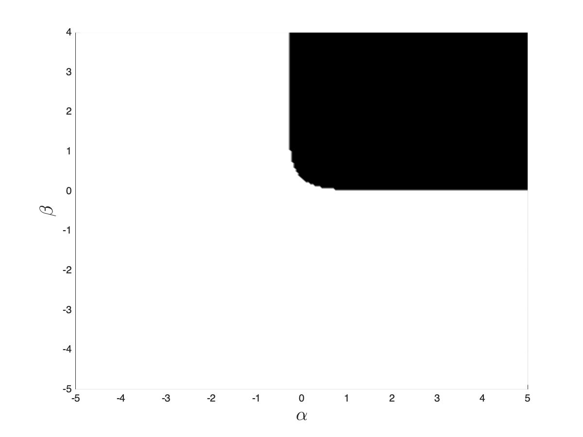
(a) IMEX$1$-DG$1$-S

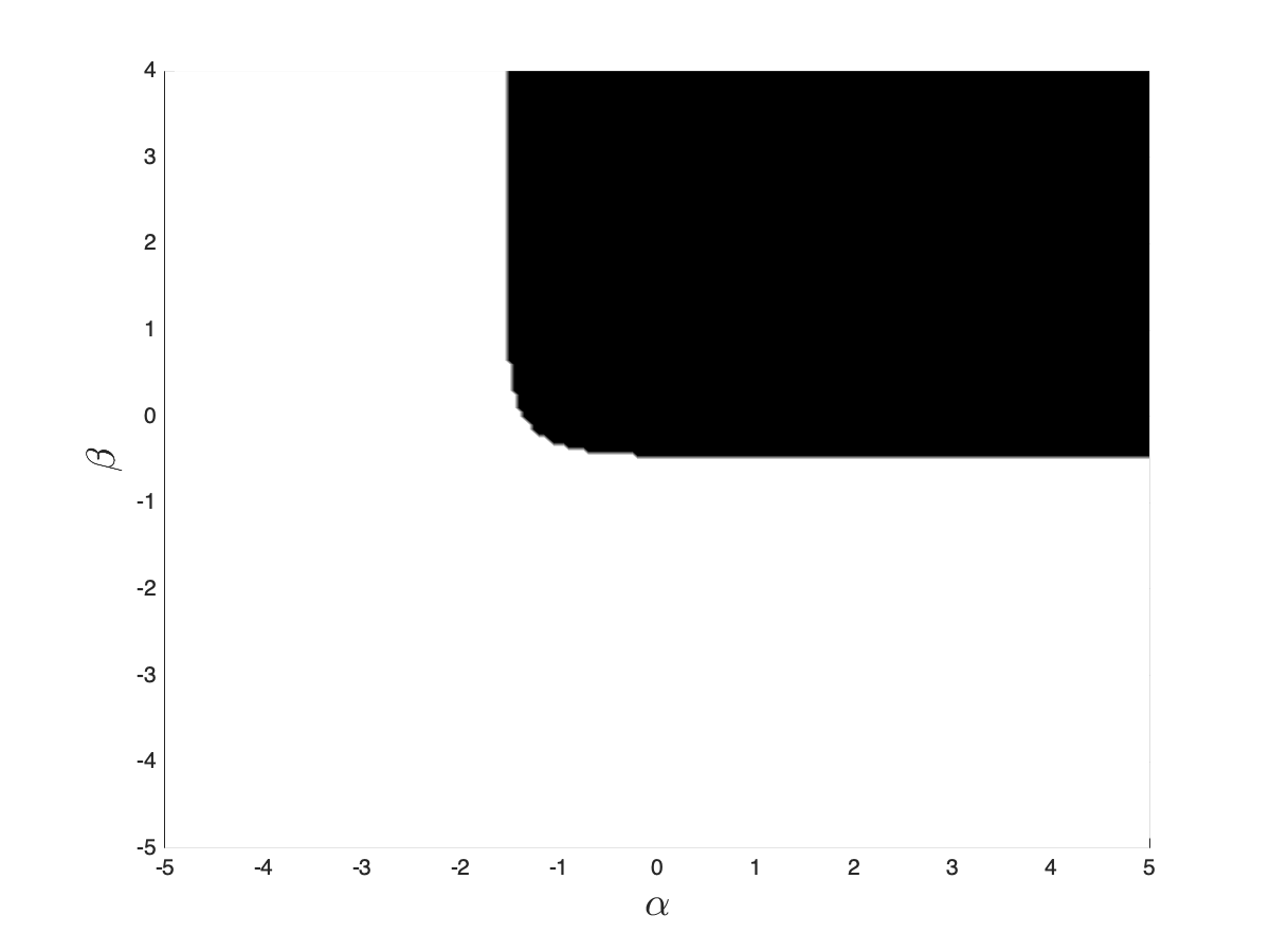
(b) IMEX$2$-DG$2$-S

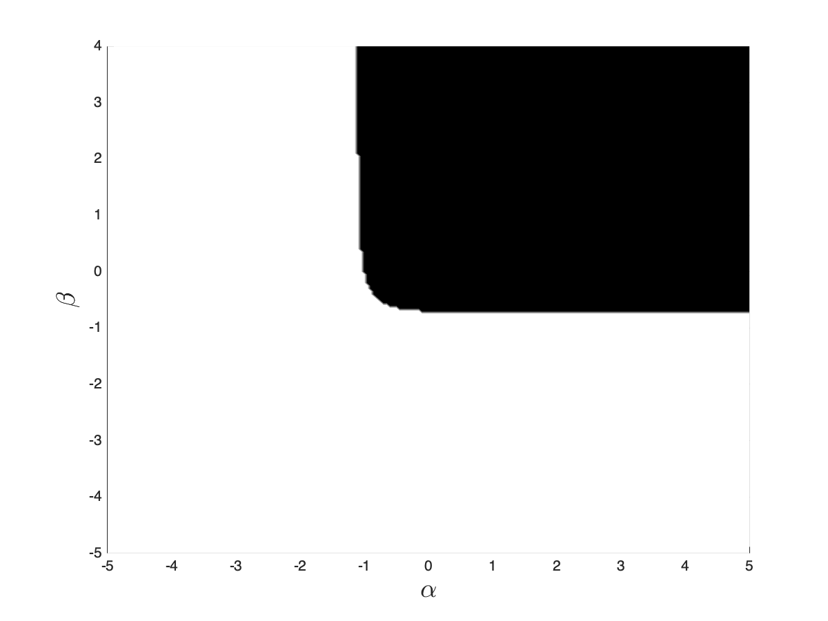
(c) IMEX$3$-DG$3$-S

Figure 5.1: Stability regions of the IMEX$k$-DG$k$-S methods, $k=1,2,3$. White: stable; black: unstable. $\alpha=\log_{10}(\frac{\varepsilon}{\sigma_{m}h})$ and $\beta=\log_{10}(\frac{\Delta t}{\varepsilon h}).$

6 Numerical tests

In this section, we will demonstrate the performance of the IMEX$k$-DG$k$-S scheme, $k=1,2,3$. Two models will be considered. One is the telegraph equation with $\Omega_{v}=\{-1,1\}$ and $\langle f\rangle=\frac{1}{2}(f|_{v=1}+f|_{v=-1})$, the other is the one-group transport equation in slab geometry with $\Omega_{v}=[-1,1]$ and $\langle f\rangle=\frac{1}{2}\int_{-1}^{1}fdv$. For the latter, we discretize the velocity space with $16$ Gaussian quadrature points. The meshes in space are uniform unless otherwise specified.

Based on the energy and Fourier analysis in Section 5, for the one-group transport equation in slab geometry, the time step size $\Delta t$ for the IMEX$k$-DG$k$-S scheme is chosen as $\Delta t_{CFLk}$,

$$\mbox{IMEX1-DG1-S}:\hskip 14.45377pt \Delta t_{CFL1}=\left\{\begin{array}[]{ll}0.75h,&\varepsilon\leq 0.5h,\\ \min(0.75h,\frac{\varepsilon^{2}h}{\varepsilon-0.5h}),&\varepsilon>0.5h,\end{array}\right.$$ (6.1c)

$$\mbox{IMEX2-DG2-S}:\hskip 14.45377pt \Delta t_{CFL2}=\left\{\begin{array}[]{ll}0.75h,&\varepsilon\leq 0.025h,\\ \min(0.75h,\frac{\varepsilon^{2}h/\sqrt{10}}{\varepsilon-0.025h}),&\varepsilon\geq 0.025h,\end{array}\right.$$ (6.1f)

$$\mbox{IMEX3-DG3-S}:\hskip 14.45377pt \Delta t_{CFL3}=\left\{\begin{array}[]{ll}0.75h,&\varepsilon\leq 0.05h,\\ \min(0.75h,\frac{0.1\varepsilon^{2}h}{\varepsilon-0.05h}),&\varepsilon>0.05h.\end{array}\right.$$ (6.1i)

When the schemes are unconditionally stable, $\Delta t=0.75h$ is used to ensure good resolution. The time step conditions in (6.1) also work well for the telegraph equation. We want to mention that, when boundary conditions are Dirichlet (see next subsection), due to the numerical boundary treatment, a smaller time step size is taken for the second order IMEX2-DG2-S scheme in the diffusive regime. For the linear solver, we apply the Schur complement discussed in Section 3.5 and GMRES [24] solver, which is implemented under the framework of C++ library PETSC [2].

6.1 Numerical boundary condition

For some numerical tests, the following inflow (also Dirichlet) boundary conditions are given:

$$f(x_{L},v,t)=f_{L}(v,t),\;\;v\geq 0\quad\text{and}\quad f(x_{R},v,t)=f_{R}(v,t),\;\;v\leq 0.$$

These conditions are insufficient to define the boundary conditions for $\rho=\langle f\rangle$ and $g$, hence numerical treatments are needed. We here adopt a close-loop strategy similar to [10, 21]. For simplicity, we present the strategy using the one-group transport equation in slab geometry with the velocity space being continuous. In implementation, we substitute integrals in $\Omega_{v}$ with their discrete counterparts.

Main idea: Our numerical boundary treatment is based on the following idea. At the left boundary, we set

$$\rho_{L}(t)+\varepsilon g_{L}(v,t)=f_{L}(v,t),\quad v\geq 0\quad\text{(inflow)},$$ (6.2a)

$$\rho_{L}(t)+\varepsilon g_{L}(v,t)=\rho_{h}(x_{\frac{1}{2}}^{+},t)+\varepsilon g_{h}(x_{\frac{1}{2}}^{+},v,t),\quad v<0\quad\text{(outflow)},$$ (6.2b)

$$\langle g_{L}(v,t)\rangle=0.$$ (6.2c)

Integrate (6.2a) in $v$ from $0$ to $1$ and (6.2b) from $-1$ to $0$, and sum them up, we get

$$\rho_{L}=\rho_{L}(t)=\frac{1}{2}\Big{(}\rho_{h}(x_{\frac{1}{2}}^{+},t)+\int_{0}^{1}f_{L}(v,t)dv+\varepsilon\int_{-1}^{0}g_{h}(x_{\frac{1}{2}}^{+},v,t)dv\Big{)},$$ (6.3a)

$$g_{L}=g_{L}(v,t)=\begin{cases}\frac{1}{\varepsilon}(f_{L}(v,t)-\rho_{L}(t)),\;\;v\geq 0,\\ \frac{1}{\varepsilon}(\rho_{h}(x_{\frac{1}{2}}^{+},t)+\varepsilon g_{h}(x_{\frac{1}{2}}^{+},v,t)-\rho_{L}(v,t)),\;\;v<0.\end{cases}$$ (6.3b)

With a similar idea, we obtain at the right boundary

$$\rho_{R}=\rho_{R}(t)=\frac{1}{2}\Big{(}\rho_{h}(x_{N+\frac{1}{2}}^{-},t)+\int_{-1}^{0}f_{R}(v,t)dv+\varepsilon\int_{0}^{1}g_{h}(x_{N+\frac{1}{2}}^{-},v,t)dv\Big{)},$$ (6.4a)

$$g_{R}=g_{R}(v,t)=\begin{cases}\frac{1}{\varepsilon}(\rho_{h}(x_{N+\frac{1}{2}}^{-},t)+\varepsilon g_{h}(x_{N+\frac{1}{2}}^{-},v,t)-\rho_{R}(v,t)),\;\;v\geq 0,\\ \frac{1}{\varepsilon}(f_{R}(v,t)-\rho_{R}(t)),\;\;v<0.\end{cases}$$ (6.4b)

Numerical flux: The boundary strategies are imposed through numerical fluxes. On boundaries, we modify numerical fluxes in (3.7) to be

$$(\breve{\rho_{h}})_{\frac{1}{2}}:=\rho_{L},\;\;\widehat{\langle vg_{h}\rangle}_{\frac{1}{2}}:={\langle vg_{h}\rangle}_{\frac{1}{2}}^{+},\;\;$$ (6.5a)

$$(\breve{\rho_{h}})_{N+\frac{1}{2}}:=\rho_{R},\;\;\widehat{\langle vg_{h}\rangle}_{N+\frac{1}{2}}:={\langle vg_{h}\rangle}_{N+\frac{1}{2}}^{-}+c_{R}(\rho_{R}-\rho_{N+\frac{1}{2}}^{-}),$$ (6.5b)

$$(\widetilde{vg_{h}})_{\frac{1}{2}}:=\left\{\begin{array}[]{ll}{vg_{L}},&\mbox{if}\;v\geq 0\\ ({vg_{h}})_{\frac{1}{2}}^{+},&\mbox{if}\;v<0\end{array}\right.,\quad(\widetilde{vg_{h}})_{N+\frac{1}{2}}:=\left\{\begin{array}[]{ll}({vg_{h}})_{N+\frac{1}{2}}^{-},&\mbox{if}\;v\geq 0\\ vg_{R},&\mbox{if}\;v<0\end{array}\right..$$ (6.5g)

The penalty term $c_{R}(\rho_{R}-\rho_{N+\frac{1}{2}}^{-})$ is added to maintain the accuracy of the schemes, and one can refer to [5, 18] for details on the role of this penalty term. In our simulation, we take $c_{R}=1$.

We want to mention that, due to this numerical boundary treatment, the IMEX$2$-DG$2$-S scheme is no longer unconditionally stable in the diffusive regime. We modify the time step condition in (6.1) with $\Delta t_{CFL2}=0.1h$ when $\varepsilon\leq 0.025h$. Note that this time step condition can still be larger than a parabolic time step condition $\Delta t=O(h^{2})$.

6.2 Numerical examples

Example 1: smooth example [21]. We consider the one-group transport equation in slab geometry with a smooth example on $\Omega_{x}=[0,2\pi]$. The initial conditions are

$$\rho(x,0)=\sin(x),\qquad g(x,v,0)=-v\cos(x),$$

with periodic boundary conditions, and $\sigma_{s}=1$, $\sigma_{a}=0$. $\Omega_{x}$ is partitioned with a uniform mesh and we define $N=\frac{(x_{R}-x_{L})}{h}$. Numerical errors in $L_{\infty}$-norm and convergence orders are obtained by Richardson extrapolation:

$$E^{\rho}_{N}=||\rho_{h}(x,T)-\rho_{\frac{h}{2}}(x,T)||_{L_{\infty}(\Omega_{x})},\quad\text{and},\quad O^{\rho}_{N}=log_{2}(E^{\rho}_{N}/E^{\rho}_{2N}),$$ (6.6a)

$$E^{g}_{N}=\max_{j=1,\dots N_{v}}||g_{h}(x,v_{j},T)-g_{\frac{h}{2}}(x,v_{j},T)||_{L_{\infty}(\Omega_{x})},\quad\text{and},\quad O^{g}_{N}=log_{2}(E^{g}_{N}/E^{g}_{2N}).$$ (6.6b)

Numerical results at $T=1$ with $\varepsilon=0.5$, $\varepsilon=10^{-2}$ and $\varepsilon=10^{-6}$ are shown in Tables 6.1-6.3. We observe that the IMEX$k$-DG$k$-S scheme, $k=1,2,3$, has the optimal $k$-th order accuracy that seems to be uniform in $\varepsilon$.

Table 6.1: Errors and convergence orders for the example 1, IMEX1-DG1-S

$\varepsilon$	$N$	$E^{\rho}_{N}$	order	$E_{N}^{g}$	order
0.5	10	1.921E-02	-	1.909E-02	-
	20	8.709E-02	1.14	8.390E-03	1.19
	40	3.540E-02	1.30	3.699E-03	1.18
	80	1.619E-03	1.13	1.744E-03	1.08
	160	7.737E-04	1.07	8.469E-04	1.04
$10^{-2}$	10	1.029E-02	-	1.467E-02	-
	20	4.371E-03	1.23	6.742E-03	1.12
	40	2.014E-03	1.12	3.204E-03	1.07
	80	9.648E-04	1.06	1.553E-03	1.04
	160	5.265E-04	0.87	7.986E-04	0.96
$10^{-6}$	10	1.011E-02	-	1.459E-02	-
	20	4.306E-03	1.23	6.709E-03	1.12
	40	1.988E-03	1.12	3.189E-03	1.07
	80	9.520E-04	1.06	1.546E-03	1.04
	160	4.657E-04	1.03	7.618E-04	1.02

Table 6.2: Errors and convergence orders for the example 1, IMEX2-DG2-S

$\varepsilon$	$N$	$E^{\rho}_{N}$	order	$E_{N}^{g}$	order
0.5	10	3.505E-02	-	3.911E-02	-
	20	8.916E-03	1.97	9.991E-03	1.97
	40	2.205E-03	2.02	2.590E-03	1.95
	80	5.479E-04	2.01	6.563E-04	1.98
	160	1.365E-04	2.01	1.650E-04	1.99
$10^{-2}$	10	3.519E-02	-	4.215E-02	-
	20	8.763E-03	2.01	8.869E-03	2.25
	40	2.206E-03	2.00	2.283E-03	1.96
	80	5.523E-04	2.00	5.906E-04	1.95
	160	1.381E-04	2.00	1.536E-04	1.94
$10^{-6}$	10	3.518E-02	-	3.482E-02	- -
	20	8.726E-03	2.01	8.629E-03	2.01
	40	2.195E-03	1.99	2.172E-03	1.99
	80	5.494E-04	2.00	5.435E-04	2.00
	160	1.374E-04	2.00	1.360E-04	2.00

Table 6.3: Errors and convergence orders for the example 1, IMEX3-DG3-S

$\varepsilon$	$N$	$E^{\rho}_{N}$	order	$E_{N}^{g}$	order
0.5	10	2.588E-03	-	2.676E-03	-
	20	3.215E-04	3.01	4.103E-04	2.71
	40	4.028E-05	3.00	6.495E-05	2.66
	80	5.036E-06	3.00	9.198E-06	2.82
	160	6.303E-07	3.00	1.22E-06	2.91
$10^{-2}$	10	2.510E-03	-	2.543E-03	-
	20	3.214E-04	2.97	3.724E-04	2.77
	40	4.039E-05	2.99	1.109E-04	1.75
	80	5.061E-06	3.00	5.292E-06	4.39
	160	6.328E-07	3.00	6.659E-07	2.99
	320	7.910E-08	3.00	8.355E-08	2.99
$10^{-6}$	10	2.505E-03	-	2.554E-03	-
	20	3.211E-04	2.96	3.174E-04	3.01
	40	4.041E-05	2.99	3.998E-05	3.00
	80	5.060E-06	3.00	5.007E-06	3.00
	160	6.327E-07	3.00	6.269E-07	3.00

Example 2: two-material problem [15, 16]. We consider a two-material problem on $\Omega_{x}=[0,11]$ and $\Omega_{v}=[-1,1]$ with isotropic inflow boundary conditions. The setup is as follows.

$$\sigma_{s}=0,\;\;\sigma_{a}=1,\;\;\text{if}\;x\in[0,1],$$

$$\sigma_{s}=100,\;\;\sigma_{a}=0,\;\;\text{if}\;x\in[1,11],$$

$$f_{L}(v,t)=5,\;\;f_{R}(v,t)=0,\;\;f(x,v,0)=0,\;\;$$ (6.7)

and $\varepsilon=1$. We examine the numerical solutions at a shorter time $T=1.5$ and also the steady state solution obtained at $T=20000$. This problem has a pure absorbing region with the length of one mean-free path on the left and a pure scattering region with the length of $1000$ mean-free path on the right. Subregiones with different scales coexist. From the left boundary, an isotropic inflow enters the computational region, and it instantly becomes anisotropic. An interior layer is formed near the interface between the absorbing region and the scattering region.

We use a non-uniform mesh with $h=h^{(1)}=\frac{1}{20}$ on $[0,1]$ and $h=h^{(2)}=\frac{1}{2}$ on $[1,11]$, and the time step $\Delta t$ is determined by (6.1) using $h=h^{(1)}$. With this example, we also want to compare the performance of the IMEX$k$-DG$k$-S schemes proposed here and the IMEX$k$-LDG$k$ schemes in [21] with the weight function $\omega=\exp(-\frac{\varepsilon}{100h})|_{h=h^{(1)}}$. Numerical results are shown in Figure 6.2 and Figure 6.3. The reference solution is obtained by the first order forward Euler upwind finite difference scheme applied to the original kinetic equation (1.1) with $h=\frac{11}{20000}$ and $\Delta t=10^{-5}$ for $T=1.5$, and with $h=\frac{11}{2000}$ and $\Delta t=10^{-4}$ for $T=20000$.

At $T=1.5$, our proposed schemes capture the solutions very well. The third order IMEX3-LDG3-S scheme has the best result. We observe that the IMEX$k$-DG$k$-S schemes outperform the IMEX$k$-LDG$k$ schemes with the chosen weight. Unlike for IMEX$k$-LDG$k$ schemes, one does not need to choose a weight function for our proposed methods for this example when both transport dominant and diffusion dominant regions coexist.

At $T=20000$ when the solution reaches its steady state, the numerical solutions by the IMEX$k$-DG$k$-S scheme, $k=1,2,3$ match the reference solutions well, and they are comparable with those in [21] by IMEX$k$-LDG$k$ scheme. Higher order schemes lead to better resolution as expected.

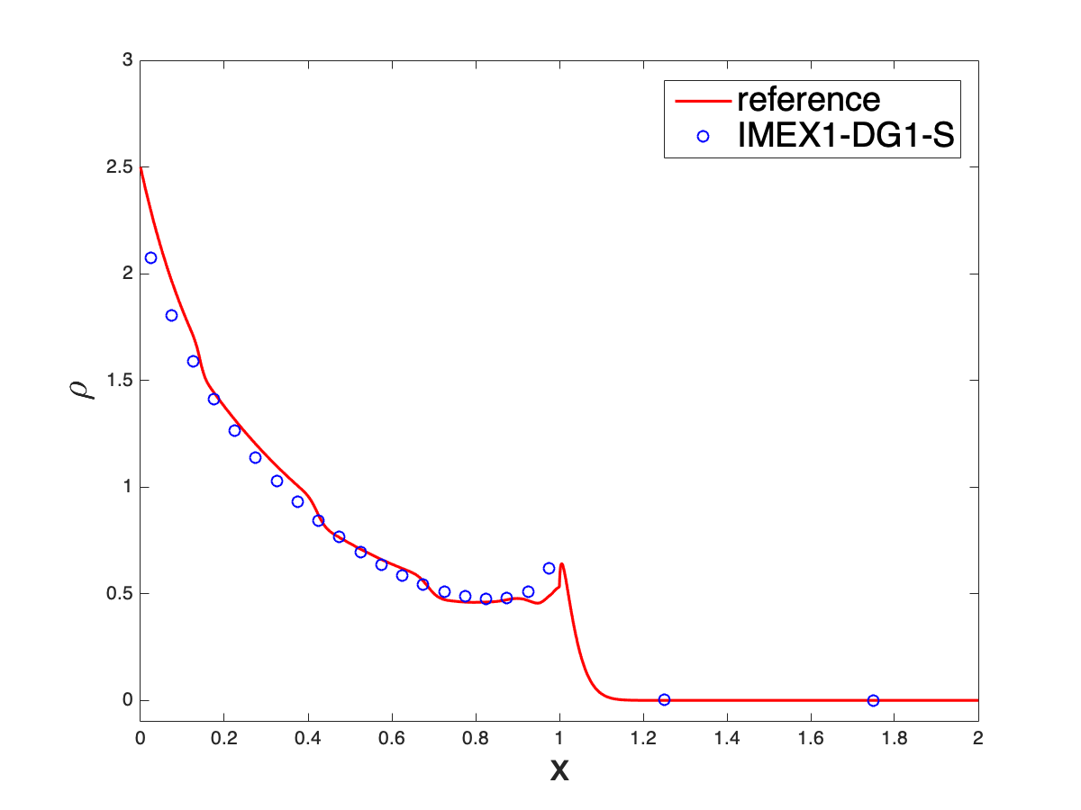
(a) $\rho$, IMEX$1$-DG$1$-S

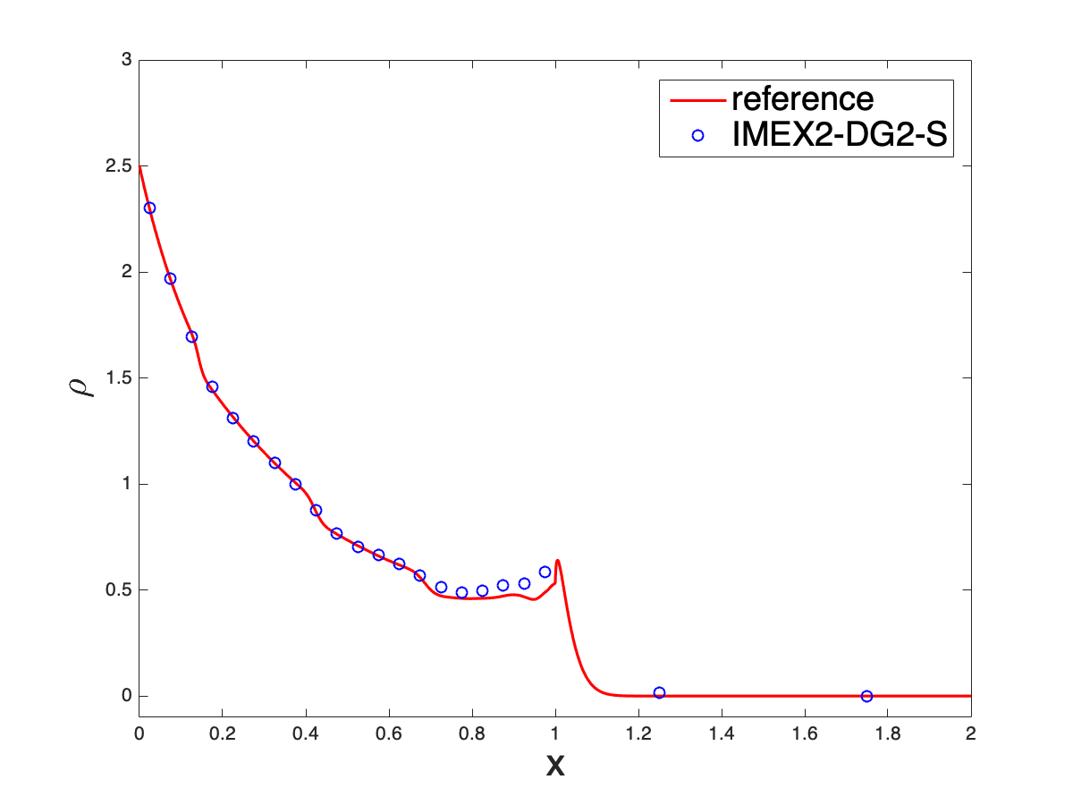
(b) $\rho$, IMEX$2$-DG$2$-S

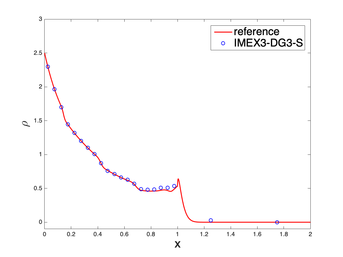
(c) $\rho$, IMEX$3$-DG$3$-S

(d) $\rho$, IMEX$1$-LDG$1$

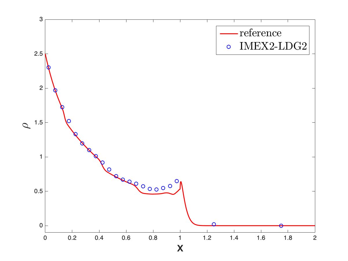
(e) $\rho$, IMEX$2$-LDG$2$

(f) $\rho$, IMEX$3$-LDG$3$

Figure 6.2: Example 2: two-material problem $T=1.5$, zoomed in with $x\in[0,2]$.

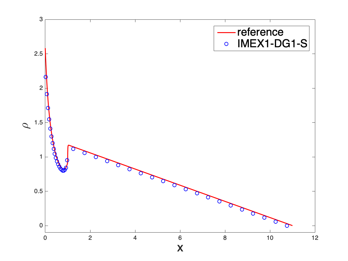
(a) $\rho$, IMEX$1$-DG$1$-S

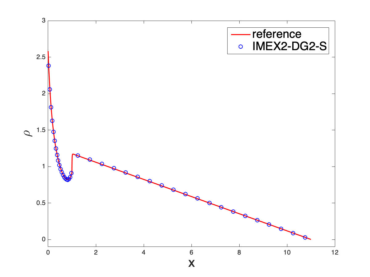
(b) $\rho$, IMEX$2$-DG$2$-S

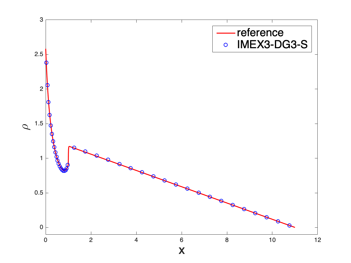
(c) $\rho$, IMEX$3$-DG$3$-S

Figure 6.3: Example 2: two-material problem, $T=20000$, $x\in[0,11]$.

Example 3: problem with varying scattering frequency and constant source term [16]. We consider the one-group transport equation in slab geometry with a source term $G$:

$$\varepsilon\partial_{t}f+v\partial_{x}f=-\frac{\sigma_{s}}{\varepsilon}(\langle f\rangle-f)+\varepsilon\sigma_{a}f+\varepsilon G.$$ (6.8)

The computational domain is $\Omega_{x}=[0,1]$, and

$$\sigma_{s}(x)=1+100x^{2},\;\;\sigma_{a}=0,\;\;G=1,\;\;$$

$$f_{L}(v,t)=0,\;\;f_{R}(v,t)=0,\;\;f(x,v,0)=0,\;\;\varepsilon=10^{-2}.$$ (6.9)

The effective scaling is determined by $\frac{\varepsilon}{\sigma_{s}(x)}$, hence, it is varying in the computational domain.

We use a uniform mesh with $h=\frac{1}{40}$ and the source term $G$ is treated explicitly. Numerical results for $T=0.4$ are presented in Figure 6.4. The reference solution is obtained by the first order forward Euler upwind finite difference scheme applied to (1.1) with $h=\frac{1}{20000}$ and $\Delta t=0.1\varepsilon h$. As the value of $\sigma_{s}(x)$ is larger on the right, the scattering effect is stronger on that side. As a result, sharp feature exists near the right boundary. All schemes match the reference solution well on this relatively coarse mesh, and high order schemes perform better, especially near the right boundary.

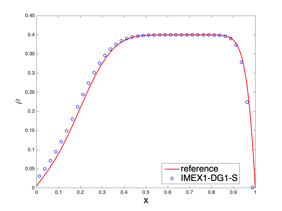
(a) $\rho$, IMEX$1$-DG$1$-S

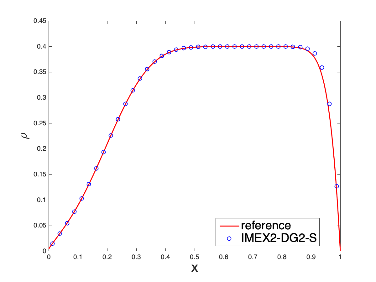
(b) $\rho$, IMEX$2$-DG$2$-S

(c) $\rho$, IMEX$3$-DG$3$-S

Figure 6.4: Example 3: changing scattering problem for one-group transport equation, $T=0.4$.

Example 4: diffusive and kinetic regime with isotropic inflow Dirichlet boundary conditions [3, 16]. In this example, we consider the one-group transport equation in slab geometry on $\Omega_{x}=[0,1]$, and

$$\sigma_{s}=1,\;\;\sigma_{a}=0,\;\;f_{L}(v,t)=1,\;\;f_{R}(v,t)=0,\;\;f(x,v,0)=0,$$ (6.10)

with $\varepsilon=1,10^{-8}$.

In Figure 6.5, we report numerical results on a uniform mesh with $h=\frac{1}{40}$. The reference solution for $\varepsilon=1$ is obtained by the first order forward Euler upwind finite difference scheme applied to (1.1) with $h=\frac{1}{2000}$ and $\Delta t=0.5\varepsilon h$, while the reference solution for $\varepsilon=10^{-8}$ is obtained by a central difference scheme solving the diffusion limit (2.2) with $h=\frac{1}{2000}$ and $\Delta t=0.25h^{2}$. For comparison, we also include in Figure 6.5 the numerical results by the IMEX$k$-LDG$k$ schemes in [21] with the weight function $\omega=\exp(-\frac{\varepsilon}{h})$ and $\omega=1$, and when $\varepsilon=1$ .

When the problem is relatively kinetic with $\varepsilon=1$, it is observed that the numerical solutions by the proposed methods match the reference solutions well. The results are comparable with that by the IMEX$k$-LDG$k$ methods with the weight function $\omega=\exp({-\frac{\varepsilon}{h}})$, and both are better than that by the IMEX$k$-LDG$k$ methods with the constant weight function $\omega=1$. Note that in this example, the initial and boundary conditions at $x=0$ are not compatible, and this introduces a Dirac delta structure in $\partial_{x}\rho$ at $t=0$ and subsequently sharper features in the solution form near the left boundary. All these pose challenge to approximate the weighted diffusion term $\omega\partial_{xx}\rho$, unless $\omega$ is chosen to be small to balance the term $\partial_{xx}\rho$. This explains the IMEX$k$-LDG$k$ schemes with the weight function $\omega=\exp(-\frac{\varepsilon}{h})$ outperform that with $\omega=1$. Our IMEX-DG-S schemes on the other hand do not have a weight function to tune for this example.

When the problem is relatively diffusive with $\varepsilon=10^{-8}$, we take $\Delta t=0.25h$ in the diffusive regime, instead of the original $\Delta t=0.75h$ in (6.1) (still stable), for both the IMEX1-DG1-S and IMEX3-DG3-S schemes. The numerical solutions by the IMEX$k$-DG$k$-S scheme, $k=1,2,3$, match the reference solutions well. The higher order schemes lead to better resolution.

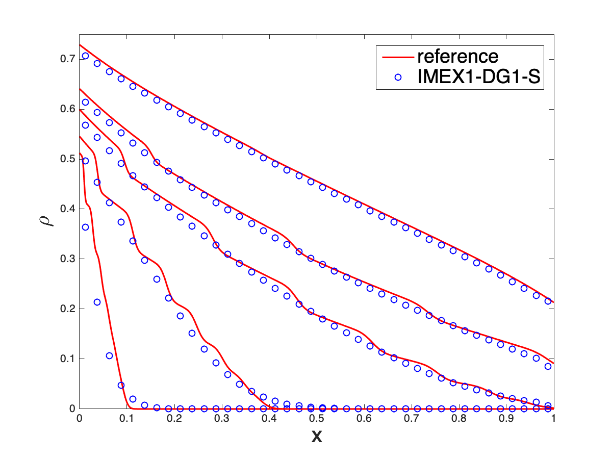
(a) $\rho$ for $\varepsilon=1$, IMEX$1$-DG$1$-S

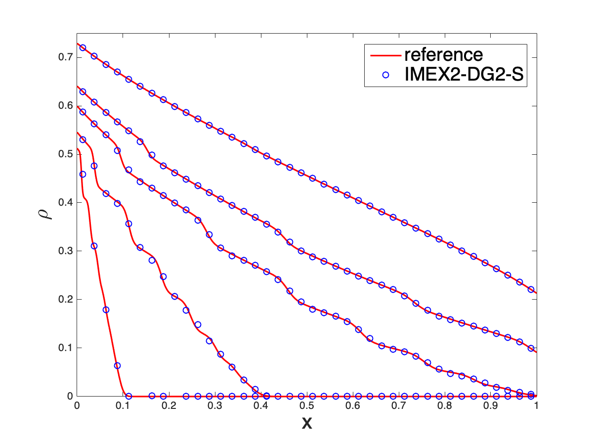
(b) $\rho$ for $\varepsilon=1$, IMEX$2$-DG$2$-S

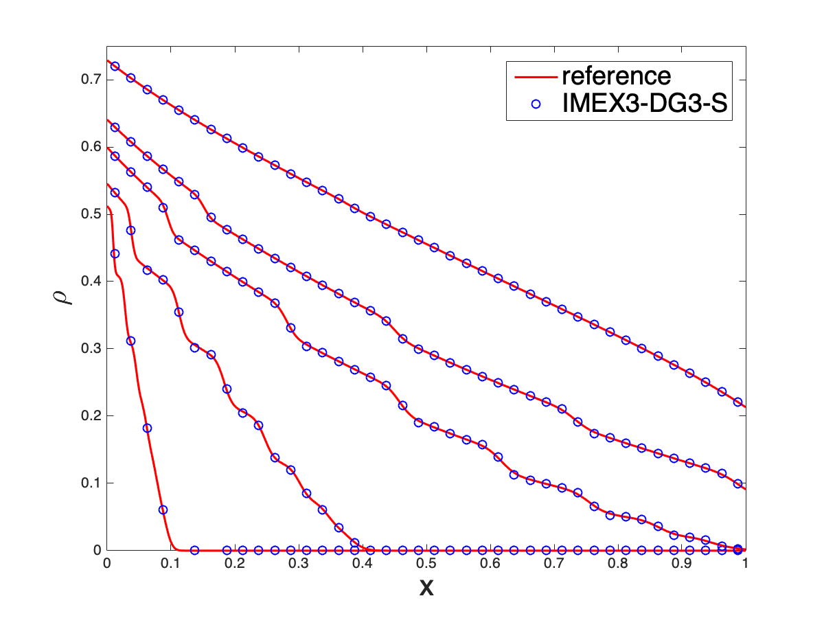
(c) $\rho$ for $\varepsilon=1$, IMEX$3$-DG$3$-S

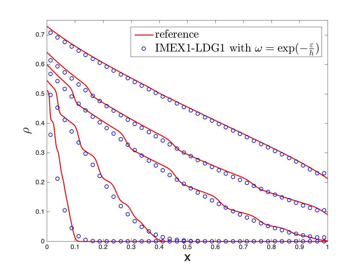
(d) $\rho$ for $\varepsilon=1$, IMEX$1$-LDG$1$ with $\omega=\exp(-\frac{\varepsilon}{h})$

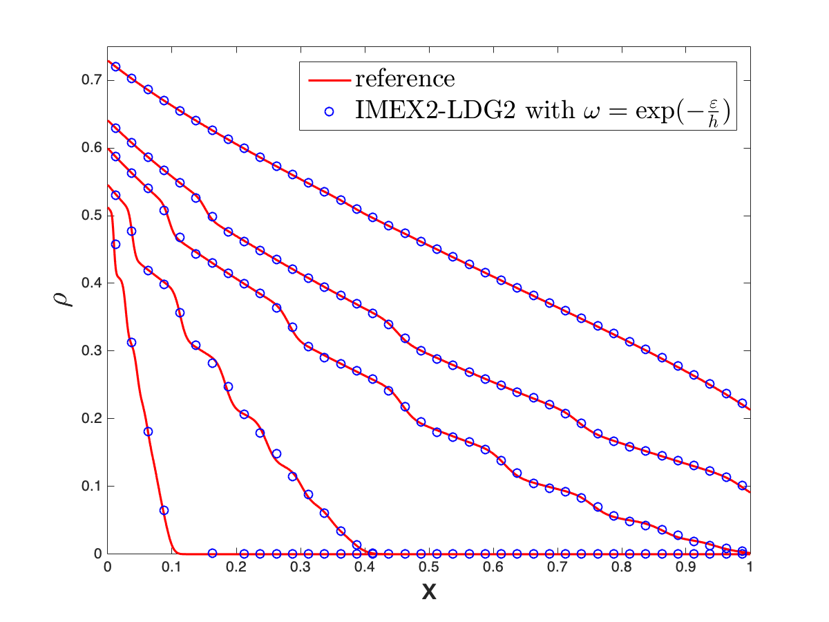
(e) $\rho$ for $\varepsilon=1$, IMEX$2$-LDG$2$ with $\omega=\exp(-\frac{\varepsilon}{h})$

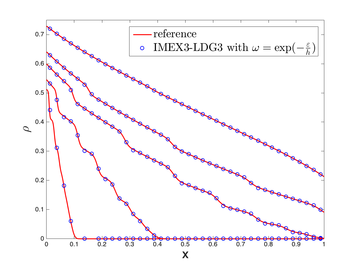
(f) $\rho$ for $\varepsilon=1$, IMEX$3$-LDG$3$ with $\omega=\exp(-\frac{\varepsilon}{h})$

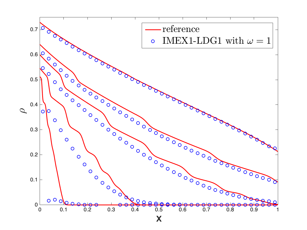
(g) $\rho$ for $\varepsilon=1$, IMEX$1$-LDG$1$ with $\omega=1$

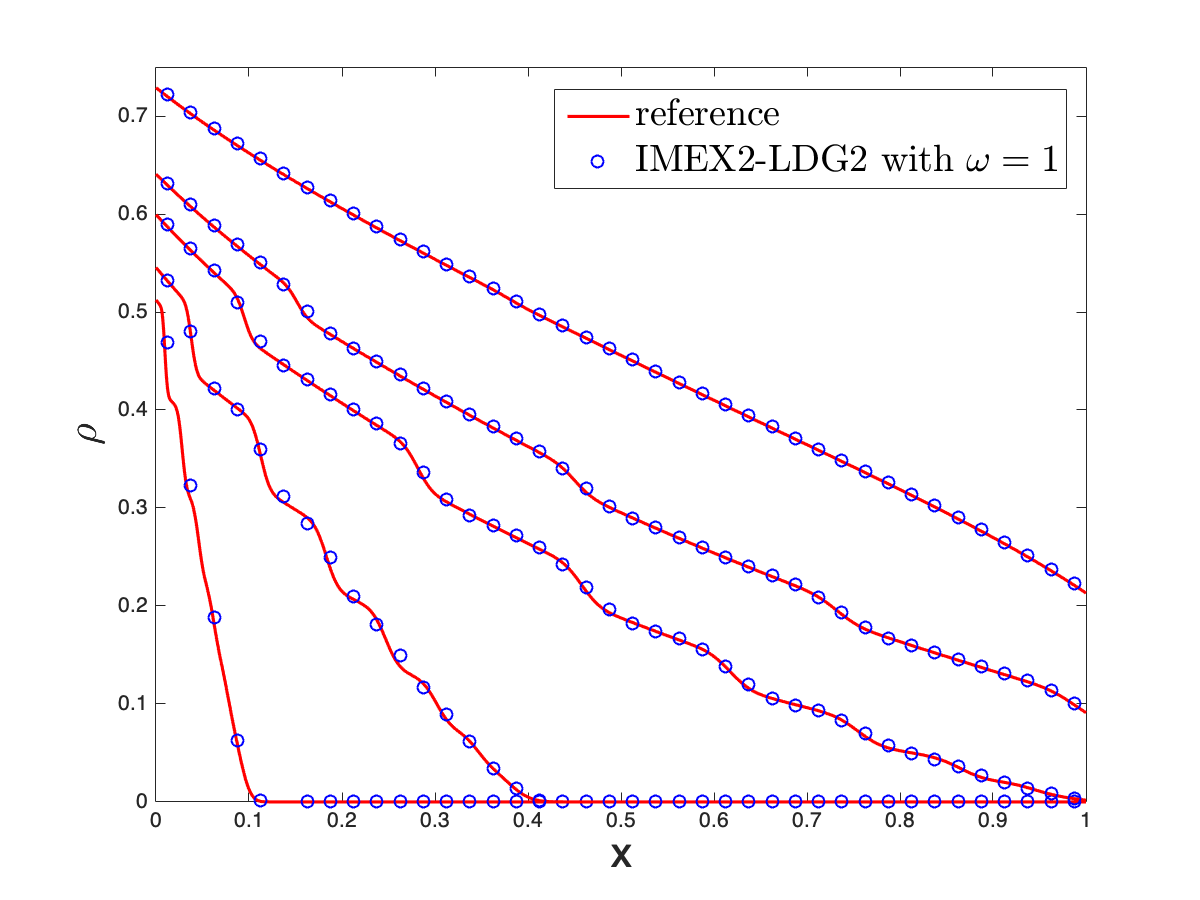
(h) $\rho$ for $\varepsilon=1$, IMEX$2$-LDG$2$ with $\omega=1$

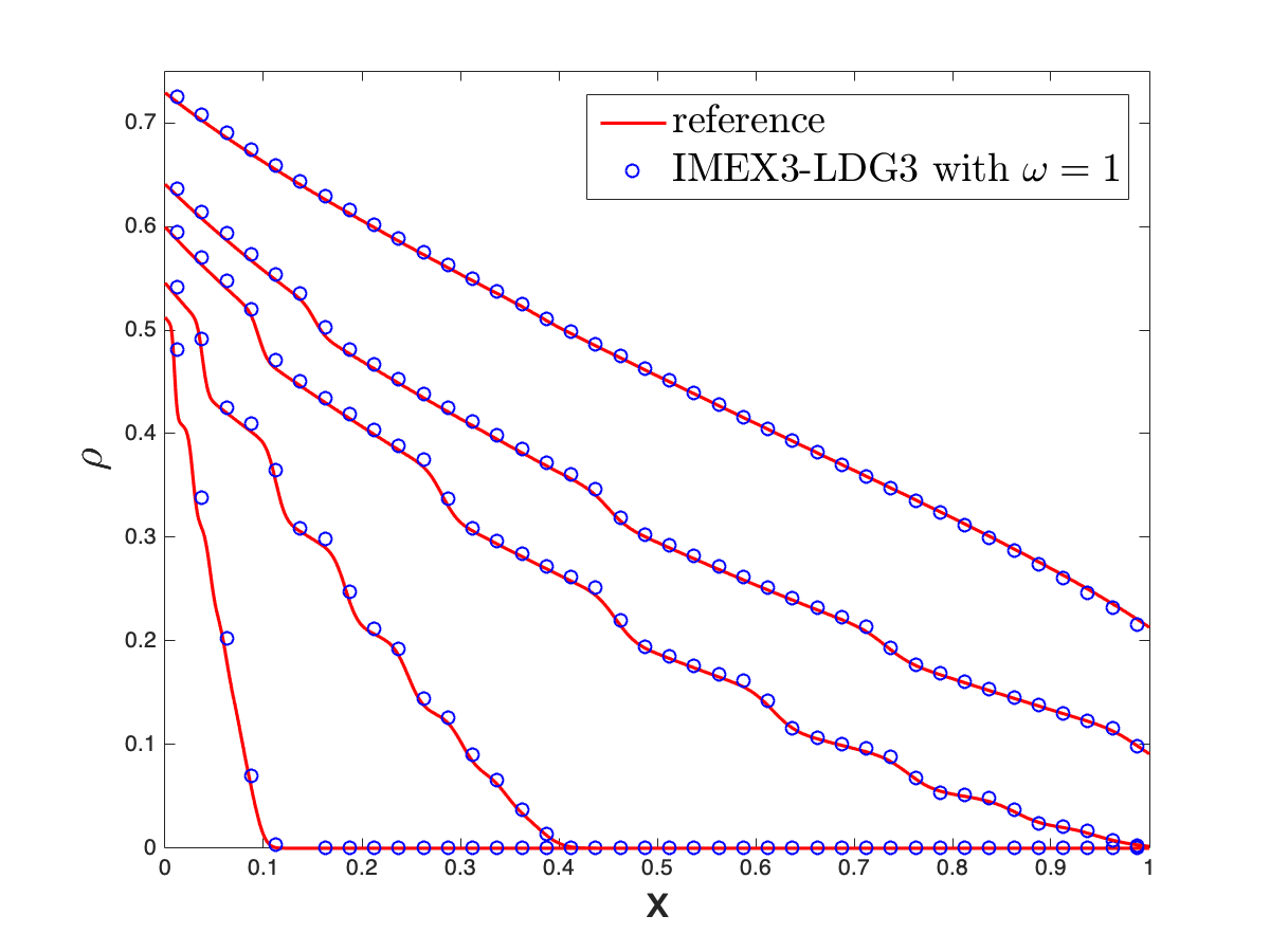
(i) $\rho$ for $\varepsilon=1$, IMEX$3$-LDG$3$ with $\omega=1$

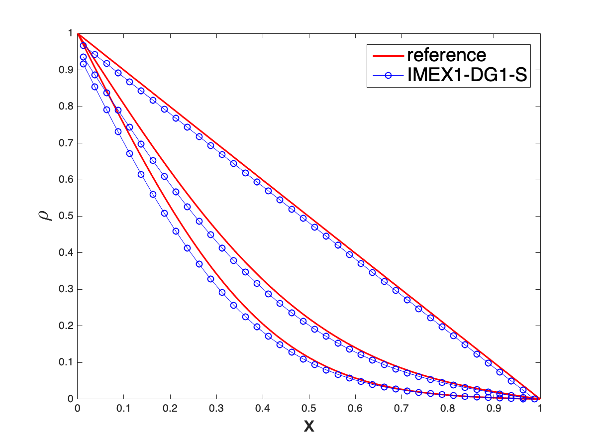
(j) $\rho$ for $\varepsilon=10^{-8}$, IMEX$1$-DG$1$-S

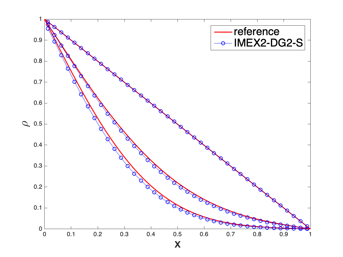
(k) $\rho$ for $\varepsilon=10^{-8}$, IMEX$2$-DG$2$-S

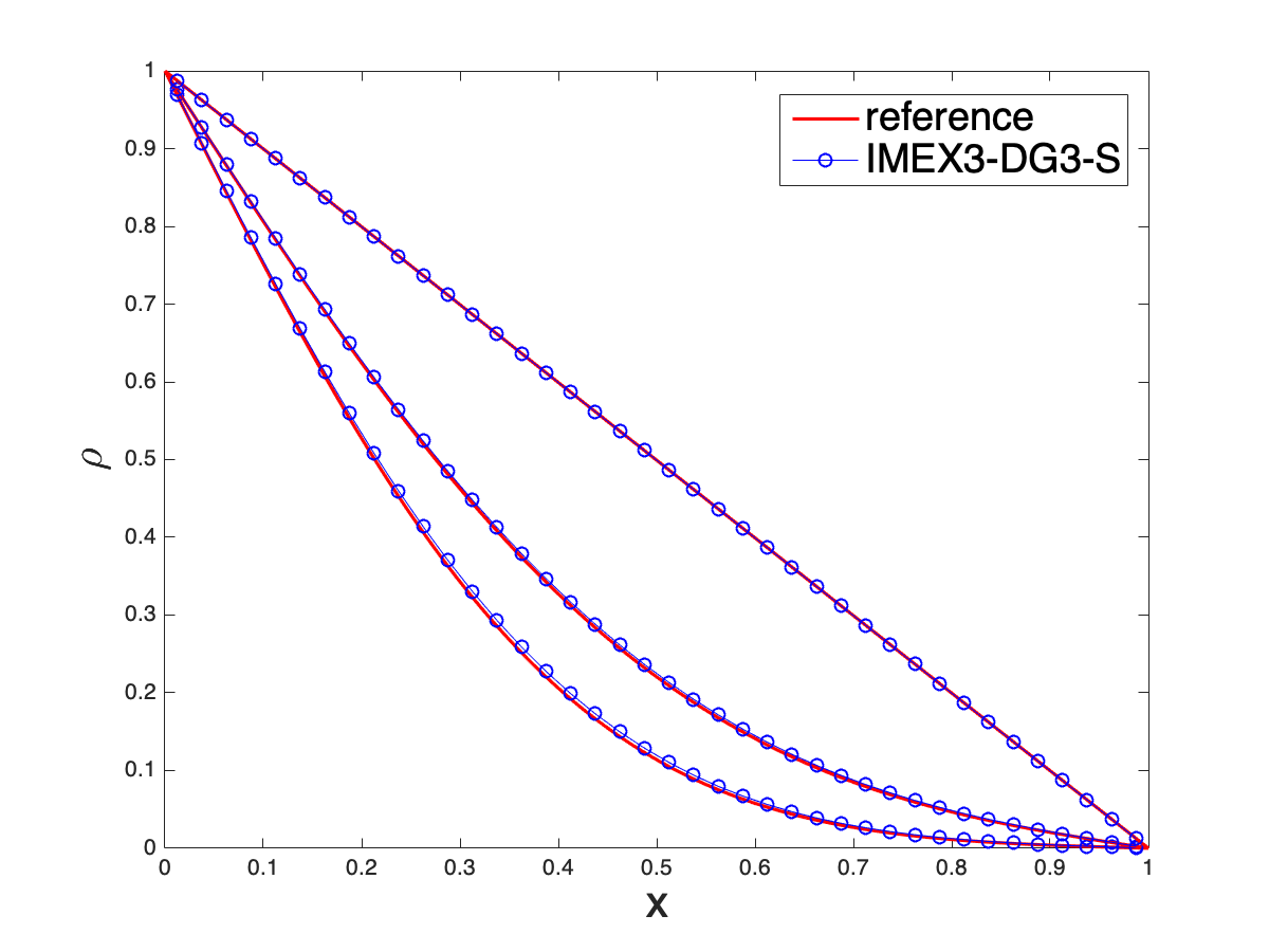
(l) $\rho$ for $\varepsilon=10^{-8}$, IMEX$3$-DG$3$-S

Figure 6.5: Example 4: diffusive and kinetic regime with isotropic inflow Dirichlet boundary conditions for one-group transport equation. Top three rows: $\rho$ for $\varepsilon=1$ and $T=0.1,\;0.4,\;1.0,\;1.6,\;4.0$; Bottom row: $\rho$ for $\varepsilon=10^{-8}$ and $T=0.15,\;0.25,\;2.0$.

Example 5: Riemann problem for telegraph equation [3, 10]. We consider a Riemann problem with $\Omega_{v}=\{-1,1\}$, $\sigma_{s}=1$, $\sigma_{a}=0$ and the initial data

$$\begin{cases}\rho(x,0)=2,\;g(x,v,0)=0,\;x\leq 0,\\ \rho(x,0)=1,\;g(x,v,0)=0,\;x>0.\end{cases}$$ (6.11)

Two different cases are considered: the more kinetic case with $\varepsilon=0.7$ and $\Omega_{x}=[-1,1]$, and the more diffusive case with $\varepsilon=10^{-6}$ and $\Omega_{x}=[-2,2]$. For both, a uniform partition of $\Omega_{x}$ with $h=\frac{1}{40}$ is used, and the final time is set as $T=0.15$. Numerical results for $\rho$ and $j(x,t)=\langle vg\rangle$ are presented in Figure 6.6 and Figure 6.7. The reference solution for $\varepsilon=0.7$ is obtained by the first order forward Euler upwind finite difference scheme solving (1.1) with a uniform mesh $h=\frac{1}{1000}$ and $\Delta t=0.05\varepsilon h$. The reference solution for $\varepsilon=10^{-6}$ is calculated by a central difference scheme solving the diffusion limit (2.2) with $h=\frac{1}{1000}$ and $\Delta t=0.25h^{2}$.

For the kinetic case with $\varepsilon=0.7$, results from all schemes match the reference solution well. Compared with the first order scheme, the second and the third order schemes give less dissipative results and capture the sharp features better. Small oscillation near discontinuity can be further reduced by applying nonlinear limiters. With the discontinuity present in the solution, when IMEX-LDG schemes are applied to this example (see Section 6.1.2 in [21]), the quality of the computed solutions really depends on the choice of the weight function. For the diffusive case with $\varepsilon=10^{-6}$, all schemes capture the solution well, and high order schemes show better resolutions.

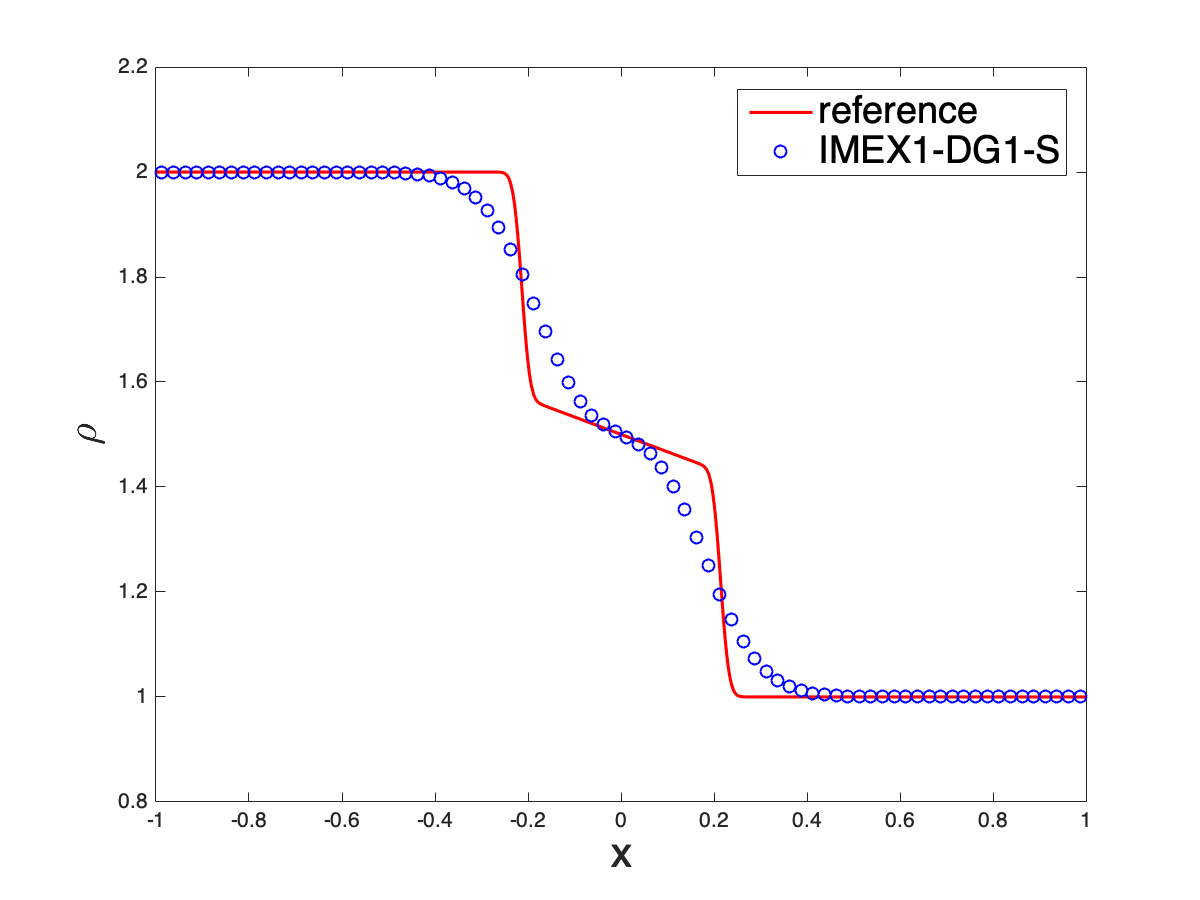
(a) $\rho$, IMEX$1$-DG$1$-S

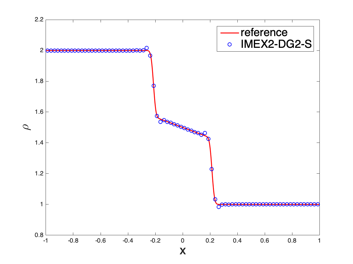
(b) $\rho$, IMEX$2$-DG$2$-S

(c) $\rho$, IMEX$3$-DG$3$-S

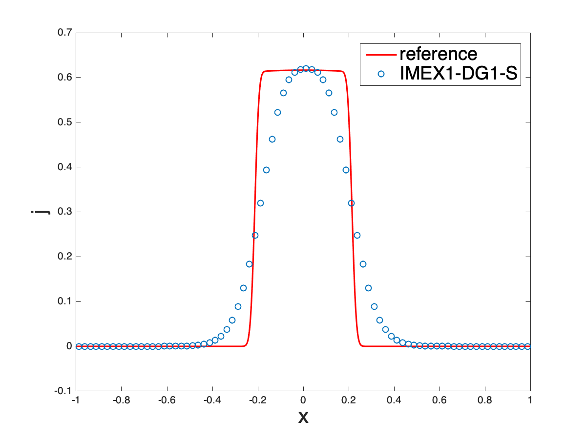
(d) $j$, IMEX$1$-DG$1$-S

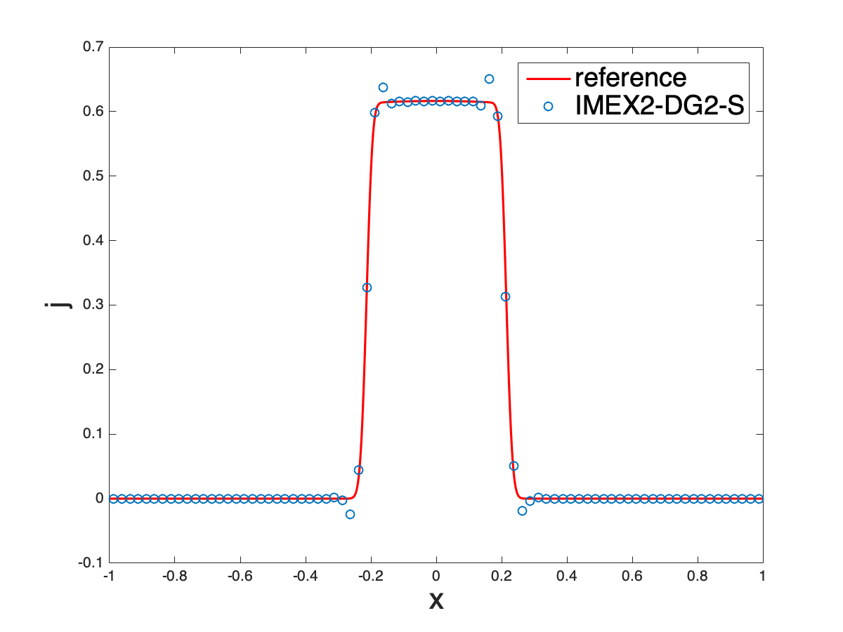
(e) $j$, IMEX$2$-DG$2$-S

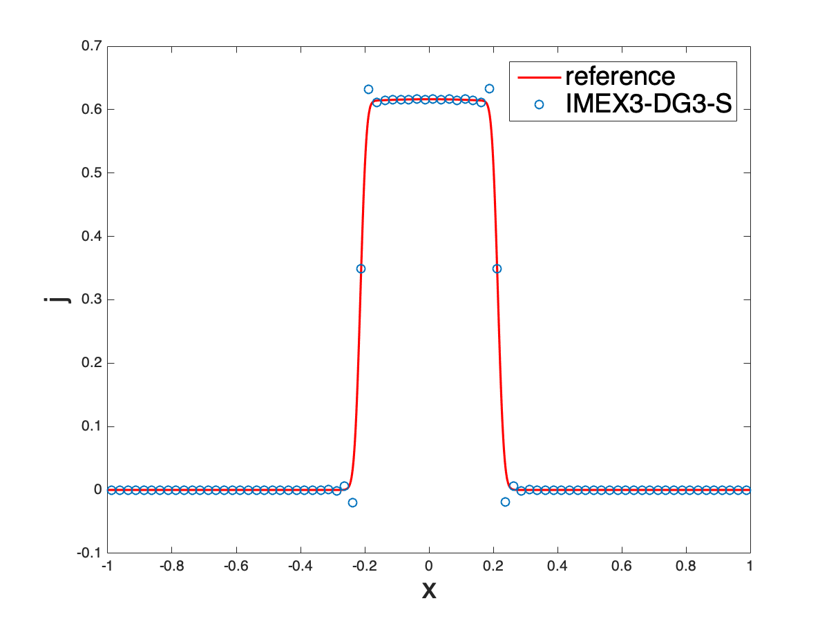
(f) $j$, IMEX$3$-DG$3$-S

Figure 6.6: Example 5: Riemann problem for the telegraph equation. $\varepsilon=0.7$ and $T=0.15$.

(a) $\rho$, IMEX$1$-DG$1$-S

(b) $\rho$, IMEX$2$-DG$2$-S

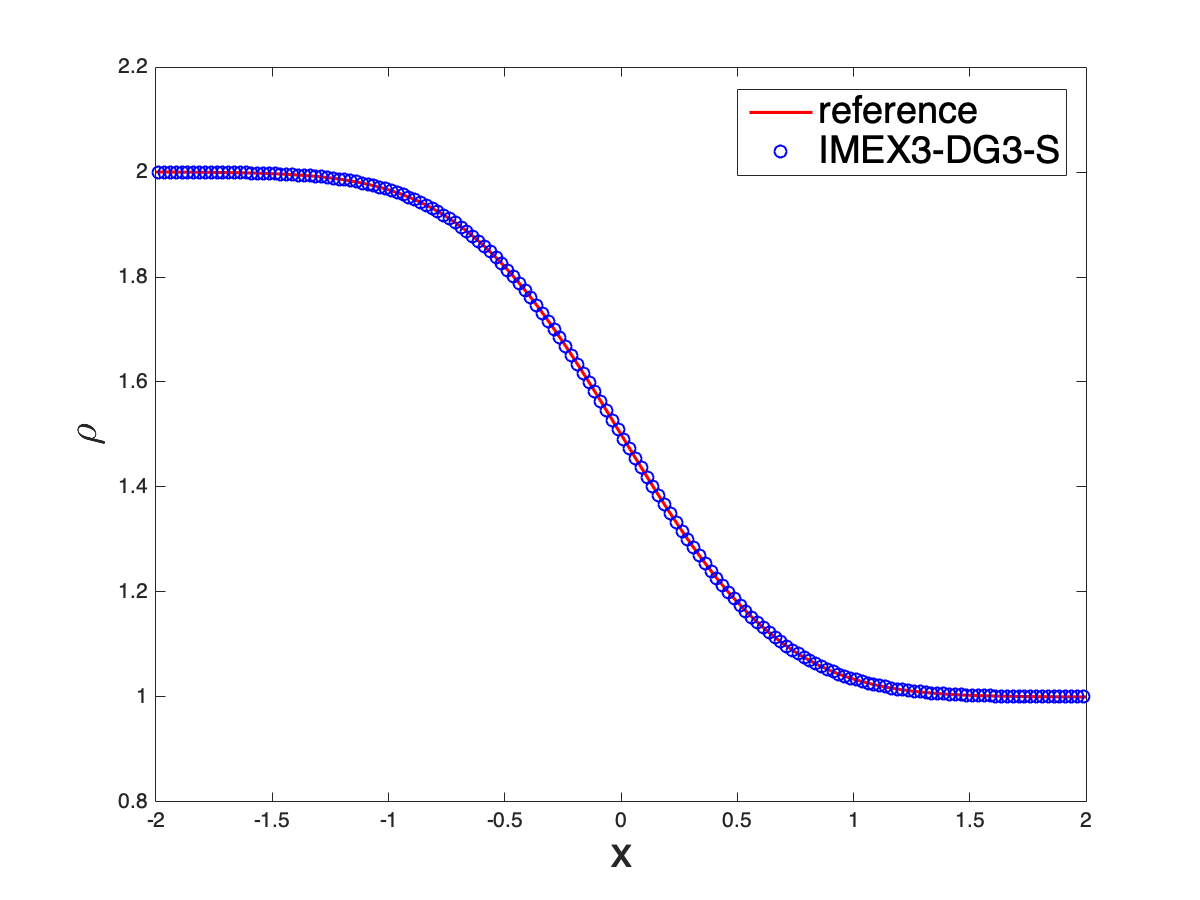
(c) $\rho$, IMEX$3$-DG$3$-S

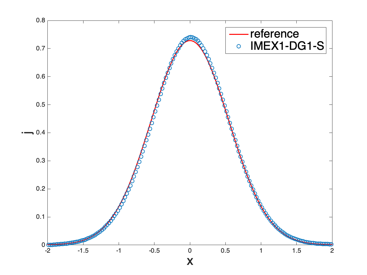
(d) $j$, IMEX$1$-DG$1$-S

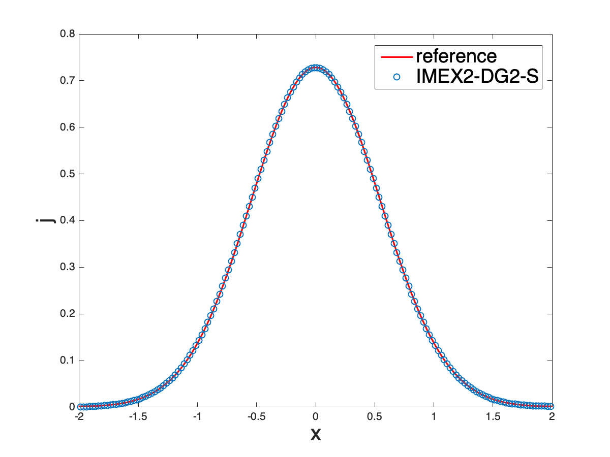
(e) $j$, IMEX$2$-DG$2$-S

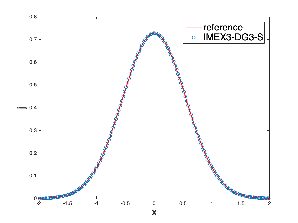
(f) $j$, IMEX$3$-DG$3$-S

Figure 6.7: Example 5: Riemann problem for telegraph equation. $\varepsilon=10^{-6}$ and $T=0.15$.

7 Conclusions

To design AP schemes with unconditional stability in the diffusive regime, numerical schemes are developed in [3, 21] based on an additional reformulation to the decomposed system. The key of the additional reformulation is to introduce a weighted diffusive term. In this paper, to avoid issues related to the ad-hoc choice of the weight function, we design IMEX-DG-S schemes by applying a new implicit-explicit temporal strategy. Asymptotic analysis confirms the AP property of the proposed schemes. Energy type stability analysis for the IMEX1-DG1-S scheme and Fourier type stability analysis for the IMEX$k$-DG$k$-S scheme, $k=1,2,3$, are presented. These analyses verify uniform stability of the schemes with respect to $\varepsilon$ and unconditional stability in the diffusive regime. To achieve these AP and stability properties with computational cost similar to the IMEX-LDG schemes in [21], the Schur complement is applied on the linear solver level. Numerical examples are presented to demonstrate the performance of the IMEX-DG-S schemes and their advantages over the weight-dependent IMEX-LDG schemes in [21].

References

- [1] U.M. Ascher, S.J. Ruuth, and R.J. Spiteri. Implicit-explicit Runge-Kutta methods for time-dependent partial differential equations. Applied Numerical Mathematics, 25(2):151–167, 1997.
- [2] Satish Balay, Shrirang Abhyankar, Mark Adams, Jed Brown, Peter Brune, Kris Buschelman, Lisandro Dalcin, Alp Dener, Victor Eijkhout, W Gropp, et al. PETSc users manual. 2019.
- [3] Sebastiano Boscarino, Lorenzo Pareschi, and Giovanni Russo. Implicit-explicit Runge–Kutta schemes for hyperbolic systems and kinetic equations in the diffusion limit. SIAM Journal on Scientific Computing, 35(1):A22–A51, 2013.
- [4] Russel E Caflisch, Shi Jin, and Giovanni Russo. Uniformly accurate schemes for hyperbolic systems with relaxation. SIAM Journal on Numerical Analysis, 34(1):246–281, 1997.
- [5] Paul Castillo, Bernardo Cockburn, Dominik Schötzau, and Christoph Schwab. Optimal a priori error estimates for the -version of the local discontinuous galerkin method for convection–diffusion problems. Mathematics of Computation, 71(238):455–478, 2002.
- [6] Bernardo Cockburn, George E Karniadakis, and Chi-Wang Shu. Discontinuous Galerkin methods: theory, computation and applications, volume 11. Springer Science & Business Media, 2012.
- [7] Bernardo Cockburn and Chi-Wang Shu. The local discontinuous Galerkin method for time-dependent convection-diffusion systems. SIAM Journal on Numerical Analysis, 35(6):2440–2463, 1998.
- [8] Pierre Degond. Asymptotic-preserving schemes for fluid models of plasmas. arXiv preprint arXiv:1104.1869, 2011.
- [9] Juhi Jang, Fengyan Li, Jing-Mei Qiu, and Tao Xiong. Analysis of asymptotic preserving DG-IMEX schemes for linear kinetic transport equations in a diffusive scaling. SIAM Journal on Numerical Analysis, 52(4):2048–2072, 2014.
- [10] Juhi Jang, Fengyan Li, Jing-Mei Qiu, and Tao Xiong. High order asymptotic preserving DG-IMEX schemes for discrete-velocity kinetic equations in a diffusive scaling. Journal of Computational Physics, 281:199–224, 2015.
- [11] Shi Jin. Asymptotic preserving (AP) schemes for multiscale kinetic and hyperbolic equations: a review. Lecture Notes for Summer School on “Methods and Models of Kinetic Theory (M&MKT), Porto Ercole (Grosseto, Italy), pages 177–216, 2010.
- [12] Shi Jin, Lorenzo Pareschi, and Giuseppe Toscani. Diffusive relaxation schemes for multiscale discrete-velocity kinetic equations. SIAM Journal on Numerical Analysis, 35(6):2405–2439, 1998.
- [13] Shi Jin, Lorenzo Pareschi, and Giuseppe Toscani. Uniformly accurate diffusive relaxation schemes for multiscale transport equations. SIAM Journal on Numerical Analysis, 38(3):913–936, 2000.
- [14] Axel Klar. An asymptotic-induced scheme for nonstationary transport equations in the diffusive limit. SIAM journal on numerical analysis, 35(3):1073–1094, 1998.
- [15] Edward W. Larsen and Jim E. Morel. Asymptotic solutions of numerical transport problems in optically thick, diffusive regimes II. Journal of Computational Physics;(USA), 83(1), 1989.
- [16] Mohammed Lemou and Luc Mieussens. A new asymptotic preserving scheme based on micro-macro formulation for linear kinetic equations in the diffusion limit. SIAM Journal on Scientific Computing, 31(1):334–368, 2008.
- [17] Elmer Eugene Lewis and Warren F Miller. Computational methods of neutron transport. John Wiley & Sons, New York, 1984.
- [18] Jichun Li, Cengke Shi, and Chi-Wang Shu. Optimal non-dissipative discontinuous Galerkin methods for Maxwell’s equations in Drude metamaterials. Computers & Mathematics with Applications, 73(8):1760–1780, 2017.
- [19] Tai-Ping Liu and Shih-Hsien Yu. Boltzmann equation: micro-macro decompositions and positivity of shock profiles. Communications in Mathematical Physics, 246(1):133–179, 2004.
- [20] Giovanni Naldi and Lorenzo Pareschi. Numerical schemes for kinetic equations in diffusive regimes. Applied mathematics letters, 11(2):29–35, 1998.
- [21] Zhichao Peng, Yingda Cheng, Jing-Mei Qiu, and Fengyan Li. Stability-enhanced AP IMEX-LDG schemes for linear kinetic transport equations under a diffusive scaling. Journal of Computational Physics, page 109485, 2020.
- [22] Zhichao Peng, Yingda Cheng, Jing-Mei Qiu, and Fengyan Li. Stability-enhanced AP IMEX1-LDG method: energy-based stability and rigorous AP property. arxiv:2005.05454, 2020.
- [23] Gerald C. Pomraning. The equations of radiation hydrodynamics. International Series of Monographs in Natural Philosophy, Oxford: Pergamon Press, 1973.
- [24] Youcef Saad and Martin H Schultz. GMRES: A generalized minimal residual algorithm for solving nonsymmetric linear systems. SIAM Journal on scientific and statistical computing, 7(3):856–869, 1986.
- [25] Fuzhen Zhang. The Schur complement and its applications, volume 4. Springer Science & Business Media, 2006.