Can $\overline{\rm{MS}}$ parton distributions be negative?

It is common lore that Parton Distribution Functions (PDFs) in the $\overline{\rm{MS}}$ factorization scheme can become negative beyond leading order due to the collinear subtraction which is needed in order to define partonic cross sections. We show that this is in fact not the case and next-to-leading order (NLO) $\overline{\rm{MS}}$ PDFs are actually positive in the perturbative regime. In order to prove this, we modify the subtraction prescription, and perform the collinear subtraction in such a way that partonic cross sections remain positive. This defines a factorization scheme in which PDFs are positive. We then show that positivity of the PDFs is preserved when transforming from this scheme to $\overline{\rm{MS}}$, provided only the strong coupling is in the perturbative regime, such that the NLO scheme change is smaller than the LO term.

1 Parton distributions from the parton model to QCD

In the naive parton model parton distribution functions (PDFs) are probability densities for a parton to carry a given fraction of their parent hadron’s momentum. This simple picture remains true at leading order (LO) in QCD where each PDF is proportional to a physically measurable (in principle) cross section: it can consequently still be viewed as a probability and it is non-negative. We will henceforth refer to the property of being non-negative as “positivity” (while really meaning “positive-semidefiniteness”).

As is well known [1], positivity of the PDFs is in general violated at higher perturbative orders, where physical cross sections are the convolution of the PDFs with a partonic cross section. Partonic cross sections are beset by collinear singularities, whose subtraction and factorization into the PDF spoils in general the separate positivity of the subtracted partonic cross sections and of the PDFs. Therefore, the positivity condition on PDFs beyond LO becomes a positivity constraint of physical observables [1, 2]. When determining PDFs from data, this constraint must be imposed on physical observables, rather than PDFs themselves: for instance by using Lagrange multipliers, or pseudodata for suitable positivity observables, such as for example hypothetical deep-inelastic structure functions corresponding to gauge bosons that couple to only one quark flavor [3].

These positivity constraint may have a significant impact on PDF determination, especially in regions where there are little or no direct constraints coming from experimental data. For example, in a recent study of the strange PDF [4] it was found that adding to the dataset a positivity constraint for the charm structure function $F_{2}^{c}$ significantly impacts the flavor decomposition of the quark sea in the large $x$ region. However, adding positivity constraints in this way, as constraints on pseudo-observables, is cumbersome from a methodological point of view, and theoretically not satisfactory. Indeed, as the target accuracy of the PDFs increases, and PDFs are used more and more for new physics studies and searches in regions in which the PDFs are experimentally unconstrained, it becomes necessary to enforce an increasingly elaborate set of positivity constraints [5, 6] for a set of suitably chosen and tuned pseudo-observables. This poses obvious problems of fine-tuning. In fact, universality of PDFs suggests that positivity constraints should be imposed in a process-independent way, without having to rely on a specific choice of processes, and therefore, that it ought to be possible to impose the constraint at the level of PDFs.

Here, we address this issue head-on by constructing a subtraction scheme in which PDFs are positive, and which we refer to as a “positive” factorization scheme. We do this by studying the way collinear subtraction is performed in the $\overline{\rm{MS}}$ scheme, and showing that negative partonic cross sections arise as a consequence of over-subtraction of a positive contribution. This is chiefly due to the fact that the subtraction is performed at a scale which, as the kinematic threshold for production of the final state is approached, is higher than the actual physical scale; and also, in gluonic channels, due to the way the $d$-dimensional averaging over gluon polarizations is treated in dimensional regularization.

Once these effects are taken into account it is possible to formulate a subtraction prescription such that partonic cross sections remain positive. Effectively, this choice of subtraction corresponds to a “physical” scheme, in which the scale choice is directly related to the scale of parton radiation. Of course, the positive factorization scheme is not unique, since any further scheme change through a matrix with positive entries (“positive matrix”, henceforth) would leave the partonic cross sections positive. It is then possible to show that there exist schemes in which PDFs also remain positive, so that the positive hadronic cross section is obtained by convoluting positive partonic cross sections with positive PDFs.

The availability of positive schemes can be advantageous in the context of PDF determination. Indeed, if PDFs are parametrized in the positive scheme, positivity can be enforced by choice of parametrization. Results in the commonly used $\overline{\rm{MS}}$ scheme can then be obtained by scheme transformation.

However, perhaps surprisingly, this turns out not to be necessary: indeed, using the explicit form of the scheme change matrix from the positive scheme to $\overline{\rm{MS}}$ it is easy to prove that in the perturbative region PDFs remain positive in $\overline{\rm{MS}}$. Hence, the common lore that $\overline{\rm{MS}}$ PDFs might be negative beyond LO turns out to be incorrect. Positivity of the fitted PDFs can then be imposed using the standard methodology in the $\overline{\rm{MS}}$ scheme.

The paper is organized as follows. In Section 2 we show how negative partonic cross sections arise due to over-subtraction. We start with the prototypical case of deep-inelastic scattering (DIS): we review the computation of coefficient functions at next-to-leading order (NLO); we show how over-subtraction arises in the $\overline{\rm{MS}}$ scheme and how it can be fixed by choosing a suitable subtraction prescription; we then discuss how this works in the general case of hadronic processes, where we can define a “positive” subtraction prescription which preserves positivity of all partonic cross sections. In Sect. 3 we then turn to positivity of PDFs: first, we use our positive subtraction prescription to define a positive factorization scheme; then we show how positivity of PDFs is preserved in this factorization scheme; and finally by studying the transformation from the positive scheme to $\overline{\rm{MS}}$ we prove that positivity is preserved in $\overline{\rm{MS}}$ in the perturbative regime. The bulk of our discussion will be at NLO, and its validity beyond NLO will be addressed in the end of Sect. 3.

2 Positivity of partonic cross sections

QCD factorization allows expressing physical cross sections $\sigma$ as convolutions of partonic cross sections with parton distributions $f_{i}$. In the prototypical case of DIS the cross section is expressed in terms of hadronic structure functions $F(x,Q^{2})$, which are then factorized in terms of parton-level structure functions, called coefficient functions $C_{i}$:

$$\frac{1}{x}F(x,Q^{2})=\sum_{i}e^{2}_{i}C_{i}\otimes f_{i},$$ (1)

where the sum runs over all parton species, $e_{i}$ are quark electric charges, or the sum over all electric charges for the gluon, (for photon-induced DIS, and more in general electroweak charges), $\otimes$ denotes convolution, and we refer to Ref. [7] for notations and conventions. The convolution in Eq. (1) links the three a priori physically distinct scaling variables on which respectively the physical observable $F$, the partonic cross-section $C$ and the PDF $f$ depend. In the sequel, for clarity, we will denote with $x$ the physically observable variable (Bjorken-$x$ for DIS, or the scaling variable in hadronic collisions), with $z$ the variable on which the coefficient function depends, and with $\xi$ the PDF momentum fraction. Of course, Mellin transformation turns the convolution into an ordinary product and upon transformation all these variables are mapped onto the same $N$ variable.

At LO all factors on the right-hand side of Eq. (1) are manifestly positive. Indeed, the partonic cross sections (which for DIS at LO are trivial) are defined as the square modulus of amplitudes. The PDFs in turn are defined as operator matrix elements which can be interpreted as probability distributions [8, 9]: for quark PDFs [8]

$$f_{i}(\xi)=\frac{1}{4\pi}\int dy^{-}e^{-i\xi P^{+}y^{-}}\langle P|\bar{\psi}_{i}(0,y^{-},\vec{0}_{T})\gamma^{+}{\cal P}\exp\left[ig_{s}\int_{0}^{y^{-}}d\bar{y}^{-}A_{a}^{+}(0,\bar{y}^{-},\vec{0}_{T})\frac{1}{2}\lambda_{a}\right]\psi_{i}(0)|P\rangle,$$ (2)

where ${\cal P}$ denotes path-ordering; $P$ is the four-momentum of the parent hadron in light-cone components and $g_{s}$ is the strong coupling, with analogous expressions for antiquarks and gluons [8]. It can be shown (see e.g. Sect. 6.7 of Ref. [10]) that the expression Eq. (2) is a number density, and as such before subtraction of divergences it is positive.

Beyond LO, besides ultraviolet renormalization, both the PDFs and the partonic cross section are beset by collinear singularities which can be factored into the PDF. Before factorization the PDF is a “bare” probability density $f_{i}^{(0)}$ [10], while after factorization it is a renormalized PDF $f_{i}$

$$f_{i}=\sum_{j}Z^{S}_{ij}\otimes f_{j}^{(0)}.$$ (3)

In operator language, the factor $Z^{S}_{ij}$ is a multiplicative renormalization of the operator Eq. (2), which admits a perturbative expansion

$$Z^{S}_{ij}(Q^{2})=\delta_{ij}+\frac{\alpha_{s}}{2\pi}\delta^{S}_{ij}(Q^{2})+O(\alpha_{s}^{2}),$$ (4)

where $\delta^{S}_{ij}$ is a counterterm which diverges after regularization is removed, the superscript $S$ denotes the fact that the finite part of the counterterm depends on the choice of a particular subtraction scheme $S$, and regularization induces a dependence of the counterterm and thus of the renormalization constant on scale.

The counterterm can be determined in a standard way by taking the matrix element of the operator in a state in which the right-hand side of Eq. (2) is perturbatively computable, such as a free state of a parton $i$, in which the PDF for finding a parton $j$ is trivially

$$f_{j}^{i\,(0)}(\xi)=\delta_{ij}\delta(1-\xi),$$ (5)

imposing a renormalization condition and finally removing the regulator. In practice, this is most easily done [10, 9] by introducing a probe that couples to the free quark, so for instance computing the structure function Eq. (1) for deep-inelastic scattering off a free quark. This is the strategy that we will follow in this section, where such a computation will be performed explicitly in a way that fully determines the factorization scheme, both in the $\overline{\rm{MS}}$ and in our new positive schemes.

The factorization argument then works as follows. The $d$-dimensional structure function Eq. (1) is written as

$$\frac{1}{x}F_{i}(x,Q^{2},\epsilon) =\sum_{j}e^{2}_{j}C_{j}\otimes f_{j}^{i\,(0)}$$ (6)

$$=\sum_{j}e^{2}_{j}C_{j}^{S}\otimes f_{j}^{i\,S};\qquad\quad d=4-2\epsilon,$$ (7)

and computed by taking in turn the incoming parton to be each of the parton species, i.e. using Eq. (5). Of course, the structure function on the l.h.s. then reduces to the unsubtracted, regularized coefficient function, which is essentially the cross-section for scattering off the given incoming free parton. The counterterm is defined by imposing the cancellation of the singularity. Up to NLO, assuming a free incoming parton according to Eq. (5), substituting in Eqs. (6-7) the perturbative expression Eq. (4) of the renormalization factor Eq. (3), and assuming a perturbative expansion of the coefficient functions of the form

$$C_{i}(z,Q^{2})=C^{(0)}_{i}(z,Q^{2})+\frac{\alpha_{s}}{2\pi}C^{(1)}_{i}(z,Q^{2})+O(\alpha_{s}^{2})$$ (8)

one gets

$$C_{i}^{S}(z,Q^{2},\epsilon)={C^{(1)}_{i}}(z,Q^{2},\epsilon)-\delta_{qi}^{S}(z,Q^{2},\epsilon)\,,$$ (9)

where $q$ denotes a quark parton. Note that, up to NLO, imposing finiteness of the DIS structure functions fixes the renormalization in the quark sector because DIS is a probe that only couples to quarks at leading order.

The advantage of determining the counterterms in this way, as opposed to performing a direct computation of the current matrix element Eq. (2) is that in operator matrix elements all divergences appear as ultraviolet, while, when computing a structure function for an incoming free parton (or, more generally, a generic partonic cross-section), collinear singularities come from the infrared region of integration over transverse momenta. Hence, one may compute the relevant cross-section using renormalized perturbation theory (i.e., with counterterms already included in the Lagrangian). The only divergences are then of collinear and infrared origin. The regularized partonic cross-section is then finite if the computation is performed with $\epsilon<0$, and it enjoys the positivity properties of a standard cross-section. This property will be crucial in the argument presented below.

After the subtraction Eq. (9), the partonic cross-section (coefficient function) is finite in the $\epsilon\to 0$ limit, so one may define the four-dimensional coefficient function as

$${C^{(1)}_{i}}^{S}(z)=\lim_{\epsilon\to 0^{-}}\left({C^{(1)}_{i}}(z,Q^{2},\epsilon)-\delta_{qi}^{S}(z,Q^{2},\epsilon)\right),$$ (10)

where $\epsilon\to 0^{-}$ denotes the fact that the limit is taken from below, as discussed above. Note that the four-dimensional coefficient function function can depend only on $z$ for dimensional reasons, while the $d$ dimensional one also depends on $Q^{2}$ through the combination $\frac{Q^{2}}{\mu^{2}}$, where $\mu^{2}$ is the scale of dimensional regularization. That this subtraction is always possible is the content of factorization theorems [10, 9]. The universal (i.e. process-independent) nature of the collinear singularities ensure that the renormalization conditions on parton distributions, defined as operator matrix elements Eq. (2) without reference to any specific process, may be determined by the computation of a particular process or set of processes as discussed here.

The finite part of the subtraction is arbitrary and it defines the factorization scheme $S$. In $\overline{\rm{MS}}$ it turns out that in some partonic subchannels the subtracted cross section can be negative: effectively, negative finite parts are factored away from the regularized cross sections, and into the PDFs. These can then also become negative, though whether this happens or not depends on the relative weight of the various subchannels. On the other hand, the residue of the collinear pole is universal—it is given by process-independent splitting functions—and this makes it possible to define its subtraction in a way that preserves positivity of the partonic cross section at the regularized level. If all contributions which are factored away from the partonic cross section and into the PDF remain positive, then the latter also stays positive.

Having explained the general strategy, we now implement it explicitly. We first discuss DIS structure functions. We then turn to hadronic processes, both quark-induced and gluon induced.

2.1 Deep-inelastic coefficient functions

At NLO, photon-induced DIS proceeds through the two sub-processes $q+\gamma^{*}\to X$ and $g+\gamma^{*}\to X$, in such a way that the contribution of each quark or antiquark flavor to the structure function $F_{2}$ can be written as:

$$\frac{1}{x}F_{2}(x,Q^{2})=e_{q}^{2}\left[q+\frac{\alpha_{s}}{2\pi}\left(C^{(1)}_{q}\otimes q+C^{(1)}_{g}\otimes g\right)\right](Q^{2})\,,$$ (11)

where $e_{q}$ is the electric charge of the quark, on the right-hand side we have omitted the $x$ dependence which arises from the convolution, and the generalization to $Z$- and $W$-induced DIS is trivial.

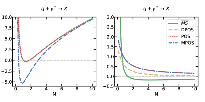
Figure 1: Mellin-space NLO contributions to deep-inelastic coefficient functions. The quark (left) and gluon (right) coefficient functions, respectively $C_{q}^{(1)}$ and $C_{g}^{(1)}$, Eq. 11, are shown. The DPOS scheme is defined in Eqs. (20,28), the POS scheme is defined in Eqs. (34-36), and the MPOS scheme in Eqs. (80-81). Results are shown in the $\overline{\rm{MS}}$ and DPOS, POS and MPOS schemes. For $C_{q}^{(1)}$ $\overline{\rm{MS}}$, DPOS and POS coincide, and the two curves shown correspond, from top to bottom, to $\overline{\rm{MS}}$ and MPOS; for $C_{g}^{(1)}$ POS and MPOS coincide and the three curves correspond, from bottom to top, to $\overline{\rm{MS}}$, DPOS and POS.

The $\overline{\rm{MS}}$ NLO contributions to the coefficient functions $C_{q}$ and $C_{g}$ are shown in Fig. 1 in Mellin space, where the convolution becomes an ordinary product. The Mellin space plot is especially transparent since the $x$-space cross section is found to high accuracy by computing the inverse Mellin transform in the saddle-point approximation [11]: hence, the physical $x$-space cross section is just the product of the Mellin-space coefficient function and PDF evaluated at the value of $N$ corresponding to the saddle for given kinematics. It is clear from Fig. 1 that at large $N$ the gluon coefficient function is negative on the real axis: hence, the $x$-space coefficient function must also be negative because its real moments are negative. This shows that a negative contribution has been factored from the coefficient function into the PDF.

2.1.1 Over-subtraction and the off-diagonal coefficient function

In order to understand what is going on, we look at the dimensionally regularized, unsubtracted gluon coefficient function:

$$C^{(1)}_{g}(z,Q^{2},\epsilon)=\frac{\Gamma(-\epsilon)\left(\frac{\mu_{D}^{2}}{\pi\mu^{2}}\right)^{-\epsilon}\left[8P_{qg}(z)-16T_{R}\epsilon(3-\epsilon(2-\epsilon))\right]}{16\pi(2-2\epsilon)\Gamma(3-2\epsilon)}\,,$$ (12)

where

$$\mu_{D}^{2}=\frac{s}{4}=\frac{Q^{2}(1-z)}{4z},$$ (13)

and $s=\frac{Q^{2}(1-z)}{z}$ is the center-of-mass energy of the $\gamma^{*}q$ collision. Note that in order to regulate the collinear singularity it is necessary to choose $\epsilon<0$; it then follows that as $\epsilon$ goes to zero from below, $\Gamma(-\epsilon)>0$ and the unsubtracted coefficient function, Eq. (12), is positive as it ought to be.

The subtracted $\overline{\rm{MS}}$ coefficient function is then given by

$${C^{(1)}_{g}}^{{\overline{\rm{MS}}}}(z) =\lim_{\epsilon\to 0^{-}}\left[C_{g}^{(1)}(z,Q^{2},\epsilon)-\left(\frac{Q^{2}}{4\pi\mu^{2}}\right)^{-\epsilon}\left(-\frac{1}{\epsilon}+\gamma_{E}\right)P_{qg}(z)\right]$$ (14)

$$=P_{qg}(z)\left(\ln\left(\frac{1-z}{z}\right)-4\right)+3T_{R}\,,$$ (15)

where $\epsilon\to 0^{-}$ denotes the fact that the limit should be taken from below, because the collinear singularity is regulated with $\epsilon<0$. The $P_{qg}$ splitting function is positive for all $z$, so for $z>\frac{1}{2}$ the log becomes negative and at large $z$ the coefficient function is negative.

Comparing Eqs. (12-14) immediately reveals what happened: the regularized coefficient function contains a term

$$\left(\frac{s/4}{\pi\mu^{2}}\right)^{-\epsilon}=1-\epsilon\ln\left(\frac{Q^{2}(1-z)/z}{4\pi\mu^{2}}\right),$$ (16)

but in the collinear subtraction $\ln\frac{Q^{2}}{4\pi\mu^{2}}$ has been subtracted instead. For $z>\frac{1}{2}$, $s<Q^{2}$ this amounts to over-subtracting, at the larger scale $Q^{2}$ instead of the smaller physical scale $s$. The physical origin of this contribution, and the reason for the mismatch are easy to trace.

Namely, this is the contribution coming from quark emission from the incoming gluon line, and the singularity is due to the collinear singular integration over the transverse momentum of the emitted quark, as revealed by the fact that it is proportional to the corresponding $P_{qg}$ splitting function. The argument of the ensuing collinear log is set by the upper limit of the transverse momentum integration $k_{T}^{\rm max}$, which for a $2\to 2$ process with massless particles in the final state is $k_{T}^{\rm max}=\frac{s}{4}$. In $\overline{\rm{MS}}$ the collinear subtraction is performed at the scale $Q^{2}$, hence leading to the over-subtraction that we observed, and producing a contribution to the coefficient function which is logarithmically enhanced in the threshold $z\to 1$ limit.

Therefore, this contribution has the same origin as the soft (Sudakov) logarithms which are resummed to all orders when performing threshold resummation [12, 13], except that in soft resummation the splitting function is evaluated in the $z\to 1$ limit, and the factor of $\frac{1}{z}$ in the argument of the log is neglected. In fact, threshold resummation can be obtained by identifying (and then renormalization-group improving)

$$|k_{T}^{\rm max,\,DIS}|^{2}=\mu_{D}^{2}$$ (17)

(with $\mu_{D}^{2}$ given by Eq. (13)) as the physical scale in the soft limit [14]. The over-subtraction is then simply the manifestation of the well-known fact that, in the $\overline{\rm{MS}}$ scheme, threshold logs beyond the first are factored in the coefficient function, and not in the PDF [15]. Indeed, alternative factorization schemes in which these logs are instead included in the PDF have been proposed, in particular the Monte Carlo factorization scheme of Ref. [16]. Note, however, that radiation in off-diagonal parton channels is power-suppressed in the threshold limit, and indeed this contribution is proportional to $\ln(1-z)$, which in Mellin space behaves as $\frac{\ln N}{N}$. This is to be contrasted with the $\left(\frac{\ln(1-z)}{1-z}\right)_{+}$ behavior, corresponding to $\ln^{2}N$, found in diagonal channels, as we shall discuss in Sect. 2.1.2 below. Hence, while it has the same origin, this contribution is not among those included in standard leading-power threshold resummation.

In conclusion, in order to restore positivity it is sufficient to perform the collinear subtraction at the scale $\mu_{D}^{2}=s/4$, Eq. (17). There is a further subtlety, however. Namely, the factor $2-2\epsilon$ in the denominator of Eq. (12) is the average over the polarization states of the incoming gluon. Therefore, it should be viewed as an overall prefactor which is common to both the unsubtracted and subtracted coefficient function, and thus must be included in the subtraction term. Because it interferes with a $-\frac{1}{\epsilon}$ pole, not including it, as in $\overline{\rm{MS}}$, leads to over-subtraction: the collinear singularity is regulated with $\epsilon<0$, so $\frac{1}{1-\epsilon}<1$.

Therefore, we define a modified positivity subtraction as

$${C^{(1)}_{g}}^{\rm DPOS}(z) =\lim_{\epsilon\to 0^{-}}\left[{C^{(1)}_{g}}(z,Q^{2},\epsilon)-\frac{1}{1-\epsilon}\left(\frac{\mu_{D}^{2}}{\pi\mu^{2}}\right)^{-\epsilon}\left(-\frac{1}{\epsilon}+\gamma_{E}\right)P_{qg}(z)\right]$$ (18)

$$=3\left[T_{R}-P_{qg}(z)\right].$$ (19)

Note that the normalization of the prefactor is fixed by the requirement of cancellation of the pole. The coefficient function of Eq. (18) is positive definite, as it is easy to check explicitly. Its Mellin-space form is also shown in Fig. 1, and it is manifestly positive.

We can rewrite the subtraction which relates the regularized coefficient function, Eq. (12), to its renormalized counterparts Eqs. (14,18) in terms of counterterms according to Eq. (10), where now $S={\overline{\rm{MS}}}$, DPOS. We then have

$${C^{(1)}_{g}}^{\rm DPOS}(z)={C^{(1)}_{g}}^{{\overline{\rm{MS}}}}(z)-K_{qg}^{\rm DPOS}(z)\,,$$ (20)

$$K_{qg}^{\rm DPOS}(z)=\delta_{qg}^{{\overline{\rm{MS}}}}-\delta_{qg}^{\rm DPOS}=P_{qg}(z)\left[\ln\left(\frac{1-z}{z}\right)-1\right].$$ (21)

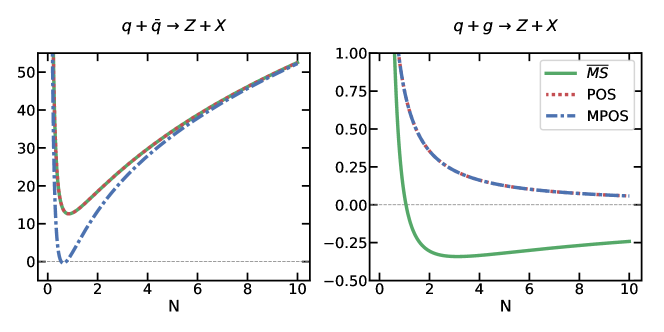
Figure 2: Mellin-space NLO contributions to Drell–Yan coefficient functions. The quark (left) and gluon (right) coefficient functions, respectively ${{{C^{q}}_{q}}^{(1)}}$ and ${{{C^{q}}_{g}}^{(1)}}$, Eq. (29), are shown. Results are shown in the $\overline{\rm{MS}}$, POS and MPOS schemes. The POS scheme is defined in Eqs. (34-36) and (44-46), and the MPOS scheme in Eqs. (80-83). ${{{C^{q}}_{q}}^{(1)}}$ $\overline{\rm{MS}}$ and POS coincide, and the two curves correspond, from top to bottom, to $\overline{\rm{MS}}$ and MPOS; for ${{{C^{q}}_{g}}^{(1)}}$ POS and MPOS coincide and the two curves correspond, from top to bottom, to $\overline{\rm{MS}}$ and POS.

2.1.2 The diagonal coefficient function

We now turn to the diagonal coefficient function: in the $\overline{\rm{MS}}$ scheme it is given by

$$C_{q}^{{\overline{\rm{MS}}}}(z) =\delta(1-z)+\frac{\alpha_{s}}{2\pi}{C^{(1)}_{q}}^{{\overline{\rm{MS}}}}(z)$$ (22)

$$=\delta(1-z)\left(1+\frac{\alpha_{s}}{2\pi}{\Delta^{(1)}_{q}}^{{\overline{\rm{MS}}}}\right)+\frac{\alpha_{s}}{2\pi}{\overline{C_{q}}^{(1)}}^{{\overline{\rm{MS}}}}(z)\,,$$ (23)

where in the last step we have separated off the contribution to ${C^{(1)}_{q}}^{{\overline{\rm{MS}}}}(z)$ proportional to a Dirac $\delta$ (corresponding to a constant in Mellin space) so that ${\overline{C_{q}}^{(1)}}^{{\overline{\rm{MS}}}}(z)$ only contains functions and $+$ distributions. The NLO diagonal coefficient function is given by

$${C^{(1)}_{q}}^{{\overline{\rm{MS}}}}(z) =\lim_{\epsilon\to 0^{-}}\left[C_{q}^{(1)}(z,Q^{2},\epsilon)-\left(\frac{Q^{2}}{4\pi\mu^{2}}\right)^{-\epsilon}\left(-\frac{1}{\epsilon}+\gamma_{E}\right)P_{qq}(z)\right]$$ (24)

$$=\lim_{\epsilon\to 0^{-}}\left[{C_{q}^{(1)}}(z,Q^{2},\epsilon)-\delta_{qq}^{{\overline{\rm{MS}}}}(z,Q^{2},\epsilon)\right]$$ (25)

$$=C_{F}\left[\left(p_{qq}(z)\ln\left(\frac{1-z}{z}\right)\right)_{+}-\frac{3}{2}{\left(\frac{1}{1-z}\right)_{+}}+3+2z-4\delta(1-z)\right],$$ (26)

where $p_{qq}(z)$ is implicitly defined in terms of the quark-quark splitting function $P_{qq}(z)$ as

$$P_{qq}(z)=C_{F}\left(p_{qq}(z)\right)_{+}.$$ (27)

The Mellin transform of $C^{(1)}_{q}(z)$ is shown in Fig. 1. It is clear that the coefficient function is positive for all $N$: the slightly negative dip of the NLO term in the $N\sim 1$ region is more than compensated by the much larger LO contribution, which in $N$ space is a constant (at $\frac{2\pi}{\alpha_{s}}$ on the scale of Fig. 1). As $N\to\infty$, where the NLO contribution diverges (and in principle needs resummation) the growth is actually positive.

A comparison of Eq. (26) with its off-diagonal counterpart, Eq. (15), immediately shows what is going on. In this case too, the $\overline{\rm{MS}}$ subtraction amounts to an over-subtraction, and indeed the term proportional to $p_{qq}(z)$ in the coefficient function Eq. (26) has the same origin as the term Eq. (16), namely, the collinear singularity due to real emission, in this case of a gluon from the incoming quark line. In fact, this is the contribution which is included in standard leading-log threshold resummation. Amusingly, the further (process-dependent) term, proportional to ${\left(\frac{1}{1-z}\right)_{+}}$, arises at the next-to-leading log level due to collinear radiation from the outgoing quark line [12], and thus has the same kinematic origin [14]. One may thus think of generally including these contributions in the PDF by changing the collinear subtraction, as we did above: indeed this is done in the Monte Carlo scheme of Ref. [16], which aims at including in PDFs all contributions coming from soft radiation.

However, if the goal is ensure positivity, in the diagonal case it is not necessary to modify the $\overline{\rm{MS}}$ subtraction prescription. Indeed, in this case over-subtraction actually leads to a more positive coefficient function, due to the fact that the $P_{qq}$ splitting function is negative at large $z$, where it reduces to a $+$ distribution, i.e., it leads to a negative answer when folded with a positive test function. Of course, this follows from baryon number conservation which requires the vanishing of the first moment of the splitting function. It is in fact easy to check that the $\overline{\rm{MS}}$ coefficient function, Eq. (22), is positive for all $z<1$. The term proportional to a $\delta$ of course has a positive coefficient in the perturbative regime, where it is dominated by the LO term.

We conclude that in order to ensure positivity of the coefficient function it is sufficient to modify the collinear subtraction only in the off-diagonal channel. We therefore set

$${C_{q}^{(1)}}^{\rm DPOS}(z)={C_{q}^{(1)}}^{{\overline{\rm{MS}}}}(z)\,.$$ (28)

Equations (20,28) thus define the DPOS factorization scheme in the quark channel, in terms of the $\overline{\rm{MS}}$ scheme. Note that the considerations underlying the construction of this factorization scheme are based on the structure of the collinear subtraction and the behavior of the splitting functions, and are therefore process-independent.

In order to fully characterize the scheme it is necessary to also consider gluon-induced processes. In Ref. [1], this was done by considering Higgs production in gluon fusion, with one of the two gluons coming from a proton and the other being taken as a pointlike probe. Equivalently, one might consider Higgs production in photon-gluon fusion. However, the treatment of these processes is essentially the same as that of hadronic processes, to which we thus turn.

2.2 Hadronic processes

For hadronic processes the basic factorization formula has the same structure as Eq. (11), with the structure function replaced by a cross section and the PDF replaced by a parton luminosity ${\cal L}_{ij}$: up to NLO

$$\frac{1}{x}\sigma(x,Q^{2})=\hat{\sigma}_{0}\left[{\cal L}_{ii}+\frac{\alpha_{s}}{2\pi}\left({{C^{i}}_{q}}^{(1)}\otimes{\cal L}_{iq}+{{C^{i}}_{g}}^{(1)}\otimes{\cal L}_{ig}\right)\right],$$ (29)

where for simplicity we consider process for which at LO only one partonic channel contributes, so $i=q,g$ labels quark-induced processes (such as Drell–Yan) or gluon-induced processes (such as Higgs production in gluon fusion), $\hat{\sigma}_{0}$ is the LO partonic cross section and the parton luminosity is

$${\cal L}_{ij}=f_{i}\otimes f_{j}\,.$$ (30)

We first discuss quark-induced processes: their treatment is very close to that of DIS presented in the previous section, so it is sufficient to highlight the differences. We then turn to gluon-induced processes, for which we repeat the analysis of Sect. 2.1.

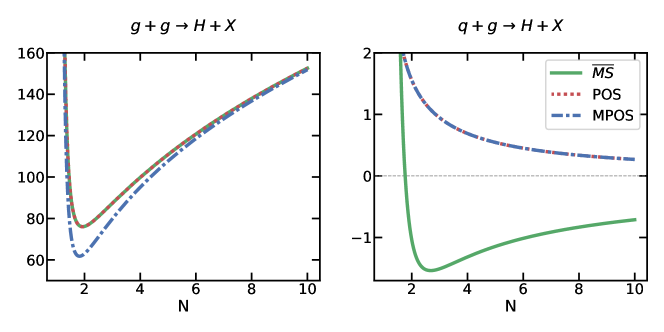
Figure 3: Same as Fig. 2, but now for the Higgs coefficient functions ${{{C^{g}}_{g}}^{(1)}}$ (left) and ${{{C^{g}}_{q}}^{(1)}}$ (right).

2.2.1 Quark-induced processes

As a prototype of quark-induced process we consider Drell–Yan production. The NLO coefficient functions (i.e. NLO partonic cross sections normalized to the LO result) are given by

$${{C^{q}{}_{q}}^{(1)}}^{{\overline{\rm{MS}}}}(z) =C_{F}\left[\left(\frac{4\pi^{2}}{3}-\frac{7}{2}\right)\delta(1-z)+2\left(p_{qq}(z)\ln\left(\frac{(1-z)^{2}}{z}\right)\right)_{+}\right]$$

$$={\Delta_{qq}^{(1)}}^{{\overline{\rm{MS}}}}\delta(1-z)+2C_{F}\left(p_{qq}(z)\ln\left(\frac{(1-z)^{2}}{z}\right)\right)_{+},$$ (31)

$${{C^{q}{}_{g}}^{(1)}}^{{\overline{\rm{MS}}}}(z) =P_{qg}(z)\left[\ln\left(\frac{(1-z)^{2}}{z}\right)-1\right]+C_{F}\left[\frac{3}{2}-\frac{3}{2}z^{2}+z\right].$$ (32)

Comparing the coefficient functions Eq. (2.2.1-32) to their DIS counterparts Eqs. (14,26) shows that they have the same structure, with a residual logarithmic contribution proportional to the splitting function, due to over-subtraction. The only difference is that the argument of the log is now $\frac{(1-z)^{2}}{z}$. This is again recognized to be the upper limit of the transverse momentum integral, and to coincide with the argument of the logs whose renormalization-group improvement leads to threshold resummation [14]: indeed, for a $2\to 2$ process with a final state particle with mass $M^{2}$, and $z=\frac{M^{2}}{s}$,

$$\mu_{h}^{2}=|k_{T}^{\rm max,\,had}|^{2}=\frac{(s-Q^{2})^{2}}{4s}=\frac{Q^{2}(1-z)^{2}}{4z}\,,$$ (33)

where $Q^{2}=M^{2}$. The coefficient functions, Eq. (2.2.1-32), are displayed in Fig. 2 in Mellin space; their qualitative features are the same as those of the DIS coefficient functions.

Hence, just as in case of DIS, it is possible to define a positive subtraction scheme, which we call POS, and which differs from $\overline{\rm{MS}}$ because in the off-diagonal quark-gluon channel the subtraction is performed at the scale $\mu_{h}^{2}$, Eq. (33). Just like for DIS, in the diagonal quark-quark channel there is no need to modify the $\overline{\rm{MS}}$ subtraction, which actually makes the coefficient function more positive, so we define a POS factorization of the DY process according to

$${{C^{q}{}_{q}}^{(1)}}^{\rm POS}(z) ={{C^{q}{}_{q}}^{(1)}}^{{\overline{\rm{MS}}}}(z)\,,$$ (34)

$${{C^{q}{}_{g}}^{(1)}}^{\rm POS}(z) ={{C^{q}{}_{g}}^{(1)}}^{{\overline{\rm{MS}}}}(z)-K_{qg}^{\rm POS}(z)\,,$$ (35)

$$K_{qg}^{\rm POS}(z) =P_{qg}(z)\left[\ln\left(\frac{(1-z)^{2}}{z}\right)-1\right]\,.$$ (36)

The quark-gluon coefficient function can be read off Eqs. (32,36) and it is easy to check that it is positive definite for all $0<z<1$.

Of course, a choice of factorization scheme must be universal. Therefore, it is interesting to check what this choice amounts to if adopted for DIS. Clearly, the hadronic scale Eq. (33) is always lower than the DIS scale Eq. (33): $\mu_{h}^{2}<\mu_{D}^{2}$. Hence, subtraction in the DPOS scheme amounts to under-subtraction, and if adopted for DIS coefficient function it leads to a DIS coefficient function ${C^{(1)}_{g}}^{\rm POS}(z)$ which is actually more positive than that in the DPOS scheme. This is seen in Fig. 1 (right), where ${C^{(1)}_{g}}(z)$ is shown in the $\overline{\rm{MS}}$, DPOS and POS schemes.

2.2.2 Gluon-induced processes

In order to fix completely the factorization scheme we turn to gluon-induced hadronic processes. We choose Higgs production in gluon fusion (in the infinite top mass limit) as a prototype, and we repeat the analysis of Sect. 2.1.1, but now for the quark coefficient function ${{{C^{g}}_{q}}^{(1)}}$. The regularized, unsubtracted expression is (see e.g. [17])

$${C^{g}{}_{q}}^{(1)}(z,Q^{2},\epsilon)=\frac{\Gamma(-\epsilon)\left(\frac{\mu_{h}^{2}}{\pi\mu^{2}}\right)^{-\epsilon}(1-\epsilon)\left[P_{gq}(z)-C_{F}\frac{(1+z)^{2}}{2z}\epsilon\right]}{16\pi(2-2\epsilon)\Gamma(3-2\epsilon)}\,,$$ (37)

where $\mu_{h}^{2}$ is given by Eq. (33), with $Q^{2}=M_{H}^{2}$, the Higgs square mass. Performing $\overline{\rm{MS}}$ subtraction in the usual way we get

$${{C^{g}{}_{q}}^{(1)}}^{{\overline{\rm{MS}}}}(z) =\lim_{\epsilon\to 0^{-}}\left[{{C^{g}}_{q}}^{(1)}(z,Q^{2},\epsilon)-\left(\frac{Q^{2}}{4\pi\mu^{2}}\right)^{-\epsilon}\left(-\frac{1}{\epsilon}+\gamma_{E}\right)P_{gq}(z)\right]$$ (38)

$$=P_{gq}(z)\left[\ln\left(\frac{(1-z)^{2}}{z}\right)-1\right]+C_{F}\frac{(1+z)^{2}}{2z}\,.$$ (39)

Again, we encounter the same situation that we have seen in the quark channel for DIS, Eqs. (12,14): the collinear log has a scale set by the upper limit of the transverse momentum integration, now the hadronic $\mu_{h}^{2}$, Eq. (33), but the $\overline{\rm{MS}}$ subtraction is performed at the scale $Q^{2}$, which at large $z$ is higher, thus leading to over-subtraction. Indeed, the Mellin-space $\overline{\rm{MS}}$ coefficient function ${{{C^{g}}_{q}}^{(1)}}$, shown in Fig. 3, is seen to be negative at large $N$.

As in the quark sector, the problem is fixed by performing the collinear subtraction at the physical scale $\mu_{h}^{2}$. Note that also in this case, as for the DIS quark-gluon channel, there is an issue with the sum over gluon polarizations: indeed, because the LO process is in the gluon-gluon channel, even the NLO quark-gluon channel has a gluon in the initial state, leading to a factor $1-\epsilon$ in the denominator of Eq. (37), which must be accounted for in order to avoid over-subtraction. Hence, we define the POS scheme coefficient function as

$${{C^{g}{}_{q}}^{(1)}}^{\rm POS}(z) =\lim_{\epsilon\to 0^{-}}\left[{C^{g}{}_{q}}^{(1)}(z,Q^{2},\epsilon)-\frac{1}{1-\epsilon}\left(\frac{\mu_{h}^{2}}{\pi\mu^{2}}\right)^{-\epsilon}\left(-\frac{1}{\epsilon}+\gamma_{E}\right)P_{qg}(z)\right]$$ (40)

$$=C_{F}\frac{(1+z)^{2}}{2z}\,,$$ (41)

with $\mu_{h}^{2}$ given by Eq. (33). The coefficient function is clearly positive. Its Mellin transform is also shown in Fig. 3.

We finally examine the gluon-gluon NLO coefficient function:

$${{C^{g}{}_{g}}^{(1)}}^{{\overline{\rm{MS}}}}(z) =C_{A}\left[2\frac{1}{z}\left(zp_{gg}(z)\ln\left(\frac{(1-z)^{2}}{z}\right)\right)_{+}+\left(\frac{473}{36}+\frac{4\pi^{2}}{3}\right)\delta(1-z)-\frac{11}{3}\frac{(1-z)^{3}}{z}\right]$$

$$={\Delta^{(1)}_{gg}}^{{\overline{\rm{MS}}}}\delta(1-z)+C_{A}\left[2\frac{1}{z}\left(zp_{gg}(z)\ln\left(\frac{(1-z)^{2}}{z}\right)\right)_{+}-\frac{11}{3}\frac{(1-z)^{3}}{z}\right]\,,$$ (42)

where, in analogy to Eq. (27), $p_{gg}(x)$ is implicitly defined by

$$P_{gg}(z)=C_{A}\frac{1}{z}\left(zp_{gg}(z)\right)_{+}-\frac{n_{f}}{3}\delta(1-z).$$ (43)

As in the diagonal quark channel, the $\overline{\rm{MS}}$ subtraction is now multiplied by a splitting function which is negative at large $z$, for the same physical reason. It therefore leads to a coefficient function which is positive, as seen by inspecting Eq. (2.2.2) and shown in Fig. 3 (left), so no further scheme change is needed.

Therefore we get

$${{C^{g}{}_{g}}^{(1)}}^{\rm POS}(z) ={{C^{g}{}_{g}}^{(1)}}^{{\overline{\rm{MS}}}}(z)\,,$$ (44)

$${{C^{g}{}_{q}}^{(1)}}^{\rm POS}(z) ={{C^{q}{}_{g}}^{(1)}}^{{\overline{\rm{MS}}}}(z)-K_{gq}^{\rm POS}(z)\,,$$ (45)

$$K_{gq}^{\rm POS}(z) =P_{gq}(z)\left[\ln\left(\frac{(1-z)^{2}}{z}\right)-1\right].$$ (46)

Equations (34-36) and (44-46) fully define the POS subtraction. We shall see in the next section that they define a positive factorization scheme. Indeed, in the construction presented in this section we have not made use of the detailed from of the partonic cross section, but rather just of the collinear counterterms, expressed in terms of universal splitting functions. Hence, these counterterms, when used in Eq. (4) define a universal renormalization scheme Eq. (3) for PDFs, without spoiling PDF universality.

3 A positive factorization scheme

We will now construct a positive factorization scheme based on the POS subtraction of Eqs. (34-36,44-46). We then discuss the scheme transformation from this scheme to the $\overline{\rm{MS}}$ scheme and use it to show that PDFs are non-negative in the $\overline{\rm{MS}}$ scheme in the perturbative region.

The argument is based on the factorization Eqs. (6-7), and, very crudely speaking, amounts to showing that with the POS subtraction, all factors in Eqs. (7) are positive: the left-hand side is positive because it is a physically measurable cross-section, the coefficient $C^{S}$ function on the right-hand side is positive because the POS subtraction preserves the positivity of the unsubtracted coefficient function $C$, which is a partonic cross-section, and thus positive before subtraction, but only well-defined in $d>4$ dimensions.

Taking a Mellin transform of both sides of Eqs. (6-7) all convolutions turn into ordinary products, and it is immediately clear that, because the left-hand side is positive, for the Mellin transformed PDF to be positive it is necessary and sufficient that the coefficient function is positive. However, positivity of the Mellin transform of a function is a necessary condition for its positivity, but not a sufficient one: a negative function may have a positive Mellin transform. The somewhat more complex structure of the discussion below is necessary in order to deal with the necessity of providing an $x$-space argument.

3.1 Positive PDFs

We start by presenting the construction in a simplified setting, namely in the absence of parton mixing. This means that the operators Eq. (2) whose matrix elements define the PDFs renormalize multiplicatively. This would specifically correspond to the case of a quark combination that does not mix with the gluon, such as any combination $q^{{\rm NS}}(Q^{2})=q_{i}(Q^{2})-q_{j}(Q^{2})$, where $i,\>j$ denote generically a quark flavor or antiflavor, with $i\not=j$. We refer to this as a nonsinglet quark combination. We can think of the argument below as applying to such a combination, chosen in such a way that the bare $q^{{\rm NS}}(Q^{2})^{(0)}$, Eq. (2), is positive — which in general of course will not be true even if $q_{i}$ and $q_{j}$ are separately positive. This should be viewed as an academic case — after all, in principle, a positive nonsinglet PDF might not exist — whose purpose is to illustrate the structure of the argument in the absence of parton mixing. We then turn to the realistic case of PDFs that do undergo mixing upon renormalization (which we will refer to as singlet case). The nonsinglet case is simpler, not only because of the absence of mixing, but also because in this case the POS scheme actually coincides with $\overline{\rm{MS}}$ (i.e., $\overline{\rm{MS}}$ is already positive).

3.1.1 The nonsinglet case as a toy model

In the nonsinglet case, only the diagonal quark subtraction is relevant: so in the nonsinglet case the DIS structure function Eq. (11) becomes

$$\frac{1}{x}F_{2}^{{\rm NS}}(x,Q^{2})=\langle e_{i}^{2}\rangle\left[1+\frac{\alpha_{s}}{2\pi}C^{(1)}_{q}\otimes\right]q^{{\rm NS}}(Q^{2})\,,$$ (47)

where $q^{{\rm NS}}$ is a difference of two quark or antiquark PDFs, assumed positive and $\langle e^{2}_{i}\rangle=\frac{1}{2}\left(e^{2}_{i}+e^{2}_{j}\right)$ is the average of their electric charges.

The factorization Eqs. (6-7) takes the form

$$\frac{1}{x}F_{2}^{{\rm NS}}(x,Q^{2}) =\langle e_{i}^{2}\rangle\lim_{\epsilon\to 0^{-}}\left[1+\frac{\alpha_{s}}{2\pi}C_{q}^{(1)}(Q^{2},\epsilon)\otimes\right]\left[{q^{{\rm NS}}}\right]^{(0)}$$ (48)

$$=\langle e_{i}^{2}\rangle\lim_{\epsilon\to 0^{-}}\left[1+\frac{\alpha_{s}}{2\pi}{C_{q}^{(1)}}^{{\overline{\rm{MS}}}}(Q^{2},\epsilon)\otimes\right]\left[1+\frac{\alpha_{s}}{2\pi}\delta^{{\overline{\rm{MS}}}}(Q^{2},\epsilon)\otimes\right]\left[{q^{{\rm NS}}}\right]^{(0)}$$ (49)

$$=\langle e_{i}^{2}\rangle\left[1+\frac{\alpha_{s}}{2\pi}{\Delta^{(1)}_{q}}^{{\overline{\rm{MS}}}}+\frac{\alpha_{s}}{2\pi}{\bar{C}_{q}^{(1)}{}}^{{\overline{\rm{MS}}}}\otimes\right]\left[{q^{{\rm NS}}}\right]^{{\overline{\rm{MS}}}}(Q^{2})\,,$$ (50)

where ${C_{q}^{(1)}}^{{\overline{\rm{MS}}}}$, ${\overline{C_{q}}^{(1)}}^{{\overline{\rm{MS}}}}$, ${\Delta^{(1)}_{q}}^{{\overline{\rm{MS}}}}$ and $\delta_{qq}^{{\overline{\rm{MS}}}}$ have been defined in Eqs. (23,24,25), and the dependence on $x$ on the right-hand side has been omitted because it appears due to the convolution, while the dependence on all other variables has been indicated explicitly.

Now, the discussion of Sect. 2.1 shows that, because the bare PDF of Eq. (2) is a probability density, the three factors which are convoluted in Eq. (50) are all separately positive when $\epsilon\to 0^{-}$, i.e. from the negative region, provided only $\mu^{2}<\mu_{D}^{2}$, with $\mu_{D}^{2}$ given by Eq. (13). This, as discussed in Sect. 2.1.2 [see in particular Eq. (26) and Fig. 1] can be understood as a consequence of the fact that the only region in which the $O(\alpha_{s})$ term could overwhelm the LO contribution is the threshold region $z\to 1$, where $\alpha_{s}\ln(1-z)\sim 1$. However, in this region the $\overline{\rm{MS}}$ over-subtraction leads to a coefficient function which is positive because $P_{qq}$ is negative at large $z$. Consequently, all factors in Eq. (50) remain positive for all $z$.

The meaning of the factorization argument Eqs. (48-50) can be understood by noting that it is possible to choose a “physical” factorization scheme [18] in which PDFs are identified with physical observables. This means that the coefficient function is set to one to all orders by scheme choice. An example is the “DIS” scheme [19] in which the quark PDF is identified with the DIS structure function, so that Eq. 47 becomes

$$\frac{1}{x}F_{2}^{{\rm NS}}(x,Q^{2})=\langle e_{i}^{2}\rangle\left[{q^{{\rm NS}}}\right]^{\rm DIS}(x,Q^{2})\,,$$ (51)

which holds to all perturbative orders. Comparing this DIS scheme expression of the structure function to the $\overline{\rm{MS}}$ expression, Eq. (11), immediately shows that the quark PDF in the DIS and $\overline{\rm{MS}}$ schemes are related by

$$\left[{q^{{\rm NS}}}\right]^{\rm DIS}(\xi,Q^{2})=\left[1+\frac{\alpha_{s}}{2\pi}{\Delta^{(1)}_{q}}^{{\overline{\rm{MS}}}}+\frac{\alpha_{s}}{2\pi}{{{\bar{C}}^{(1)}}_{q}{}}^{{\overline{\rm{MS}}}}\otimes\right]\left[{q^{{\rm NS}}}\right]^{{\overline{\rm{MS}}}}(Q^{2})\,,$$ (52)

where again we have dropped the $\xi$ dependence of the convolution on the right-hand side, as in Eqs. (48-50).

The $\overline{\rm{MS}}$ PDFs can be obtained in terms of the DIS ones by inverting Eq. (52): perturbative inversion of course gives

$$\left[{q^{{\rm NS}}}\right]^{{\overline{\rm{MS}}}}(\xi,Q^{2})=\left[1-\frac{\alpha_{s}}{2\pi}{\Delta^{(1)}_{q}}^{{\overline{\rm{MS}}}}-\frac{\alpha_{s}}{2\pi}{\bar{C}^{(1)}_{q}{}}^{{\overline{\rm{MS}}}}\otimes\right]\left[{q^{{\rm NS}}}\right]^{\rm DIS}(Q^{2})+O(\alpha_{s}^{2})\,.$$ (53)

One may worry that therefore the $\overline{\rm{MS}}$ PDFs may turn negative in the large $\xi$ region, where $\alpha_{s}\ln(1-\xi)\gtrsim 1$ and the last term in square brackets in Eq. (53), which is negative, may overwhelm the LO contribution term. However, in this region the perturbative inversion is invalid, but it is easy to invert Eq. (52) exactly in the asymptotic large $\xi$ limit. Letting

$$\left[{q^{{\rm NS}}}\right]^{\rm DIS}(\xi,Q^{2}) =\left[1+\frac{\alpha_{s}}{2\pi}{\Delta^{(1)}_{q}}^{{\overline{\rm{MS}}}}+\frac{\alpha_{s}}{2\pi}2C_{F}\left[\frac{\ln(1-z)}{1-z}\right]_{+}\otimes\right]\left[{q^{{\rm NS}}}\right]^{{\overline{\rm{MS}}}}(Q^{2})$$

$$\qquad+\hbox{NLL}(1-\xi)$$ (54)

$$=\left(1+\frac{\alpha_{s}}{2\pi}{\Delta^{(1)}_{q}}^{{\overline{\rm{MS}}}}\right)\left[1+c_{\rm LL}\left[\frac{\ln(1-z)}{1-z}\right]_{+}\otimes\right]\left[{q^{{\rm NS}}}\right]^{{\overline{\rm{MS}}}}(Q^{2})$$

$$\qquad+\hbox{NLL}(1-\xi)\,,$$ (55)

with

$$c_{\rm LL}=\frac{\frac{\alpha_{s}}{2\pi}2C_{F}}{1+\frac{\alpha_{s}}{2\pi}{\Delta^{(1)}_{q}}^{{\overline{\rm{MS}}}}}\,,$$ (56)

and which holds at the leading $\ln(1-\xi)$ level (LL$(1-\xi)$), inversion can be performed by going to Mellin space and then computing the Mellin inverse term by term in an expansion in powers of $\alpha_{s}$. We get

$$\left[{q^{{\rm NS}}}\right]^{{\overline{\rm{MS}}}}(\xi,Q^{2}) =\frac{1}{1+\frac{\alpha_{s}}{2\pi}{\Delta^{(1)}_{q}}^{{\overline{\rm{MS}}}}}\times$$

$$\Bigg{[}1-c_{\rm LL}\left[\frac{\ln(1-z)}{\left[1+c_{\rm LL}\ln^{2}(1-z)/2\right]^{2}}\frac{1}{1-z}\right]_{+}\otimes\Bigg{]}\left[{q^{{\rm NS}}}\right]^{\rm DIS}(Q^{2})+\hbox{NLL}(1-\xi)\,.$$ (57)

It is clear that as $\xi\to 1$ the negative LL$(1-\xi)$ contribution actually vanishes.

Now, we observe that $\left[{q^{{\rm NS}}}\right]^{\rm DIS}(\xi,Q^{2})$ is positive because it is a physical observable. Equation (52), which expresses the DIS PDF in terms of the $\overline{\rm{MS}}$ one, then implies that for $\left[{q^{{\rm NS}}}\right]^{{\overline{\rm{MS}}}}(\xi,Q^{2})$ to be guaranteed to be positive, the $\overline{\rm{MS}}$ coefficient function must also be positive, otherwise folding a positive $\overline{\rm{MS}}$ PDF with a negative coefficient function could lead to a negative DIS PDF. So positivity of the $\overline{\rm{MS}}$ coefficient function is a necessary condition for positivity of the $\overline{\rm{MS}}$ PDF. However, the inverse of Eq. (52), expressing the $\overline{\rm{MS}}$ PDF in terms of the DIS one, implies that the condition is also sufficient, because it gives the $\overline{\rm{MS}}$ PDF as the convolution of a positive coefficient with a positive PDF. Equations. (53,3.1.1) show that the coefficient is indeed positive because in the dangerous $\xi\to 1$ region, where a large negative contribution may arise, inversion can be performed exactly and shown to lead to a positive result. Of course, this argument works for any factorization scheme, and it shows that a necessary and (perturbatively) sufficient condition for the PDFs to be positive is that the coefficient function in that scheme is positive.

The perturbative nature of the argument is worth commenting upon. As discussed at the beginning of this section, the corresponding Mellin space argument is trivial: because in Mellin space the structure function is the product of the PDF times the coefficient function, it follows that positivity of the coefficient function is necessary and sufficient for the positivity of the PDF. However, as already mentioned, Mellin-space positivity is not sufficient for $x$-space positivity. It is therefore necessary to compute the $x$-space inverse of the coefficient function, and check that it is still positive.

The inversion is done perturbatively in Eq. (53), and it leads to a coefficient function which is manifestly positive in most of the $z$ range, except at small and large $z$, where the coefficient functions blows up, due to high-energy (BFKL) and soft (Sudakov) logs respectively. Consider the large-$z$ case that was discussed above. Upon Mellin transformation, the $z\to 1$ region is mapped onto the $N\to\infty$ region, and specifically, as well known (see e.g. Ref. [14]) powers of $\ln(1-z)$ are mapped onto powers of $\ln N$. The $\ln N$ logarithmic growth of the coefficient function in this limit is seen in Fig. 1, where it is apparent that the coefficient function diverges as $N\to\infty$. The $N$-space inverse of the coefficient function is just its reciprocal, and thus it manifestly vanishes as $N\to\infty$ (while of course remaining positive). One would therefore naively expect that the $x$-space inverse also vanishes (from the positive side) as $z\to 1$, and this expectation is borne out by the explicit computation presented above in Eq. (3.1.1). Similar arguments apply at higher orders (NNLO and beyond), where the coefficient function grows with a higher order power of $\ln(1-z)$ as $z\to 1$, and at small $z$, where the coefficient function grows as powers of $\ln\frac{1}{z}$ as $z\to 0$. Hence, either the coefficient function is not logarithmically enhanced, and then the perturbative inverse is manifestly positive, or it is logarithmically enhanced, and then the exact inverse of the enhanced terms can be computed ans also shown to be positive. It is natural to conjecture that an explicit computation of the exact inverse of the full coefficient function would also be positive.

The perturbative assumption is therefore used in two different ways. On the one hand, the NLO correction to the $\overline{\rm{MS}}$ coefficient function ${\bar{C}^{(1)}_{q}(z)}^{{\overline{\rm{MS}}}}$ is not everywhere positive, as it is apparent from Fig. 1. However, this is a small correction to the positive coefficient function if $\alpha_{s}\lesssim 1$, and the overall coefficient function remain positive. This would fail in a region in which $\alpha_{s}$ blows up. So the full NLO coefficient function remains positive, but only in the perturbative region. On the other hand, the perturbative inversion Eq. (53) is used to show that positivity of the coefficient function is shared by its inverse, and in regions in which perturbativity would fail it is checked explicitly that this is the case by exact inversion. In this case we conjecture that positivity of the inverse is actually an exact property, even when $\alpha_{s}$ is arbitrarily large.

The argument based on the physical factorization scheme showing that a positive coefficient function is necessary and (perturbatively) sufficient for a positive PDF is in fact equivalent to the factorization argument Eqs. (48-50). Indeed, the operator definition of the quark distribution, Eq. (2), upon performing a derivative expansion of the Wilson line, leads to the standard expression of its moments in terms of matrix elements of local operators. The interpretation of the bare quark distribution as a probability is then preserved by any physical subtraction scheme such that the matrix elements of Wilson operators are expressed in terms of a measurable quantity. The DIS scheme of Eq. (47) is of course an example of this scheme. Given the equivalence of the two arguments, one may wonder whether, if at all, perturbativity is used in the argument of Eqs. (48-50): specifically, the perturbative inversion of Eq. (53). The question is answered in the affirmative: the perturbative inversion is hidden in the step leading from Eq. (48) to Eq. (49). Indeed, this step amounts to

$$\left[1+\frac{\alpha_{s}}{2\pi}{C_{q}^{(1)}}^{{\overline{\rm{MS}}}}\otimes\right]^{-1}\left[1+\frac{\alpha_{s}}{2\pi}C_{q}^{(1)}(Q^{2},\epsilon)\right]=\left[1+\frac{\alpha_{s}}{2\pi}\delta^{{\overline{\rm{MS}}}}(Q^{2},\epsilon)\right]+O(\alpha_{s}^{2})\,,$$ (58)

i.e. the perturbative inversion of the $\overline{\rm{MS}}$ coefficient function. The two arguments are thus seen to coincide. Again, while we only provide a perturbative argument it is natural to conjecture that the argument is in fact exact (i.e. it also holds for large values of $\alpha_{s}$).

3.1.2 The POS factorization scheme

Equipped with the results of Sect. 3.1.1 we can turn to the case in which parton mixing is present. This corresponds to the realistic case in which the operators Eq. (2) mix with the gluon and conversely (at NLO) and with each other at NNLO and beyond. Because at NLO only quark-gluon mixing is present, we refer to this as the singlet case. In order to fully define the factorization scheme at NLO we must thus consider a pair of processes, a quark-induced and a gluon-induced one. The factorization for a pair of hadronic processes can be written as

$$\frac{1}{x}\sigma(x,Q^{2})=\hat{\Sigma}_{0}\otimes\left[1+\frac{\alpha_{s}}{2\pi}C^{(1)}\otimes\right]f(Q^{2})\,.$$ (59)

In Eq. (59)

• $\sigma(x,Q^{2})$ is a vector of hadronic cross sections

  $$\sigma(x,Q^{2})=\left(\begin{array}[]{c}\sigma^{q}(x,Q^{2})\\ \sigma^{g}(x,Q^{2})\end{array}\right),$$ (60)

  such as the pair of processes of Sect. 2.2, namely Drell–Yan and Higgs production in gluon fusion; we are assuming for simplicity and without loss of generality that both are evaluated at the same scale $Q^{2}=M^{2}$ (such as when producing an off-shell gauge boson and/or Higgs with the same mass), with a trivial generalization to the case of unequal scales, and the scaling variable is $x=\frac{Q^{2}}{s}$, with $s$ the hadronic center-of-mass energy;

• $\hat{\Sigma}_{0}$ is a diagonal matrix of LO partonic cross sections, multiplied by the respective PDFs,

  $$\hat{\Sigma}_{0}(x,Q^{2})=\left(\begin{array}[]{cc}\hat{\sigma}_{0}^{q}q(x,Q^{2})&0\\ 0&\sigma_{0}^{g}g(x,Q^{2})\end{array}\right),$$ (61)

  namely the quark and the gluon respectively for Drell–Yan and Higgs;

• $C^{(1)}$ is the two-by-two matrix of NLO coefficient functions ${C^{i}{}_{j}}^{(1)}$ with $i,\,j=q,\,g$ defined in Eq. (29);

• $f(\xi,Q^{2})$ is a vector of PDFs that mix upon renormalization:

  $$f(\xi,Q^{2})=\left(\begin{array}[]{c}q(\xi,Q^{2})\\ g(\xi,Q^{2})\end{array}\right).$$ (62)

Having established a suitable notation, the argument then proceeds in an analogous way as the nonsinglet argument of Sect. 3.1.1, except that now, in order to guarantee positivity of the two-by-two matrix of coefficient functions, we must perform the POS subtraction, which in the diagonal channels (and thus in the nonsinglet case) coincides with $\overline{\rm{MS}}$ but in the off-diagonal channel differs from it. Namely, we have

$$\frac{1}{x}\sigma(x,Q^{2}) =\hat{\Sigma}_{0}\otimes\lim_{\epsilon\to 0^{-}}\left[\mathbb{I}+\frac{\alpha_{s}}{2\pi}C^{(1)}(Q^{2},\epsilon)\otimes\right]f^{(0)}$$ (63)

$$=\hat{\Sigma}_{0}\otimes\lim_{\epsilon\to 0^{-}}\left[\mathbb{I}+\frac{\alpha_{s}}{2\pi}{C^{(1)}}^{{\rm POS}}(Q^{2},\epsilon)\otimes\right]\left[\mathbb{I}+\frac{\alpha_{s}}{2\pi}\delta^{{\rm POS}}(Q^{2},\epsilon)\otimes\right]f^{(0)}$$ (64)

$$=\hat{\Sigma}_{0}\otimes\left[\mathbb{I}+\frac{\alpha_{s}}{2\pi}{\Delta^{(1)}}^{{\rm POS}}+\frac{\alpha_{s}}{2\pi}{\overline{C}^{(1)}}^{{\rm POS}}\otimes\right]f^{{\rm POS}}(Q^{2})\,.$$ (65)

In Eqs. (63-65)

• ${\Delta^{(1)}}^{{\rm POS}}$ is the diagonal matrix

  $${\Delta^{(1)}}^{{\rm POS}}=\left(\begin{array}[]{cc}{\Delta_{qq}^{(1)}}^{{\overline{\rm{MS}}}}&0\\ 0&{\Delta_{gg}^{(1)}}^{{\overline{\rm{MS}}}}\end{array}\right),$$ (66)

  with ${\Delta_{ii}^{(1)}}^{{\overline{\rm{MS}}}}$ defined in Eqs. (2.2.1) and (2.2.2) respectively for $i=q$ and $i=g$;

• $\delta^{{\rm POS}}(Q^{2},\epsilon)$ is a two-by-two matrix of counterterms

  $$\delta^{{\rm POS}}(z,Q^{2},\epsilon)=\left(-\frac{1}{\epsilon}+\gamma_{E}\right)\left(\begin{array}[]{cc}\left(\frac{Q^{2}}{4\pi\mu^{2}}\right)^{-\epsilon}P_{qq}(z)&\frac{1}{1-\epsilon}\left(\frac{\mu_{h}^{2}}{\pi\mu^{2}}\right)^{-\epsilon}P_{qg}(z)\\ \frac{1}{1-\epsilon}\left(\frac{\mu_{h}^{2}}{\pi\mu^{2}}\right)^{-\epsilon}P_{gq}(z)&\left(\frac{Q^{2}}{4\pi\mu^{2}}\right)^{-\epsilon}P_{gg}(z)\end{array}\right),$$ (67)

  with $\mu_{h}^{2}$ given by Eq. (33), so that in the diagonal channels the subtraction is the same as in $\overline{\rm{MS}}$, while in the off-diagonal channels it is performed at the physical scale $\mu_{h}^{2}$, and also, accounting for the $d$-dimensional continuation of the average over the polarization of the gluons.

Positivity of the quark and gluon PDF vector $f^{{\rm POS}}(Q^{2})$, Eq. (65), now follows from the same argument used to show the positivity of the nonsinglet PDF Eq. (50). Namely, all factors, which are convoluted in Eq. (50), are separately positive when $\epsilon\to 0^{-}$ and $\mu_{h}^{2}<\mu_{D}^{2}$ (with $\mu_{D}$ defined in Eq. (13)) and in particular, the matrix of POS-scheme coefficient functions is now positive as shown in Sect. 2.2.

Also, as in the nonsinglet case, the positivity argument can be formulated in terms of a physical scheme, in which now to all perturbative orders the quark and gluon are defined by

$$\frac{1}{x}\bar{\sigma}(x,Q^{2})=f^{\rm PHYS}(x,Q^{2})\,,$$ (68)

where, as in Ref. [1], the hadronic cross sections $\bar{\sigma}(x,Q^{2})$ are computed assuming that one of the two incoming protons is replaced by a beam of antiquarks or a beam of gluons respectively, i.e.

$$\bar{\sigma}(x,Q^{2})=\left(\begin{array}[]{c}\sigma(x,Q^{2})[\bar{q}p\to\gamma^{*}+X]\\ \sigma(x,Q^{2})[gp\to H+X]\end{array}\right).$$ (69)

This hadronic cross section is linear in the PDFs, it coincides with it at LO in any scheme, and, assuming that it coincides with it to all orders, defines the PHYS scheme. Equivalently, one could choose as $\bar{\sigma}$ a DIS structure function in the quark channel, and the cross section for Higgs production in photon-gluon fusion in the gluon channel. The POS and PHYS schemes are then related by

$$f^{\rm PHYS}(x,Q^{2})=\left[\mathbb{I}+\frac{\alpha_{s}}{2\pi}{\Delta^{(1)}}^{\rm POS}+\frac{\alpha_{s}}{2\pi}{\bar{C}^{(1)}{}}^{\rm POS}\otimes\right]f^{\rm POS}(Q^{2})\,,$$ (70)

which is perturbatively inverted as

$$f^{\rm POS}(x,Q^{2})=\left[\mathbb{I}-\frac{\alpha_{s}}{2\pi}{\Delta^{(1)}}^{\rm POS}-\frac{\alpha_{s}}{2\pi}{\bar{C}^{(1)}{}}^{\rm POS}\otimes\right]f^{\rm PHYS}(Q^{2})+O(\alpha_{s}^{2})\,.$$ (71)

Again, this shows that positivity of the POS-scheme coefficient function is necessary for positivity of the POS-scheme PDFs and sufficient if perturbativity holds. Just like in the case of Eq. (53), this assumption fails at the endpoints $z\to 0$ and $z\to 1$. However, as well known [7], and as it is easy to check from the explicit expressions of the matrix elements of ${\bar{C}^{(1)}(z)}^{\rm POS}$, in both these limits the matrix is diagonal up to power-suppressed corrections. Specifically, in the $z\to 1$ limit the coefficient function matrix is diagonal:

$$\lim_{z\to 1}{C^{(1)}}^{\rm POS}(z,Q^{2})=\left(\begin{array}[]{cc}{{{C^{q}}_{q}}^{(1)}}^{\rm POS}&0\\ 0&{{{C^{g}}_{g}}^{(1)}}^{\rm POS}\end{array}\right)\left[1+O(1-z)\right].$$ (72)

Indeed, diagonal coefficient functions grow as $\left(\frac{\ln(1-z)}{(1-z)}\right)_{+}$ while off-diagonal ones tend to a constant as $z\to 1$. This is clearly seen in the $N$ space plots of Figs. 2-3, in which as $N\to\infty$ the diagonal coefficient functions are seen to grow (as $\ln^{2}N$) while the off-diagonal ones vanish (as $\frac{1}{N}$)  It follows that at large $z$ the quark and gluon channels decouple, and the perturbativity argument is the same as in the nonsinglet case.

3.1.3 Positive PDFs and their scale dependence

In Section 3.1.2 we have shown that also in the presence of quark-gluon mixing POS-scheme coefficient functions are positive, and thus in the perturbative regime PDFs are also positive. One can then ask two (closely related) questions. First, at which scale does this conclusion apply, and is it affected by perturbative evolution? And second, which PDF combinations are actually positive? Indeed, as well known, the eigenstates of QCD evolution are the two eigenstates of a mixing matrix between the quark singlet and the gluon, and individual nonsinglet components; any PDF (and thus any observable) can be decomposed into a singlet and nonsinglet component, which evolve independently (see e.g. Sect. 4.3.3 of Ref. [7]). Of course a difference between two positive quantities is not necessarily positive, so this raises the question of which are actually the positive combinations: the eigenstates of evolution, or individual quark, antiquark and gluons (or indeed something else)?

In order to answer the questions, we start from the observation that the operators whose matrix elements separately define probability densities are the quark operators Eq.(2), and their antiquark and gluon counterparts. This can be understood physically in a simple way by considering a moment of the PDF: for example, the second moment of the PDF for quark of flavor $i$ is just the matrix element of the energy (Hamiltonian) operator for the corresponding quark, expressed in terms of creation and annihilation operators for the given quark state. Ditto for each antiquark of flavor $j$, and for the gluon. Hence, at leading order the quantities which are separately positive are individual quark flavors, antiquark flavors, and the gluon.

The argument presented in Section 3.1.2 shows that this positivity is preserved for the quark and gluon PDF, which at this order mix to first order in $\alpha_{s}$. This argument does not make any assumption about the particular value of $Q^{2}$, except that it ought to be in the perturbative region where $\alpha_{s}(Q^{2})$ is small enough. Hence, positivity must necessarily be preserved by QCD evolution.

Actually, that this is the case directly follows from the construction of the positive subtraction scheme. Indeed, QCD evolution of the PDF is a consequence of the $Q^{2}$ dependence induced by the factorization into the PDF of scale-dependent collinear logs, i.e., by the scale dependence of the renormalization factor $Z^{S}_{ij}(Q^{2})$ in Eqs. (3,4). Indeed, using in these equations the explicit form of the subtraction, as given in Eqs. (14,24,38) it follows that upon a change of the scale at which the subtraction is performed, the renormalization factor changes according to

$$Z^{S}_{ij}({Q^{\prime}}^{2})=\left(\delta_{ij}+\frac{\alpha_{s}({Q^{\prime}}^{2})}{2\pi}P_{ij}\ln\frac{{Q^{\prime}}^{2}}{Q^{2}}\right)\otimes Z_{j}(Q^{2})+O(\alpha_{s}^{2}),$$ (73)

where $P_{ij}$ is the Altarelli-Parisi splitting function. Of course, taken in differential form for infinitesimal scale changes Eq. (73) is the standard QCD evolution equation.

The POS factorization scheme construction essentially amounts to choosing $\delta^{S}_{ij}$ in Eq. (4) in such a way that $Z_{ij}^{S}$ remains positive for all $Q^{2}$: in particular, whenever $P_{ij}$ is negative, this will mean that as the scale is increased, the renormalization factor $Z_{ij}^{S}$ decreases, while (in a positive scheme) remaining positive. Clearly, the condition is more easily satisfied at higher scales because of asymptotic freedom, in agreement with the phenomenological observation [5, 6] that positivity constraints are more restrictive if imposed at low scale and are preserved by evolution.

It is worth noting that a consequence of Eq. (73) is that, as well known, a scheme change will affect the NLO splitting functions. In particular, in the POS scheme contributions proportional to $\ln\frac{(1-z)^{2}}{z}$ to the off-diagonal splitting function will now be automatically resummed to all orders when solving the NLO QCD evolution equations. These contributions are actually power-suppressed as $z\to 1$, so this resummation is likely not to have a significant effect: the POS scheme is thus useful as a means to obtain positive PDFs (which is our main goal here), but not necessarily phenomenologically better than the standard $\overline{\rm{MS}}$ scheme. On the other hand, in Ref. [16] a factorization scheme has been advocated, called the Monte Carlo scheme, that is similar in spirit to the POS scheme in the off-diagonal channel, but also modifies the $\overline{\rm{MS}}$ subtraction in the diagonal channel by an analogous change of subtraction point. In this Monte Carlo scheme, $\ln(1-z)^{2}$ contributions in the diagonal channels are also resummed when solving the QCD evolution equation: hence, leading-log threshold (Sudakov) resummation is automatically performed, without having to be added a posteriori. It can be argued that in this Monte Carlo scheme PDFs also resepect positivity [20].

3.2 Positive schemes vs. $\overline{\rm{MS}}$

In the previous section, we have shown that coefficient functions and PDFs in the POS factorization scheme are indeed positive. We would like now to investigate the relation of the POS scheme to other factorization schemes, specifically $\overline{\rm{MS}}$, and the related issue of how a positive factorization scheme should be and can be defined.

3.2.1 General positive schemes

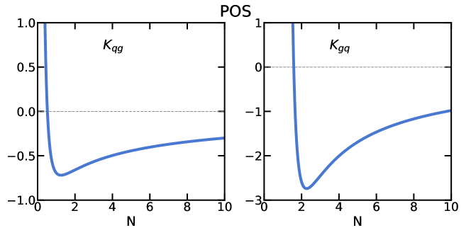
Figure 4: The off-diagonal elements of the NLO scheme change matrix $K^{\rm POS}$, Eq. (76), in Mellin space.

The scheme change from POS to $\overline{\rm{MS}}$ can be determined using Eqs. (34-36) (quark channel) and Eqs. (44-46) (gluon channel). We have

$$\left[\mathbb{I}+\frac{\alpha_{s}}{2\pi}{C^{(1)}}^{{\overline{\rm{MS}}}}\right] =\left[\mathbb{I}+\frac{\alpha_{s}}{2\pi}{C^{(1)}}^{\rm POS}\right]\otimes\left[\mathbb{I}+\frac{\alpha_{s}}{2\pi}{C^{(1)}}^{\rm POS}\otimes\right]^{-1}\left[\mathbb{I}+\frac{\alpha_{s}}{2\pi}\left({C^{(1)}}^{\rm POS}+K^{\rm POS}\right)\right]$$ (74)

$$=\left[\mathbb{I}+\frac{\alpha_{s}}{2\pi}{C^{(1)}}^{\rm POS}\right]\left[\mathbb{I}+\otimes\frac{\alpha_{s}}{2\pi}K^{\rm POS}\right],$$ (75)

where in Eq. (75) we have written the inverse of the POS scheme coefficient functions in perturbative form according to Eq. (71). The matrix $K^{\rm POS}$ has the off-diagonal structure

$$K^{\rm POS}=\left[\ln\left(\frac{(1-z)^{2}}{z}\right)-1\right]\left(\begin{array}[]{cc}0&P_{qg}(z)\\ P_{gq}(z)&0\end{array}\right).$$ (76)

The off-diagonal matrix elements of the matrix are displayed in Fig. 4 in Mellin space. Writing the basic factorization formula Eq. (65) in the POS and $\overline{\rm{MS}}$ schemes, equating the results, and using Eq. (75) we get

$$f^{\rm POS}(Q^{2})=\left[\mathbb{I}+\frac{\alpha_{s}}{2\pi}K^{\rm POS}\otimes\right]f^{{\overline{\rm{MS}}}}(Q^{2})\,,$$ (77)

which gives the scheme change between the $\overline{\rm{MS}}$ and POS PDFs.

Inspection of Eq. (77) immediately shows a possible issue with the POS scheme. Indeed, as well known, momentum conservation implies the pair of relations between the second Mellin moments of splitting functions $\gamma_{qq}(2)+\gamma_{gq}(2)=0$ and $2n_{f}\gamma_{qg}(2)+\gamma_{gg}(2)=0$. This relation is verified in the $\overline{\rm{MS}}$ scheme: in order for it to remain true in any scheme obtained from $\overline{\rm{MS}}$, the scheme change matrix must satisfy

$$K_{qq}+K_{gq}=2n_{f}K_{qg}+K_{gg}\Big{|}_{N=2}=0\,,$$ (78)

where by $K_{ij}\Big{|}_{N=2}$ we denote the second Mellin moment of the scheme change matrix elements. This relation is not satisfied by the matrix defined in Eqs. (34-36,44-46).

It might therefore be worth considering a variant of the POS scheme, in which momentum conservation is enforced by adding to the diagonal elements of the scheme change matrix a contribution which enforces momentum conservation. This can be done e.g. by adding a soft function, which vanishes both as $z\to 1$ and $z\to 0$. We choose

$$f^{\rm MOM}(z)=60z^{2}(1-z)^{2}\,,$$ (79)

which has the property that its second Mellin moment equals one: $f^{\rm MOM}(N=2)=1$. We then define a MPOS scheme as that which is obtained from $\overline{\rm{MS}}$ through a scheme change matrix $K^{\rm MPOS}$ whose matrix elements satisfy

$$K^{\rm MPOS}_{qq}(z) =-f^{\rm MOM}(z)K^{\rm POS}_{gq}\Big{|}_{N=2}\,,$$ (80)

$$K^{\rm MPOS}_{qg}(z) =K^{\rm POS}_{qg}(z)\,,$$ (81)

$$K^{\rm MPOS}_{gq}(z) =K^{\rm POS}_{gq}(z)\,,$$ (82)

$$K^{\rm MPOS}_{gg}(z) =-2n_{f}f^{\rm MOM}(z)K^{\rm POS}_{qg}\Big{|}_{N=2}\,.$$ (83)

The MPOS scheme then automatically satisfies momentum conservation. Coefficient functions in the MPOS scheme are shown in Figs. 1-3. It is clear that coefficient functions, and thus PDFs, remain positive in the MPOS scheme: indeed, the off-diagonal coefficient functions are unchanged, while the diagonal NLO contributions are modified by a small correction which is offset by the large positive LO contribution, and in fact in the hadronic case leaves the NLO correction positive for all $z$. Hence the MPOS and POS schemes have the same positivity properties. We will thus not discuss the MPOS scheme any further and restrict the discussion for simplicity to the POS scheme.

A further observation is that the POS scheme has been constructed in Sect. 2.2 based on the kinematics of hadronic processes, namely by performing the collinear subtraction in off-diagonal channels at the scale $\mu_{h}^{2}$, Eq. (33). As discussed in Sect. 2.2.1, if this scheme is used for the computation of electroproduction processes for which the relevant scale is $\mu_{D}^{2}$, Eq. (17), leads to coefficient functions, and consequently PDFs, that are with stronger reason positive. More in general, the POS scheme has been constructed using universal properties of the collinear emission that only depend on the LO splitting functions and the choice of scale, which is determined by the general kinematics of hadronic processes, but otherwise process-independent. However, the positivity argument presented in this Section shows that this choice, whereas theoretically appealing, is by no means necessary. In fact, any physical scheme choice of the form of Eq. (68) can be used to construct a positive factorization scheme, by just picking a scheme choice such that the coefficient functions of the processes used to define the PDFs remain positive, and perturbative for all $\xi$. In any such scheme positivity of the PDFs holds. In fact, the simplest choice would be to pick as a positive factorization scheme the physical scheme itself, in which PDFs are positive by construction, as they are identified with physically observable cross sections.

3.2.2 The $\overline{\rm{MS}}$ scheme

Having concluded that we can take the POS scheme as representative of a wide class of positive factorization schemes, we now discuss its relation to the $\overline{\rm{MS}}$ scheme, and what it tells us about positivity of $\overline{\rm{MS}}$ PDFs.

Inverting the scheme change from $\overline{\rm{MS}}$ to POS perturbatively (see Eq. (77)) we obtain

$$f^{{\overline{\rm{MS}}}}(Q^{2})=\left[\mathbb{I}-\frac{\alpha_{s}}{2\pi}K^{\rm POS}\otimes\right]f^{\rm POS}(Q^{2})\,.$$ (84)

It is then clear that if the POS PDFs are positive, then so are the $\overline{\rm{MS}}$ ones, because the matrix $K^{\rm POS}$ vanishes on the diagonal, and it has negative matrix elements off the diagonal, so $-K^{\rm POS}$ in Eq. (84) is positive. The perturbative inversion is justified due to the fact that the non-vanishing off-diagonal matrix elements of the $K$ matrix are actually power-suppressed (i.e. next-to-eikonal) in the $z\to 1$ limit.

This can be seen more formally by considering the exact Mellin-space inverse of the scheme change matrix, Eq. (77):

$$\left[\mathbb{I}+\frac{\alpha_{s}}{2\pi}K^{\rm POS}(N)\right]^{-1}=\frac{1}{1-\left(\frac{\alpha_{s}}{2\pi}\right)^{2}K_{qg}(N)K_{gq}(N)}\left[\mathbb{I}-\frac{\alpha_{s}}{2\pi}K^{\rm POS}(N)\right],$$ (85)

where $K^{\rm POS}_{ij}(N)$ denote (by slight abuse of notation) the Mellin transforms of the matrix elements $K^{\rm POS}_{ij}$ of the matrix $K^{\rm POS}$. It is easy to check that the factor $K_{qg}(N)K_{gq}(N)$ is a monotonically decreasing function of $N$ along the real $N$ axis, and in particular it vanishes as $\frac{1}{N^{2}}$ as $N\to\infty$, hence the prefactor which relates the exact and perturbative inversions, Eqs. (84-85), is actually bounded in the region $N\gtrsim 2$ in which the $\overline{\rm{MS}}$ coefficient functions, and thus the matrix elements of $K$, turn negative (see Figs. 2-3).

We conclude that the light quark and gluon $\overline{\rm{MS}}$ PDFs are in fact positive at NLO.

Heavy quarks require a separate discussion, because for heavy quarks $\overline{\rm{MS}}$ factorization can be defined in a variety of ways (see e.g. [21]). Specifically, heavy quarks can be treated in a massive scheme, in which collinear singularities associated to them are regulated by their mass, so they decouple from perturbative evolution. In this scheme no collinear subtraction is performed for massive quarks, so their PDF is given by the unsubtracted Eq. (2) and thus it remains a positive (and scale-independent) probability distribution to all perturbative orders. Note that nothing prevents this heavy quark PDF from having an “intrinsic” component, of non-perturbative origin: however, in this factorization scheme, the heavy quark PDFs will be scale-independent, and thus positive at all scales.

However, it is also possible to treat the heavy quark in a massless $\overline{\rm{MS}}$ scheme, in which the heavy quark is treated like other massless quarks, namely the collinear singularity regulated by its mass is subtracted according to Eqs. (14,24), but with $\mu^{2}$ now replaced by the heavy quark mass. Calculations performed in this scheme, with heavy quark mass effects neglected, are accurate for scales much larger than the quark mass. However, the massless scheme is in principle formally defined for all scales, including at the heavy quark mass. This is sometimes done by using the massless scheme for all flavors, but discontinuously changing the number of flavors at a matching scale chosen equal to (or of order of) the heavy quark mass (zero-mass variable-flavor number scheme, ZM-VFNS [22]). Below the matching scale the ZM-VFNS coincides with the massive scheme (with non-evolving heavy quark PDF), and at the matching scale the heavy quark PDF changes discontinuously: the matching condition is the scheme transformation from the massive to the massless $\overline{\rm{MS}}$ (computed up to NNLO in Ref. [23]). This scheme transformation accounts for the fact that in the massive scheme the heavy quark decouples from the running, so loop corrections with the massive quark circulating in loops are included in the Wilson coefficient, and not in the operator matrix element, while in the massless scheme they are included in the operator normalization along with all other light quarks, but neglecting the quark mass when computing them.

When $Q^{2}\sim m_{h}^{2}$ this neglect is not justified, and the corresponding scheme transformation may ruin positivity of the PDF. Specifically, it is often assumed that the massive-scheme PDF vanishes at some scale $Q^{2}\sim m_{h}^{2}$, and it indeed appears reasonable to expect that the low-scale heavy quark scheme PDF if not vanishing, is rather smaller than light quark PDFs (see Refs. [24, 25]). However, if one determines the massless-scheme heavy quark PDF by starting with a vanishing massive-scheme PDFs, and using perturbative matching conditions, a negative result can be found — and is indeed found using standard light quark and gluon PDFs [26]. This is now possible because the massless-scheme heavy quark PDF is not defined by a matrix element of the form of Eq. (2), but rather, as the transformation of such an operator matrix element to a scheme in which the quark mass is neglected, but in a region in which the quark mass is not negligible. Of course, if $Q^{2}\gg m_{h}^{2}$ the mass does become negligible, the previous arguments apply, and positivity of the heavy quark PDF is restored. Hence, positivity of the heavy quark PDF in the messless scheme only holds at high enough $Q^{2}$ that mass corrections are negligible.

All the discussion so far has been pursued at NLO. However, the main structure of the argument remains true to all perturbative orders. In particular, it is true to all orders that the diagonal splitting functions are negative at large $z$: in fact, at large $z$ to all perturbative orders they behave as $\frac{1}{(1-z)_{+}}$ [15]. At higher perturbative orders, coefficient functions will contain plus distributions with higher order powers of $\ln(1-z)$, leading to the familiar rise in the partonic cross section which is predicted to all orders by threshold resummation [12, 13]. Off-diagonal channels, where negative contributions as $z\to 1$ may and indeed are expected to arise, remain power suppressed in this limit. It follows that the off-diagonal structure Eq. (76) of the matrix relating a positive scheme to $\overline{\rm{MS}}$ will hold true to all orders. The positivity argument of Sect. 3.2.2 is a direct consequence of this structure, and it will thus also hold to all orders.

4 Conclusions

The goal of this paper was the construction of a universal factorization scheme in which PDFs are non-negative. In order to attack the problem, we started from the observation that $\overline{\rm{MS}}$ partonic cross sections for typical electro- and hadro-production processes are not positive. This then implies that positivity of the PDFs is not guaranteed, since folding a negative partonic cross section with a positive PDF could lead to a negative physical cross section. We have then traced negative partonic cross sections to the way collinear subtraction is performed in $\overline{\rm{MS}}$ and specifically we have shown that it is due to over-subtraction, related to the choice of subtraction scale, and also the treatment of the average over gluon polarizations in $d$ dimensions. This loss of positivity only manifests itself in off-diagonal quark-gluon and gluon-quark channels.

A universal subtraction prescription which preserves positivity of the partonic cross section can then be constructed using hadronic kinematics, and shown to preserve positivity also in electroproduction kinematics. This prescription does not automatically respect momentum conservation, which however can be enforced with a soft modification of the subtraction procedure that does not affect its positivity properties. By performing collinear factorization in the standard approach of Refs. [8, 9] it is then possible to show that positivity of the PDFs, defined as probability distributions, is preserved at all stages, so PDFs remain positive.

In fact, this positivity is a manifestation of the fact that PDFs can always be defined in terms of a physical process: what PDFs do is to allow one to express the perturbative QCD prediction for a process in terms of that for another process. The definition of the PDFs can then be process-independent (as in $\overline{\rm{MS}}$) or process-dependent (as in so-called physical schemes [18, 19]). Its positivity will then be preserved provided only that the renormalization conditions, which fix the value of operator matrix elements that define the PDFs, preserves their interpretation as moments of a probability distribution. Effectively, this corresponds to choosing positive Wilson coefficients.

By considering a scheme in which PDFs are manifestly positive, and the transformation from it to $\overline{\rm{MS}}$, we have finally shown that in the $\overline{\rm{MS}}$ scheme PDFs remain positive, despite the fact that off-diagonal partonic cross sections are negative. From a physical point of view, this is a consequence of the fact that the $\overline{\rm{MS}}$ subtraction is actually strongly positive in the diagonal channels (where by “strongly” we mean that partonic functions tend to $+\infty$ towards kinematic boundaries). This then overwhelms the negative contribution from off-diagonal channels, while away from kinematic boundaries off-diagonal channels are perturbatively subleading.

Positivity of the PDFs is neither necessary nor sufficient for physical cross sections to be positive, as they ought to: it is not necessary, because it is possible that a negative PDF still leads to a positive hadronic cross section once folded with a suitable coefficient function, and it is not sufficient because in a scheme, such as $\overline{\rm{MS}}$, in which some partonic cross sections are negative it could well be that, while the true PDF must necessarily lead to positive measurable cross sections, an incorrectly determined PDF could lead to a negative cross section despite being positive.

In other words, it is not necessarily true that the region in PDF space which is excluded by the requirement of positivity of the PDF is the same as that which is excluded by requiring positivity of the cross sections. However, from the point of view of PDFs determination, knowing that PDFs must be positive in a given factorization scheme does provide a useful constraint, in that it excludes a region which does not have to be explored, though this restriction is not necessarily the most stringent one. It is natural to ask whether the positivity requirement could be more restrictive in some factorization schemes than others, but it is unclear whether and how this question could be answered. The question of optimizing the scheme choice from the point of view of positivity constraints, for the sake of PDFs determination, remains open for future investigation.

References

- [1] G. Altarelli, S. Forte, and G. Ridolfi, “On positivity of parton distributions,” Nucl. Phys. B534 (1998) 277–296, arXiv:hep-ph/9806345 [hep-ph].
- [2] S. Forte, G. Altarelli, and G. Ridolfi, “Are parton distributions positive?,” Nucl. Phys. Proc. Suppl. 74 (1999) 138–141, arXiv:hep-ph/9808462 [hep-ph]. [,138(1998)].
- [3] NNPDF Collaboration, R. D. Ball, L. Del Debbio, S. Forte, A. Guffanti, J. I. Latorre, A. Piccione, J. Rojo, and M. Ubiali, “A Determination of parton distributions with faithful uncertainty estimation,” Nucl. Phys. B809 (2009) 1–63, arXiv:0808.1231 [hep-ph]. [Erratum: Nucl. Phys.B816,293(2009)].
- [4] F. Faura, S. Iranipour, E. R. Nocera, J. Rojo, and M. Ubiali, “The Strangest Proton?,” arXiv:2009.00014 [hep-ph].
- [5] R. D. Ball, L. Del Debbio, S. Forte, A. Guffanti, J. I. Latorre, J. Rojo, and M. Ubiali, “A first unbiased global NLO determination of parton distributions and their uncertainties,” Nucl. Phys. B838 (2010) 136–206, arXiv:1002.4407 [hep-ph].
- [6] NNPDF Collaboration, R. D. Ball et al., “Parton distributions for the LHC Run II,” JHEP 04 (2015) 040, arXiv:1410.8849 [hep-ph].
- [7] R. K. Ellis, W. J. Stirling, and B. R. Webber, “QCD and collider physics,” Camb. Monogr. Part. Phys. Nucl. Phys. Cosmol. 8 (1996) 1–435.
- [8] J. C. Collins and D. E. Soper, “Parton Distribution and Decay Functions,” Nucl. Phys. B194 (1982) 445–492.
- [9] G. Curci, W. Furmanski, and R. Petronzio, “Evolution of Parton Densities Beyond Leading Order: The Nonsinglet Case,” Nucl. Phys. B175 (1980) 27–92.
- [10] J. Collins, Foundations of perturbative QCD, vol. 32. Cambridge University Press, 11, 2013.
- [11] M. Bonvini, S. Forte, and G. Ridolfi, “The Threshold region for Higgs production in gluon fusion,” Phys. Rev. Lett. 109 (2012) 102002, arXiv:1204.5473 [hep-ph].
- [12] S. Catani and L. Trentadue, “Resummation of the QCD Perturbative Series for Hard Processes,” Nucl. Phys. B327 (1989) 323–352.
- [13] G. F. Sterman, “Summation of Large Corrections to Short Distance Hadronic Cross-Sections,” Nucl. Phys. B281 (1987) 310–364.
- [14] S. Forte and G. Ridolfi, “Renormalization group approach to soft gluon resummation,” Nucl. Phys. B650 (2003) 229–270, arXiv:hep-ph/0209154 [hep-ph].
- [15] S. Albino and R. D. Ball, “Soft resummation of quark anomalous dimensions and coefficient functions in MS-bar factorization,” Phys. Lett. B513 (2001) 93–102, arXiv:hep-ph/0011133 [hep-ph].
- [16] S. Jadach, W. Płaczek, S. Sapeta, A. Siodmok, and M. Skrzypek, “Parton distribution functions in Monte Carlo factorisation scheme,” Eur. Phys. J. C76 no. 12, (2016) 649, arXiv:1606.00355 [hep-ph].
- [17] F. Maltoni, “Basics of QCD for the LHC: as a case study,” CERN Yellow Rep. School Proc. 2 (2018) 41–67.
- [18] S. Catani, “Comment on quarks and gluons at small x and the SDIS factorization scheme,” Z. Phys. C 70 (1996) 263–272, arXiv:hep-ph/9506357.
- [19] M. Diemoz, F. Ferroni, E. Longo, and G. Martinelli, “Parton Densities from Deep Inelastic Scattering to Hadronic Processes at Super Collider Energies,” Z. Phys. C 39 (1988) 21.
- [20] S. Jadach, “private communications,” 2020.
- [21] S. Forte, E. Laenen, P. Nason, and J. Rojo, “Heavy quarks in deep-inelastic scattering,” Nucl. Phys. B 834 (2010) 116–162, arXiv:1001.2312 [hep-ph].
- [22] M. Aivazis, J. C. Collins, F. I. Olness, and W.-K. Tung, “Leptoproduction of heavy quarks. 2. A Unified QCD formulation of charged and neutral current processes from fixed target to collider energies,” Phys. Rev. D 50 (1994) 3102–3118, arXiv:hep-ph/9312319.
- [23] M. Buza, Y. Matiounine, J. Smith, and W. van Neerven, “Charm electroproduction viewed in the variable flavor number scheme versus fixed order perturbation theory,” Eur. Phys. J. C 1 (1998) 301–320, arXiv:hep-ph/9612398.
- [24] R. D. Ball, M. Bonvini, and L. Rottoli, “Charm in Deep-Inelastic Scattering,” JHEP 11 (2015) 122, arXiv:1510.02491 [hep-ph].
- [25] NNPDF Collaboration, R. D. Ball, V. Bertone, M. Bonvini, S. Carrazza, S. Forte, A. Guffanti, N. P. Hartland, J. Rojo, and L. Rottoli, “A Determination of the Charm Content of the Proton,” Eur. Phys. J. C 76 no. 11, (2016) 647, arXiv:1605.06515 [hep-ph].
- [26] NNPDF Collaboration, R. D. Ball et al., “Parton distributions from high-precision collider data,” Eur. Phys. J. C77 no. 10, (2017) 663, arXiv:1706.00428 [hep-ph].