Detecting relevant differences in the covariance operators of functional time series - a sup-norm approach

Abstract

In this paper we propose statistical inference tools for the covariance operators of functional time series in the two sample and change point problem. In contrast to most of the literature the focus of our approach is not testing the null hypothesis of exact equality of the covariance operators. Instead we propose to formulate the null hypotheses in the form that “the distance between the operators is small”, where we measure deviations by the sup-norm. We provide powerful bootstrap tests for these type of hypotheses, investigate their asymptotic properties and study their finite sample properties by means of a simulation study.

Keywords: covariance operator, functional time series, two sample problems, change point problems, CUSUM, relevant hypotheses, Banach spaces, bootstrap
AMS Subject Classification: 62G10, 62M10

1 Introduction

The field of functional data analysis has found considerable attention in the statistical literature as in many applications the observed data points exhibit certain degrees of dependence and smoothness and thus may naturally be regarded as discretized functions. Introductions to this topic can be found in the monographs of Bosq, (2000), Ramsay and Silverman, (2005), Ferraty and Vieu, (2010), Horváth and Kokoszka, (2012) and Hsing and Eubank, (2015), among others. Interest may, for example, be in comparing characteristic parameters of the random functions from two different samples (two sample problem) or in investigating whether a certain parameter of a functional time series remains stable over time (change point problem). In most cases the considered parameters (such as the mean) are functions themselves, which makes the analysis of this type of problems challenging. In the present paper we investigate the second-order properties of a stationary functional time series which are contained in its covariance operators and important for the understanding of the smoothness of the stochastic fluctuations of the data (Kraus and Panaretos,, 2012). Most of the literature on this topic considers Hilbert space-valued random variables. The popularity of this approach is due to the fact that such a framework allows the development of dimension reduction techniques such as (functional) principal components. On the other hand dimension reduction may yield to a loss of information as data is projected on finite dimensional spaces, and several authors argue that it might be more reasonable to work in the space of functions directly (see, for example, Aue et al.,, 2018, for a recent reference).

In this paper we will develop methodology to compare the covariance operators of two functional time series and to detect changes in the covariance operator of a functional time series in the space of continuous functions defined on a compact interval. Thus - in contrast to most of the literature on this topic, which considers Hilbert space-valued objects - the random variables under consideration are (dependent) elements of a Banach space, and it is possible to compare the covariance operators in the sup-norm. Another important difference to the literature consists in the fact that the main focus of our approach is not on classical hypotheses of the form

(1.1) $$H_{0}:C_{1}=C_{2}\qquad\mbox{versus}\qquad\ H_{1}:C_{1}\not=C_{2}$$

where $C_{1}$ and $C_{2}$ are either the covariance operators corresponding to the two samples or to the covariance operator before and after a change point. In contrast we consider relevant hypotheses of the form

(1.2) $$H_{0}^{\Delta}:d(C_{1},C_{2})\leq\Delta\qquad\mbox{versus}\qquad H_{1}^{\Delta}:d(C_{1},C_{2})>\Delta$$

where $\Delta\geq 0$ is a given threshold and $d$ a suitable metric on the space of covariance operators (in our case the $\sup$-norm). Note that hypotheses of the form (1.2) contain the classical hypotheses in (1.1) as a special case for the choice $\Delta=0$, but we argue that the case $\Delta>0$ is at least of equal interest. In fact, in many applications it is obvious that $C_{1}$ and $C_{2}$ can not exactly coincide but the deviation might be small. In such cases testing for exact equality may be questionable and it might be more reasonable to test for a relevant or significant deviation between the two covariance operators.

In the case of testing classical hypotheses the metric does not matter because under the null hypothesis the distance between $C_{1}$ and $C_{2}$ vanishes in any metric. However, this is not the case for relevant hypotheses of the form (1.2). In the present context two covariance operators with rather different shapes may still have a small $L^{2}$-distance, which makes an appropriate interpretation of the threshold $\Delta$ for practitioners difficult. As an alternative we propose to consider the maximum deviation between the covariance operators as metric in the hypotheses (1.2). On the one hand this metric makes the interpretation of the threshold $\Delta$ more easy. On the other hand it leads to a Banach space-based framework where no dimension reduction techniques are available and the development and theoretical justification of statistical methods are more challenging.

In Section 2 we review some basic properties of random variables in the space of continuous functions. In particular we define moments of order two through injective tensor products. We also state a central limit theorem for a stationary Banach-space valued process, which will be the basis for all theoretical arguments given in this paper. In Section 3 we develop statistical methods for the comparison of covariance operators in the two sample problem. In particular a test is proposed for the null hypothesis of no relevant difference between the covariance operators from two independent samples. As a special (and substantially simpler case) we also construct a new test for the classical hypotheses (1.1) with a simple structure and nice statistical properties. Section 4 is devoted to the change point problem, where methodology is developed to detect changes in the covariance operator of a functional time series. In all cases we make use of a multiplier bootstrap procedure to obtain critical values for the proposed tests. The theoretical justification of all methods is given in Section 6, while Section 5 contains a detailed simulation study to investigate the finite sample properties of the proposed tests. Although classical hypotheses are not the main focus of our work we also compare the new tests for the classical hypotheses with some of the currently available methodology and demonstrate that they provide powerful alternatives to the procedures, which have been proposed in the literature so far.

1.1 Related literature

There exists a considerable amount of literature considering the comparison of covariance operators in the two sample problem, where random functions in the Hilbert space of square-integrable functions and the classical null hypothesis of equal covariance operators are investigated. Panaretos et al., (2010) consider independent Gaussian data and describe an application to DNA minicircle data. Fremdt et al., (2013) extend the theoretical findings of these authors to a more general model such that non-Gaussian curves are also covered. In both references, functional principal components (FPCs) are used for dimension reduction. Kraus and Panaretos, (2012) introduce the notion of a dispersion operator and propose a robust test, which is based on a truncated version of the Hilbert-Schmidt norm of a score operator defined via the dispersion operator. Zhang and Shao, (2015) propose a pivotal test procedure based on FPCs and self-normalization and also provide inference tools for the eigensystem of the covariance operators.

Several authors argue that dimension reduction may yield to a loss of information and propose alternative procedures for the comparison of covariance operators in the two sample problem. Pigoli et al., (2014) discuss different distance measures between covariance operators and develop a permutation test and Paparoditis and Sapatinas, (2016) propose a bootstrap test for the (classical) null hypothesis of equality of $K$ covariance operators. Cabassi et al., (2017) suggest to combine all pairwise comparisons between samples of independent data into a global test for this problem, where the Hilbert-Schmidt norm between the square roots of the covariance operators is used as a measure of deviation. Boente et al., (2018) provide a theoretical framework which clarifies the ability of the test to detect local alternatives. Pilavakis et al., (2020) develop a fully functional test for the equality of auto-covariance operators of temporally dependent time series, which is based on a moving block bootstrap. For independent data the $K$-sample problem has also been considered by Guo et al., (2016) who propose to estimate the supremum value of the sum of the squared differences between the estimated individual covariance functions and the pooled sample covariance function.

So far, the change point problem for covariance operators has found less attention in the literature. Jarušková, (2013) uses FPCs to develop a test for the existence of a change point, while Stoehr et al., (2019) use the circular block bootstrap to construct a change point test. In particular these authors develop a test based on dimension reduction and two procedures which take the full functional structure into account. A fully functional test has also been proposed by Sharipov and Wendler, (2019), who use a non overlapping block bootstrap to obtain critical values. More recently, Aue et al., (2020) propose statistical tests for detecting a change in the spectrum and in the trace of the covariance operator, respectively.

All these references consider the problem of testing classical hypotheses of the form (1.1). Recently Dette et al., 2020b propose a comparison of covariance operators in the two sample problem and in the context of change point analysis by testing relevant hypotheses of the form (1.2), where an $L^{2}$-distance is used as metric. However, in the context of testing relevant hypotheses the norm matters as two covariance operators might be close in one norm but not in another. In particular, relevant deviations between covariance operators in the sup-norm have - to our best knowledge - not been considered so far and requires a different methodology as the space under consideration is a Banach but not a Hilbert space. There does not exist so much literature on functional data analysis considering Banach spaces and exemplarily we mention the recent work of Dette et al., 2020a who considered relevant hypotheses for the mean function and Liebl and Reimherr, (2019), who developed confidence bands for functional parameters.

2 $C(T)$-valued random variables

In this paper we consider random variables taking values in the Banach space of real-valued and continuous functions defined on a compact set $T$ and denote this space by $C(T)$, which is equipped with the sup-norm $\|X\|_{\infty}=\max_{t\in T}|X(t)|$ for any $X\in C(T)$. The underlying probability space $(\Omega,\mathcal{A},\mathbb{P})$ is assumed to be complete and measurability is always meant with respect to the Borel $\sigma$-field generated by the open sets relative to the respective sup-norm.

Following Chapter 11 in Janson and Kaijser, (2015), we use injective tensor products to define moments of $C(T)$-valued random variables and note that $C(T)^{\check{\otimes}k}=C(T^{k})$ isometrically with the natural identification (Theorem 11.6). The $k$th moment of a $C(T)$-valued random variable $X$ exists, whenever $\mathbb{E}\big{[}\|X\|^{k}_{\infty}]<\infty$ (Theorem 11.25) and is defined by the function in $C(T)^{\check{\otimes}k}=C(T^{k})$, which maps $(t_{1},\dots,t_{k})\in T^{k}$ to

$$\mathbb{E}X^{\check{\otimes}k}(t_{1},\dots,t_{k})=\mathbb{E}\big{[}X(t_{1})\cdots X(t_{k})\big{]}$$

(Theorem 11.10). Throughout this paper, we write $X^{\check{\otimes}2}=X\check{\otimes}X$ for any $X\in C(T)$ and mean the function in $C(T^{2})$ defined by $(s,t)\mapsto X(s)X(t)$. Consequently, the covariance operator of a $C(T)$-valued random variable is defined by

$$C(\cdot,\cdot)=\mbox{Cov}(X(\cdot),X(\cdot))=\mathbb{E}\big{[}(X-\mu)^{\check{\otimes}2}(\cdot,\cdot)\big{]}\in C(T^{2})$$

where $\mu=\mathbb{E}[X]\in C(T)$ is the expectation of $X$.

Let $\rho$ denote a metric on $T$ such that $(T,\rho)$ is totally bounded, then the metric $\rho_{\max}$ on $T^{2}$ is defined through $\rho_{\max}((s,t),(s^{\prime},t^{\prime}))=\max\{\rho(s,s^{\prime}),\rho(t,t^{\prime})\}$ and the expression $D(\omega,\rho_{\max})$ denotes the packing number with respect to the metric $\rho_{\max}$ on $T^{2}$ that is the maximal number of $\omega$-seperated points in $T^{2}$ (Van der Vaart and Wellner,, 1996). Note that in this case $(T^{2},\rho_{\max})$ is totally bounded as well.

In order to describe the dependence in the data we introduce the concept $\varphi$-mixing and denote by $\mathbb{P}(G|F)$ the conditional probability of $G$ given $F$. For two $\sigma$-fields $\mathcal{F}$ and $\mathcal{G}$ we define the coefficient

(2.1) $$\phi(\mathcal{F},\mathcal{G})=\sup\big{\{}|\mathbb{P}(G|F)-\mathbb{P}(G)|\colon F\in\mathcal{F},~{}G\in\mathcal{G},~{}\mathbb{P}(F)>0\big{\}}\,.$$

For a given strictly stationary sequence $(\eta_{j})_{j\in\mathbb{N}}$ of random variables in $C(T)$, denote by $\mathcal{F}^{k^{\prime}}_{k}$ the $\sigma$-field generated by $(\eta_{j}\colon k\leq j\leq k^{\prime})$. Then, the $k$th $\varphi$-mixing coefficient of $(\eta_{j})_{j\in\mathbb{N}}$ is defined by

$$\varphi(k)=\sup_{k^{\prime}\in\mathbb{N}}\phi(\mathcal{F}_{1}^{k^{\prime}},\mathcal{F}_{k^{\prime}+k}^{\infty})$$

and the stationary time series $(\eta_{j})_{j\in\mathbb{N}}$ is called $\varphi$-mixing whenever the sequence of mixing coefficients converges to zero as $k\to\infty$.

Given the preceding discussion, the analysis of the covariance operators of random variables in $C(T)$ can in some sense be regarded to the analysis of $C(T^{2})$-valued random variables. More precisely, Theorem 11.7 in Janson and Kaijser, (2015) implies that $C(T^{2})$ is separable such that measurability issues are avoided, and Theorem 1.3 in Billingsley, (1968) implies that any $C(T^{2})$-valued random variable is tight. A random function $X$ in $C(T^{2})$ is called Gaussian if and only if its finite dimensional vectors $(X(t_{1}),\dots,X(t_{k}))$ follow a multivariate normal distribution for any $t_{1},\dots,t_{k}\in T^{2}$ and $k\in\mathbb{N}$.

Assumption 2.1.

$(Z_{j})_{j\in\mathbb{N}}$ is a sequence of $C(T)$-valued random variables such that

$$Z_{j}=\mu+\eta_{j}\,,\quad j\in\mathbb{N}$$

where $\mu\in C(T)$ denotes the expectation function and $(\eta_{j})_{j\in\mathbb{N}}$ is a strictly stationary process.

1. The packing number $D(\omega,\rho_{\max})$ satisfies

   $$\int_{0}^{\tau}D(\omega,\rho_{\max})^{1/J}~{}d\omega<\infty$$

   for some $\tau>0$ and some even integer $J\geq 2$.

2. There is a constant $K$ such that

   $$\mathbb{E}[\|\eta_{1}\|_{\infty}^{4+\nu}]\leq K\,,\quad\mathbb{E}[\|\eta_{1}\|_{\infty}^{2J}]\leq\infty$$

   for some $\nu>0$, where $J$ is the same integer as in (A1).

3. There exists a real-valued non-negative random variable $M$ and a constant $\tilde{K}$ such that, for any $j\in\mathbb{N}$, $\mathbb{E}\big{[}(\|\eta_{j}\|_{\infty}\,M)^{J}\big{]}<\tilde{K}<\infty$ and the inequality

   $$|\eta_{j}(t)-\eta_{j}(t^{\prime})|\leq M\rho(t,t^{\prime})$$

   holds almost surely for all $t,t^{\prime}\in T$. The integer $J$ is the same as in (A1).

4. The process $(\eta_{j})_{j\in\mathbb{N}}$ is $\varphi$-mixing with mixing coefficients satisfying, for some $\bar{\tau}\in(1/(2+2\nu),1/2)$, the condition

   $$\sum_{k=1}^{\infty}k^{1/(1/2-\bar{\tau})}\varphi(k)^{1/2}<\infty\,,\quad\sum_{k=1}^{\infty}(k+1)^{J/2-1}\varphi(k)^{1/J}<\infty\,,$$

   where the constants $J$ and $\nu$ are the same as in (A1) and (A2), respectively.

Note that Assumption 2.1 implies the existence of the covariance operator defined by

(2.2) $$C(s,t)=\mbox{Cov}(Z_{j}(s),Z_{j}(t))=\mathbb{E}[(Z_{j}(s)-\mu(s))(Z_{j}(t)-\mu(t))]\,.$$

Condition (A4) on the summability of the mixing coefficients is satisfied if there exists an $a\in(0,1)$ such that $\varphi(k)\leq ca^{k}$ ($k\in\mathbb{N}$). For the formulation and a proof of a CLT of Banach space valued random variables we denote by the symbol “$\rightsquigarrow$” weak convergence in $(C(T))^{k}$ or $(C(T^{2}))^{k}$ and the symbol “$\stackrel{{\scriptstyle\mathcal{D}}}{{\longrightarrow}}$” denotes weak convergence in $\mathbb{R}^{k}$ for some $k\in\mathbb{N}$. The following result is proved in Section 6.

Theorem 2.1.

Let $(Z_{j})_{j\in\mathbb{N}}$ denote a stochastic process in $C(T)$ satisfying Assumption 2.1. Then,

$$G_{n}=\frac{1}{\sqrt{n}}\sum_{j=1}^{n}((Z_{j}-\bar{Z}_{n})^{\check{\otimes}2}-C)\rightsquigarrow Z$$

in $C(T^{2})$ as $n\to\infty$ where $\bar{Z}_{n}=1/n\sum_{j=1}^{n}Z_{j}\in C(T)$, $C$ is defined by (2.2) and $Z$ is a centred Gaussian random variable with covariance operator

(2.3) $$\mathbb{C}((s,t),(s^{\prime},t^{\prime}))=\mathrm{Cov}(Z(s,t),Z(s^{\prime},t^{\prime}))=\sum_{i=-\infty}^{\infty}\mbox{Cov}\big{(}\eta_{0}^{\check{\otimes}2}(s,t),\eta_{i}^{\check{\otimes}2}(s^{\prime},t^{\prime})\big{)}\,.$$

In the remaining part of the paper, we consider the unit interval $T=[0,1]$ and, for a positive constant $\theta\in(0,1]$, the metric $\rho(s,t)=|s-t|^{\theta}$ on $[0,1]$. Consequently, on $T^{2}=[0,1]^{2}$, we use the metric $\rho_{\max}((s,t),(s^{\prime},t^{\prime}))=\max\{\rho(s,s^{\prime}),\rho(t,t^{\prime})\}$ and the packing number of the square $[0,1]^{2}$ with respect to this metric satisfies $D(\omega,\rho_{\max})\lesssim\big{\lceil}\omega^{-2/\theta}\big{\rceil}$ (to see this, consider the points $(k\omega^{1/\theta},l\omega^{1/\theta})$ for $k,l=0,\dots,\lfloor\omega^{-1/\theta}\rfloor$). Therefore condition (A1) reduces to

$$\int_{0}^{\tau}D(\omega,\rho_{\max})^{1/J}~{}d\omega \lesssim\int_{0}^{\tau}\big{\lceil}\omega^{-2/\theta}\big{\rceil}^{1/J}~{}d\omega\lesssim\frac{\tau^{1-2/(J\theta)}}{1-2/(J\theta)}<\infty$$

and holds, whenever the even integer $J$ satisfies $J>2/\theta$ and consequently, under this assumption, Hölder continuous processes satisfy (A1). Because the paths of the Brownian Motion $\{W(t)\}_{t\in[0,1]}$ are Hölder continuous of order $\theta$ for any $\theta\in(0,1/2)$ and the random variable $\|W\|_{\infty}$ has moments of all order Assumption 2.1 is satisfied for the Brownian motion (we can use $J=6$ in (A4) for this case). For general processes with less smoothness, that is a smaller constant $\theta$, we require a stronger summability assumption (A4) on the mixing coefficients and the existence of higher moments.

3 The two sample problem

Throughout this section, we consider two independent samples $(X_{j}\colon j=1,\dots,m)$ and $(Y_{j}\colon j=1,\dots,n)$ drawn from independent strictly stationary sequences $(X_{j})_{j\in\mathbb{N}}$ and $(Y_{j})_{j\in\mathbb{N}}$ in $C([0,1])$ with representations

(3.1) $$X_{j}=\mu_{1}+\eta_{1,j}\,,\quad Y_{j}=\mu_{2}+\eta_{2,j}\,,$$

where $\mu_{1},\mu_{2}\in C([0,1])$ and $(\eta_{1,j})_{j\in\mathbb{N}}$, $(\eta_{2,j})_{j\in\mathbb{N}}$ are centred $C([0,1])$-valued processes satisfying the following assumption.

Assumption 3.1.

The processes $(\eta_{1,j})_{j\in\mathbb{N}}$, $(\eta_{2,j})_{j\in\mathbb{N}}$ are independent centred strictly stationary processes satisfying Assumption 2.1 with metric $\rho(s,t)=|t-s|^{\theta}$ for some $\theta>0$ such that $J\theta>2$.

In the following let

$$C_{1}(s,t) =\mathbb{E}[\eta_{1,j}(s)\eta_{1,j}(t)]=\mbox{Cov}(X_{1}(s),X_{1}(t))\,,$$

$$C_{2}(s,t) =\mathbb{E}[\eta_{2,j}(s)\eta_{2,j}(t)]=\mbox{Cov}(Y_{1}(s),Y_{1}(t))$$

denote the covariance operator of the first and the second sample, respectively. We measure the difference between $C_{1}$ and $C_{2}$ by their maximal deviation

(3.2) $$d_{\infty}=\|C_{1}-C_{2}||_{\infty}=\sup_{s,t\in[0,1]}|C_{1}(s,t)-C_{2}(s,t)|\,,$$

and are interested in testing if there exists a relevant difference between the covariance operators, that is

(3.3) $$H^{\Delta}_{0}:d_{\infty}\ \leq\Delta\qquad\mbox{versus}\qquad H^{\Delta}_{1}:d_{\infty}>\Delta\,,$$

where $\Delta\in\mathbb{R}$ is a pre-specified constant. Note that the classical hypotheses

(3.4) $$H_{0}:C_{1}=C_{2}\qquad\mbox{versus}\qquad H_{1}:C_{1}\neq C_{2}$$

are obtained for the choice $\Delta=0$.

We denote by $\tilde{X}_{m,j}=X_{j}-\bar{X}_{m},\,\tilde{Y}_{n,i}=Y_{i}-\bar{Y}_{n}$ the centred random curves (here $\bar{X}_{m}$ and $\bar{Y}_{n}$ denote the mean in the first and second sample, respecively), and estimate the maximal deviation $d_{\infty}$ in (3.2) between the two covariance operators by

(3.5) $$\hat{d}_{\infty}:=\sup_{s,t\in[0,1]}\bigg{|}\frac{1}{m-1}\sum_{j=1}^{m}\tilde{X}_{m,j}^{\check{\otimes}2}(s,t)-\,\frac{1}{n-1}\sum_{j=1}^{n}\tilde{Y}_{n,j}^{\check{\otimes}2}(s,t)\bigg{|}\,.$$

Now a reasonable decision rule is to reject the null hypothesis in (3.3) or (3.4) for large values of $\hat{d}_{\infty}$. Our first result provides the asymptotic properties of the statistic $\hat{d}_{\infty}$.

Proposition 3.1.

If $\mu_{1},\mu_{2}\in C([0,1])$ and $(\eta_{1,j})_{j\in\mathbb{N}}$, $(\eta_{2,j})_{j\in\mathbb{N}}$ are strictly stationary and centred $C([0,1])$-valued processes satisfying Assumption 3.1 and $\frac{m}{m+n}\longrightarrow\lambda\in(0,1)$ as $m,n\to\infty$, the following assertions hold true.

• If $d_{\infty}=0$, then

  (3.6) $$\sqrt{m+n}\,\hat{d}_{\infty}\stackrel{{\scriptstyle\mathcal{D}}}{{\longrightarrow}}T=\sup_{s,t\in[0,1]}|Z(s,t)|\,,$$

  where $Z$ is a Gaussian random element in $C([0,1]^{2})$ with covariance operator

  (3.7) $$\mathbb{C}=\frac{1}{\lambda}~{}\mathbb{C}_{1}-\frac{1}{1-\lambda}~{}\mathbb{C}_{2}\,,$$

  and $\mathbb{C}_{1}$ and $\mathbb{C}_{2}$ are the long-run covariance operators defined by

  (3.8) $$\mathbb{C}_{1}((s,t),(s^{\prime},t^{\prime})) =\sum_{i=-\infty}^{\infty}\mbox{Cov}\big{(}\eta_{1,0}^{\check{\otimes}2}(s,t),\eta_{1,i}^{\check{\otimes}2}(s^{\prime},t^{\prime})\big{)}\,,$$

  (3.9) $$\mathbb{C}_{2}((s,t),(s^{\prime},t^{\prime})) =\sum_{i=-\infty}^{\infty}\mbox{Cov}\big{(}\eta_{2,0}^{\check{\otimes}2}(s,t),\eta_{2,i}^{\check{\otimes}2}(s^{\prime},t^{\prime})\big{)}\,.$$

• If $d_{\infty}>0$, we have

  (3.10) $$\sqrt{m+n}\,(\hat{d}_{\infty}-d_{\infty})\stackrel{{\scriptstyle\mathcal{D}}}{{\longrightarrow}}T({\cal E})=\max\Big{\{}\sup_{(s,t)\in{\cal E}^{+}}Z(s,t),\sup_{(s,t)\in{\cal E}^{-}}-Z(s,t)\Big{\}}\,,$$

  where $Z$ is a Gaussian random element in $C([0,1]^{2})$ with covariance operator defined by (3.7) and

  (3.11) $$\mathcal{E}^{\pm}=\big{\{}(s,t)\in[0,1]^{2}\colon C_{1}(s,t)-C_{2}(s,t)={\pm}d_{\infty}\big{\}}$$

  are the extremal sets of the difference of the covariance operators $C_{1},C_{2}$.

If $u_{1-\alpha}$ denotes the $(1-\alpha)$-quantile of the distribution of the random variable $T$ defined in (3.6), a consistent and asymptotic level $\alpha$ tests for the classical hypotheses in (3.4) can be obtained by rejecting the null hypothesis, whenever

$$\hat{d}_{\infty}>\frac{u_{1-\alpha}}{\sqrt{m+n}}\,.$$

Similarly, the null hypothesis in (3.3) is rejected if

$$\hat{d}_{\infty}>\Delta+\frac{u_{1-\alpha,{\cal E}}}{\sqrt{m+n}}$$

where $u_{1-\alpha,{\cal E}}$ is the $\alpha$-quantile of the distribution of the random variable $T(\cal E)$ defined in (3.10). However, the quantile $u_{1-\alpha}$ depends on the long-run covariance operators $\mathbb{C}_{1}$ and $\mathbb{C}_{2}$ which are difficult to estimate. For the problem of testing relevant hypotheses the situation is even more complicated as the quantile $u_{1-\alpha,{\cal E}}$ additionally depends on the unknown extremal sets defined in (3.11), which have to be estimated as well. To deal with these problems we propose a bootstrap approach, which is explained for the classical and relevant hypotheses separately.

3.1 Classical hypotheses

In order to avoid the problem of estimating the long-run covariance operators we propose a bootstrap procedure to mimic the covariance structure of the distribution of the process

$$\frac{1}{m-1}\sum_{j=1}^{m}\tilde{X}_{m,j}^{\check{\otimes}2}-\,\frac{1}{n-1}\sum_{j=1}^{n}\tilde{Y}_{n,j}^{\check{\otimes}2}-(C_{1}-C_{2})$$

by a multiplier bootstrap process (note that the second term vanishes in the case $d_{\infty}=0$). To be precise, we denote by $(\xi_{k}^{(1)})_{k\in\mathbb{N}},\ldots,$ $(\xi_{k}^{(R)})_{k\in\mathbb{N}}$ and $(\zeta_{k}^{(1)})_{k\in\mathbb{N}},\ldots,$ $(\zeta_{k}^{(R)})_{k\in\mathbb{N}}$ independent sequences of independent standard normal distributed random variables and define the $C([0,1]^{2})$-valued processes $\hat{B}_{m,n}^{(1)},$ $\ldots,$ $\hat{B}_{m,n}^{(R)}$ by

(3.12) $$\begin{split}\hat{B}_{m,n}^{(r)}=\sqrt{n+m}\bigg{\{}&\frac{1}{m}\sum_{k=1}^{m-l_{1}+1}\frac{1}{\sqrt{l_{1}}}\bigg{(}\sum_{j=k}^{k+l_{1}-1}\tilde{X}_{m,j}^{\check{\otimes}2}-\frac{l_{1}}{m}\sum_{i=1}^{m}\tilde{X}_{m,i}^{\check{\otimes}2}\bigg{)}\xi_{k}^{(r)}\\ -&\frac{1}{n}\sum_{k=1}^{n-l_{2}+1}\frac{1}{\sqrt{l_{2}}}\bigg{(}\sum_{j=k}^{k+l_{2}-1}\tilde{Y}_{n,j}^{\check{\otimes}2}-\frac{l_{2}}{n}\sum_{i=1}^{n}\tilde{Y}_{n,i}^{\check{\otimes}2}\bigg{)}\zeta_{k}^{(r)}\bigg{\}}~{}~{}~{}~{}(r=1,\ldots,R)\,.\end{split}$$

The parameters $l_{1},l_{2}\in\mathbb{N}$ define the block length such that $l_{1}/m\to 0$ and $l_{2}/n\to 0$ as $l_{1},l_{2},m,n\to\infty$. Note that the dependence on $l_{1}$ and $l_{2}$ is not reflected in the notation of the bootstrap processes. With these notations we define the bootstrap statistics

(3.13) $$T_{m,n}^{(r)}=\sup_{s,t\in[0,1]}|\hat{B}_{m,n}^{(r)}(s,t)|~{}~{}~{}~{}(r=1,\dots,R)\,,$$

and denote by $T_{m,n}^{\{\lfloor R(1-\alpha)\rfloor\}}$ the empirical $(1-\alpha)$-quantile of the bootstrap sample $T_{m,n}^{(1)},\dots,T_{m,n}^{(R)}$. Then, rejecting the classical null hypothesis of equal covariance operators whenever

(3.14) $$\hat{d}_{\infty}>\frac{T_{m,n}^{\{\lfloor R(1-\alpha)\rfloor\}}}{\sqrt{m+n}}$$

defines a bootstrap test for the classical hypotheses in (3.4). The following result provides the statistical properties of this test.

Theorem 3.1.

Suppose that the error processes $(\eta_{1,j})_{j\in\mathbb{N}}$ and $(\eta_{2,j})_{j\in\mathbb{N}}$ in the representation (3.1) satisfy Assumption 3.1. Let $\hat{B}_{m,n}^{(1)},\ldots,\hat{B}_{m,n}^{(R)}$ denote the bootstrap processes defined by (3.12) such that $l_{1}=m^{\beta_{1}}$, $l_{2}=n^{\beta_{2}}$ with

$$0<\beta_{i}<\nu_{i}/(2+\nu_{i})~{},~{}~{}\bar{\tau}_{i}>(\beta_{i}(2+\nu_{i})+1)/(2+2\nu_{i})$$

where $\bar{\tau}_{i},\nu_{i}$ are given in Assumption 2.1, $i=1,2$.

Then, under the classical null hypothesis $H_{0}:C_{1}=C_{2}$ in (3.4) we have

(3.15) $$\lim_{m,n,R\to\infty}\mathbb{P}\bigg{(}\hat{d}_{\infty}>\frac{T_{m,n}^{\{\lfloor R(1-\alpha)\rfloor\}}}{\sqrt{m+n}}\bigg{)}=\alpha\,.$$

Under the alternative $H_{1}:C_{1}\not=C_{2}$ in (3.4) it follows for any $R\in\mathbb{N}$,

(3.16) $$\liminf_{m,n\to\infty}\mathbb{P}\bigg{(}\hat{d}_{\infty}>\frac{T_{m,n}^{\{\lfloor R(1-\alpha)\rfloor\}}}{\sqrt{m+n}}\bigg{)}=1\,.$$

3.2 Relevant hypotheses

For testing relevant hypotheses it is crucial to estimate the extremal sets in (3.11) properly. For this purpose we propose

(3.17) $$\hat{\mathcal{E}}_{m,n}^{\pm} =\Big{\{}(s,t)\in[0,1]^{2}\colon\pm\big{(}\hat{C}_{1}(s,t)-\hat{C}_{2}(s,t)\big{)}\geq\hat{d}_{\infty}-\frac{c_{m,n}}{\sqrt{m+n}}\ \Big{\}}$$

as estimators of the sets $\cal E^{\pm}$ where $(c_{m,n})_{m,n\in\mathbb{N}}$ is a sequence of positive constants satisfying $\lim_{m,n\to\infty}c_{m,n}/\log(m+n)=c$ for some $c>0$. For the construction of a test of the relevant hypotheses in (3.3) we recall the definition of the bootstrap process in (3.12) and define the statistics

(3.18) $$K^{(r)}_{m,n}=\max\Big{\{}\sup_{(s,t)\in\hat{\mathcal{E}}_{m,n}^{+}}\hat{B}_{m,n}^{(r)}(s,t),\ \sup_{(s,t)\in\hat{\mathcal{E}}_{m,n}^{-}}\big{(}-\hat{B}_{m,n}^{(r)}(s,t)\big{)}\Big{\}}\quad\quad(r=1,\dots,R)\,$$

which serves as the bootstrap analogue of the statistic $T({\cal E})$ defined in (3.10). If $K_{m,n}^{\{\lfloor R(1-\alpha)\rfloor\}}$ denotes the empirical $(1-\alpha)$-quantile of the bootstrap sample $K_{m,n}^{(1)},\dots,K_{m,n}^{(R)}$ we propose to reject the null hypothesis of no relevant difference in the covariance operators at level $\alpha$, whenever

(3.19) $$\hat{d}_{\infty}>\Delta+\frac{K_{m,n}^{\{\lfloor R(1-\alpha)\rfloor\}}}{\sqrt{m+n}}\,.$$

The final result of this section states that this test is consistent and has asymptotic level $\alpha$.

Theorem 3.2.

Suppose that the assumptions of Theorem 3.1 are satisfied and that $\Delta>0$.

• Under the null hypothesis $H_{0}:d_{\infty}\leq\Delta$ of no relevant difference in the covariance operators, it follows

  (3.20) $$\lim_{m,n,R\to\infty}\mathbb{P}\bigg{(}\hat{d}_{\infty}>\Delta+\frac{K_{m,n}^{\{\lfloor R(1-\alpha)\rfloor\}}}{\sqrt{m+n}}\bigg{)}=\alpha\,,$$

  if $\Delta=d_{\infty}$ and, for any $R\in\mathbb{N}$,

  $$\lim_{m,n\to\infty}\mathbb{P}\bigg{(}\hat{d}_{\infty}>\Delta+\frac{K_{m,n}^{\{\lfloor R(1-\alpha)\rfloor\}}}{\sqrt{m+n}}\bigg{)}=0\,,$$

  if $0<d_{\infty}<\Delta$.

• Under the alternative $H_{1}:d_{\infty}>\Delta$ of a relevant difference in the covariance operators it follows for any $R\in\mathbb{N}$

  $$\liminf_{m,n\to\infty}\mathbb{P}\bigg{(}\hat{d}_{\infty}>\Delta+\frac{K_{m,n}^{\{\lfloor R(1-\alpha)\rfloor\}}}{\sqrt{m+n}}\bigg{)}=1\,.$$

4 Detecting changes in the covariance operator

In this section we study the change point problem for the covariance operator of an array $(X_{n,j}\colon n\in\mathbb{N},j=1,\dots,n)$ of $C([0,1])$-valued random variables. For the consideration of relevant changes we require a dependence concept for an array $(\tilde{\eta}_{n,j}\colon n\in\mathbb{N},j=1,\dots,n)$ of random variables in $C(T)$ with strictly stationary rows. For this purpose we denote by $\mathcal{F}^{k^{\prime}}_{k,n}$ the $\sigma$-field generated by $(\tilde{\eta}_{n,j}\colon k\leq j\leq k^{\prime})$. The $k$th $\varphi$-mixing coefficient of the array $(\tilde{\eta}_{n,j}\colon n\in\mathbb{N},j=1,\dots,n)$ is then defined by

$$\varphi(k)=\sup_{n\in\mathbb{N}}\sup_{k^{\prime}\in\{1,\dots,n-k\}}\phi(\mathcal{F}_{1,n}^{k^{\prime}},\mathcal{F}_{k^{\prime}+k,n}^{n})$$

and $(\tilde{\eta}_{n,j}\colon n\in\mathbb{N},j=1,\dots,n)$ is called $\varphi$-mixing whenever $\varphi(k)\to 0$ as $k\to\infty$. For our theoretical investigations we make the following assumption.

Assumption 4.1.

For some $\vartheta\in(0,\frac{1}{2}]$ there exists a number $s^{*}\in[\vartheta,1-\vartheta]$ such that the random variables $(X_{n,j}\colon n\in\mathbb{N},j=1,\dots,n)$ are given by $X_{n,j}=\mu+\tilde{\eta}_{n,j}$, where $\mu=\mathbb{E}[X_{n,j}]$ denotes the common expectation function,

(4.1) $$\tilde{\eta}_{n,j}=\begin{cases}\eta_{1,j}\quad\text{ if }~{}j\in\{1,\dots,\lfloor s^{*}n\rfloor\}\\ \eta_{2,j}\quad\text{ if }~{}j\in\{\lfloor s^{*}n\rfloor+1,\dots,n\}\end{cases}$$

and $(\eta_{1,j})_{n\in\mathbb{N}}$, $(\eta_{2,j})_{n\in\mathbb{N}}$ are centred strictly stationary processes satisfying conditions (A1) - (A3) of Assumption 2.1 with metric $\rho(s,t)=|s-t|^{\theta}$ for some $\theta>0$ such that $\theta J>2$. Furthermore it is assumed that the array $(\tilde{\eta}_{n,j}\colon n\in\mathbb{N},j=1,\dots,n)$ is $\varphi$-mixing with mixing coefficients satisfying condition (A4) of Assumption 2.1.

We denote by $C_{1}$ and $C_{2}$ the covariance operator before and after the change point. Recalling the definition of $d_{\infty}$ in (3.2) the relevant and classical hypotheses are given by (3.3) and (3.4), respectively. For the construction of a test for these hypotheses we consider a sequential empirical process on $C([0,1]^{3})$ defined by

(4.2) $$\hat{\mathbb{U}}_{n}(s,t,u)=\frac{1}{n}\Big{(}\sum^{\lfloor sn\rfloor}_{j=1}\tilde{X}_{n,j}^{\check{\otimes}2}(t,u)+n\Big{(}s-\frac{\lfloor sn\rfloor}{n}\Big{)}\tilde{X}_{n,\lfloor sn\rfloor+1}^{\check{\otimes}2}(t,u)-s\sum^{n}_{j=1}\tilde{X}_{n,j}^{\check{\otimes}2}(t,u)\Big{)}$$

where $\tilde{X}_{n,j}=X_{n,j}-\bar{X}_{n}$ $(j=1,\dots,n;~{}n\in\mathbb{N})$ and note that it can be shown that

$$\mathbb{E}\big{[}\hat{\mathbb{U}}_{n}(s,t,u)\big{]}=\big{(}s\wedge s^{*}-ss^{*}\big{)}\big{(}C_{1}(t,u)-C_{2}(t,u)\big{)}+o_{\mathbb{P}}(1)\,.$$

Consequently, it is reasonable to consider the statistic

(4.3) $$\mathbb{\hat{M}}_{n}=\sup_{s\in[0,1]}\sup_{t,u\in[0,1]}|\hat{\mathbb{U}}_{n}(s,t,u)|$$

as an estimate of

$$s^{*}(1-s^{*})\,d_{\infty}=s^{*}(1-s^{*})\,\|C_{1}-C_{2}\|_{\infty}\,.$$

The following result makes these heuristic arguments precise.

Proposition 4.1.

If Assumption 4.1 is satisfied, the following statements hold true.

• If $d_{\infty}=0$, then

  (4.4) $$\sqrt{n}\,\mathbb{\hat{M}}_{n}\stackrel{{\scriptstyle\cal D}}{{\longrightarrow}}\check{T}=\sup_{(s,t,u)\in[0,1]^{3}}|\mathbb{W}(s,t,u)|$$

  where $\mathbb{W}$ is a Gaussian random element in $C([0,1]^{3})$ with covariance operator

  (4.5) $$\begin{split}\mbox{Cov}&(\mathbb{W}(s,t,u),\mathbb{W}(s^{\prime},t^{\prime},u^{\prime}))\\ =&\big{\{}(s\wedge s^{\prime}\wedge s^{*})+ss^{\prime}s^{*}-s(s^{\prime}\wedge s^{*})-s^{\prime}(s\wedge s^{*})\big{\}}\,\mathbb{C}_{1}((t,u),(t^{\prime},u^{\prime}))\,\\ &+\big{\{}(s\wedge s^{\prime}-s^{*})_{+}+ss^{\prime}(1-s^{*})-s(s^{\prime}-s^{*})_{+}-s^{\prime}(s-s^{*})_{+}\big{\}}\,\mathbb{C}_{2}((t,u),(t^{\prime},u^{\prime}))\end{split}$$

  and the long-run covariance operators $\mathbb{C}_{1},\mathbb{C}_{2}$ are defined by

  (4.6) $$\mathbb{C}_{l}((s,t),(s^{\prime},t^{\prime})) =\sum_{i=-\infty}^{\infty}\mbox{Cov}\big{(}\eta_{l,0}^{\check{\otimes}2}(s,t),\eta_{l,i}^{\check{\otimes}2}(s^{\prime},t^{\prime})\big{)}\quad\quad(l=1,2)\,.$$

• If $d_{\infty}>0$, we have

  (4.7) $$\begin{split}\sqrt{n}\big{(}\mathbb{\hat{M}}_{n}-s^{*}(1-s^{*})d_{\infty}\big{)}\stackrel{{\scriptstyle\cal D}}{{\longrightarrow}}\tilde{D}(\mathcal{E})=\max\Big{\{}\sup_{(t,u)\in\mathcal{E}^{+}}\mathbb{W}(s^{*},t,u),\sup_{(t,u)\in\mathcal{E}^{-}}-\mathbb{W}(s^{*},t,u)\Big{\}}\,,\end{split}$$

  where $\mathbb{W}$ is a Gaussian random element in $C([0,1]^{3})$ with covariance operator defined by (4.5) and $\mathcal{E}^{\pm}$ are the extremal sets defined in (3.11).

As in the two sample problem we can form decision rules, rejecting the null hypothesis (classical or relevant) for large values of $\mathbb{\hat{M}}_{n}$. Note that this requires estimation of the long-run covariance operators and (in the case of relevant hypotheses) the estimation of the change point and the extremal sets. For the construction of an explicit test (based on a multiplier bootstrap) we investigate again classical and relevant hypotheses separately.

4.1 Classical hypotheses

Most of the literature on change point analysis of covariance operators investigates the classical hypotheses of the form (3.4), where $C_{1}$ and $C_{2}$ denote the covariance operator before and after the change point (see Jarušková,, 2013; Sharipov and Wendler,, 2019; Stoehr et al.,, 2019). In order to obtain critical values for a test for a structural break in the covariance operators we consider a $C([0,1]^{3})$-valued bootstrap process defined by

(4.8) $$\begin{split}\hat{B}_{n}^{(r)}(s,t,u)=&\frac{1}{\sqrt{n}}\sum_{k=1}^{\lfloor sn\rfloor}\frac{1}{\sqrt{l}}\Big{(}\sum_{j=k}^{k+l-1}\hat{Y}_{n,j}(t,u)-\frac{l}{n}\sum_{j=1}^{n}\hat{Y}_{n,j}(t,u)\Big{)}\xi_{k}^{(r)}\\ &+\sqrt{n}\Big{(}s-\frac{\lfloor sn\rfloor}{n}\Big{)}\frac{1}{\sqrt{l}}\Big{(}\sum_{j=\lfloor sn\rfloor+1}^{\lfloor sn\rfloor+l}\hat{Y}_{n,j}(t,u)-\frac{l}{n}\sum_{j=1}^{n}\hat{Y}_{n,j}(t,u)\Big{)}\xi_{\lfloor sn\rfloor+1}^{(r)}\,,\end{split}$$

if $\lfloor sn\rfloor\leq n-l$, where $(\xi_{k}^{(1)})_{k\in\mathbb{N}},\ldots,(\xi_{k}^{(R)})_{k\in\mathbb{N}}$ denote independent sequences of independent Gaussian random variables with mean $0$ and variance $1$ and

$$\hat{Y}_{n,j}=\tilde{X}_{n,j}^{\check{\otimes}2}(t,u)-(\hat{C}_{2}-\hat{C}_{1})\mathds{1}\{j>\lfloor\hat{s}n\rfloor\}\quad\quad(j=1,\dots,n)\,.$$

The expressions

$$\hat{C}_{1}=\frac{1}{\lfloor\hat{s}n\rfloor}\sum_{j=1}^{\lfloor\hat{s}n\rfloor}\tilde{X}_{n,j}^{\check{\otimes}2}(t,u)\qquad\text{and}\qquad\hat{C}_{2}=\frac{1}{\lfloor(1-\hat{s})n\rfloor}\sum_{j=\lfloor\hat{s}n\rfloor+1}^{n}\tilde{X}_{n,j}^{\check{\otimes}2}(t,u)$$

are estimators of the covariance operator before and after the change point and

(4.9) $$\hat{s}=\max\Big{\{}\vartheta,\,\min\Big{\{}\frac{1}{n}\arg\max_{1\leq k<n}\big{\|}\hat{\mathbb{U}}_{n}(k/n,\cdot,\cdot)\big{\|}_{\infty},\,1-\vartheta\Big{\}}\Big{\}}$$

is an estimator of the unknown change location $s^{*}$ (note that $s^{*}\in(\vartheta,1-\vartheta)$ by assumption). In (4.8) the parameter $l\in\mathbb{N}$ denotes the block length satisfying $l/n\to 0$ as $l,n\to\infty$ and for any $t,u\in[0,1]$ and any $s\in[0,1]$ such that $\lfloor sn\rfloor>n-l$ we define

$$\hat{B}_{n}^{(r)}((n-l)/n,t,u)=\hat{B}_{n}^{(r)}(s,t,u)\,.$$

Finally, a bootstrap process is defined by

(4.10) $$\hat{\mathbb{W}}_{n}^{(r)}(s,t,u)=\hat{B}_{n}^{(r)}(s,t,u)-s\hat{B}_{n}^{(r)}(1,t,u)\quad\quad(r=1,\dots,R)$$

and we consider the bootstrap statistic

(4.11) $$\check{T}_{n}^{(r)}=\sup_{s,t,u\in[0,1]}\big{|}\hat{\mathbb{W}}_{n}^{(r)}(s,t,u)\big{|}\quad\quad(r=1,\dots,R)\,.$$

If $\check{T}_{n}^{\{\lfloor R(1-\alpha)\rfloor\}}$ denotes the empirical $(1-\alpha)$-quantile of the bootstrap sample $\check{T}_{n}^{(1)},\check{T}_{n}^{(2)},\dots,\check{T}_{n}^{(R)}$, the classical null hypothesis (3.4) of no change in the covariance operators is rejected, whenever

(4.12) $$\hat{\mathbb{M}}_{n}>\frac{\check{T}_{n}^{\{\lfloor R(1-\alpha)\rfloor\}}}{\sqrt{n}}\,.$$

Theorem 4.1.

Assume that the array $(X_{n,j}\colon n\in\mathbb{N},j=1,\dots,n)$ satisfies Assumption 4.1. Further assume that $l=n^{\beta}$ for some constant $\beta\in(1/5,2/7)$ such that the constant $\nu$ in (A2) satisfies $\nu\geq 4$ and

$$(\beta(2+\nu)+1)/(2+2\nu)<\bar{\tau}<1/2$$

where $\bar{\tau}$ is defined in (A4).

Then, under the classical null hypothesis $H_{0}:C_{1}=C_{2}$, we have

$$\lim_{n,R\to\infty}\mathbb{P}\bigg{(}\hat{\mathbb{M}}_{n}>\frac{\check{T}_{n}^{\{\lfloor R(1-\alpha)\rfloor\}}}{\sqrt{n}}\bigg{)}=\alpha\,.$$

Under the alternative $H_{1}:C_{1}\neq C_{2}$ we have, for any $R\in\mathbb{N}$,

$$\liminf_{n\to\infty}\mathbb{P}\bigg{(}\hat{\mathbb{M}}_{n}>\frac{\check{T}_{n}^{\{\lfloor R(1-\alpha)\rfloor\}}}{\sqrt{n}}\bigg{)}=1\,.$$

4.2 Relevant hypotheses

Testing for a relevant change in the covariance operators as formulated in (3.3) is more complicated. In particular because - as indicated in Proposition 4.1 - it additionally requires the estimation of the extremal sets. To be precise we recall the definition of $\hat{\mathbb{M}}_{n}$ in (4.3) and define

(4.13) $$\hat{d}_{\infty}=\frac{\mathbb{\hat{M}}_{n}}{\hat{s}(1-\hat{s})}$$

as an estimator of the maximal deviation of the covariance operator before and after the change point, and use

(4.14) $$\hat{\mathcal{E}}_{n}^{\pm} =\Big{\{}(t,u)\in[0,1]^{2}\colon\pm(\hat{C}_{1}(t,u)-\hat{C}_{2}(t,u))\geq\hat{d}_{\infty}-\frac{c_{n}}{\sqrt{n}}\ \Big{\}}\,,$$

as the estimator of the extremal sets, where $(c_{n})_{n\in\mathbb{N}}$ is a sequence of positive constants such that $\lim_{n\to\infty}c_{n}/\log(n)=c>0$. In order to obtain a test for the relevant hypotheses in (3.3) define, for $r=1,\dots,R$, the bootstrap statistics

(4.15) $$\check{K}^{(r)}_{n}=\frac{1}{\hat{s}(1-\hat{s})}\max\big{\{}\sup_{(t,u)\in\hat{\mathcal{E}}_{n}^{+}}\hat{W}_{n}^{(r)}(\hat{s},t,u),\ \sup_{(t,u)\in\hat{\mathcal{E}}_{n}^{-}}\big{(}-\hat{W}_{n}^{(r)}(\hat{s},t,u)\big{)}\big{\}}\,.$$

Then the null hypothesis of no relevant change in the covariance operators is rejected at level $\alpha$, whenever

(4.16) $$\hat{d}_{\infty}>\Delta+\frac{\check{K}_{n}^{\{\lfloor R(1-\alpha)\rfloor\}}}{\sqrt{n}}\,,$$

where $\check{K}_{n}^{\{\lfloor R(1-\alpha)\rfloor\}}$ is the empirical $(1-\alpha)$-quantile of the bootstrap sample $\check{K}_{n}^{(1)},$ $\check{K}_{n}^{(2)},$ $\dots,\check{K}_{n}^{(R)}$. The following result shows that the bootstrap test for the relevant hypotheses is consistent and has asymptotic level $\alpha$.

Theorem 4.2.

Let the assumption of Theorem 4.1 be satisfied and furthermore assume that the random variable $M$ in (A3) is bounded.

• Under the null hypothesis $H_{0}:d_{\infty}\leq\Delta$ of no relevant difference in the covariance operators, we have

  $$\lim_{n,R\to\infty}\mathbb{P}\bigg{(}\hat{d}_{\infty}>\Delta+\frac{\check{K}_{n}^{\{\lfloor R(1-\alpha)\rfloor\}}}{\sqrt{n}}\bigg{)}=\alpha\,,$$

  if $\Delta=d_{\infty}$ and, for any $R\in\mathbb{N}$,

  $$\lim_{n\to\infty}\mathbb{P}\bigg{(}\hat{d}_{\infty}>\Delta+\frac{\check{K}_{n}^{\{\lfloor R(1-\alpha)\rfloor\}}}{\sqrt{n}}\bigg{)}=0\,,$$

  if $0<d_{\infty}<\Delta$.

• Under the alternative $H_{1}:d_{\infty}>\Delta$ of a relevant difference in the covariance operators, we have for any $R\in\mathbb{N}$,

  $$\liminf_{n\to\infty}\mathbb{P}\bigg{(}\hat{d}_{\infty}>\Delta+\frac{\check{K}_{n}^{\{\lfloor R(1-\alpha)\rfloor\}}}{\sqrt{n}}\bigg{)}=1\,.$$

5 Finite sample properties

5.1 Simulation study

In this section we study the finite sample properties of the test procedures developed in this paper and we also compare it with some competing procedures from the literature, which can be used under similar assumptions as considered here. The empirical rejection probabilities of the different tests have been calculated by $1000$ simulation runs and $200$ bootstrap statistics are used for the calculation of the bootstrap quantiles in each run.

5.1.1 Two sample problem

Classical hypotheses:

In the following we investigate the finite sample properties of the test (3.14) for the classical null hypothesis of equal covariance operators in (3.4). For the sake of comparison, we use the same scenarios as considered in Paparoditis and Sapatinas, (2016) who developed a bootstrap test for the hypotheses (3.4). Paparoditis and Sapatinas, (2016) also applied the FPC test developed by Fremdt et al., (2013) to these scenarios, such that a comparison with the method developed by these authors is also possible. To be precise, curves are generated according to the model

(5.1) $$\begin{split}X_{i}(t)&=\sum_{k=1}^{10}\big{\{}2^{1/2}k^{-1/2}\sin(\pi kt)V_{i,k}+k^{-1/2}\cos(2\pi kt)W_{i,k}\big{\}}\\ Y_{j}(t)&=c\sum_{k=1}^{10}\big{\{}2^{1/2}k^{-1/2}\sin(\pi kt)\tilde{V}_{j,k}+k^{-1/2}\cos(2\pi kt)\tilde{W}_{j,k}\big{\}}\end{split}$$

($i=1,\ldots,m,\,j=1,\ldots,n$), where the random variables $V_{i,k},W_{i,k},\tilde{V}_{j,k},\tilde{W}_{j,k}$ are independent and $t_{5}$-distributed. The constant $c$ determines if the null hypothesis $(c=1)$ holds or not $(c\neq 1)$. In order to obtain functional data objects, the curves are evaluated at $500$ equidistant points in $[0,1]$ and then the Fourier basis consisting of $49$ basis functions is used to transform these function values into a functional data object (using the function “Data2fd” from the “fda” R-package).

In Table 1 we display empirical rejection probabilities for two different sample sizes and different choices of $c$. Paparoditis and Sapatinas, (2016) state that the procedure proposed by Fremdt et al., (2013) achieves the best results if two FPCs are used to represent the data, and therefore, the results of this procedure were obtained for this case.

	$c=1$			$c=1.2$
$n,m$	1%	5%	10%	1%	5%	10%
25	0.9	4.2	11.8	3.0	13.4	24.7
	(0, 0.3)	(0.6, 2.5)	(2.2, 8.2)	(0, 0.5)	(1.6, 5.0)	(3.9, 14.7)
50	0.8	3.6	8.6	6.6	22.4	35.0
	(0, 0.6)	(1.6, 3.2)	(4.1, 7.6)	(0.3, 0.8)	(2.6, 9.8)	(7.2, 23.9)
	$c=1.4$			$c=1.6$
$n,m$	1%	5%	10%	1%	5%	10%
25	10.3	32.3	51.0	22.4	54.7	73.8
	(0, 1.6)	(1.1, 16.8)	(5.2, 36.8)	(0, 4.7)	(1.0, 33.8)	(9.5, 61.2)
50	27.8	58.9	75.1	55.0	83.3	91.8
	(0.2, 12.8)	(6.5, 46.1)	(22.1, 67.6)	(1.4, 37.0)	(28.5, 79.6)	(55.9, 90.3)
	$c=1.8$			$c=2$
$n,m$	1%	5%	10%	1%	5%	10%
25	34.9	72.2	87.4	45.3	81.9	93.3
	(0, 10.4)	(3.6, 55.7)	(23.0, 82.3)	(0, 17.7)	(7.0, 66.6)	(50.5, 89.2)
50	73.0	93.4	97.5	83.0	96.4	98.6
	(6.6, 61.2)	(57.4, 91.5)	(82.1, 96.6)	(24.5, 74.2)	(83.6, 93.7)	(95.7, 97.7)

Table 1: Rejection probabilities of the test (3.14) for the classical hypotheses (3.4). The case $c=1$ corresponds to the null hypothesis. The numbers in the brackets display the empirical rejection probabilities of the tests proposed by Fremdt et al., (2013) and Paparoditis and Sapatinas, (2016), respectively.

We observe that under the null, i.e. $c=1$, the nominal level is well approximated by the test (3.14) and the alternatives are detected with reasonable probability. Moreover, in all considered scenarios under the alternative, the new procedure achieves a better power than the tests of Paparoditis and Sapatinas, (2016) and Fremdt et al., (2013).

Relevant hypotheses:

We now investigate the finite sample properties of the decision rule (3.19) for testing relevant hypotheses of the form (3.3) in the two sample problem. For this purpose we define different processes including independent random functions, functional moving average processes and non-Gaussian random curves.

For the data generation, we proceed similarly as in Sections 6.3 and 6.4 of Aue et al., (2015). We consider $21$ $B$-spline basis functions $\nu_{1},\dots,\nu_{21}$ and restrict to functions in the linear space $\mathbb{H}=\mathrm{span}\{\nu_{1},\dots,\nu_{21}\}$. Then, for a sample of size $m\in\mathbb{N}$, random functions $\varepsilon_{1},\dots,\varepsilon_{m}\in\mathbb{H}\subset C([0,1])$ are defined by

(5.2) $$\varepsilon_{j}=\sum_{i=1}^{21}N_{i,j}\nu_{i}\,,\qquad j=1,\dots,m\,,$$

where $N_{1,j},N_{2,j},\dots,N_{21,j}$ are independent normally distributed random variables with expectation zero and variance $\mbox{Var}(N_{i,j})=\sigma_{i}^{2}=1/i^{2}$. Independent and identically distributed Gaussian random functions are then obtained by

(5.3) $$X_{i}=\varepsilon_{i}\qquad(i=1,\ldots,m)\,,$$

and we call $\{X_{i}\}^{m}_{i=1}$ fIID process. In order to obtain independent non-Gaussian curves, we replace the normally distributed random coefficients in (5.2) by independent $t_{5}$-distributed random variables, that is $N_{i,j}\sim t_{5}\,\sqrt{3/(5i^{2})}$. Then, the variances of the coefficients are the same as for the fIID processes and the corresponding setting is called the non-Gaussian process.

Using the processes in (5.2), fMA(2) processes can be defined by

(5.4) $$X_{i}=\varepsilon_{i}+\kappa_{1}\,\varepsilon_{i-1}+\kappa_{2}\,\varepsilon_{i-2}\qquad(i=1,\ldots,m)$$

where $\kappa_{1},\kappa_{2}\in\mathbb{R}$ are parameters defining the dependency (for initialization define $\varepsilon_{-1},\varepsilon_{0}$ as independent copies of $\varepsilon_{1}$). In the simulations, we set $\kappa_{1}=0.7,\kappa_{2}=0$ to obtain an fMA(1) processes and $\kappa_{1}=0.5,\kappa_{2}=0.3$ for an fMA(2) processes.

In order to test for a relevant difference in the covariance operators of two populations, we generate an independent second sample, $\tilde{Y}_{1},\dots,\tilde{Y}_{n}$, in the same way and multiply it by a constant $a$ such that $Y_{i}=a\,\tilde{Y}_{i}$ ($i=1,\dots,n$). Consequently,

(5.5) $$|C_{1}(s,t)-C_{2}(s,t)|=|C_{1}(s,t)(a^{2}-1)|$$

where $C_{1},C_{2}$ are the covariance operators of $X_{1}$ and $Y_{1}$, respectively.

In the case of fIID and non-Gaussian processes defined by (5.3), the maximum of the covariance operator is given by

$$\max_{s,t\in[0,1]}\mbox{Cov}(X_{1}(s),X_{1}(t))=\max_{s,t\in[0,1]}\sum_{i=1}^{D}\nu_{i}(s)\nu_{i}(t)/i^{2}=1$$

which is attained at the point $(s,t)=(0,0)$. Consequently, we obtain for the sup-norm

$$\|C_{1}-C_{2}\|_{\infty}=|a^{2}-1|$$

in both cases and the extremal sets are defined by $\mathcal{E}^{+}=\{(0,0)\},\mathcal{E}^{-}=\emptyset$. For fMA(2) processes of the form (5.4), we obtain

$$\|C_{1}-C_{2}\|_{\infty}=|a^{2}-1|\,(1+\kappa_{1}^{2}+\kappa_{2}^{2})\,.$$

In Table 2 we display empirical rejection probabilities for the hypotheses in (3.3) for the different types of processes and different choices of the sample sizes. In each case, we use $a=\sqrt{2}$ and define $\Delta$ such that $\Delta=|a^{2}-1|$ in the fIID and non-Gaussian setting and $\Delta=|a^{2}-1|\,(1+\kappa_{1}^{2}+\kappa_{2}^{2})$ in the fMA(1) and fMA(2) setting. Throughout this section we call this situation the boundary of the hypotheses (3.3). For the estimation of the extremal sets, we use $c_{m,n}=0.1\log(n+m)$ in (3.17) and the block lengths in the bootstrap process (3.12) are chosen as $l_{1}=l_{2}=1$ in the fIID cases, as $l_{1}=l_{2}=2$ in the fMA(1) and as $l_{1}=l_{2}=3$ in the fMA(2) case. We observe a reasonable approximation of the nominal level of the test at the boundary of the hypotheses in all cases under consideration. The nominal level in the interior of the hypotheses, that is $\|C_{1}-C_{2}\|_{\infty}<\Delta$ is usually much smaller (these results are not displayed).

	fIID			non-Gaussian			fMA(1)			fMA(2)
$m,n$	1%	5%	10%	1%	5%	10%	1%	5%	10%	1%	5%	10%
50, 50	1.0	4.6	8.7	0	1.7	5.4	1.2	5.2	10.5	1.6	5.1	10.1
50, 100	0.9	4.7	10.1	0.6	3.9	9.8	2.1	7.6	13.5	2.4	7.6	11.9
100, 100	0.9	3.9	9.1	0.5	3.1	9.0	1.4	5.7	10.8	1.0	4.2	10.8

Table 2: Simulated level of the test (3.19) for a relevant difference in the covariance operators at the boundary of the hypotheses in (3.3), that is $\|C_{1}-C_{2}\|_{\infty}=\Delta$.

Next we study the properties of the test (3.19) under the alternative in (3.3). As before two independent identically distributed samples are generated where the second sample is multiplied by a factor $a$. The threshold $\Delta$ is fixed and then empirical rejection probabilities are simulated for different choices of the constant $a$, such that the properties stated in Theorem 3.2 can be visualized. The results are displayed in Figure 1 for fMA(1) processes (with $\kappa_{1}=0.7,\kappa_{2}=0$) and non-Gaussian random curves. The threshold in (3.3) is set to $\Delta=1+\kappa_{1}^{2}$ and $\Delta=1$, respectively. As illustrated before, the nominal level is reasonably well approximated in both cases and with increasing factor $a$, the empirical rejection probability also increases. It can be observed that the empirical rejection probability increases slightly faster in the fMA(1) case. An explanation of this behaviour consists in the fact that for the same factor $a$, the true maximal difference of the covariance operators is greater in the fMA(1) than in the non-Gaussian case.

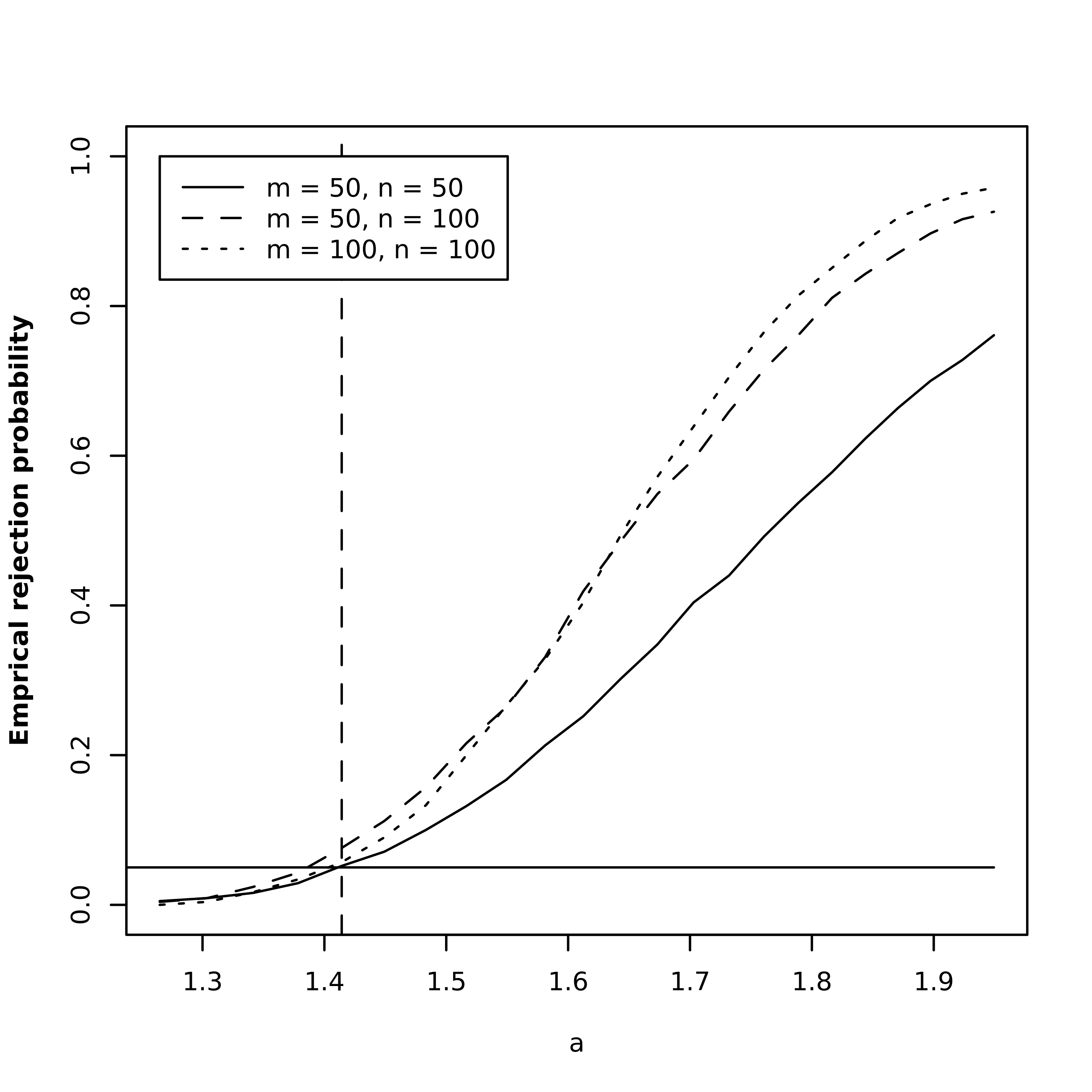
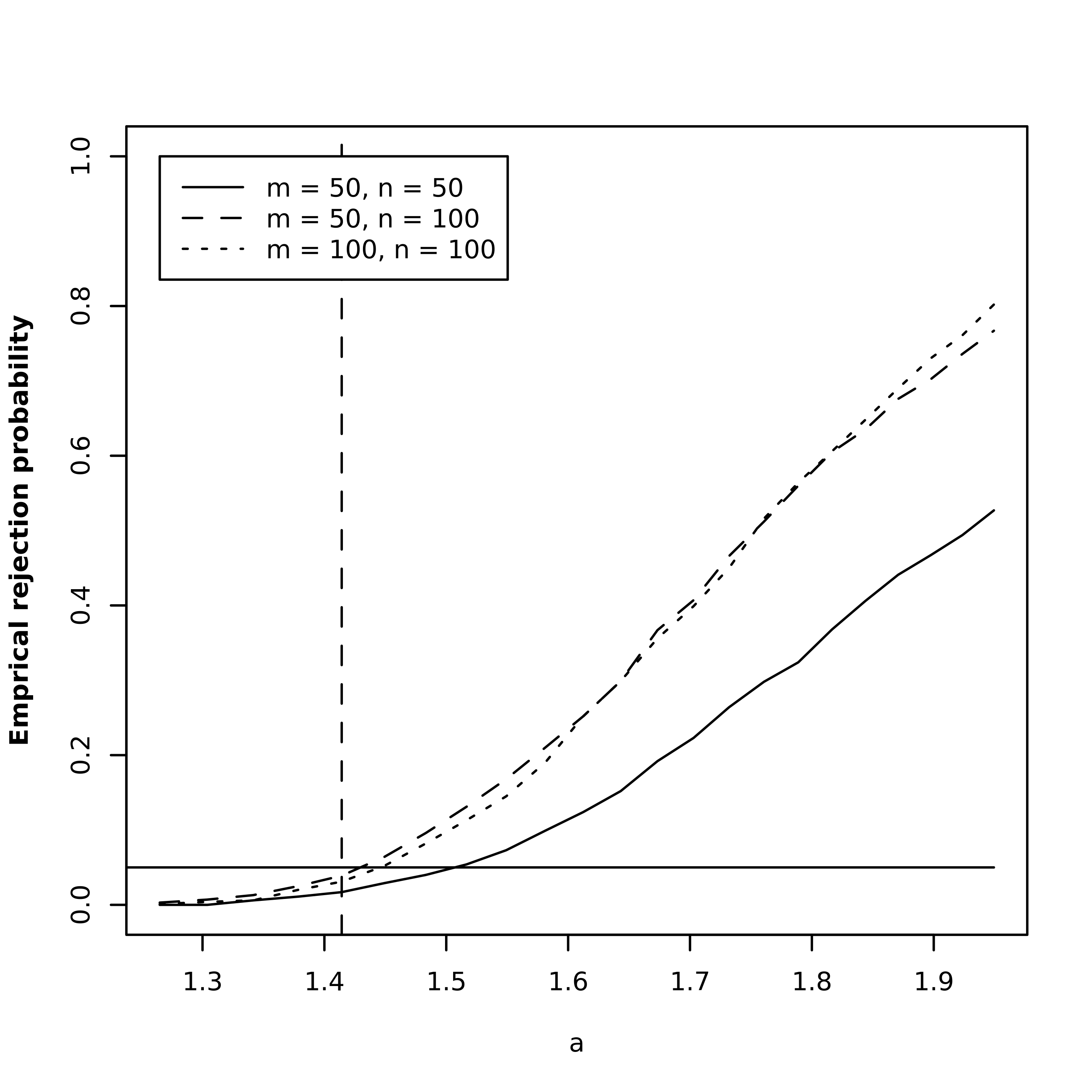
Figure 1: Simulated rejection probabilities of the test (3.19) for a non-relevant difference in the covariance operators. Left panel fMA(1) with threshold $\Delta=1+0.7^{2}$. Right panel non-Gaussian curves with threshold $\Delta=1$. The second sample is multiplied by $a$ for $a=\sqrt{1.6},\sqrt{1.7},\dots,\sqrt{3.8}$, and the vertical lines represent the boundary of the null hypotheses (i.e. $a=\sqrt{2}$).

5.1.2 Change point problem

Classical hypotheses:

We begin with a comparison of the test (4.12) for the classical hypotheses (3.4) with two procedures which were recently proposed by Sharipov and Wendler, (2019) and are based on the sup and $L^{2}$-norm of the CUSUM statistic. Following these authors we generate data from the model

(5.6) $$X_{n,i}(t)=\begin{cases}\varepsilon_{X,i}(t)\,,&i<k^{*}=\lfloor s^{*}n\rfloor+1\\ \varepsilon_{X,i}(t)(1+d_{1}+d_{2}(1+\sin(2\pi t)))\,,&i\geq k^{*}\end{cases}$$

where $\varepsilon_{X,1},\dots,\varepsilon_{X,n}$ are independent standard Brownian motions. A sample size of $n=100$ is considered and the true change point is defined by $k^{*}=51$. The empirical rejection probabilities of the three tests are displayed in Table 3. The level ($d_{1}=d_{2}=0$) is approximated very well by all procedures under consideration. Moreover, the test (4.12) proposed in this paper is at least competitive in all cases under consideration. In the case $d_{1}=0.4,d_{2}=0$ the procedures of Sharipov and Wendler, (2019) perform slightly better but whenever $d_{2}>0$, the new procedure shows the best performance.

$d_{1},\,d_{2}$	1%	5%	10%	$d_{1},\,d_{2}$	1%	5%	10%
0, 0	1.3	5.0	9.9	0.4, 0	19.3	44.5	61.0
	(0.4, 0.6)	(4.4, 4.7)	(10.0, 10.8)		(16.1, 19.8)	(46.8, 50.1)	(63.2, 65.4)
0.8, 0	60.0	88.4	95.2	0, 0.4	22.4	48.9	65.3
	(56.0, 58.8)	(88.0, 88.4)	(96.0, 95.5)		(9.8, 12.5)	(33.0, 38.6)	(49.4, 55.4)
0, 0.8	69.8	93.6	98.0	0.4, 0.4	63.4	89.3	95.8
	(45.8, 50.3)	(82.9, 85.8)	(93.8, 94.6)		(44.2, 49.1)	(81.1, 82.2)	(91.6, 92.1)

Table 3: Empirical rejection probabilities of the bootstrap test (4.12) for the classical hypotheses (3.4) of a structural break in the covariance operator. The numbers in the brackets display the empirical rejection probabilities of the test proposed in Sharipov and Wendler, (2019) based on the supremum type integral type CUSUM statistic (for $p=3$).

Next we provide a comparison with the procedure proposed by Stoehr et al., (2019). Following these authors, we simulate fAR(1) data where the errors (similar as in (5.2)) are defined by

$$e_{j}=\sum_{i=1}^{55}N_{i,j}\tilde{\nu}_{i}\,,\qquad j=1,\dots,n\,,$$

$\tilde{\nu}_{1},\dots,\tilde{\nu}_{55}$ denote the Fourier basis and the random coefficients $N_{1,j},N_{2,j},\dots,N_{55,j}$ are independent normally distributed with expectation zero and variance $\mbox{Var}(N_{i,j})=\sigma_{i}^{2}$ ($i=1,\ldots,55$; $j=1,\ldots,n$). The fAR(1) data are then defined by

(5.7) $$X_{n,j}=\Psi(X_{n,j-1})+e_{j}\,,\qquad j=1,\ldots,n\,,$$

where the linear operator $\Psi$ is represented by a $55\times 55$ matrix that is applied to the vector of the coefficients in the basis representation. Here the matrix with $0.4$ on the diagonal and $0.1$ on the superdiagonal and subdiagonal is chosen, such that the generated fAR(1) time series is stationary. For the alternative a change is inserted in the first $m$ leading eigendirections for $m=2,6,25$ by adding an additional normally distributed noise term with variance $\sigma_{\epsilon}^{2}/m$ for the observations $X_{n,j}$ for $j>\lfloor 0.5n\rfloor$. The following three settings are considered:

$$\text{Setting 1: }~{}\sigma_{i}=1~{}\text{ for }~{}i=1,\dots,8~{}\text{ and }~{}\sigma_{i}=0~{}\text{ for }~{}i=9,\dots,55,~{}~{}\sigma_{\epsilon}=1.5$$

$$\text{Setting 2: }~{}\sigma_{i}=3^{-i}~{}\text{ for }~{}i=1,\dots,55,~{}~{}\sigma_{\epsilon}=0.3$$

$$\text{Setting 3: }~{}\sigma_{i}=i^{-1}~{}\text{ for }~{}i=1,\dots,55,~{}~{}\sigma_{\epsilon}=1\,.$$

The empirical rejection probabilities of the test (4.12) with block length $l=6$ and the test based on dimension reduction developed in Stoehr et al., (2019) are displayed in Table 4. We observe that in all cases under consideration the procedure proposed here yields an improvement with respect to the power. Note that Stoehr et al., (2019) also considered test procedures based on fully functional and weighted functional statistics. As these methods considerably overestimate the test level (see Figure 2 in the same reference), these procedures are not included in the comparison.

$m$	Setting 1	Setting 2	Setting 3
0	4.7 (3.1)	8.1 (5.0)	3.9 (4.6)
2	37.2 (22.8)	92.5 (50.5)	86.2 (30.4)
6	81.1 (20.4)	99.9 (98.9)	99.9 (94.8)
25	100 (29.0)	100 (92.3)	100 (97.3)

Table 4: Empirical rejection probabilities (at level $5\%$) of the bootstrap test (4.12) and the dimension reduction approach proposed in Stoehr et al., (2019) (numbers in the brackets).

Relevant hypotheses:

We conclude this section investigating the finite sample properties of the test defined by (4.16) for the hypotheses (3.3) of a relevant change in the covariance operator. For this purpose we consider similar scenarios as in Section 5.1.1. In all cases, the location of the change is set to $s^{*}=0.5$ and the observations after the change point are multiplied by a constant $a$ such that (5.5) holds. For the estimation of the extremal sets, the parameter in (4.14) is set as $c_{n}=0.1\log(n)$.

In Table 5 empirical rejection probabilities are displayed for different processes at the boundary of the null hypothesis i.e. the observations after the change point are multiplied by $a=2$ and the threshold $\Delta$ is defined in each case such that $\|C_{1}-C_{2}\|_{\infty}=\Delta$. For fIID and non-Gaussian data the block length in (4.8) is set to $l=1$ and the threshold is given by $\Delta=a^{2}-1$. The fMA(1) and fMA(2) data are defined by (5.4) with $\kappa_{1}=0.7,\kappa_{2}=0$ and $\kappa_{1}=0.5,\kappa_{2}=0.3$, respectively. The threshold parameter is set to $\Delta=(a^{2}-1)(1+\kappa_{1}^{2}+\kappa_{2}^{2})$ in both cases and the block length in (4.8) is set to $l=2$ and $l=3$, respectively.

We observe that the nominal level is reasonably well approximated in most cases under consideration especially for the sample size $n=200$. Only in the non-Gaussian case, the nominal level is underestimated for the sample size $N=100$, but the approximation improves considerably for the sample size $N=200$.

In Table 6, we show the empirical rejection probabilities of the test (4.16) and also for the test developed in Dette et al., 2020b for scenarios in the interior of the null hypothesis of no relevant change point as well as under the alternative. We consider independent identically distributed Gaussian (fIID) and fMA(2) data and multiply the observations after the change point by different values $a=1.8,1.9,2,2.2,2.4,2.6$. In the fIID case the threshold parameter is given by $\Delta=3$ and in the fMA(2) case it is $\Delta=3\cdot(1+\kappa_{1}^{2}+\kappa_{2}^{2})$ (where still $\kappa_{1}=0.5,\kappa_{2}=0.3$). Consequently, the case $a=2$ always corresponds to the boundary of the null hypothesis, and the cases $a<2$ and $a>2$ represent the interior of the null hypothesis and alternative. Since the procedure developed by Dette et al., 2020b is based on a different metric, the threshold parameter $\Delta$ in the relevant hypotheses (1.2) is set to

$$\Delta=\int_{[0,1]}\int_{[0,1]}\{(1-2^{2})C_{1}(s,t)\}^{2}dsdt$$

for this test procedure. Consequently the boundary of the null hypothesis of no relevant change in the covariance operators (w.r.t. the corresponding metric) is also obtained for the factor $a=2$ for both data models.

We mention again that the nominal level at the boundary of the hypotheses is reasonably well approximated by the test (4.16) while the test procedure developed in Dette et al., 2020b is more conservative. In the interior of the null hypothesis $(a<2)$ the rejection probabilities of both tests are strictly smaller than the nominal level. This property is desirable as it means that the probability of a type I error is small in situations with a large deviation from the alternative. On the other hand, under the alternative the new test (4.16) has substantially more power than the test developed in Dette et al., 2020b .

	fIID			non-Gaussian			fMA(1)			fMA(2)
$n$	1%	5%	10%	1%	5%	10%	1%	5%	10%	1%	5%	10%
100	1.1	3.8	9.5	0	0.8	5.3	0.8	4.9	13.7	1.3	6.0	11.7
200	0.7	4.6	10.1	0.3	3.1	8.4	1.3	4.9	9.8	0.7	4.9	10.5

Table 5: Simulated level of the test (4.16) for the hypotheses defined by (3.3) at the boundary of the hypotheses, that is $\|C_{1}-C_{2}\|_{\infty}=\Delta$.

	fIID		fMA(2)
$a$	$n=100$	$n=200$	$n=100$	$n=200$
1.8	0.3 (0.4)	0 (0)	1.3 (0.1)	1.0 (0.1)
1.9	1.8 (0.9)	0.1 (0.5)	3.4 (0.4)	1.4 (0.4)
2.0	3.8 (2.3)	4.6 (3.2)	6.0 (1.0)	4.9 (1.4)
2.2	21.5 (9.8)	33.6 (25.4)	19.4 (6.2)	27.2 (11.1)
2.4	47.0 (23.3)	74.9 (51.2)	40.0 (15.6)	65.9 (31.2)
2.6	73.0 (37.9)	96.0 (70.6)	63.3 (26.5)	88.0 (49.7)

Table 6: Simulated rejection probabilities of the test (4.16) for the hypotheses (3.3) of a relevant change in the covariance operator considering fIID and fMA(2) data (level $5\%$). The cases $a<2,a=2$ and $a>2$ correspond to the interior, boundary of the null hypothesis and to the alternative. The numbers in brackets represent the empirical rejection probabilities of the procedure developed in Dette et al., 2020b .

5.2 Data Example

Similar as Fremdt et al., (2013) and Paparoditis and Sapatinas, (2016) we consider egg-laying curves of medflies (Mediterranean fruit flies, Ceratitis capitata). The original data consists of the number of eggs which were laid on each day during the lifetime of $1000$ female medflies and a detailed description of the experiment can be found in Carey et al., (1998). Only medflies which lived at least $34$ days are considered and split into two samples, the medflies which lived at most $43$ days and those which lived at least $44$ days. A Fourier basis consisting of $49$ basis functions is used to transform the discrete observations to functional data $(X_{j}\colon j=1,\dots,256)$ and $(Y_{j}\colon j=1,\dots,278)$. The expressions $X_{i}(t)$ and $Y_{j}(t)$ denote the number of eggs which were laid on day $\lfloor 30t\rfloor$ by the $i$th short-lived and the $j$th long-lived medfly relative to the total number of eggs laid in the whole lifetime of the $i$th short-lived and the $j$th long-lived medfly, respectively ($t\in[0,1],i=1,\dots,256,j=1,\dots,278$). First, the test (3.14) is used to study the classical hypotheses in (3.4). The window parameters in (3.12) are set to $l_{1}=l_{2}=1$ since the egg-laying curves corresponding to the different medflies can be regarded as independent. For the calculation of critical values, $200$ bootstrap samples are generated. The classical null hypothesis of equal covariance operators is then rejected at level $5\%$ and can not be rejected at level $1\%$. The outcome when using the procedure developed in Fremdt et al., (2013) depends on the choice of the number of considered functional principal components $p$ and the procedure developed in Paparoditis and Sapatinas, (2016) yields a $p$-value of $0.3\%$ (see Table 3 in Paparoditis and Sapatinas, (2016)). In Table 7 the empirical rejection probabilities of the test (3.19) are displayed for the relevant hypotheses in (3.3) for different choices of the threshold parameter $\Delta$. It can be seen that even for $\Delta=0.0003$ i.e. when a maximal deviation of only $0.0003$ is tolerated, the null hypothesis of no relevant difference between the covariance operators can not be rejected at all considered test levels. For $\Delta=0.0002$ the null can be rejected at level $10\%$ and for $\Delta=0.0001$ also at level $5\%$. Although the classical null hypothesis of equal covariance operators is rejected at level $5\%$, these results may raise the question if the detected difference is really of practical relevance.

$\Delta$	1%	5%	10%
0.0001	FALSE	TRUE	TRUE
0.0002	FALSE	FALSE	TRUE
0.0003	FALSE	FALSE	FALSE

Table 7: Summary of the outcome of the test (3.19) for the relevant hypotheses (3.3) for different values of $\Delta$ for the relative egg-laying curves of medflies. The label TRUE means that the null hypothesis is rejected and the label FALSE means that the null hypothesis is not rejected.

6 Appendix: Proofs of main results

6.1 Proof of Theorem 2.1

We apply the central limit theorem as formulated in Theorem 2.1 in Dette et al., 2020a to the sequence of $C(T^{2})$-valued random variables $((Z_{j}-\mu)^{\check{\otimes}2})_{j\in\mathbb{N}}=(\eta_{j}^{\check{\otimes}2})_{j\in\mathbb{N}}$.

It can be easily seen that conditions (A1), (A2) and (A4) in this reference are satisfied. In order to see that the remaining condition (A3) also holds, we use the triangle inequality and Assumption 2.1 of the present work to obtain, for any $j\in\mathbb{N}$ and $s,t,s^{\prime},t^{\prime}\in T$,

$$|\eta_{j}(s)\eta_{j}(t)-\eta_{j}(s^{\prime})\eta_{j}(t^{\prime})| \leq|\eta_{j}(s)(\eta_{j}(t)-\eta_{j}(t^{\prime}))|+|\eta_{j}(t^{\prime})(\eta_{j}(s)-\eta_{j}(s^{\prime}))|$$

$$\leq\|\eta_{j}\|_{\infty}\,\big{(}|\eta_{j}(t)-\eta_{j}(t^{\prime})|+|\eta_{j}(s)-\eta_{j}(s^{\prime})|\big{)}$$

$$\leq\|\eta_{j}\|_{\infty}\,M\,\big{(}\rho(t,t^{\prime})+\rho(s,s^{\prime})\big{)}$$

$$\lesssim\|\eta_{j}\|_{\infty}\,M\,\rho_{\max}\big{(}(t,s),(t^{\prime},s^{\prime})\big{)}$$

where $\mathbb{E}\big{[}(\|\eta_{j}\|_{\infty}\,M)^{J}\big{]}\leq\tilde{K}<\infty$ by (A3). Now observe that

$$\frac{1}{\sqrt{n}}\sum_{j=1}^{n}(Z_{j}-\bar{Z}_{n})^{\check{\otimes}2}=\frac{1}{\sqrt{n}}\sum_{j=1}^{n}\eta_{j}^{\check{\otimes}2}-\frac{1}{\sqrt{n}}\bigg{(}\frac{1}{\sqrt{n}}\sum_{j=1}^{n}\eta_{j}\bigg{)}^{\check{\otimes}2}=\frac{1}{\sqrt{n}}\sum_{j=1}^{n}\eta_{j}^{\check{\otimes}2}+o_{\mathbb{P}}(1)$$

which yields the claim since Theorem 2.1 in Dette et al., 2020a can be applied to the sequence $(\eta_{j}^{\check{\otimes}2})_{j\in\mathbb{N}}$ as shown above.

6.2 Proof of Proposition 3.1

As the samples are independent, it directly follows from Theorem 2.1 that

$$\sqrt{m+n} \bigg{(}\frac{1}{m}\sum_{j=1}^{m}(\tilde{X}_{m,j}^{\check{\otimes}2}-C_{1}),\,\frac{1}{n}\sum_{j=1}^{n}(\tilde{Y}_{n,j}^{\check{\otimes}2}-C_{2})\bigg{)}$$

$$=\sqrt{m+n}\bigg{(}\frac{1}{m}\sum_{j=1}^{m}(\eta_{1,j}^{\check{\otimes}2}-C_{1}),\,\frac{1}{n}\sum_{j=1}^{n}(\eta_{2,j}^{\check{\otimes}2}-C_{2})\bigg{)}+o_{\mathbb{P}}(1)\rightsquigarrow\bigg{(}\frac{1}{\sqrt{\lambda}}~{}Z_{1},\frac{1}{\sqrt{1-\lambda}}~{}Z_{2}\bigg{)}$$

in $C([0,1]^{2})^{2}$ as $m,n\to\infty$, where $Z_{1}$ and $Z_{2}$ are independent, centred Gaussian processes defined by their long-run covariance operators (3.8) and (3.9). By the continuous mapping theorem it follows that

(6.1) $$Z_{m,n}=\sqrt{m+n}\,\bigg{(}\frac{1}{m}\sum_{j=1}^{m}\tilde{X}_{m,j}^{\check{\otimes}2}-\,\frac{1}{n}\sum_{j=1}^{n}\tilde{Y}_{n,j}^{\check{\otimes}2}-(C_{1}-C_{2})\bigg{)}\rightsquigarrow Z$$

in $C([0,1]^{2})$ as $m,n\to\infty$, where $Z$ is again a centred Gaussian process with covariance operator (3.7).

If $d_{\infty}=0$, the convergence in (6.1) together with the continuous mapping yield (3.6). If $d_{\infty}>0$, the asymptotic distribution of $\hat{d}_{\infty}$ can be deduced from Theorem B.1 in the online supplement of Dette et al., 2020a or alternatively from the results in Cárcamo et al., (2020).

6.3 Proof of Theorem 3.1 and 3.2

Proof of Theorem  3.1. Using similar arguments as in the proof of Theorem 2.1, it follows that the process $\hat{B}^{(r)}_{m,n}$ in (3.12) admits the stochastic expansion

$$\hat{B}^{(r)}_{m,n}=\sqrt{n+m}\bigg{\{} \frac{1}{m}\sum_{k=1}^{m-l_{1}+1}\frac{1}{\sqrt{l_{1}}}\bigg{(}\sum_{j=k}^{k+l_{1}-1}\eta_{1,j}^{\check{\otimes}2}-\frac{l_{1}}{m}\sum_{i=1}^{m}\eta_{1,j}^{\check{\otimes}2}\bigg{)}\xi_{k}^{(r)}$$

$$- \frac{1}{n}\sum_{k=1}^{n-l_{2}+1}\frac{1}{\sqrt{l_{2}}}\bigg{(}\sum_{j=k}^{k+l_{2}-1}\eta_{2,j}^{\check{\otimes}2}-\frac{l_{2}}{n}\sum_{i=1}^{n}\eta_{2,j}^{\check{\otimes}2}\bigg{)}\zeta_{k}^{(r)}\bigg{\}}+o_{\mathbb{P}}(1)\,,$$

and the sequences $(\eta_{1,j}^{\check{\otimes}2})_{j\in\mathbb{N}}$ and $(\eta_{2,j}^{\check{\otimes}2})_{j\in\mathbb{N}}$ satisfy Assumption 2.1 in Dette et al., 2020a . Thus, similar arguments as in the proof of Theorem 3.3 in the same reference yield

(6.2) $$\big{(}Z_{m,n},\hat{B}_{m,n}^{(1)},\dots,\hat{B}_{m,n}^{(R)}\big{)}\rightsquigarrow(Z,Z^{(1)},\dots,Z^{(R)})$$

in $C([0,1]^{2})^{R+1}$ as $m,n\to\infty$ where the process $Z_{m,n}$ is defined in (6.1) and the random functions $Z^{(1)},\dots,Z^{(R)}$ are independent copies of $Z$ which is also defined in (6.1).

If $d_{\infty}=0$, the continuous mapping theorem implies

(6.3) $$\big{(}\sqrt{m+n}\,\hat{d}_{\infty},~{}T_{m,n}^{(1)},\dots,T_{m,n}^{(R)}\big{)}\stackrel{{\scriptstyle\mathcal{D}}}{{\longrightarrow}}(T,~{}T^{(1)},\dots,T^{(R)})$$

in $\mathbb{R}^{R+1}$ as $m,n\to\infty$ where the statistic $\hat{d}_{\infty}$ is defined by (3.5), the bootstrap statistics $T_{m,n}^{(1)},\dots,T_{m,n}^{(R)}$ are defined by (3.13) and the random variables $T^{(1)},\dots,T^{(R)}$ are independent copies of $T$ which is defined by (3.6). Now, Lemma 4.2 in Bücher and Kojadinovic, (2019) directly implies (3.15), that is

$$\lim_{m,n,R\to\infty}\mathbb{P}\bigg{(}\hat{d}_{\infty}>\frac{T_{m,n}^{\{\lfloor R(1-\alpha)\rfloor\}}}{\sqrt{m+n}}\bigg{)}=\alpha\,.$$

For the application of this result, it is required that the distribution of the random variable $T$ has a continuous distribution function, which follows from Gaenssler et al., (2007). In order to show the consistency of test (3.14) in the case $d_{\infty}>0$, write

$$\mathbb{P}\bigg{(}\hat{d}_{\infty}>\frac{T_{m,n}^{\{\lfloor R(1-\alpha)\rfloor\}}}{\sqrt{m+n}}\bigg{)} =\mathbb{P}\big{(}\sqrt{m+n}\,(\hat{d}_{\infty}-d_{\infty})+\sqrt{m+n}\,d_{\infty}>T_{m,n}^{\{\lfloor R(1-\alpha)\rfloor\}}\big{)}$$

and note that, given (6.3) and (3.10), the assertion in (3.16) follows by simple arguments.

Proof of Theorem 3.2. First note that the same arguments as in the proof of Theorem 3.6 in Dette et al., 2020a show that the estimators of the extremal sets defined by (3.17) are consistent that is

$$d_{H}(\hat{\mathcal{E}}_{m,n}^{\pm},\mathcal{E}^{\pm})\xrightarrow[m,n\to\infty]{\mathbb{P}}0\,,$$

where $d_{H}$ denotes the Hausdorff distance. Thus, given the convergence in (6.2), the arguments in the proof of Theorem 3.7 in the same reference yield

(6.4) $$\big{(}\sqrt{n+m}~{}(\hat{d}_{\infty}-d_{\infty}),~{}K_{m,n}^{(1)},\dots,K_{m,n}^{(R)}\big{)}\stackrel{{\scriptstyle\mathcal{D}}}{{\longrightarrow}}(T(\mathcal{E}),~{}T^{(1)}(\mathcal{E}),\dots,T^{(R)}(\mathcal{E}))$$

in $\mathbb{R}^{R+1}$ as $m,n\to\infty$ where the statistic $\hat{d}_{\infty}$ is defined by (3.5), the bootstrap statistics $K_{m,n}^{(1)},\dots,K_{m,n}^{(R)}$ are defined by (3.18) and the random variables $T^{(1)}(\cal E),\dots,T^{(R)}(\cal E)$ are independent copies of $T(\mathcal{E})$ which is defined by (3.10). Note that this convergence holds true under the null and the alternative hypothesis.

If $\Delta=d_{\infty}$, Lemma 4.2 in Bücher and Kojadinovic, (2019) directly implies (3.20) and again the results in Gaenssler et al., (2007) ensure that the limit $T(\mathcal{E})$ has a continuous distribution function.

If $\Delta\neq d_{\infty}$, write

$$\mathbb{P}\bigg{(}\hat{d}_{\infty}>\Delta+\frac{K_{m,n}^{\{\lfloor R(1-\alpha)\rfloor\}}}{\sqrt{n+m}}\bigg{)}=\mathbb{P}\big{(}\sqrt{m+n}\,(\hat{d}_{\infty}-d_{\infty})+\sqrt{m+n}\,(d_{\infty}-\Delta)>K_{m,n}^{\{\lfloor R(1-\alpha)\rfloor\}}\big{)}\,.$$

Then it follows from (6.4) and simple arguments that, for any $R\in\mathbb{N}$,

$$\lim_{m,n\to\infty}\mathbb{P}\bigg{(}\hat{d}_{\infty}>\Delta+\frac{K_{m,n}^{\{\lfloor R(1-\alpha)\rfloor\}}}{\sqrt{n+m}}\bigg{)}=0\quad\text{and}\quad\liminf_{m,n\to\infty}\mathbb{P}\bigg{(}\hat{d}_{\infty}>\Delta+\frac{K_{m,n}^{\{\lfloor R(1-\alpha)\rfloor\}}}{\sqrt{n+m}}\bigg{)}=1$$

if $\Delta>d_{\infty}$ and $\Delta<d_{\infty}$, respectively. This proves the remaining assertions of Theorem 3.2.

6.4 Proof of Proposition 4.1

Let $C_{n,j}$ denote the covariance operator of $X_{n,j}$ defined by $C_{n,j}(s,t)=\mbox{Cov}(X_{n,j}(s),X_{n,j}(t))$ and consider the sequential process

$$\hat{\mathbb{V}}_{n}(s) =\frac{1}{\sqrt{n}}\sum^{\lfloor sn\rfloor}_{j=1}(\tilde{X}_{n,j}^{\check{\otimes}2}-C_{n,j})+\sqrt{n}\Big{(}s\,-\frac{\lfloor sn\rfloor}{n}\Big{)}\big{(}\tilde{X}_{n,\lfloor sn\rfloor+1}^{\check{\otimes}2}-C_{n,\lfloor sn\rfloor+1}\big{)}\,$$

$$=\frac{1}{\sqrt{n}}\sum^{\lfloor sn\rfloor}_{j=1}(\tilde{\eta}_{n,j}^{\check{\otimes}2}-C_{n,j})+\sqrt{n}\Big{(}s\,-\frac{\lfloor sn\rfloor}{n}\Big{)}\big{(}\tilde{\eta}_{n,\lfloor sn\rfloor+1}^{\check{\otimes}2}-C_{n,\lfloor sn\rfloor+1}\big{)}+o_{\mathbb{P}}(1)$$

which is an element of $C([0,1],C([0,1]^{2}))$. Note that $\{\hat{\mathbb{V}}_{n}(s)\}_{s\in[0,1]}$ can equivalently be regarded as an element of $C([0,1]^{3})$ and we have the representation

(6.5) $$\hat{\mathbb{V}}_{n}=\tilde{\mathbb{V}}_{1,n}+\tilde{\mathbb{V}}_{2,n}\,,$$

where the processes $\tilde{\mathbb{V}}_{1,n},\tilde{\mathbb{V}}_{2,n}\in C([0,1]^{3})$ are defined by

$$\tilde{\mathbb{V}}_{1,n}(s,t,u) =\,\hat{\mathbb{V}}_{1,n}(s,t,u)\mathds{1}\{\lfloor sn\rfloor<\lfloor s^{*}n\rfloor\}+\hat{\mathbb{V}}_{1,n}(\lfloor s^{*}n\rfloor/n,t,u)\mathds{1}\{\lfloor sn\rfloor\geq\lfloor s^{*}n\rfloor\}$$

$$\tilde{\mathbb{V}}_{2,n}(s,t,u) =\,(\hat{\mathbb{V}}_{2,n}(s,t,u)-\hat{\mathbb{V}}_{2,n}(\lfloor s^{*}n\rfloor/n,t,u))\mathds{1}\{\lfloor sn\rfloor\geq\lfloor s^{*}n\rfloor\}$$

($s,t,u\in[0,1]$) and

$$\hat{\mathbb{V}}_{l,n}(s)=\frac{1}{\sqrt{n}}\sum^{\lfloor sn\rfloor}_{j=1}(\eta_{l,j}^{\check{\otimes}2}-C_{l})+\sqrt{n}\Big{(}s\,-\frac{\lfloor sn\rfloor}{n}\Big{)}\big{(}\eta_{l,\lfloor sn\rfloor+1}^{\check{\otimes}2}-C_{l}\big{)}\quad\quad(l=1,2)\,.$$

Recall the definition of the array ($\tilde{\eta}_{n,j}\colon n\in\mathbb{N},j=1,\dots,n$) in (4.1). By Theorem 2.2 in Dette et al., 2020a it follows that

$$\hat{\mathbb{V}}_{l,n}\rightsquigarrow\mathbb{V}_{l}\quad\quad(l=1,2)$$

in $C([0,1]^{3})$, where $\mathbb{V}_{l}$ is a centred Gaussian measure on $C([0,1]^{3})$ characterized by the covariance operator

$$\mbox{Cov}\big{(}\mathbb{V}_{l}(s,t,u),\mathbb{V}_{l}(s^{\prime},t^{\prime},u^{\prime})\big{)} =(s\wedge s^{\prime})\,\mathbb{C}_{l}((t,u),(t^{\prime},u^{\prime})),\qquad l=1,2$$

and the long-run covariance operator $\mathbb{C}_{l}$ is defined in (4.6). From the continuous mapping theorem we obtain

(6.6) $$\tilde{\mathbb{V}}_{l,n}\rightsquigarrow\tilde{\mathbb{V}}_{l}\quad\quad(l=1,2)$$

in $C([0,1]^{3})$, where $\tilde{\mathbb{V}}_{1},\tilde{\mathbb{V}}_{2}$ are centred Gaussian measures on $C([0,1]^{3})$ characterized by

$$\tilde{\mathbb{V}}_{1}(s,t,u)=\mathbb{V}_{1}(s\wedge s^{*},t,u)\,,\quad\tilde{\mathbb{V}}_{2}(s,t,u)=(\mathbb{V}_{2}(s,t,u)-\mathbb{V}_{2}(s^{*},t,u))\mathds{1}\{s\geq s^{*}\}$$

with covariance operators

$$\mbox{Cov}\big{(}\tilde{\mathbb{V}}_{1}(s,t,u),\tilde{\mathbb{V}}_{1}(s^{\prime},t^{\prime},u^{\prime})\big{)} =(s\wedge s^{\prime}\wedge s^{*})\,\mathbb{C}_{1}((t,u),(t^{\prime},u^{\prime}))$$

$$\mbox{Cov}\big{(}\tilde{\mathbb{V}}_{2}(s,t,u),\tilde{\mathbb{V}}_{2}(s^{\prime},t^{\prime},u^{\prime})\big{)} =(s\wedge s^{\prime}-s^{*})_{+}\,\mathbb{C}_{2}((t,u),(t^{\prime},u^{\prime}))\,.$$

In the following we will show the weak convergence

(6.7) $$\hat{\mathbb{V}}_{n}\rightsquigarrow\mathbb{V}$$

in $C([0,1]^{3})$ as $n\to\infty$, where $\mathbb{V}\in C([0,1]^{3})$ is a centred Gaussian random variable characterized by its covariance operator

$$\mbox{Cov}(\mathbb{V}(s,t,u),\mathbb{V}(s^{\prime},t^{\prime},u^{\prime}))=(s\wedge s^{\prime}\wedge s^{*})\,\mathbb{C}_{1}((t,u),(t^{\prime},u^{\prime}))+(s\wedge s^{\prime}-s^{*})_{+}\,\mathbb{C}_{2}((t,u),(t^{\prime},u^{\prime}))$$

and the long-run covariance operators $\mathbb{C}_{1},\mathbb{C}_{2}$ are defined by (4.6). The convergence in (6.6) implies that the processes $\tilde{\mathbb{V}}_{1,n},\tilde{\mathbb{V}}_{2,n}$ are asymptotically tight and the representation in (6.5) yields that $\hat{\mathbb{V}}_{n}$ is asymptotically tight as well (see Section 1.5 in Van der Vaart and Wellner,, 1996). In order to prove the convergence in (6.7) it consequently remains to show the convergence of the finite dimensional distributions. For this, we utilize the Crámer-Wold device and show that

$$\tilde{Z}_{n}=\sum_{j=1}^{q}c_{j}\hat{\mathbb{V}}_{n}(s_{j},t_{j},u_{j}) =\sum_{j=1}^{q}c_{j}\big{\{}\tilde{\mathbb{V}}_{1,n}(s_{j},t_{j},u_{j})+\tilde{\mathbb{V}}_{2,n}(s_{j},t_{j},u_{j})\big{\}}$$

$$\stackrel{{\scriptstyle\cal D}}{{\longrightarrow}}\tilde{Z}=\sum_{j=1}^{q}c_{j}\mathbb{V}(s_{j},t_{j},u_{j})$$

for any $(s_{1},t_{1},u_{1}),\dots,(s_{q},t_{q},u_{q})\in[0,1]^{3}$, $c_{1},\dots,c_{q}\in\mathbb{R}$ and $q\in\mathbb{N}$. Asymptotic normality of $\tilde{Z}_{n}$ can be proved by the same arguments as in the proof of Theorem 2.1 in Dette et al., 2020a and it remains to show that the variance of the random variable $\tilde{Z}_{n}$ converges to the variance of $\tilde{Z}$. Using (3.17) in Dehling and Philipp, (2002) and assumptions (A2) and (A4) we obtain for any $(s,t,u),(s^{\prime},t^{\prime},u^{\prime})\in[0,1]^{3}$

(6.8) $$\begin{split}&\mbox{Cov}(\tilde{\mathbb{V}}_{1,n}(s,t,u),\tilde{\mathbb{V}}_{2,n}(s^{\prime},t^{\prime},u^{\prime}))\\ &=\frac{1}{n}\sum^{\lfloor(s\wedge s^{*})n\rfloor}_{j=1}\sum^{\lfloor s^{\prime}n\rfloor}_{i=\lfloor s^{*}n\rfloor+1}\mbox{Cov}(\tilde{\eta}_{n,j}^{\check{\otimes}2}(t,u),\tilde{\eta}_{n,i}^{\check{\otimes}2}(t^{\prime},u^{\prime}))+o(1)\\ &\lesssim\frac{1}{n}\sum^{\lfloor(s\wedge s^{*})n\rfloor}_{j=1}\sum^{\lfloor s^{\prime}n\rfloor}_{i=\lfloor s^{*}n\rfloor+1}\|\tilde{\eta}_{n,j}^{\check{\otimes}2}(t,u)\|_{2}\,\|\tilde{\eta}_{n,i}^{\check{\otimes}2}(t^{\prime},u^{\prime})\|_{2}\,\varphi(i-j)^{1/2}+o(1)\\ &\lesssim\frac{1}{n}\sum^{\lfloor(s\wedge s^{*})n\rfloor}_{j=1}\sum^{\lfloor s^{\prime}n\rfloor}_{i=\lfloor s^{*}n\rfloor+1}\varphi(i-j)^{1/2}+o(1)\\ &\lesssim\frac{1}{n}\sum^{\lfloor s^{\prime}n\rfloor-1}_{i=1}i\varphi(i)^{1/2}+o(1)\stackrel{{\scriptstyle[}}{{n}}\to\infty]{}{\longrightarrow}0\,,\end{split}$$

where the symbol “$\lesssim$” means less or equal up to a constant independent of $n$, and $\|X\|_{2}=\mathbb{E}[X^{2}]^{1/2}$ denotes the $L^{2}$-norm of a real valued random variable $X$ (also note that we implicitly assume $\sum_{i=j}^{k}a_{i}=0$ if $k<j$). Furthermore, assuming without loss of generality that $s\leq s^{\prime}$, we have

$$\mbox{Cov}(\tilde{\mathbb{V}}_{1,n}(s,t,u),\tilde{\mathbb{V}}_{1,n}(s^{\prime},t^{\prime},u^{\prime}))$$

$$=\frac{1}{n}\sum^{\lfloor(s\wedge s^{*})n\rfloor}_{j=1}\sum^{\lfloor(s^{\prime}\wedge s^{*})n\rfloor}_{i=1}\mbox{Cov}(\eta_{1,j}^{\check{\otimes}2}(t,u),\eta_{1,i}^{\check{\otimes}2}(t^{\prime},u^{\prime}))+o(1)$$

$$=\frac{1}{n}\sum^{\lfloor(s\wedge s^{*})n\rfloor}_{j=1}\bigg{(}\sum^{\lfloor(s\wedge s^{*})n\rfloor}_{i=1}+\sum^{\lfloor(s^{\prime}\wedge s^{*})n\rfloor}_{i=\lfloor(s\wedge s^{*})n\rfloor+1}\bigg{)}\mbox{Cov}(\eta_{1,j}^{\check{\otimes}2}(t,u),\eta_{1,i}^{\check{\otimes}2}(t^{\prime},u^{\prime}))+o(1)$$

$$=\frac{1}{n}\sum^{\lfloor(s\wedge s^{*})n\rfloor}_{j=1}\sum^{\lfloor(s\wedge s^{*})n\rfloor}_{i=1}\mbox{Cov}(\eta_{1,j}^{\check{\otimes}2}(t,u),\eta_{1,i}^{\check{\otimes}2}(t^{\prime},u^{\prime}))+o(1)\,,$$

where the last equality follows by the same arguments as used in (6.8). For the remaining expression we use the dominated convergence theorem to obtain

$$\frac{1}{n}\sum^{\lfloor(s\wedge s^{*})n\rfloor}_{j=1}\sum^{\lfloor(s\wedge s^{*})n\rfloor}_{i=1}\mbox{Cov}(\eta_{1,j}^{\check{\otimes}2}(t,u),\eta_{1,i}^{\check{\otimes}2}(t^{\prime},u^{\prime}))$$

$$=\sum^{\lfloor(s\wedge s^{*})n\rfloor-1}_{i=-(\lfloor(s\wedge s^{*})n\rfloor-1)}\frac{\lfloor(s\wedge s^{*})n\rfloor-|i|}{n}\,\mbox{Cov}(\eta_{1,0}^{\check{\otimes}2}(t,u),\eta_{1,i}^{\check{\otimes}2}(t^{\prime},u^{\prime}))\stackrel{{\scriptstyle[}}{{n}}\to\infty]{}{\longrightarrow}(s\wedge s^{*})\,\mathbb{C}_{1}((t,u),(t^{\prime},u^{\prime}))$$

which means that for any $(s,t,u),(s^{\prime},t^{\prime},u^{\prime})\in[0,1]^{3}$

$$\mbox{Cov}(\tilde{\mathbb{V}}_{1,n}(s,t,u),\tilde{\mathbb{V}}_{1,n}(s^{\prime},t^{\prime},u^{\prime}))\stackrel{{\scriptstyle[}}{{n}}\to\infty]{}{\longrightarrow}(s\wedge s^{\prime}\wedge s^{*})\,\mathbb{C}_{1}((t,u),(t^{\prime},u^{\prime}))\,.$$

By similar arguments we obtain

$$\mbox{Cov}(\tilde{\mathbb{V}}_{2,n}(s,t,u),\tilde{\mathbb{V}}_{2,n}(s^{\prime},t^{\prime},u^{\prime}))\stackrel{{\scriptstyle[}}{{n}}\to\infty]{}{\longrightarrow}(s\wedge s^{\prime}-s^{*})_{+}\,\mathbb{C}_{2}((t,u),(t^{\prime},u^{\prime}))$$

and therefore we have

$$\mbox{Var}(\tilde{Z}_{n}) =\sum_{j=1}^{q}\sum_{j^{\prime}=1}^{q}c_{j}c_{j^{\prime}}\mbox{Cov}(\hat{\mathbb{V}}_{n}(s_{j},t_{j},u_{j}),\hat{\mathbb{V}}_{n}(s_{j^{\prime}},t_{j^{\prime}},u_{j^{\prime}}))$$

$$=\sum_{j=1}^{q}\sum_{j^{\prime}=1}^{q}c_{j}c_{j^{\prime}}\big{\{}\mbox{Cov}(\tilde{\mathbb{V}}_{1,n}(s_{j},t_{j},u_{j}),\tilde{\mathbb{V}}_{1,n}(s_{j^{\prime}},t_{j^{\prime}},u_{j^{\prime}}))$$

$$\hskip 70.0pt+\mbox{Cov}(\tilde{\mathbb{V}}_{2,n}(s_{j},t_{j},u_{j}),\tilde{\mathbb{V}}_{2,n}(s_{j^{\prime}},t_{j^{\prime}},u_{j^{\prime}}))\big{\}}+o(1)$$

$$\stackrel{{\scriptstyle[}}{{n}}\to\infty]{}{\longrightarrow}\sum_{j=1}^{q}\sum_{j^{\prime}=1}^{q}c_{j}c_{j^{\prime}}\mbox{Cov}(\mathbb{V}(s_{j},t_{j},u_{j}),\mathbb{V}(s_{j^{\prime}},t_{j^{\prime}},u_{j^{\prime}}))=\mbox{Var}(\tilde{Z})$$

which finally proves (6.7).

Next we define the $C([0,1]^{3})$-valued process

(6.9) $$\hat{\mathbb{W}}_{n}(s,t,u)=\hat{\mathbb{V}}_{n}(s,t,u)-s\hat{\mathbb{V}}_{n}(1,t,u)\,,\qquad s,t,u\in[0,1]\,,$$

then the convergence in (6.7) and the continuous mapping theorem yield

(6.10) $$\hat{\mathbb{W}}_{n}\rightsquigarrow\mathbb{W}$$

in $C([0,1]^{3})$, where $\mathbb{W}$ is centred Gaussian defined by $\mathbb{W}(s,t,u)=\mathbb{V}(s,t,u)-s\mathbb{V}(1,t,u)$ with covariance operator given by (4.5). Finally, recall the definition of the process $(\hat{\mathbb{U}}_{n}\colon n\in\mathbb{N})$ in (4.2) and note that, in contrast to $\hat{\mathbb{W}}_{n}$, this process is not centred. Consequently, if $d_{\infty}=0$, we have $\sqrt{n}\,\mathbb{U}_{n}=\hat{\mathbb{W}}_{n}$ and the convergence in (6.10) and the continuous mapping theorem directly yield (4.4).

If $d_{\infty}>0$ assertion (4.7) is a consequence of the weak convergence in (6.10) and Theorem B.1 in the online supplement of Dette et al., 2020a and also of the results in Cárcamo et al., (2020).

6.5 Proof of Theorem  4.1 and 4.2

Proof of Theorem 4.1. It can be shown that the bootstrap processes in (4.8) can be written

$$\begin{split}\hat{B}_{n}^{(r)}(s,t,u)=&\frac{1}{\sqrt{n}}\sum_{k=1}^{\lfloor sn\rfloor}\frac{1}{\sqrt{l}}\Big{(}\sum_{j=k}^{k+l-1}\tilde{Y}_{n,j}(t,u)-\frac{l}{n}\sum_{j=1}^{n}\tilde{Y}_{n,j}(t,u)\Big{)}\xi_{k}^{(r)}\\ &+\sqrt{n}\Big{(}s-\frac{\lfloor sn\rfloor}{n}\Big{)}\frac{1}{\sqrt{l}}\Big{(}\sum_{j=\lfloor sn\rfloor+1}^{\lfloor sn\rfloor+l}\tilde{Y}_{n,j}(t,u)-\frac{l}{n}\sum_{j=1}^{n}\tilde{Y}_{n,j}(t,u)\Big{)}\xi_{\lfloor sn\rfloor+1}^{(r)}+o_{\mathbb{P}}(1)\end{split}$$

for $r=1,\dots,R$ where

$$\tilde{Y}_{n,j}=\tilde{\eta}_{n,j}^{\check{\otimes}2}(t,u)-(\hat{C}_{2}-\hat{C}_{1})\mathds{1}\{j>\lfloor\hat{s}n\rfloor\}$$

for $j=1,\dots,n$ ($n\in\mathbb{N}$) and the array $(\tilde{\eta}_{n,j}^{\check{\otimes}2}\,\colon n\in\mathbb{N},~{}j=1,\dots,n)$ satisfies (A1), (A3) and (A4) of Assumption 2.1 in Dette et al., 2020a . The convergence in (6.10) and similar arguments as in the proof of Theorem 4.3 in the same reference then imply

(6.11) $$\big{(}\hat{\mathbb{W}}_{n},\hat{\mathbb{W}}_{n}^{(1)},\dots,\hat{\mathbb{W}}_{n}^{(R)}\big{)}\rightsquigarrow(\mathbb{W},\mathbb{W}^{(1)},\dots,\mathbb{W}^{(R)})$$

in $C([0,1]^{3})^{R+1}$ as $n\to\infty$ where the process $\hat{\mathbb{W}}_{n}$ is defined by (6.9), the bootstrap counterparts $\hat{\mathbb{W}}_{n}^{(1)},\dots,\hat{\mathbb{W}}_{n}^{(R)}$ are defined by (4.10) and the random variables $\mathbb{W}^{(1)},\dots,\mathbb{W}^{(R)}$ are independent copies of $\mathbb{W}$ which is defined by its covariance operator (4.5).

If $d_{\infty}=0$, the continuous mapping theorem directly implies

$$\big{(}\hat{\mathbb{M}}_{n},\check{T}_{n}^{(1)},\dots,\check{T}_{n}^{(R)}\big{)}\stackrel{{\scriptstyle\mathcal{D}}}{{\longrightarrow}}(\check{T},\check{T}^{(1)},\dots,\check{T}^{(R)})$$

in $\mathbb{R}^{R+1}$ as $n\to\infty$ where the statistic $\hat{\mathbb{M}}_{n}$ is defined by (4.3), the bootstrap statistics $\check{T}_{n}^{(1)},\dots,\check{T}_{n}^{(R)}$ are defined by (4.11) and the random variables $\check{T}^{(1)},\dots,\check{T}^{(R)}$ are independent copies of the random variable $\check{T}$ defined by (4.4). Now the same arguments as in the discussion starting from equation (6.3) imply the assertions made in Theorem 4.1.

Proof of Theorem 4.2. We first mention that it follows by similar arguments as given in the proof of Theorem 4.2 in Dette et al., 2020a that the estimator of the unknown change location defined by (4.9) satisfies

$$|\hat{s}-s^{*}|=O_{\mathbb{P}}(n^{-1})$$

whenever $d_{\infty}>0$. Whenever $d_{\infty}=0$, suppose that the estimate $\hat{s}$ converges weakly to a $[\vartheta,1-\vartheta]$-valued random variable which is denoted by $s_{\max}$. Then, if $d_{\infty}>0$, the convergence in (4.7) and Slutsky’s theorem yield

(6.12) $$\sqrt{n}\big{(}\hat{d}_{\infty}-d_{\infty}\big{)}\stackrel{{\scriptstyle\cal D}}{{\longrightarrow}}D(\mathcal{E})={\tilde{D}(\mathcal{E})}/[{s^{*}(1-s^{*})}]\,,$$

where $\tilde{D}(\mathcal{E})$ is the same as in (4.7) and the statistic $\hat{d}_{\infty}$ is defined by (4.13).

The same arguments as in the proof of Theorem 3.6 in Dette et al., 2020a again yield that the estimators of the extremal sets defined by (4.14) are consistent. The convergence in (6.11) and similar arguments as in the proof of Theorem 4.4 in the same reference then yield

(6.13) $$\big{(}\sqrt{n}~{}(\hat{d}_{\infty}-d_{\infty}),~{}\check{K}_{n}^{(1)},\dots,\check{K}_{n}^{(R)}\big{)}\stackrel{{\scriptstyle\mathcal{D}}}{{\longrightarrow}}(D(\mathcal{E}),~{}D^{(1)}(\mathcal{E}),\dots,D^{(R)}(\mathcal{E}))$$

in $\mathbb{R}^{R+1}$ as $n\to\infty$ where the bootstrap statistics $\check{K}_{n}^{(1)},\dots,\check{K}_{n}^{(R)}$ are defined by (4.15) and the random variables $D^{(1)}(\mathcal{E}),\dots,D^{(R)}(\mathcal{E})$ are independent copies of $D(\mathcal{E})$ which is defined by (6.12). The convergence in the preceding equation holds true under the null and the alternative hypothesis and now the same arguments as in the discussion starting from equation (6.4) imply the assertions made in Theorem 4.2.

Acknowledgements This research was partially supported by the Collaborative Research Center ‘Statistical modeling of nonlinear dynamic processes’ (Sonderforschungsbereich 823, Teilprojekt A1, C1) and the Research Training Group ‘High-dimensional phenomena in probability - fluctuations and discontinuity’ (RTG 2131). The authors are grateful to Christina Stoehr for sending us the results of Stoehr et al., (2019) and to Martina Stein, who typed parts of this manuscript with considerable technical expertise.

References

- Aue et al., (2015) Aue, A., Dubart Norinho, D., and Hörmann, S. (2015). On the prediction of stationary functional time series. Journal of the American Statistical Association, 110:378–392.
- Aue et al., (2018) Aue, A., Rice, G., and Sönmez, O. (2018). Detecting and dating structural breaks in functional data without dimension reduction. Journal of the Royal Statistical Society: Series B (Statistical Methodology), 80(3):509–529.
- Aue et al., (2020) Aue, A., Rice, G., and Sönmez, O. (2020). Structural break analysis for spectrum and trace of covariance operators. Environmetrics, 31(1):e2617. e2617 env.2617.
- Billingsley, (1968) Billingsley, P. (1968). Convergence of Probability Measures. Wiley, New York.
- Boente et al., (2018) Boente, G., Rodriguez, D., and Sued, M. (2018). Testing equality between several populations covariance operators. Annals of the Institute of Statistical Mathematics, 70(4):919–950.
- Bosq, (2000) Bosq, D. (2000). Linear Processes in Function Spaces: Theory and Applications. Lecture Notes in Statistics. Springer New York.
- Bücher and Kojadinovic, (2019) Bücher, A. and Kojadinovic, I. (2019). A note on conditional versus joint unconditional weak convergence in bootstrap consistency results. Journal of Theoretical Probability, 32:1145–1165.
- Cabassi et al., (2017) Cabassi, A., Pigoli, D., Secchi, P., and Carter, P. A. (2017). Permutation tests for the equality of covariance operators of functional data with applications to evolutionary biology. Electronic Journal of Statistics, 11(2):3815–3840.
- Cárcamo et al., (2020) Cárcamo, J., Rodríguez, L.-A., and Cuevas, A. (2020). Directional differentiability for supremum-type functionals: statistical applications. Bernoulli, to appear; ArXiv e-print 1902.01136.
- Carey et al., (1998) Carey, J. R., Liedo, P., Müller, H.-G., Wang, J.-L., and Chiou, J.-M. (1998). Relationship of age patterns of fecundity to mortality, longevity, and lifetime reproduction in a large cohort of mediterranean fruit fly females. The Journals of Gerontology. Series A, Biological Sciences and Medical Sciences, 53:B245–51.
- Dehling and Philipp, (2002) Dehling, H. and Philipp, W. (2002). Empirical Process Techniques for Dependent Data, pages 3–113. Birkhäuser Boston, Boston, MA.
- (12) Dette, H., Kokot, K., and Aue, A. (2020a). Functional data analysis in the banach space of continuous functions. Annals of Statistics, 48(2):1168–1192.
- (13) Dette, H., Kokot, K., and Volgushev, S. (2020b). Testing relevant hypotheses in functional time series via self-normalization. Journal of the Royal Statistical Society: Series B (Statistical Methodology), n/a(n/a).
- Ferraty and Vieu, (2010) Ferraty, F. and Vieu, P. (2010). Nonparametric Functional Data Analysis. Springer-Verlag, New York.
- Fremdt et al., (2013) Fremdt, S., Steinebach, J. G., Horváth, L., and Kokoszka, P. (2013). Testing the equality of covariance operators in functional samples. Scandinavian Journal of Statistics, 40(1):138–152.
- Gaenssler et al., (2007) Gaenssler, P., Molnár, P., and Rost, D. (2007). On continuity and strict increase of the cdf for the sup-functional of a gaussian process with applications to statistics. Results in Mathematics, 51(1):51–60.
- Guo et al., (2016) Guo, J., Zhou, B., and Zhang, J.-T. (2016). A supremum-norm based test for the equality of several covariance functions. Computational Statistics & Data Analysis, 124.
- Horváth and Kokoszka, (2012) Horváth, L. and Kokoszka, P. (2012). Inference for Functional Data with Applications. Springer-Verlag, New York.
- Hsing and Eubank, (2015) Hsing, T. and Eubank, R. (2015). Theoretical Foundations of Functional Data Analysis, with an Introduction to linear Operators. Wiley, New York.
- Janson and Kaijser, (2015) Janson, S. and Kaijser, S. (2015). Higher moments of Banach space valued random variables. Memoirs of the American Mathematical Society, 238.
- Jarušková, (2013) Jarušková, D. (2013). Testing for a change in covariance operator. Journal of Statistical Planning and Inference, 143(9):1500 – 1511.
- Kraus and Panaretos, (2012) Kraus, D. and Panaretos, V. M. (2012). Dispersion operators and resistant second-order functional data analysis. Biometrika, 99(4):813–832.
- Liebl and Reimherr, (2019) Liebl, D. and Reimherr, M. (2019). Fast and fair simultaneous confidence bands for functional parameters. arXiv:1910.00131.
- Panaretos et al., (2010) Panaretos, V. M., Kraus, D., and Maddocks, J. H. (2010). Second-order comparison of Gaussian random functions and the geometry of DNA minicircles. Journal of the American Statistical Association, 105(490):670–682.
- Paparoditis and Sapatinas, (2016) Paparoditis, E. and Sapatinas, T. (2016). Bootstrap-based testing of equality of mean functions or equality of covariance operators for functional data. Biometrika, 103(3):727–733.
- Pigoli et al., (2014) Pigoli, D., Aston, J. A. D., Dryden, I. L., and Secchi, P. (2014). Distances and inference for covariance operators. Biometrika, 101(2):409–422.
- Pilavakis et al., (2020) Pilavakis, D., Paparoditis, E., and Sapatinas, T. (2020). Testing equality of autocovariance operators for functional time series. Journal of Time Series Analysis, n/a(n/a).
- Ramsay and Silverman, (2005) Ramsay, J. O. and Silverman, B. W. (2005). Functional Data Analysis. Springer, New York, second edition.
- Sharipov and Wendler, (2019) Sharipov, O. S. and Wendler, M. (2019). Bootstrapping covariance operators of functional time series. ArXiv e-print 1904.06721v2.
- Stoehr et al., (2019) Stoehr, C., Aston, J. A. D., and Kirch, C. (2019). Detecting changes in the covariance structure of functional time series with application to fMRI data. ArXiv e-print 1903.00288.
- Van der Vaart and Wellner, (1996) Van der Vaart, A. W. and Wellner, J. A. (1996). Weak Convergence and Empirical Processes: With Applications in Statistics. Springer, New York.
- Zhang and Shao, (2015) Zhang, X. and Shao, X. (2015). Two sample inference for the second-order property of temporally dependent functional data. Bernoulli, 21(2):909–929.