PAC-Bayes unleashed: generalisation bounds with unbounded losses

Abstract

We present new PAC-Bayesian generalisation bounds for learning problems with unbounded loss functions. This extends the relevance and applicability of the PAC-Bayes learning framework, where most of the existing literature focuses on supervised learning problems with a bounded loss function (typically assumed to take values in the interval [0;1]). In order to relax this assumption, we propose a new notion called HYPE (standing for HYPothesis-dependent rangE), which effectively allows the range of the loss to depend on each predictor. Based on this new notion we derive a novel PAC-Bayesian generalisation bound for unbounded loss functions, and we instantiate it on a linear regression problem. To make our theory usable by the largest audience possible, we include discussions on actual computation, practicality and limitations of our assumptions.

1 Introduction

Since its emergence in the late 90s, the PAC-Bayes theory (see the seminal papers by Shawe-Taylor and Williamson, 1997 and McAllester, 1998, 1999, or the recent survey by Guedj, 2019) has been a powerful tool to obtain generalisation bounds and derive efficient learning algorithms. PAC-Bayes bounds were originally meant for binary classification problems (Seeger, 2002; Langford, 2005; Catoni, 2007) but the literature now includes many contributions involving any bounded loss function (without loss of generality, with values in $[0;1]$), not just the binary loss. Generalisation bounds are helpful to ensure that a learning algorithm will have a good performance on future similar batches of data. Our goal is to provide new PAC-Bayesian generalisation bounds holding for unbounded loss functions, and thus extend the usability of PAC-Bayes to a much larger class of learning problems.

Some ways to circumvent the bounded range assumption on the losses have been addressed in the recent literature. For instance, one approach assumes sub-gaussian or sub-exponential tails of the loss (Alquier et al., 2016; Germain et al., 2016), however this requires the knowledge of additional parameters. Some other works have also looked into the analysis for heavy-tailed losses, e.g. Alquier and Guedj (2018) proposed a polynomial moment-dependent bound with $f$-divergences, while Holland (2019) devised an exponential bound which assumes that the second (uncentered) moment of the loss is bounded by a constant (with a truncated risk estimator, as recalled in Sec. 5). A somewhat related approach was also explored by Kuzborskij and Szepesvári (2019), who do not assume boundedness of the loss, but instead control higher-order moments of the generalization gap through the Efron-Stein variance proxy.

We investigate a different route here. We introduce the HYPothesis-dependent rangE condition (HYPE), which means that the loss is upper bounded by a term which does not depend on data but only on the chosen predictor for the considered learning problem. We designed this condition to be easy to verify in practice, given an explicit formulation of the loss function. Our purpose is to bring our framework to the attention of the largest machine learning community, and the HYPE is intended as an easy-to-use, friendly condition to yield theoretical guarantees, even for the less theoretically-oriented audience. Our regression example illustrates that purpose, and shows that a mere use of the triangle inequality is enough to check that HYPE is satisfied in a naive learning problem

Classical PAC-Bayes bounds (see, e.g. McAllester, 1999; Seeger, 2002) have been designed with few technical conditions. For instance, besides assuming a bounded loss function with values in the interval $[0,1]$, McAllester’s bound only requires absolute continuity between two densities. We intend to keep the same level of streamlined clarity in our assumptions, and hope practitioners could readily check whether our results apply to their particular learning problem.

Our contributions are twofold.

(i) We propose PAC-Bayesian bounds holding with unbounded loss functions, therefore overcoming a limitation of the mainstream PAC-Bayesian literature for which a bounded loss is usually assumed. (ii) We analyse the bound, its implications, limitations of our assumptions, and their usability by practitioners. We hope this will extend the PAC-Bayes framework into a widely usable tool for a significantly wider range of problems, such as unbounded regression or reinforcement learning problems with unbounded rewards.

Outline.

Sec. 2 introduces our notation and definition of the HYPE condition. Sec. 3 provides a general PAC-Bayesian bound, which is valid for any learning problem complying with a mild assumption. The novelty of our approach lies in the proof technique: we adapt the notion of self-bounding function, introduced by Boucheron et al. (2000) and further developed in Boucheron et al. (2004, 2009). For the sake of completeness, we present in Sec. 4 how our approach (designed for the unbounded case) behaves in the bounded case. This section is not the core of our work but rather serves as a safety check and particularises our bound to more classical PAC-Bayesian assumptions. Sec. 5 introduces the notion of softening functions and particularises Sec. 3’s PAC-Bayesian bound. In particular, we make explicit all terms in the right-hand side. Sec. 6 extends our results to linear regression (which has been studied from the perspective of PAC-Bayes in the literature, most recently by Shalaeva et al., 2020). Finally Sec. 7 contains numerical experiments to illustrate the behaviour of our bounds in the aforementioned linear regression problem.

We defer the following material to the appendix: Appendix A contains additional numerical experiments for the bounded case. Appendix B presents in details related works. We reproduce in Appendix C a naive approach which inspired our study, for the sake of completeness. Appendix D contains a non-trivial corollary for Thm. 5.5. Finally, Appendix E contains all proofs to original claims we make in the paper.

2 Notation

The learning problem is specified by the data space $\mathcal{Z}$, a set $\mathcal{H}$ of predictors, and a loss function $\ell:\mathcal{H}\times\mathcal{Z}\rightarrow\mathbb{R}^{+}$. We will denote by $\mathcal{S}$ a size-$m$ dataset: $\mathcal{S}=(z_{1},...,z_{m})\in\mathcal{Z}^{m}$ where data is sampled from the same data-generating distribution $\mu$ over $\mathcal{Z}$. For any predictor $h\in\mathcal{H}$, we define the empirical risk $R_{m}(h)$ and the theoretical risk $R(h)$ as

$$R_{m}(h)=\frac{1}{m}\sum_{i=1}^{m}\ell(h,z_{i})\hskip 19.91692pt\text{and}\hskip 19.91692ptR(h)=\mathbb{E}_{\mu}[\ell(h,Z)]=\mathbb{E}_{\mathcal{S}}[R_{m}(h)]$$

respectively, $\mathbb{E}_{\mu}$ denotes the expectation under $\mu$, and $\mathbb{E}_{\mathcal{S}}$ the expectation under the distribution of the $m$-sample $\mathcal{S}$. We define the generalisation gap $\Delta(h)=R(h)-R_{m}(h)$. We now introduce the key concept to our analysis.

Definition 2.1 (Hypothesis-dependent range (HYPE) condition).

A loss function $\ell:\mathcal{H}\times\mathcal{Z}\to\mathbb{R}^{+}$ is said to satisfy the hypothesis-dependent range (HYPE) if there exists a function $K:\mathcal{H}\to\mathbb{R}^{+}\backslash\{0\}$ such that $\sup_{z\in\mathcal{Z}}\ell(h,z)\leq K(h)$ for any predictor $h$. We then say that $\ell$ is $\texttt{HYPE}(K)$ compliant.

Let $\mathcal{M}_{1}^{+}\left(\mathcal{H}\right)$ be a set of probability distributions on $\mathcal{H}$. For $P,P^{\prime}\in\mathcal{M}_{1}^{+}\left(\mathcal{H}\right)$, the notation $P^{\prime}\ll P$ stands for $P^{\prime}$ absolutely continuous with respect to $P$ (i.e. $P^{\prime}(A)=0$ if $P(A)=0$ for $A$ an element of the considered $\sigma$-algebra).

We now recall a result from Germain et al. (2009). Note that while implicit in many PAC-Bayes works (including theirs), we make explicit that both the prior $P$ and the posterior $Q$ must be absolutely continuous with respect to each other. We discuss this restriction below.

Theorem 2.2 (Adapted from Germain et al., 2009, Theorem 2.1).

For any $P\in\mathcal{M}_{1}^{+}(\mathcal{H})$ with no dependency on data, for any convex function $D:\mathbb{R}^{+}\times\mathbb{R}^{+}\rightarrow\mathbb{R}$, for any $\alpha\in\mathbb{R}$ and for any $\delta\in[0:1]$, we have with probability at least $1-\delta$ over size-$m$ samples $\mathcal{S}$, for any $Q\in\mathcal{M}_{1}^{+}(\mathcal{H})$ such that $Q\ll P$ and $P\ll Q$:

$$D\left(\mathbb{E}_{h\sim Q}\left[R_{m}(h)\right],\mathbb{E}_{h\sim Q}\left[R(h)\right]\right) \leq\frac{1}{m^{\alpha}}\left(\operatorname{KL}(Q||P)+\log\left(\frac{1}{\delta}\mathbb{E}_{h\sim P}\mathbb{E}_{\mathcal{S}}\;e^{m^{\alpha}D(R_{m}(h),R(h))}\right)\right).$$

The proof is deferred to Sec. E.1. Note that the proof in Germain et al. (2009) does require that $P\ll Q$ although it is not explicitly stated: we highlight this in our proof. While $Q\ll P$ is classical and necessary for the $\operatorname{KL}(Q||P)$ to be meaningful, $P\ll Q$ appears to be more restrictive. In particular, we have to choose $Q$ such that it has the exact same support as $P$ (e.g., choosing a Gaussian and a truncated Gaussian is not possible). However, we can still apply our theorem when $P$ and $Q$ belong to the same parametric family of distributions, e.g. both ‘full-support’ Gaussian or Laplace distributions, among others.

Note also that Alquier et al. (2016, Theorem 4.1), which adapts a result from Catoni (2007), only require $Q\ll P$. This comes at the expense of a Hoeffding’s assumption (Alquier et al., 2016, Definition 2.3). This means that

$$\chi:=\mathbb{E}_{h\sim P}\mathbb{E}_{\mathcal{S}}\;e^{m^{\alpha}D(R_{m}(h),R(h))}$$

(when $D(x,y)=x-y$ or $y-x$) is assumed to be bounded by a function only depending on hyperparameters (such as the dataset size $m$ or parameters given by Hoeffding’s assumption). Our analysis does not require this assumption, which might prove restrictive in practice.

Our Thm. 2.2 may be seen as a basis to recover many classical PAC-Bayesian bounds. For instance, $D(x,y)=(x-y)^{2}$ recovers McAllester’s bound (as recalled in Guedj, 2019, Theorem 1). To get a usable bound the outstanding task is to bound $\chi$. Note that a previous attempt has been made in Germain et al. (2016), as described in Sec. B.1.

3 Exponential moment via self-bounding functions

Our goal is to control $\mathbb{E}_{\mathcal{S}}\left[e^{m^{\alpha}\Delta(h)}\right]$ for a fixed $h$. The technique we use is based on the notion of $(a,b)$-self-bounding functions defined in Boucheron et al. (2009, Definition 2).

Definition 3.1 (Boucheron et al., 2009).

A function $f:\mathcal{X}^{m}\rightarrow\mathbb{R}$ is said to be $(a,b)$-self-bounding with $(a,b)\in\left(\mathbb{R}^{+}\right)^{2}\backslash\{(0,0)\}$, if there exists $f_{i}:\mathcal{X}^{m-1}\rightarrow\mathbb{R}$ for every $i\in\{1..m\}$ such that $\forall i\in\{1..m\}$ and $x\in\mathcal{X}$:

$$0\leq f(x)-f_{i}(x^{(i)})\leq 1$$

and

$$\sum_{i=1}^{m}f(x)-f_{i}(x^{(i)})\leq af(x)+b$$

where for all $1\leq i\leq m$, the removal of the $i$th entry is $x^{(i)}=(x_{1},...,x_{i-1},x_{i+1},...,x_{m})$. We denote by $\texttt{SB}(a,b)$ the class of functions that satisfy this definition.

In Boucheron et al. (2009, Theorem 3.1), the following bound has been presented to deal with the exponential moment of a self-bounding function. Let $c_{+}:=\max(c,0)$ denote the positive part of $c\in\mathbb{R}$. We define $c_{+}^{-1}:=+\infty$ when $c_{+}=0$.

Theorem 3.2 (Boucheron et al., 2009).

Let $Z=g(X_{1},...,X_{m})$ where $X_{1},...,X_{m}$ are independent (not necessarily identically distributed) $\mathcal{X}$-valued random variables. We assume that $\mathbb{E}[Z]<+\infty$. If $g\in\texttt{SB}(a,b)$, then defining $c=(3a-1)/6$, for any $s\in[0;c_{+}^{-1})$ we have:

$$\log\left(\mathbb{E}\left[e^{s(Z-\mathbb{E}[Z])}\right]\right)\leq\frac{\left(a\mathbb{E}[Z]+b\right)s^{2}}{2(1-c_{+}s)}.$$

Next, we deal with the exponential moment over $\mathcal{S}$ in Thm. 2.2 when $D(x,y)=y-x$. To do so, we propose the following theorem:

Theorem 3.3.

Let $h\in\mathcal{H}$ be a fixed predictor and $\alpha\in\mathbb{R}$. If the loss function $\ell$ is $\texttt{HYPE}(K)$ compliant, then for $\Delta(h)=R(h)-R_{m}(h)$ we have:

$$\mathbb{E}_{\mathcal{S}}\left[e^{m^{\alpha}\Delta(h)}\right]\leq\exp\left(\frac{K(h)^{2}}{2m^{1-2\alpha}}\right).$$

Proof.We define the function $f:\mathcal{Z}^{m}\to\mathbb{R}$ as

$$f:x\rightarrow\frac{1}{K(h)}\hskip 2.84526pt\sum_{i=1}^{m}\left(K(h)-\ell(h,x_{i})\right)\hskip 19.91692pt\text{for}\hskip 5.69054ptx=(x_{1},...,x_{m})\in\mathcal{Z}^{m}.$$

We also define $Z=f(Z_{1},...,Z_{m})$. Then, notice that $\Delta(h)=\frac{K(h)}{m}\left(Z-\mathbb{E}_{\mathcal{S}}[Z]\right)$. We first prove that $f\in\texttt{SB}(\beta,(1-\beta)m)$ for any $\beta\in[0,1]$. Indeed, for all $1\leq i\leq m$, we define:

$$f_{i}(x^{(i)})=\frac{1}{K(h)}\sum_{j\neq i}\left(K(h)-\ell(h,x_{j})\right)$$

where $x^{(i)}=(x_{1},...,x_{i-1},x_{i+1},...,x_{m})\in\mathcal{Z}^{m-1}$ for any $x\in\mathcal{Z}^{m}$ and for any $i$. Then, since $0\leq\ell(h,z_{i})\leq K(h)$ for all $i$, we have

$$0\leq f(z)-f_{i}(z^{(i)})=\frac{K(h)-\ell(h,z_{i})}{K(h)}\leq 1.$$

Moreover, because $f(x)\leq m$ for any $x\in\mathcal{Z}^{m}$, we then have:

$$\sum_{i=1}^{m}f(x)-f_{i}(x^{(i)}) =\sum_{i=1}^{m}\frac{K(h)-\ell(h,x_{i})}{K(h)}$$

$$=f(z)=\beta f(x)+(1-\beta)f(x)\leq\beta f(x)+(1-\beta)m.$$

Since this holds for any $x\in\mathcal{Z}^{m}$, this proves that $f$ is $(\beta,(1-\beta)m)$-self-bounding.

Now, to complete the proof, we will use Thm. 3.2. Because $Z$ is $(1/3,(2/3)m)$-self-bounding, we have for all $s\in\mathbb{R}^{+}$:

$$\log\left(\mathbb{E}_{\mathcal{S}}\left[e^{s(Z-\mathbb{E}_{\mathcal{S}}[Z])}\right]\right)\leq\frac{\left(\frac{1}{3}\mathbb{E}_{\mathcal{S}}[Z]+\frac{2m}{3}\right)s^{2}}{2}.$$

And since $Z\leq m$:

$$\mathbb{E}_{\mathcal{S}}\left[e^{m^{\alpha}\Delta(h)}\right] =\mathbb{E}_{\mathcal{S}}\left[e^{\frac{K(h)}{m^{1-\alpha}}(Z-\mathbb{E}_{\mathcal{S}}[Z])}\right]$$

$$\leq\exp\left(\frac{\left(\frac{1}{3}\mathbb{E}_{\mathcal{S}}[Z]+\frac{2m}{3}\right)K(h)^{2}}{2m^{2-2\alpha}}\right) (\emph{\lx@cref{creftype~refnum}{th: exp_inequality2009 }})$$

$$\leq\exp\left(\frac{K(h)^{2}}{2m^{1-2\alpha}}\right). (\textrm{since }\mathbb{E}_{\mathcal{S}}[Z]\leq m)$$

∎

Comparing our Thm. 3.3 with the naive result shown in Appendix C shows the strength of our approach: the trade-off lies in the fact that we are now ‘only’ controlling $\mathbb{E}_{\mathcal{S}}\left[\exp(m^{\alpha}\Delta(h))\right]$ instead of $\mathbb{E}_{\mathcal{S}}\left[\exp(m^{\alpha}\Delta(h)^{2})\right]$, but we traded, on the right-hand side of the bound, the large exponent $m^{\alpha}K(h)^{2}$ for $\frac{K(h)^{2}}{m^{1-2\alpha}}$, the latter being much smaller when $2\alpha-1\leq\alpha$ e.g. $\alpha\leq 1$.

Now, without any additional assumptions, the self-bounding function theory provided us a first step in our study of the exponential moment. For convenient cross-referencing, we state the following rewriting of Thm. 2.2.

Theorem 3.4.

Let the loss $\ell$ being $\texttt{HYPE}(K)$ compliant. For any $P\in\mathcal{M}_{1}^{+}(\mathcal{H})$ with no data dependency, for any $\alpha\in\mathbb{R}$ and for any $\delta\in[0:1]$, we have with probability at least $1-\delta$ over size-$m$ samples $\mathcal{S}$, for any $Q$ such that $Q\ll P$ and $P\ll Q$:

$$\mathbb{E}_{h\sim Q}\left[R(h)\right]\leq\mathbb{E}_{h\sim Q}\left[R_{m}(h)\right]+\frac{\operatorname{KL}(Q||P)+\log\left(\frac{1}{\delta}\right)}{m^{\alpha}}+\frac{1}{m^{\alpha}}\log\left(\mathbb{E}_{h\sim P}\left[\exp\left(\frac{K(h)^{2}}{2m^{1-2\alpha}}\right)\right]\right).$$

Proof.We just need to apply successively Thm. 2.2 with $D(x,y)=y-x$ and then Thm. 3.3. ∎

4 Safety check: the bounded loss case

At this stage, the reader might wonder whether this new approach allows to recover known results in the bounded case: the answer is yes.

We will, during this whole section, study the case where $\ell$ is bounded by some constant $C\in\mathbb{R}^{*}$. We provide a bound, valid for any choice “priors” $P$ and “posteriors” $Q$ such that $Q\ll P$ and $P\ll Q$. which is an immediate corollary of Thm. 3.4.

Proposition 4.1.

Let $\ell$ being $\texttt{HYPE}(K)$ compliant, with constant $K(h)=C$, and $\alpha\in\mathbb{R}$. Then we have, for any $P\in\mathcal{M}_{1}^{+}(\mathcal{H})$ with no data dependency, with probability $1-\delta$ over random $m$-samples, for any $Q\in\mathcal{M}_{1}^{+}(\mathcal{H})$ such that $Q\ll P$:

$$\mathbb{E}_{h\sim Q}\left[R(h)\right]\leq\mathbb{E}_{h\sim Q}\left[R_{m}(h)\right]+\frac{\operatorname{KL}(Q||P)+\log(1/\delta)}{m^{\alpha}}+\frac{C^{2}}{2m^{1-\alpha}}.$$

Remark 4.2.

We precise Proposition 4.1 to evaluate the robustness of our approach, for instance, by comparing it with the PAC-Bayesian bound found in Germain et al. (2016). This discussion can be found in Sec. B.1, where the bound from Germain et al. (2016) is introduced in details.

Remark 4.3.

At first glance, a naive remark: in order to control the rate of convergence of all the terms of the bound in Proposition 4.1 (as it is often the case in classical PAC-Bayesian bounds), then the only case of interest is in fact $\alpha=\frac{1}{2}$. However, one could notice that the factor $C^{2}$ is not optimisable while the KL one is. In this way, if it appears that $C^{2}$ is too big in practice, one wants to have the ability to attenuate its influence as much as possible and it may lead to consider $\alpha<1/2$. The following lemma is dealing with this question.

Lemma 4.4.

For any given $K_{1}>0$, the function $f_{K_{1}}(\alpha):=\frac{K_{1}}{m^{\alpha}}+\frac{C^{2}}{m^{1-\alpha}}$ reaches its minimum at

$$\alpha_{0}=\frac{1}{2}+\frac{1}{2\log(m)}\log\left(\frac{2K_{1}}{C^{2}}\right).$$

Proof.The explicit calculus of the $f^{{}^{\prime}}_{K_{1}}$ and the resolution of $f^{{}^{\prime}}_{K_{1}}(\alpha)=0$ provides the result. ∎

Remark 4.5.

Our Lemma 4.4 indicates that if we already fixed a “prior” $P$ and a “posterior” $Q$, then taking $K_{1}=\operatorname{KL}(Q||P)+\log(1/\delta)$, offer us the optimised value of the bound given in Proposition 4.1. We numerically show in Appendix A’s first experiment that optimising $\alpha$ leads to significantly better results .

Now the only remaining question is how to optimise the KL divergence. To do so, we may need to fix an “informed prior” to minimise the KL divergence with an interesting posterior. This idea has been studied by Lever et al. (2010, 2013) and studied more recently by Mhammedi et al. (2019); Rivasplata et al. (2019), among others. We will just adapt it to our problem in the most simplest way.

We will now introduce, for $k\in\{1..m\}$, the splits $\mathcal{S}_{\leq k}:=\{z_{1},...,z_{k}\}$ and $\mathcal{S}_{>k}:=\{z_{k+1},...,z_{m}\}$.

Proposition 4.6.

Let $\ell$ be $\texttt{HYPE}(K)$ compliant, with constant $K(h)=C$, and $\alpha_{1},\alpha_{2}\in\mathbb{R}$. Then we have, for any “priors” $P_{1}\in\mathcal{M}_{1}^{+}(\mathcal{H})$ (possibly dependent on $\mathcal{S}_{>m/2}$) and $P_{2}\in\mathcal{M}_{1}^{+}(\mathcal{H})$ (possibly dependent on $\mathcal{S}_{\leq m/2}$), with probability $1-\delta$ over random size-$m$ samples $\mathcal{S}$, for any $Q\in\mathcal{M}_{1}^{+}(\mathcal{H})$ such that $Q\ll P_{1}$, $P_{1}\ll Q$ and $Q\ll P_{2}$, $P_{2}\ll Q$ :

$$\mathbb{E}_{h\sim Q}\left[R(h)\right] \leq\mathbb{E}_{h\sim Q}\left[R_{m}(h)\right]+\frac{1}{2}\left(\frac{\operatorname{KL}(Q||P_{1})+\log(2/\delta)}{(m/2)^{\alpha_{1}}}+\frac{C^{2}}{2(m/2)^{1-\alpha_{1}}}\right)$$

$$+\frac{1}{2}\left(\frac{\operatorname{KL}(Q||P_{2})+\log(2/\delta)}{(m/2)^{\alpha_{2}}}+\frac{C^{2}}{2(m/2)^{1-\alpha_{2}}}\right).$$

Proof.Let $P_{1},P_{2},Q$ as stated in the theorem. We first notice that by using Proposition 4.1 on the two halves of the sample, we obtain with probability at least $1-\delta/2$:

$$\mathbb{E}_{h\sim Q}\left[R(h)\right]\leq\mathbb{E}_{h\sim Q}\left[\frac{1}{m/2}\sum_{i=1}^{m/2}\ell(h,z_{i})\right]+\frac{\operatorname{KL}(Q||P_{1})+\log(2/\delta)}{(m/2)^{\alpha_{1}}}+\frac{C^{2}}{2(m/2)^{1-\alpha_{1}}}$$

and also with probability at least $1-\delta/2$:

$$\mathbb{E}_{h\sim Q}\left[R(h)\right]\leq\mathbb{E}_{h\sim Q}\left[\frac{1}{m/2}\sum_{i=1}^{m/2}\ell(h,z_{m/2+i})\right]+\frac{\operatorname{KL}(Q||P_{2})+\log(2/\delta)}{(m/2)^{\alpha_{2}}}+\frac{C^{2}}{2(m/2)^{1-\alpha_{2}}}.$$

Hence with probability at least $1-\delta$ both inequalities hold, and the result follows by adding them and dividing by 2. ∎

Remark 4.7.

One can notice that the main difference between Proposition 4.6 and Proposition 4.1 lies in the implicit PAC-Bayesian paradigm saying that our prior must not depend on the data. With this last proposition, we implicitly allow $P_{1}$ to depend on $\mathcal{S}_{>m/2}$ and $P_{2}$ on $\mathcal{S}_{\leq m/2}$, which can in practice lead to far more accurate priors. We numerically show this fact in Appendix A’s second experiment.

5 PAC Bayesian bounds with smoothed estimator

We now move on to control the right-hand side term in Thm. 3.4 when $K$ is not constant. A first step is to consider a transformed estimate of the risk, inspired by the truncated estimator from Catoni (2012), also used in Catoni and Giulini (2017) and more recently studied by Holland (2019). The following is inspired by the results of Holland (2019) which we summarise in Sec. B.2.

The idea is to modify the estimator $R_{m}(h)$ for any $h$ by introducing a threshold $s$ and a function $\psi$ which will attenuate the influence of the empirical losses $(\ell(h,z_{i}))_{i=1..m}$ that exceed $s$.

Definition 5.1 ($\psi$-risks).

For every $s>0$, $\psi:\mathbb{R}^{+}\rightarrow\mathbb{R}^{+}$, for any $h\in\mathcal{H}$, we define the empirical $\psi$-risk $R_{m,\psi,s}$ and the theoretical $\psi$-risk $R_{\psi,s}$ as follows:

$$R_{m,\psi,s}(h):=\frac{s}{m}\sum_{i=1}^{m}\psi\left(\frac{\ell(h,z_{i})}{s}\right)\hskip 14.22636pt\text{and}\hskip 14.22636ptR_{\psi,s}(h):=\mathbb{E}_{\mathcal{S}}\left[R_{m,\psi,s}(h)\right]=\mathbb{E}_{\mu}\left[s\;\psi\left(\frac{\ell(h,z)}{s}\right)\right]$$

where $z\sim\mu$.

We now focus on what we call softening functions, i.e. functions that will temperate high values of the loss function $\ell$.

Definition 5.2 (Softening function).

We say that $\psi:\mathbb{R}^{+}\rightarrow\mathbb{R}^{+}$ is a softening function if:

• $\forall x\in[0;1],\psi(x)=x$,

• $\psi$ is non-decreasing,

• $\forall x\geq 1,\psi(x)\leq x$.

We let $\mathcal{F}$ denote the set of all softening functions.

Remark 5.3.

Notice that those three assumptions ensure that $\psi$ is continuous at $1$. For instance, the functions $f:x\mapsto x\mathds{1}\{x\leq 1\}+\mathds{1}\{x>1\}$ and $g:x\mapsto x\mathds{1}\{x\leq 1\}+(2\sqrt{x}-1)\mathds{1}\{x>1\}$ are in $\mathcal{F}$. In Sec. B.2 we compare these softening functions and those used by Holland (2019).

Using $\psi\in\mathcal{F}$, for a fixed threshold $s>0$, the softened loss function $s\psi\left(\frac{\ell(h,z)}{s}\right)$ verifies for any $h\in\mathcal{H},z\in\mathcal{Z}$:

$$s\;\psi\left(\frac{\ell(h,z)}{s}\right)\leq s\;\psi\left(\frac{K(h)}{s}\right)$$

because $\psi$ is non-decreasing. In this way, the exponential moment in Thm. 3.4 can be far more controllable. The trade-off lies in the fact that softening $\ell$ (instead of taking directly $\ell$) will deteriorate our ability to distinguish between two bad predictions when both of them are greater than $s$. For instance, if we choose $\psi\in\mathcal{F}$ such as $\psi=1$ on $[1;+\infty)$ and $s>0$, if $\psi\left(\ell(h,z)/s\right)=1$ for a certain pair $(h,z)$, then we cannot tell how far $\ell(h,z)$ is from $s$ and we only can affirm that $\ell(h,z)\geq s$.

We now move on to the following lemma which controls the shortfall between $\mathbb{E}_{h\sim Q}[R(h)]$ and $\mathbb{E}_{h\sim Q}[R_{\psi,s}(h)]$ for all $Q\in\mathcal{M}_{1}^{+}(\mathcal{H})$, for a given $\psi$ and $s>0$. To do that we assume that $K$ admits a finite moment under any posterior distribution:

$$\forall Q\in\mathcal{M}_{1}^{+}(\mathcal{H}),\hskip 5.69054pt\mathbb{E}_{h\sim Q}[K(h)]<+\infty.$$ (1)

For instance, if we work in $\mathcal{H}=\mathbb{R}^{N}$ and if $K$ is polynomial in $||h||$ (where $||.||$ denote the Euclidean norm), then this assumption holds if we consider Gaussian priors and posteriors.

Lemma 5.4.

Assume that Eq. 1 holds, and let $\psi\in\mathcal{F}$, $Q\in\mathcal{M}_{1}^{+}(\mathcal{H}),s>0$. We have:

$$\mathbb{E}_{h\sim Q}[R(h)]\leq\mathbb{E}_{h\sim Q}[R_{\psi,s}(h)]+\mathbb{E}_{h\sim Q}\left[K(h)\mathds{1}\left\{K(h)\geq s\right\}\right].$$

Proof.Let $\psi\in\mathcal{F}$, $Q\in\mathcal{M}_{1}^{+}(\mathcal{H}),s>0$. We have, for $h\in\mathcal{H}$ :

$$R(h)-R_{\psi,s}(h) =\mathbb{E}_{z\sim\mu}\left[\ell(h,z)-s\psi\left(\frac{\ell(h,z)}{s}\right)\right]$$

$$=\mathbb{E}_{z\sim\mu}\left[\left(\ell(h,z)-s\psi\left(\frac{\ell(h,z)}{s}\right)\right)\mathds{1}\{\ell(h,z)\geq s\}\right] \left(\forall x\in[0,1],\psi(x)=x\right)$$

$$=\mathbb{E}_{z\sim\mu}\left[\left(\ell(h,z)-s\psi\left(\frac{\ell(h,z)}{s}\right)\right)\mathds{1}\{\ell(h,z)\geq s\}\mathds{1}\left\{K(h)\geq s\right\}\right] \left(\ell(h,z)\leq K(h)\right)$$

$$\leq\mathbb{E}_{z\sim\mu}\left[\ell(h,z)\mathds{1}\{\ell(h,z)\geq s\}\right]\mathds{1}\left\{K(h)\geq s\right\} \left(\psi\geq 0\right)$$

$$\leq K(h)\mathbb{P}_{z\sim\mu}\left\{\ell(h,z)\geq s\right\}\mathds{1}\left\{K(h)\geq s\right\} \left(\ell(h,z)\leq K(h)\right)$$

Finally, by crudely bounding the probability by 1, we get:

$$R(h)\leq R_{\psi,s}(h)+K(h)\mathds{1}\left\{K(h)\geq s\right\}.$$

Hence the result by integrating over $\mathcal{H}$ with respect to $Q$. ∎

Finally we present the following theorem, which provides a PAC-Bayesian inequality bounding the theoretical risk by the empirical $\psi$-risk for $\psi\in\mathcal{F}$:

Theorem 5.5.

Let $\ell$ being $\texttt{HYPE}(K)$ compliant and assume that $K$ is satisfying Eq. 1. Then for any $P\in\mathcal{M}_{1}^{+}(\mathcal{H})$ with no data dependency, for any $\alpha\in\mathbb{R}$, for any $\psi\in\mathcal{F}$ and for any $\delta\in[0:1]$, we have with probability at least $1-\delta$ over size-$m$ samples $\mathcal{S}$, for any $Q$ such that $Q\ll P$ and $P\ll Q$:

$$\mathbb{E}_{h\sim Q}\left[R(h)\right] \leq\mathbb{E}_{h\sim Q}\left[R_{m,\psi,s}(h)\right]+\mathbb{E}_{h\sim Q}\left[K(h)\mathds{1}\{K(h)\geq s\}\right]+\frac{\operatorname{KL}(Q||P)+\log\left(\frac{1}{\delta}\right)}{m^{\alpha}}$$

$$\hskip 19.91692pt+\frac{1}{m^{\alpha}}\log\left(\mathbb{E}_{h\sim P}\left[\exp\left(\frac{s^{2}}{2m^{1-2\alpha}}\psi\left(\frac{K(h)}{s}\right)^{2}\right)\right]\right).$$

Proof.Let $\psi\in\mathcal{F}$, we define the $\psi$-loss:

$$\ell_{2}(h,z)=s\psi\left(\frac{\ell(h,z)}{s}\right)$$

Since $\psi$ is non decreasing, we have for all $(h,z)\in\mathcal{H}\times\mathcal{Z}$:

$$\ell_{2}(h,z)\leq s\psi\left(\frac{K(h)}{s}\right):=K_{2}(h)$$

Thus, we apply Thm. 3.4 to the learning problem defined with $\ell_{2}$: for any $\alpha$ and $\delta\in(0,1)$, with probability at least $1-\delta$ over size-$m$ samples $\mathcal{S}$, for any $Q$ such that $Q\ll P$ and $P\ll Q$ we have:

$$\mathbb{E}_{h\sim Q}\left[R_{\psi,s}(h)\right] \leq\mathbb{E}_{h\sim Q}\left[R_{m,\psi,s}(h)\right]+\frac{\operatorname{KL}(Q||P)+\log\left(\frac{1}{\delta}\right)}{m^{\alpha}}$$

$$+\frac{1}{m^{\alpha}}\log\left(\mathbb{E}_{h\sim P}\left[\exp\left(\frac{K_{2}(h)^{2}}{2m^{1-2\alpha}}\right)\right]\right).$$

We then add $\mathbb{E}_{h\sim Q}\left[K(h)\mathds{1}\left\{K(h)\geq s\right\}\right]$ on both sides of the latter inequality and apply Lemma 5.4. ∎

Remark 5.6.

Notice that for every posterior $Q$, the function $\psi:x\mapsto x\mathds{1}\{x\leq 1\}+\mathds{1}\{x>1\}$ is such that $\mathbb{E}_{h\sim P}\left[\exp\left(\frac{s^{2}}{2m^{1-2\alpha}}\psi\left(\frac{K(h)}{s}\right)^{2}\right)\right]<+\infty$. Thus, one strength of Thm. 5.5 is to provide a PAC-Bayesian bound valid for any measure verifying Eq. 1. The choice of $\psi$ minimising the bound is still an open problem.

Remark 5.7.

For the sake of clarity, we establish in Appendix D a corollary of Thm. 5.5 (with an assumption which is stronger than Eq. 1) which is easier to compare to the result of Holland (2019).

6 The linear regression problem

We now focus on the celebrated linear regression problem and see how our theory translates to that particular learning problem. We assume that data is a size-$m$ sample $(z_{i})_{i=1..m}$ drawn independently under the distribution $\mu$, where for all $i$, $z_{i}=(x_{i},y_{i})$ with $x_{i}\in\mathbb{R}^{N},y_{i}\in\mathbb{R}$.

Our goal here is to find the most accurate predictor $h\in\mathbb{R}^{N}$ with respect to the loss function $\ell(h,z)=|\langle h,x\rangle-y|$, where $z=(x,y)$. We will make the following mild assumption: there exists $B,C\in\mathbb{R}{+}\backslash\{0\}$ such that for all $z=(x,y)$ drawn under $\mu$:

$$||x||\leq B\;\text{ and }\;|y|\leq C$$

where $||.||$ is the norm associated to the classical inner product of $\mathbb{R}^{N}$. Under this assumption we note that for all $z=(x,y)$ drawn according to $\mu$, we have:

$$\ell(h,z)=|\langle h,x\rangle-y|\leq|\langle h,x\rangle|+|y]\leq||h||.||x||+|y|\leq B||h||+C.$$

Thus we define $K(h)=B||h||+C$ for $h\in\mathbb{R}^{N}$. If we first restrict ourselves to the framework of Sec. 3, we want to use Thm. 3.4 and doing so, our goal is to bound $\xi:=\mathbb{E}_{h\sim P}\left[\exp\left(\frac{K(h)^{2}}{2m^{1-2\alpha}}\right)\right]$. The shape of $K$ invites us to consider a Gaussian prior. Indeed, we notice that if $P=\mathcal{N}(0,\sigma^{2}\textbf{I}_{N})$ with $0<\sigma^{2}<\frac{m^{1-2\alpha}}{B^{2}}$, then $\xi<+\infty$. Notice that we cannot take just any Gaussian prior, however with a small $\alpha$, the condition $0<\sigma^{2}<\frac{m^{1-2\alpha}}{B^{2}}$ may become quite loose. Thus, we have the following:

Theorem 6.1.

Let $\alpha\in\mathbb{R}$ and $N\geq 6$. If the loss $\ell$ is $\texttt{HYPE}(K)$ compliant with $K(h)=B||h||+C$, with $B>0,C\geq 0$, then we have, for any Gaussian prior $P=\mathcal{N}(0,\sigma^{2}\textbf{I}_{N})$ with $\sigma^{2}=t\frac{m^{1-2\alpha}}{B^{2}}$,   $0<t<1$. We have with probability $1-\delta$ over size-$m$ samples $\mathcal{S}$, for any $Q\in\mathcal{M}_{1}^{+}(\mathcal{H})$ such that $Q\ll P$ and $P\ll Q$:

$$\mathbb{E}_{h\sim Q}[R(h)] \leq\mathbb{E}_{h\sim Q}[R_{m}(h)]+\frac{\operatorname{KL}(Q||P)+\log\left(2/\delta\right)}{m^{\alpha}}+\frac{C^{2}}{2m^{1-\alpha}}\left(1+f(t)^{-1}\right)$$

$$+\frac{N}{m^{\alpha}}\left(\log\left(1+\left(\frac{C}{\sqrt{2f(t)m^{1-2\alpha}}}\right)\right)+\log\left(\frac{1}{\sqrt{1-t}}\right)\right)$$

where $f(t)=\frac{1-t}{t}$.

The proof is deferred to Sec. E.2. To compare our result with those found in the literature, we can fix $\alpha=1/2$. Doing so, we lose the dependency in $m$ for the choice of the variance of the prior (which now only depends on $B$), but we recover the classic decreasing factor $1/\sqrt{m}$.

Remark 6.2.

Notice that for now we did not use Sec. 5 even if we could (because $K$ is polynomial in $||h||$ and we consider Gaussian priors and posteriors, so Eq. 1 is satisfied). Doing so, we obtained a bound which appears to depend linearly on the dimension $N$. In practice $N$ may be too big, and in this case, introducing an adapted softening function $\psi$ (one can think for instance of $\psi(x)=x\mathds{1}\{x\leq 1\}+\mathds{1}\{x>1\}$) is a powerful tool to attenuate the weight of the exponential moment. This also extends the class of authorised Gaussian priors by avoiding to stick with a variance $\sigma^{2}=t\frac{m^{1-2\alpha}}{B^{2}}$,  $0<t<1$.

7 Numerical experiments for linear regression

Setting.

In this section we apply Thm. 6.1 on a concrete linear regression problem. The situation is as follows: we want to approximate the function $f(x)=\sqrt{\langle h^{*},x\rangle}$ where $h^{*}\in\mathbb{R}^{d}$. We assume that $h^{*}$ lies in an hypercube centered in $0$ of half-side $c$, e.g. the set $\{(h_{i})_{i=1,...,d}\mid\forall i,|h_{i}|\leq c\}$. Doing so we have $||h^{*}||\leq c\sqrt{d}$.

Furthermore, we assume that data is drawn inside an hypercube of half-side $e$. Doing so we have for any data $x,||x||\leq e\sqrt{d}$.

For any data $x$, we define $y=f(x)$ and we set $\mathcal{H}=\mathbb{R}^{d}$. As described in Sec. 6, we set $\ell(h,x,y)=|\langle h,x\rangle-y|$. We then remark that for any $(h,x,y)$:

$$\ell(h,x,y) \leq|\langle h,x\rangle|+|y|\leq||h||||x||+|\sqrt{\langle h^{*},x\rangle}|$$

$$\leq e\sqrt{d}||h||+\sqrt{||h^{*}||.||x||}\leq e\sqrt{d}||h||+\sqrt{c\sqrt{d}.e\sqrt{d}}$$

$$\leq e\sqrt{d}||h||+\sqrt{cde}$$

Then we can define $B=e\sqrt{d}$ and $C=\sqrt{cde}$ to apply Thm. 6.1. We also define $\mathcal{M}_{1}^{+}(\mathcal{H}):=\left\{\mathcal{N}(h,\sigma^{2}I_{d})\mid h\in\mathcal{H},\sigma^{2}\in\mathbb{R}^{+}\right\}$ which is the set of candidate measures for this learning problem. Recall that in practice, given a fixed $\alpha\in\mathbb{R}$, we are only allowed to consider priors such that their variance $\sigma^{2}\in\left]0;\frac{m^{1-2\alpha}}{B^{2}}\right[$. We want to learn an optimised predictor given a dataset $\mathcal{S}=((x_{i},y_{i}))_{i=1,\dots,m}$. To do so we consider synthetic data.

Synthetic data.

We draw $h^{*}$ under a Gaussian (with mean 0 and standard deviation equal to $5$) truncated to the hypercube centered in $0$ of half-side $c$ . We generate synthetic data according to the following process: for a fixed sample size $m$, we draw $x_{1},...,x_{m}$ under a Gaussian (with mean 0 and standard deviation equal to $5$) truncated to the hypercube centered in $0$ of half-side $e$.

Experiment.

First, we fix $c=e=10$. Our goal here is to obtain a generalisation bound on our problem. We fix arbitrarily, for a fixed $\alpha\in\mathbb{R}$, $t_{0}=1/2$ and $\sigma_{0}^{2}=t_{0}\frac{m^{1-2\alpha}}{B^{2}}$ and we define our naive prior as $P_{0}=\mathcal{N}(0,\sigma_{0}^{2}I_{d})$. For a fixed dataset $\mathcal{S}$, we define our posterior as $Q(\mathcal{S}):=\mathcal{N}(\hat{h}(\mathcal{S}),\sigma^{2}I_{d})$, with $\sigma^{2}\in\{\sigma_{0}^{2}/2,...,\sigma_{0}^{2}/2^{J}\},(J=\log_{2}(m))$ such that it is minimising the bound among candidates. Note that all the previously defined parameters are depending on $\alpha$, which is why we choose $\alpha\in\{i/\texttt{step}\mid 0\leq i\leq\texttt{step}\}$ for step a fixed integer (in practice step=8 or 16) and we take the value of $\alpha$ minimising the bound among the candidates as well. Fig. 1 contains two figures, one with $d=10$, the other with $d=50$. On each figure are computed the right-hand side term in Thm. 6.1 with an optimised $\alpha$ for each step.

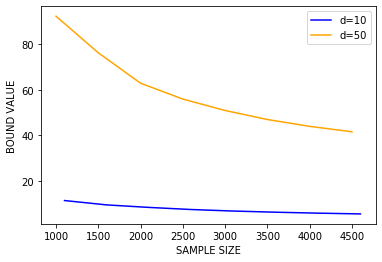
Figure 1: Evaluation of the right hand side in Thm. 6.1 with $d=10$ and $d=50$.

Discussion.

To the the best of our knowledge, this is the first attempt to numerically compute PAC-Bayes bounds for unbounded problems, making it impossible to compare to other results. We stress though that obtaining numerical values for the bound without assuming a bounded loss is a significant first step. Furthermore, we consider a rather hard problem: $f$ is not linear, so we cannot rely on a linear approximation fitting perfectly data, and the larger the dimension, the larger the error, as illustrated by Fig. 1. Thus for any posterior $Q$, the quantity $\mathbb{E}_{h\sim Q}[R(h)]$ is potentially large in practice and our bound might not be tight. Finally, notice that optimising $\alpha$ (instead of taking $\alpha=1/2$ to recover a classic convergence rate) leads to a significantly better bound. A numerical example of this assertion is presented in Appendix A. We aim to conduct further studies to consider the convergence rate as an hyperparameter to optimise, rather than selecting the same rate for all terms in the bound.

8 Conclusion

The main goal of this paper is to expand the PAC-Bayesian theory to learning problems with unbounded losses, under the HYPE condition. We plan next to particularise our general theorems to more specific situations, starting with the kernel PCA setting.

Appendix A Additional experiments for the bounded loss case

Our experimental framework has been inspired of the work of Mhammedi et al. (2019).
Settings We generate synthetic data for classification, and we are using the 0-1 loss. Here, the data space is $\mathcal{Z}=\mathcal{X}\times\mathcal{Y}=\mathbb{R}^{d}\times\{0,1\}$ with $d\in\mathbb{N}$. Here the set of predictors $\mathcal{H}$ is also $\mathbb{R}^{d}$. And for $z=(x,y)\in\mathcal{Z},h\in\mathcal{H}$, we define the loss as $\ell(h,z):=|\mathds{1}\left\{\phi(h^{\top}x)>1/2\right\}-y|$. where $\phi(w)=\frac{1}{1+e^{-w}}$ We want to learn an optimised predictor given a dataset $\mathcal{S}=(z_{i}=(x_{i},y_{i}))_{i=1..m}$. To do so we use regularised logistic regression and we compute:

$$\hat{h}(\mathcal{S}):=\text{arg}\min_{h\in\mathcal{H}}\lambda\frac{||h||^{2}}{2}-\frac{1}{m}\sum_{i=1}^{m}y_{i}\log\left(\phi(h^{\top}x_{i})\right)+(1-y_{i})\log\left(1-\phi(h^{\top}x_{i})\right)$$ (2)

where $\lambda$ is a fixed regularisation parameter. We also define

$$\mathcal{M}_{1}^{+}(\mathcal{H}):=\left\{\mathcal{N}(h,\sigma^{2}I_{d})\mid h\in\mathcal{H},\sigma^{2}\in\mathbb{R}^{+}\right\}$$

which is the set of considered measures for this learning problem.
Parameters We set $\delta=0.05,\lambda=0.01$. We approximately solve Eq. 2 by using the minimize function of the optimisation module in Python, with the Powell method. To approximate gaussian expectations, we use Monte-Carlo sampling.
Synthetic data We generate synthetic data for $d=10$ according to the following process: for a fixed sample size $m$, we draw $x_{1},...,x_{m}$ under the multivariate gaussian distribution $\mathcal{N}(0,I_{d})$ and we compute for all $i$: $y_{i}=\mathds{1}\{\phi(h^{*\top}x_{i})>1/2\}$ where $h^{*}$ is the vector formed by the $d$ first digits of $\pi$.
Normalisation trick Given the predictors shape, we notice that for any $h\in\mathcal{H}$:

$$\mathds{1}\{\phi(h^{*\top}x)>1/2\}=1\Leftrightarrow\frac{1}{1+\exp(-h^{\top}x)}>\frac{1}{2}\Leftrightarrow h^{\top}x<0$$

Thus, the value of the prediction is exclusively determined by the sign of the inner product, and this quantity is definitely not influenced by the norm of the vector.
Then, for any sample $\mathcal{S}$, we call normalisation trick the fact of considering $\hat{h}(\mathcal{S})/||\hat{h}(\mathcal{S})||$ instead of $\hat{h}(\mathcal{S})$ in our calculations. This process will not deteriorate the quality of the prediction and will considerably enhance the value of the KL divergence.
First experiment Our goal here is to highlight the point discussed in Remark 4.3 e.g. the influence of the parameter $\alpha$ in Proposition 4.1. We fix arbitrarily $\sigma_{0}^{2}=1/2$ and we define our naive prior as $P_{0}=\mathcal{N}(0,\sigma_{0}^{2}I_{d})$. For a fixed dataset $\mathcal{S}$, we define our posterior as $P(\mathcal{S}):=\mathcal{N}(\hat{h}(\mathcal{S}),\sigma^{2}I_{d})$, with $\sigma^{2}\in\{1/2,...,1/2^{J}\},(J=\log_{2}(m))$ such that it is minimising the bound among candidates.
We computed two curves: first, Proposition 4.1 with $\alpha=1/2$ second, Proposition 4.1 again with $\alpha$ equals to the value proposed in Lemma 4.4. Notice that to compute this last bound, we first optimised our choice of posterior with $\alpha=1/2$ and we then optimised $\alpha$. We did this to be consistent with Lemma 4.4. Indeed, we proved this lemma by assuming that the KL divergence was already fixed, hence our optimisation process in two steps. We chose to apply the normalisation trick here, we then obtained the left curve of Fig. 2.

Discussion From this curve, we formulate several remarks. First, we remark on this specifc case, our theorem provide a quite tight result in practice ( with an error rate lesser than $10\%$ for the bound with optimised alpha).
Secondly we can now confirm that choosing an optimised $\alpha$ leads to a tighter bound: in further studies, it will relevant to adjust $\alpha$ with regards to the different terms of our bound instead of looking for an identical convergence rate for all the terms.

Second experiment We want now to study Proposition 4.6 e.g. to see if an informed prior provide effectively a tighter bound than a naive one. We will use the notations introduced in Proposition 4.6. For a dataset $\mathcal{S}$ we define $h_{1}(\mathcal{S})=h(\mathcal{S}_{>m/2})$ the vector resulting of the optimisation of Eq. 2 on $\mathcal{S}_{>m/2}$. We define similarly $h_{2}(\mathcal{S}):=h(\mathcal{S}_{\leq m/2})$. We fix arbitrarily $\sigma_{0}^{2}=1/2$ and we define our informed priors as $P_{1}=\mathcal{N}(h_{1}(\mathcal{S}),\sigma_{0}^{2}I_{d})$ and $P_{2}=\mathcal{N}(h_{2}(\mathcal{S}),\sigma_{0}^{2}I_{d})$. Finally, we define our posterior as $P(\mathcal{S}):=\mathcal{N}(\hat{h}(\mathcal{S}),\sigma^{2}I_{d})$, with $\sigma^{2}\in\{1/2,...,1/2^{J}\},(J=\log_{2}(m))$ with $\sigma^{2}$ optimising the bound among the same candidate than the first experiment.
We computed two curves: first, Proposition 4.1 with $\alpha$ optimised accordingly to Lemma 4.4 secondly, Proposition 4.6 with $\alpha_{1},\alpha_{2}$ optimised as well and the informed priors as defined above. We chose to not apply the normalisation trick here, we then obtained the right curve of Fig. 2:

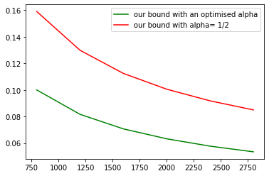
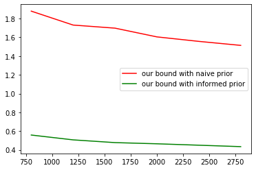
Figure 2: On the left, result of the first experiment which highlight the importance of optimising $\alpha$. On the right, result of the second experiment which show how effective an informed prior is.

Discussion

We clearly see that with this framework having an informed prior is a powerful tool to enhance the quality of our bound. Notice that we voluntarily chose to not apply the normalisation trick here. The reason behind this is that this trick appears to be too powerful in practice, and applying it leads to be counterproductive to highlight our point: the bound without informed prior would be tighter than the one with. Furthermore, this trick is very linked to the specific structure of our problem and is not valid for any classification problem. Thus, the idea of providing informed priors remains an interesting tool for most of the cases.

Appendix B Existing work

B.1 Germain et al., 2016

In Germain et al. (2016, Section 4), a PAC-Bayesian bound has been provided for all sub-gamma losses with a variance $s^{2}$ and scale parameter $c$, under a data distribution $\mu$ and a prior $P$, i.e. losses satisfying the following property:

$$\forall\lambda\in(0,\frac{1}{c}),\log\left(\frac{1}{\delta}\mathbb{E}_{h\sim P}\mathbb{E}_{\mathcal{S}}\;e^{\lambda(R(h)-R_{m}(h))}\right)\leq\frac{s^{2}}{c^{2}}(-\log(1-c\lambda)-\lambda c)\leq\frac{\lambda^{2}s^{2}}{2(1-c\lambda)}.$$

Note that a sub-gamma loss (with regards to $\mu$ and $P$) is potentially unbounded. Germain et al. then propose the following PAC-Bayesian bound:

Theorem B.1 (Germain et al., 2016).

If the loss $\ell$ is sub-gamma with a variance $s^{2}$ and scale parameter $c$, under the data distribution $\mu$ and a fixed prior $P\in\mathcal{H}$, then we have, with probability $1-\delta$ over size-$m$ samples, for any $Q\ll P$:

$$\mathbb{E}_{h\sim Q}\left[R(h)\right]\leq\mathbb{E}_{h\sim Q}\left[R_{m}(h)\right]+\frac{\operatorname{KL}(Q||P)+\log(1/\delta)}{m}+\frac{s^{2}}{2(1-c)}$$

Thm. B.1 will be quoted several times in this paper given that it is a concrete PAC Bayesian bound provided with the will to overcome the constraint of a bounded loss. It is also one of the only one found in literature by the authors.

Can we apply this theorem to the bounded case?

The answer is yes: we remark that thanks to Hoeffding’s lemma, if $\ell$ is bounded by $C$, then for any $h\in\mathcal{H}$, $R_{m}(h)-R(h)\in[-C,C]$ almost surely. So, $\forall\lambda\in\mathbb{R},$ $\log\mathbb{E}_{z\sim\mu}\left[e^{\lambda(R(h)-R_{m}(h)}\right]\leq\frac{\lambda^{2}C^{2}}{2}$. So, for any prior $P$, $\log\mathbb{E}_{h\sim P}\mathbb{E}_{z\sim\mu}\left[e^{\lambda(R(h)-R_{m}(h)}\right]\leq\frac{\lambda^{2}C^{2}}{2}$.
Thus, $\ell$ is sub-gamma with variance $C^{2}$ and scale parameter 0. So Thm. B.1 can be applied with $s^{2}=C^{2}$, $c=0$.

Comparison with Proposition 4.1

We remark that by taking $K=C$ and $\alpha=1$ in Proposition 4.1, we are recovering Thm. B.1. However, our approach allows us to say that if we can obtain a more precise form of $K$ such that $\forall h\in\mathcal{H}$, $K(h)\leq C$ and $K$ is non-constant, Thm. 3.4, will ensure us that

$$\frac{1}{m^{\alpha}}\log\left(\mathbb{E}_{h\sim P}\left[\exp\left(\frac{K(h)^{2}}{2m^{1-2\alpha}}\right)\right]\right)\leq\frac{C^{2}}{2m^{1-\alpha}}$$

Thus, having a precise information on the behavior of the loss function $\ell$ with regards to the predictor $h$ allows us to obtain a tighter control of the exponential moment, hence a tighter bound.

Remark B.2.

We can see that Thm. B.1, one can’t control the factor $C^{2}/2$. However, the authors remarked this apparent weakness and partially corrected this issue on (Germain et al., 2016, Section 4, Eq (13),(14)). Indeed, they proposed to balance the influence of $m$ between the different terms of the PAC Bayesian bound by providing to all terms the same convergence rate in $1/\sqrt{m}$.

We then can see Proposition 4.1 as a proper generalisation of (Germain et al., 2016, Section 4, Eq (13),(14)). Indeed, our bound exhibits properly the influence of the parameter $\alpha$. Thus, we understand (and Lemma 4.4 proves it) that the choice of $\alpha$ deserves a study in itself in the way it is now a parameter of our optimisation problem. This fact has already be higlightened in Alquier et al. (2016, Theorem 4.1) (where $\lambda:=m^{\alpha}$).

B.2 Holland, 2019

Holland (2019) proposed a PAC Bayesian inequality with unbounded loss. For that he introduced a function $\psi$ verifying a few specific conditions, different of those we used in Sec. 5 to define our set of softening functions. Indeed he considered a function $\psi$ such that:

• $\psi$ is bounded,

• $\psi$ is non decreasing,

• it exists $b>0$ such that for all $u\in\mathbb{R}$:

  $$-\log\left(1-u+\frac{u^{2}}{b}\right)\leq\psi(u)\leq\log\left(1+u+\frac{u^{2}}{b}\right).$$ (3)

We remark that, as Holland did, we supposed that our softening functions are non-decreasing. We chose softening functions to be equal to $Id$ on $[0,1]$ which is quite restrictive but we are just imposing softening functions to be lesser than $Id$ on $\left[1,+\infty\right)$ where Holland supposed $\psi$ to be bounded and satisfy Eq. 3. A concrete example of such a function $\psi$ lies in the piecewise polynomial function of Catoni and Giulini (2017), defined by:

$$\psi(u)=\begin{cases}-2\sqrt{2}/3&\text{ if }u\leq-\sqrt{2}\\ u-u^{3}/6&\text{ if }u\in[-2\sqrt{2}/3,2\sqrt{2}/3]\\ 2\sqrt{2}/3&\text{otherwise.}\end{cases}$$

As in Sec. 5, we are considering the $\psi$-empirical risk $R_{m},\psi,s$ for any $s>0$. Holland provided his theorem given the fact the following assumptions are realised:

• Bounds on lower-order moments. For all $h\in\mathcal{H}$, we have $\mathbb{E}_{z\sim\mu}[\ell(h,z)^{2}]\leq M_{2}<+\infty$, $\mathbb{E}_{z\sim\mu}[\ell(h,z)^{3}]\leq M_{3}<+\infty$.

• Bounds on the risk. For all $h\in\mathcal{H}$, we suppose $R(h)\leq\sqrt{mM_{2}/(4\log(\delta^{-1})}$.

• Large enough confidence, we require $\delta\leq e^{-1/9}$.

Now we can state Holland’s theorem.

Theorem B.3 (Holland, 2019).

Let $P$ be a prior distribution on model $\mathcal{H}$. Let the three assumptions listed above hold. Setting $s^{2}=mM_{2}/(2\log(\delta^{-1}))$, then with probability at least $1-\delta$ over the random draw of the size-$m$ sample, it holds that

$$\mathbb{E}_{h\sim Q}\left[R(h)\right] \leq\mathbb{E}_{h\sim Q}\left[R_{m,\psi,s}(h)\right]+\frac{1}{\sqrt{m}}\left(\operatorname{KL}(Q||P)+\frac{1}{2}\log\left(\frac{8\pi M_{2}}{\delta^{2}}\right)-1\right)$$

$$+\frac{1}{\sqrt{m}}\nu^{*}(\mathcal{H})+O\left(\frac{1}{m}\right)$$

where $\nu^{*}(\mathcal{H}):=\mathbb{E}_{h\sim P}\left[\exp\left(\sqrt{m}(R(h)-R_{m,\psi,s}(h))\right)\right]\hskip 2.84526pt/\hskip 2.84526pt\mathbb{E}_{h\sim P}\left[\exp\left(R(h)-R_{m,\psi,s}(h)\right)\right]$

Appendix C Exponential moment via tail integrals

This section provides a bound of the exponential moment when $D(x,y)=(x-y)^{2}$ by only using classic properties, i.e. without the self-bounding property.

Theorem C.1.

Let $h$ be a fixed predictor, $\alpha\in\mathbb{R}$ and $\mathcal{S}=(z_{1},...,z_{m})$ be the $m$-sample of data. If the loss $\ell$ satisfies the HYPE condition with $K(h)$, then we have:

$$\mathbb{E}_{\mathcal{S}}\left[e^{m^{\alpha}\Delta(h)^{2}}\right]\leq 1+\frac{2}{1-\frac{m^{1-\alpha}}{2K(h)^{2}}}\left[\exp\left(m^{\alpha}K(h)^{2}-\frac{m}{2}\right)-1\right].$$

Recall that $\Delta(h):=R(h)-R_{m}(h)$.

Proof.First let us notice that almost surely we have:

$$\forall i,\hskip 8.53581pt0\leq\ell(h,z_{i})\leq K(h),\;\text{ so }\Delta(h)\leq K(h).$$ (4)

Then

$$\mathbb{E}_{\mathcal{S}}\left[e^{m^{\alpha}\Delta(h)^{2}}\right] =\int_{0}^{+\infty}\mathbb{P}\left(e^{m^{\alpha}\Delta(h)^{2}}>t\right)dt$$

$$\leq 1+\int_{1}^{+\infty}\mathbb{P}\left(\exp\left(m^{\alpha}\Delta(h)^{2}\right)>t\right)dt$$

$$\leq 1+\int_{0}^{+\infty}\mathbb{P}\left(\exp\left(m^{\alpha}\Delta(h)^{2}\right)>e^{u^{2}}\right)2ue^{u^{2}}du (t=e^{u^{2}})$$

$$\leq 1+\int_{0}^{\sqrt{m}^{\alpha}K(h)}\mathbb{P}\left(\exp\left(m^{\alpha}\Delta(h)^{2}\right)>e^{u^{2}}\right)2ue^{u^{2}}du$$ (thanks to Eq. 4)

$$\leq 1+\int_{0}^{\sqrt{m}^{\alpha}K(h)}\mathbb{P}\left(|\Delta(h)|>m^{\frac{\alpha}{2}}u\right)2ue^{u^{2}}du.$$

Thanks to Eq. 4, we can use Hoeffding’s inequality on $R_{m}(h)$. We thus obtain:

$$\forall u>0,\hskip 8.53581pt\mathbb{P}\left(|\Delta(h)|>m^{\frac{\alpha}{2}}u\right) \leq 2\exp\left(-\frac{u^{2}}{2m^{\alpha}\sum_{i=1}^{m}(\frac{K(h)}{m})^{2}}\right)$$

$$\leq 2\exp\left(-\frac{m^{1-\alpha}u^{2}}{2K(h)^{2}}\right).$$

So by application of this inequality and the change of variable $v=u^{2}$ we have:

$$\mathbb{E}_{\mathcal{S}}\left[e^{m^{\alpha}\Delta(h)^{2}}\right] \leq 1+\int_{0}^{m^{\alpha}K(h)^{2}}2\exp\left(v-\frac{vm^{1-\alpha}}{2K(h)^{2}}\right)dv$$

$$\leq 1+\frac{2}{1-\frac{m^{1-\alpha}}{2K(h)^{2}}}\left[\exp\left(m^{\alpha}K(h)^{2}-\frac{m}{2}\right)-1\right]$$

which completes the proof. ∎

Appendix D A corollary of Theorem 5.5

We are now dealing with the following assumption on $K$: it exists a constant $M_{3}$ such that:

$$\sup_{Q\in\mathcal{M}_{1}^{+}(\mathcal{H})}\hskip 5.69054pt\mathbb{E}_{h\sim Q}[K(h)^{3}]\leq M_{3}<+\infty.$$ (5)

In other words, we assume that the third moments under any posterior distribution are uniformly bounded by a fixed constant $M_{3}$. Thus, this is a stronger assumption than Eq. 1.
Under this assumption, we can properly define the (finite) following quantity:

$$\forall s>0,\hskip 2.84526ptM_{3,s}:=\sup_{Q\in\mathcal{M}_{1}^{+}(\mathcal{H})}\mathbb{E}_{h\sim Q}\left[K(h)^{3}\mathds{1}\left\{K(h)\geq s\right\}\right]\leq M_{3}.$$

Lemma D.1.

Assume that Eq. 5 holds and let $\psi\in\mathcal{F}$, $Q\in\mathcal{M}_{1}^{+}(\mathcal{H}),s>0$. We have :

$$\mathbb{E}_{h\sim Q}[R(h)]\leq\mathbb{E}_{h\sim Q}[R_{\psi,s}(h)]+\frac{M_{3,s}}{s^{2}}.$$

Proof.The beginning of the proof of Lemma 5.4 holds here. We then have for any $h\in\mathcal{H}$:

$$R(h)-R_{\psi,s}(h)\leq K(h)\mathbb{P}_{z\sim\mu}\left\{\ell(h,z)\geq s\right\}\mathds{1}\left\{K(h)\geq s\right\}.$$

Yet, by Markov’s inequality, we have:

$$\mathbb{P}_{z\sim\mu}\left\{\ell(h,z)\geq s\right\} \leq\frac{\mathbb{E}_{z\sim\mu}\left[\ell(h,z)^{2}\right]}{s^{2}}\leq\frac{K(h)^{2}}{s^{2}}.$$

So we can finally affirm that:

$$R(h)\leq R_{\psi,s}(h)+\frac{K(h)^{3}}{s^{2}}\mathds{1}\left\{K(h)\geq s\right\}.$$

Hence the result by integrating over $\mathcal{H}$ with $Q$ and bounding $\mathbb{E}_{h\sim Q}[K(h)^{3}\mathds{1}\left\{K(h)\geq s\right\}]$ by $M_{3,s}$. ∎

Finally we present the following theorem, which is a corollary of Thm. 5.5:

Theorem D.2.

Let $\ell$ being $\texttt{HYPE}(K)$ compliant and assume that $K$ is satisfying Eq. 5. Then for any prior $P\in\mathcal{M}_{1}^{+}(\mathcal{H})$ with no data dependency, for any $\alpha\in\mathbb{R}$, for any $\psi\in\mathcal{F}$ and for any $\delta\in[0:1]$, we have with probability at least $1-\delta$ over size-$m$ samples $\mathcal{S}$, for any $Q$ such that $Q\ll P$ and $P\ll Q$:

$$\mathbb{E}_{h\sim Q}\left[R(h)\right] \leq\mathbb{E}_{h\sim Q}\left[R_{m,\psi,s}(h)\right]+\frac{M_{3,s}}{s^{2}}+\frac{\operatorname{KL}(Q||P)+\log\left(\frac{1}{\delta}\right)}{m^{\alpha}}$$

$$+\frac{1}{m^{\alpha}}\log\left(\mathbb{E}_{h\sim P}\left[\exp\left(\frac{s^{2}}{2m^{1-2\alpha}}\psi\left(\frac{K(h)}{s}\right)^{2}\right)\right]\right).$$

Proof.The proof is similar to that of Thm. 5.5, we simply use Lemma D.1 instead of Lemma 5.4. ∎

Remark D.3.

A possible choice for the pair $(\alpha,s)$ is $s^{2}=\sqrt{m},\alpha=1/2$. In this way we recover the same convergence rate in $1/\sqrt{m}$ than Holland (2019) for all the terms on the right-hand side of the bound. Furthermore, with those parameters we recover in the exponential moment the factor $\sqrt{m}$ also visible in $\nu^{*}(\mathcal{H})$ (cf Thm. B.3).

Appendix E Proofs

E.1 Proof of Theorem 2.2

Proof.Let $D:\mathbb{R}^{+}\times\mathbb{R}^{+}\mapsto\mathbb{R}$ a convex function, $\alpha\in\mathbb{R},P$ a fixed prior and $\delta\in[0,1]$. Since $\mathbb{E}_{h\sim P}\left[e^{m^{\alpha}D(R_{m}(h),R(h))}\right]$ is a nonnegative random variable, we know that, by Markov’s inequality, for any $h\in\mathcal{H}$ :

$$\mathbb{P}\left(\mathbb{E}_{h\sim P}\left[e^{m^{\alpha}D(R_{m}(h),R(h))}\right]>\frac{1}{\delta}\mathbb{E}_{\mathcal{S}}\hskip 2.84526pt\mathbb{E}_{h\sim P}\left[e^{m^{\alpha}D(R_{m}(h),R(h))}\right]\right)\leq\delta.$$

So with probability $1-\delta$, we have:

$$\mathbb{E}_{h\sim P}\left[e^{m^{\alpha}D(R_{m}(h),R(h))}\right]\leq\frac{1}{\delta}\mathbb{E}_{\mathcal{S}}\hskip 2.84526pt\mathbb{E}_{h\sim P}\left[e^{m^{\alpha}D(R_{m}(h),R(h))}\right].$$

We will now apply the logarithm function on each side of this inequality. Furthermore, because of the positiveness of $e^{m^{\alpha}D(R_{m}(h),R(h))}$ and because we supposed the prior $P$ to have no data dependency, we can switch the expectation symbols by Fubini-Tonelli’s theorem: so with probability $1-\delta$ over samples $\mathcal{S}$, we have:

$$\log\left(\mathbb{E}_{h\sim P}\left[e^{m^{\alpha}D(R_{m}(h),R(h))}\right]\right)\leq\log\left(\frac{1}{\delta}\mathbb{E}_{h\sim P}\hskip 2.84526pt\mathbb{E}_{\mathcal{S}}\left[e^{m^{\alpha}D(R_{m}(h),R(h))}\right]\right).$$

We now rename $A:=\log\left(\mathbb{E}_{h\sim P}\left[e^{m^{\alpha}D(R_{m}(h),R(h))}\right]\right)$.

Furthermore, if we denote by $\frac{dQ}{dP}$ the Radon-Nikodym derivative of $Q$ with respect to $P$ when $Q\ll P$, we then have, for all $Q$ such that $Q\ll P$ and $P\ll Q$:

$$A =\log\left(\mathbb{E}_{h\sim Q}\left[\frac{dP}{dQ}e^{m^{\alpha}D(R_{m}(h),R(h))}\right]\right)$$

$$=\log\left(\mathbb{E}_{h\sim Q}\left[\left(\frac{dQ}{dP}\right)^{-1}e^{m^{\alpha}D(R_{m}(h),R(h))}\right]\right) \frac{dP}{dQ}=\left(\frac{dQ}{dP}\right)^{-1}$$

$$\geq-\mathbb{E}_{h\sim Q}\left[\log\left(\frac{dQ}{dP}\right)\right]+\mathbb{E}_{h\sim Q}\left[m^{\alpha}D(R_{m}(h),R(h))\right]$$ (by concavity of log with Jensen’s inequality)

$$\geq-\operatorname{KL}(Q||P)+m^{\alpha}\mathbb{E}_{h\sim Q}\left[D(R_{m}(h),R(h))\right]$$

$$\geq-\operatorname{KL}(Q||P)+m^{\alpha}D\left(\mathbb{E}_{h\sim Q}\left[\left(R_{m}(h),R(h)\right)\right]\right) D$$ (by convexity of with Jensen’s inequality)

$$\geq-\operatorname{KL}(Q||P)+m^{\alpha}D\left(\mathbb{E}_{h\sim Q}\left[R_{m}(h)\right],\mathbb{E}_{h\sim Q}\left[R(h)\right]\right).$$

Hence, for $Q$ such that $Q\ll P$ and $P\ll Q$,

$$D\left(\mathbb{E}_{h\sim Q}\left[R_{m}(h)\right],\mathbb{E}_{h\sim Q}\left[R(h)\right]\right) \leq\frac{1}{m^{\alpha}}\left(\operatorname{KL}(Q||P)+A\right).$$

So with probability $1-\delta$, for $Q$ such that $Q\ll P$ and $P\ll Q$,

$$D\left(\mathbb{E}_{h\sim Q}\left[R_{m}(h)\right],\mathbb{E}_{h\sim Q}\left[R(h)\right]\right) \leq\frac{1}{m^{\alpha}}\left(\operatorname{KL}(Q||P)+\log\left(\frac{1}{\delta}\mathbb{E}_{h\sim P}\mathbb{E}_{\mathcal{S}}\;e^{m^{\alpha}D(R_{m}(h),R(h))}\right)\right).$$

This completes the proof of Theorem 2.2. ∎

E.2 Proof of Theorem 6.1

We first provide a technical property. Recall that

$$\xi=\mathbb{E}_{h\sim P}\left[\exp\left(\frac{K(h)^{2}}{2m^{1-2\alpha}}\right)\right].$$

Proposition E.1.

Let $\alpha\in\mathbb{R}$. If the loss $\ell$ is $\texttt{HYPE}(K)$ compliant with $K(h)=B||h||+C$, with $B>0$, $C\geq 0$, then we have, for any Gaussian prior $P=\mathcal{N}(0,\sigma^{2}\textbf{I}_{N})$ with $\sigma^{2}=t\frac{m^{1-2\alpha}}{B^{2}}$,  $0<t<1$ and $N\geq 6$:

$$\xi\leq 2\exp\left(\frac{C^{2}}{2m^{1-2\alpha}f(t)}\left(1+f(t)\right)\right)\frac{1}{\left(\sqrt{1-t}\right)^{N}}\left(1+\left(\frac{C}{\sqrt{2f(t)m^{1-2\alpha}}}\right)\right)^{N-1}$$

with $f(t)=\frac{1-t}{t}$.

Proof. We recall that $\sigma^{2}=t\frac{m^{1-2\alpha}}{B^{2}}$. By expliciting the expectation and $K(h)$ we thus obtain:

$$\xi =\left(\frac{1}{\sqrt{2\pi\sigma^{2}}}\right)^{N}\int_{h\in\mathbb{R}^{N}}\exp\left(\frac{(B||h||+C)^{2}}{2m^{1-2\alpha}}-\frac{||h||^{2}B^{2}}{2tm^{1-2\alpha}}\right)dh$$

$$=\left(\frac{1}{\sqrt{2\pi\sigma^{2}}}\right)^{N}\int_{h\in\mathbb{R}^{N}}\exp\left(-\frac{1}{2m^{1-2\alpha}}\left(f(t)B^{2}||h||^{2}-2BC||h||-C^{2}\right)\right)dh$$

$$=\left(\frac{1}{\sqrt{2\pi\sigma^{2}}}\right)^{N}\int_{h\in\mathbb{R}^{N}}\exp\left(-\frac{B^{2}f(t)}{2m^{1-2\alpha}}\left(||h||^{2}-\frac{2C||h||}{Bf(t)}-\frac{C^{2}}{B^{2}f(t)}\right)\right)dh$$

$$=\exp\left(\frac{C^{2}}{2m^{1-2\alpha}f(t)}\left(1+f(t)\right)\right)\frac{1}{(\sqrt{2\pi\sigma^{2}})^{N}}\int_{h\in\mathbb{R}^{N}}\exp\left(-\frac{B^{2}f(t)}{2m^{1-2\alpha}}\left(||h||-\frac{C}{Bf(t)}\right)^{2}\right)dh.$$

We will use the spherical coordinates in $N$-dimensional Euclidean space given in Blumenson (1960):

$$\varphi:(h_{1},...,h_{N})\rightarrow(r,\varphi_{1},...,\varphi_{N-1})$$

where especially $r=||h||$ and also the Jacobian of $\phi$ is given by:

$$d^{N}V=r^{N-1}\prod_{k=1}^{N-2}\sin^{k}(\varphi_{N-1-k})=r^{N-1}d_{S^{N-1}}V.$$

Let us also precise that as given in Blumenson (1960, page 66), we have that the surface of the sphere of radius 1 in $N$-dimensional space is:

$$\int_{\varphi_{1},...,\varphi_{N-1}}d_{S^{N-1}}V\hskip 2.84526ptd{\varphi_{1}}...d{\varphi_{N-1}}=\frac{2\sqrt{\pi}^{N}}{\Gamma\left(\frac{N}{2}\right)}$$

where $\Gamma$ is the Gamma function defined as:

$$\Gamma(x)=\int_{0}^{+\infty}t^{x-1}e^{-t}dt\hskip 14.22636pt\text{for}\hskip 5.69054ptx>-1.$$

Then, if we set

$$A:=\int_{h\in\mathbb{R}^{N}}\exp\left(-\frac{B^{2}f(t)}{2m^{1-2\alpha}}\left(||h||-\frac{C}{Bf(t)}\right)^{2}\right)dh$$

we obtain by a change of variable:

$$A =\int_{r,\varphi_{1},...,\varphi_{N-1}}\exp\left(-\frac{B^{2}f(t)}{2m^{1-2\alpha}}\left(r-\frac{C}{Bf(t)}\right)^{2}\right)d^{N}V\hskip 2.84526ptdrd{\varphi_{1}}...d{\varphi_{N-1}}$$

$$=\left(\frac{2\sqrt{\pi}^{N}}{\Gamma\left(\frac{N}{2}\right)}\right)\int_{r=0}^{+\infty}\exp\left(-\frac{B^{2}f(t)}{2m^{1-2\alpha}}\left(r-\frac{C}{Bf(t)}\right)^{2}\right)r^{N-1}dr$$

$$=\left(\frac{2\sqrt{\pi}^{N}}{\Gamma\left(\frac{N}{2}\right)}\right)\int_{r=-\frac{C}{Bf(t)}}^{+\infty}\left(r+\frac{C}{Bf(t)}\right)^{N-1}\exp\left(-\frac{B^{2}f(t)}{2m^{1-2\alpha}}r^{2}\right)dr$$

$$=\left(\frac{2\sqrt{\pi}^{N}}{\Gamma\left(\frac{N}{2}\right)}\right)\sum_{k=0}^{N-1}\binom{N-1}{k}\left(\frac{C}{Bf(t)}\right)^{N-k-1}\int_{r=-\frac{C}{Bf(t)}}^{+\infty}r^{k}\exp\left(-\frac{B^{2}f(t)}{2m^{1-2\alpha}}r^{2}\right)dr.$$

We fix a random variable $X$ such that

$$X\sim\mathcal{N}\left(0,\frac{m^{1-2\alpha}}{B^{2}(f(t)}\right).$$

We then have for any $k$ positive integer, if $k$ is even:

$$\int_{r=-\frac{C}{Bf(t)}}^{+\infty}r^{k}\exp\left(-\frac{B^{2}f(t)}{2m^{1-2\alpha}}r^{2}\right)dr \leq\int_{r=-\infty}^{+\infty}r^{k}\exp\left(-\frac{B^{2}f(t)}{2m^{1-2\alpha}}r^{2}\right)dr$$

$$\leq\sqrt{2\pi\frac{m^{1-2\alpha}}{B^{2}f(t)}}\mathbb{E}[|X|^{k}].$$

And if $k$ is odd:

$$\int_{r=-\frac{C}{Bf(t)}}^{+\infty}r^{k}\exp\left(-\frac{B^{2}f(t)}{2m^{1-2\alpha}}r^{2}\right)dr \leq\int_{r=0}^{+\infty}r^{k}\exp\left(-\frac{B^{2}f(t)}{2m^{1-2\alpha}}r^{2}\right)dr$$

$$\leq\sqrt{2\pi\frac{m^{1-2\alpha}}{B^{2}f(t)}}\mathbb{E}[|X|^{k}\mathds{1}(X\geq 0)]$$

$$\leq\sqrt{2\pi\frac{m^{1-2\alpha}}{B^{2}f(t)}}\mathbb{E}[|X|^{k}].$$

So we have:

$$A \leq\left(\frac{2\sqrt{\pi}^{N}}{\Gamma\left(\frac{N}{2}\right)}\right)\sum_{k=0}^{N-1}\binom{N-1}{k}\left(\frac{C}{Bf(t)}\right)^{N-k-1}\sqrt{2\pi\frac{m^{1-2\alpha}}{B^{2}f(t)}}\mathbb{E}[|X|^{k}].$$

As precised in Winkelbauer (2012), we have for any $k$:

$$\mathbb{E}[|X|^{k}]=\left(\sqrt{\frac{m^{1-2\alpha}}{B^{2}f(t)}}\right)^{k}2^{k/2}\frac{\Gamma\left(\frac{k+1}{2}\right)}{\sqrt{\pi}}.$$

So finally:

$$A \leq 2\sqrt{\pi}^{N}\hskip 2.84526pt\sum_{k=0}^{N-1}\binom{N-1}{k}\left(\frac{C}{Bf(t)}\right)^{N-k-1}\left(\sqrt{\frac{2m^{1-2\alpha}}{B^{2}f(t)}}\right)^{k+1}\frac{\Gamma\left(\frac{k+1}{2}\right)}{\Gamma\left(\frac{N}{2}\right)}.$$

Lemma E.2.

If $N\geq 6$, then:

$$\max_{k=0..N-1}\frac{\Gamma\left(\frac{k+1}{2}\right)}{\Gamma\left(\frac{N}{2}\right)}=1.$$

Proof.As precised in the introduction of Srinivasan and Zvengrowski (2011), Gauss (2011, page 147) proved that on the interval $[x_{0},+\infty)$ where $x_{0}\in[1.46,1.47]$, $\Gamma$ is a monotonic increasing function. So, for $N-1\geq k\geq 2,\Gamma(\frac{k+1}{2})\leq\Gamma(\frac{N}{2})$. And because $\Gamma(1/2)=\sqrt{\pi},\Gamma(1)=1$, we have

$$\max_{k=0..N-1}\frac{\Gamma\left(\frac{k+1}{2}\right)}{\Gamma\left(\frac{N}{2}\right)}=\max\left(\frac{\sqrt{\pi}}{\Gamma\left(\frac{N}{2}\right)},\frac{\Gamma\left(\frac{N-1+1}{2}\right)}{\Gamma\left(\frac{N}{2}\right)}\right)=\max\left(\frac{\sqrt{\pi}}{\Gamma\left(\frac{N}{2}\right)},1\right)$$

And because $N\geq 6$ and that $\Gamma$ is monotone increasing on $[3;+\infty]$, we have $\Gamma(N/2)\geq\Gamma(3)\geq\sqrt{\pi}$. Hence the result. ∎
Using Lemma E.2 allows us to write:

$$A \leq 2\sqrt{\pi}^{N}\hskip 2.84526pt\sum_{k=0}^{N-1}\binom{N-1}{k}\left(\frac{C}{Bf(t)}\right)^{N-k-1}\left(\sqrt{\frac{2m^{1-2\alpha}}{B^{2}f(t)}}\right)^{k+1}.$$

We recall that $\sigma^{2}=t\frac{m^{1-2\alpha}}{B^{2}}$ and $f(t)=\frac{1-t}{t}$. Then we can write:

$$A\leq 2\sqrt{\pi}^{N}\hskip 2.84526pt\sum_{k=0}^{N-1}\binom{N-1}{k}\left(\frac{C}{Bf(t)}\right)^{N-k-1}\left(\sqrt{\frac{2\sigma^{2}}{1-t}}\right)^{k+1}.$$

We now conclude with the final bound on $\xi$

$$\xi \leq\exp\left(\frac{C^{2}}{2m^{1-2\alpha}f(t)}\left(1+f(t)\right)\right)\frac{1}{(\sqrt{2\pi\sigma^{2}})^{N}}\hskip 2.84526ptA$$

$$\leq\exp\left(\frac{C^{2}}{2m^{1-2\alpha}f(t)}\left(1+f(t)\right)\right)\frac{1}{(\sqrt{2\pi\sigma^{2}})^{N}}2\sqrt{\pi}^{N}\hskip 2.84526pt\sum_{k=0}^{N-1}\binom{N-1}{k}\left(\frac{C}{Bf(t)}\right)^{N-k-1}\left(\sqrt{\frac{2\sigma^{2}}{1-t}}\right)^{k+1}$$

$$\leq 2\exp\left(\frac{C^{2}}{2m^{1-2\alpha}f(t)}\left(1+f(t)\right)\right)\sum_{k=0}^{N-1}\binom{N-1}{k}\left(\frac{C}{Bf(t)}\right)^{N-k-1}\left(\sqrt{\frac{1}{1-t}}\right)^{k+1}\left(\sqrt{\frac{B^{2}}{2tm^{1-2\alpha}}}\right)^{N-k-1}$$

$$\leq 2\exp\left(\frac{C^{2}}{2m^{1-2\alpha}f(t)}\left(1+f(t)\right)\right)\sum_{k=0}^{N-1}\binom{N-1}{k}\left(\frac{C\sqrt{t}}{(1-t)\sqrt{2m^{1-2\alpha}}}\right)^{N-k-1}\left(\sqrt{\frac{1}{1-t}}\right)^{k+1}$$

$$\leq 2\frac{\exp\left(\frac{C^{2}}{2m^{1-2\alpha}f(t)}\left(1+f(t)\right)\right)}{\left(\sqrt{1-t}\right)^{N}}\sum_{k=0}^{N-1}\binom{N-1}{k}\left(\frac{C}{\sqrt{2f(t)m^{1-2\alpha}}}\right)^{N-k-1}$$

$$\leq 2\frac{\exp\left(\frac{C^{2}}{2m^{1-2\alpha}f(t)}\left(1+f(t)\right)\right)}{\left(\sqrt{1-t}\right)^{N}}\left(1+\left(\frac{C}{\sqrt{2f(t)m^{1-2\alpha}}}\right)\right)^{N-1}.$$

This completes the proof of Proposition E.1. ∎

of Thm. 6.1.. We just have to articulate Thm. 3.4 and Proposition E.1 altogether. We also upper-bound $N-1$ by $N$. ∎

Bibliography

- Alquier and Guedj (2018) Pierre Alquier and Benjamin Guedj. Simpler PAC-Bayesian bounds for hostile data. Machine Learning, 107(5):887–902, 2018. ISSN 1573-0565. 10.1007/s10994-017-5690-0. URL http://dx.doi.org/10.1007/s10994-017-5690-0.
- Alquier et al. (2016) Pierre Alquier, James Ridgway, and Nicolas Chopin. On the properties of variational approximations of Gibbs posteriors. Journal of Machine Learning Research, 17(236):1–41, 2016. URL http://jmlr.org/papers/v17/15-290.html.
- Blumenson (1960) L. E. Blumenson. A derivation of n-dimensional spherical coordinates. The American Mathematical Monthly, 67(1):63–66, 1960. ISSN 00029890, 19300972. URL http://www.jstor.org/stable/2308932.
- Boucheron et al. (2009) Stephane Boucheron, Gabor Lugosi, and Pascal Massart. On concentration of self-bounding functions. Electron. J. Probab., 14:1884–1899, 2009. 10.1214/EJP.v14-690. URL https://doi.org/10.1214/EJP.v14-690.
- Boucheron et al. (2000) Stéphane Boucheron, Gàbor Lugosi, and Pascal Massart. A sharp concentration inequality with applications. Random Structures & Algorithms, 16(3):277–292, 2000. 10.1002/(SICI)1098-2418(200005)16:3<277::AID-RSA4>3.0.CO;2-1.
- Boucheron et al. (2004) Stéphane Boucheron, Gábor Lugosi, Olivier Bousquet, U. Luxburg, and Gunnar Rätsch. Concentration Inequalities. Advanced Lectures on Machine Learning, 208-240 (2004), 01 2004.
- Catoni (2007) O. Catoni. PAC-Bayesian Supervised Classification: The Thermodynamics of Statistical Learning. Institute of Mathematical Statistics lecture notes-monograph series. Institute of Mathematical Statistics, 2007. ISBN 9780940600720. URL https://books.google.fr/books?id=acnaAAAAMAAJ.
- Catoni (2012) Olivier Catoni. Challenging the empirical mean and empirical variance: a deviation study. In Annales de l’IHP Probabilités et statistiques, volume 48, pages 1148–1185, 2012.
- Catoni and Giulini (2017) Olivier Catoni and Ilaria Giulini. Dimension-free PAC-Bayesian bounds for matrices, vectors, and linear least squares regression, 2017. URL https://arxiv.org/pdf/1712.02747.pdf.
- Gauss (2011) Carl Friedrich Gauss. DISQUISITIONES GENERALES CIRCA SERIEM INFINITAM (reprint), volume 3 of Cambridge Library Collection - Mathematics. Cambridge University Press, 2011.
- Germain et al. (2009) Pascal Germain, Alexandre Lacasse, François Laviolette, and Mario Marchand. PAC-Bayesian Learning of Linear Classifiers. In Proceedings of the 26th Annual International Conference on Machine Learning, ICML ’09, page 353–360, New York, NY, USA, 2009. Association for Computing Machinery. ISBN 9781605585161. 10.1145/1553374.1553419. URL https://doi.org/10.1145/1553374.1553419.
- Germain et al. (2016) Pascal Germain, Francis Bach, Alexandre Lacoste, and Simon Lacoste-Julien. PAC-Bayesian Theory Meets Bayesian Inference. In D. D. Lee, M. Sugiyama, U. V. Luxburg, I. Guyon, and R. Garnett, editors, Advances in Neural Information Processing Systems 29, pages 1884–1892. Curran Associates, Inc., 2016. URL http://papers.nips.cc/paper/6569-pac-bayesian-theory-meets-bayesian-inference.pdf.
- Guedj (2019) Benjamin Guedj. A Primer on PAC-Bayesian Learning. In Proceedings of the second congress of the French Mathematical Society, 2019. URL https://arxiv.org/abs/1901.05353.
- Holland (2019) Matthew Holland. PAC-Bayes under potentially heavy tails. In H. Wallach, H. Larochelle, A. Beygelzimer, F. d Alché-Buc, E. Fox, and R. Garnett, editors, Advances in Neural Information Processing Systems 32, pages 2715–2724. Curran Associates, Inc., 2019. URL http://papers.nips.cc/paper/8539-pac-bayes-under-potentially-heavy-tails.pdf.
- Kuzborskij and Szepesvári (2019) I. Kuzborskij and C. Szepesvári. Efron-Stein PAC-Bayesian Inequalities. arXiv:1909.01931, 2019. URL https://arxiv.org/abs/1909.01931.
- Langford (2005) John Langford. Tutorial on practical prediction theory for classification. Journal of Machine Learning Research, 6(Mar):273–306, 2005.
- Lever et al. (2010) Guy Lever, François Laviolette, and John Shawe-Taylor. Distribution-Dependent PAC-Bayes Priors. In Marcus Hutter, Frank Stephan, Vladimir Vovk, and Thomas Zeugmann, editors, Algorithmic Learning Theory, pages 119–133, Berlin, Heidelberg, 2010. Springer Berlin Heidelberg. ISBN 978-3-642-16108-7.
- Lever et al. (2013) Guy Lever, François Laviolette, and John Shawe-Taylor. Tighter PAC-Bayes Bounds through Distribution-Dependent Priors. Theor. Comput. Sci., 473:4–28, February 2013. ISSN 0304-3975. 10.1016/j.tcs.2012.10.013. URL https://doi.org/10.1016/j.tcs.2012.10.013.
- McAllester (1998) David A McAllester. Some PAC-Bayesian theorems. In Proceedings of the eleventh annual conference on Computational Learning Theory, pages 230–234. ACM, 1998.
- McAllester (1999) David A McAllester. PAC-Bayesian model averaging. In Proceedings of the twelfth annual conference on Computational Learning Theory, pages 164–170. ACM, 1999.
- Mhammedi et al. (2019) Zakaria Mhammedi, Peter Grünwald, and Benjamin Guedj. PAC-Bayes Un-Expected Bernstein Inequality. In H. Wallach, H. Larochelle, A. Beygelzimer, F. d Alché-Buc, E. Fox, and R. Garnett, editors, Advances in Neural Information Processing Systems 32, pages 12202–12213. Curran Associates, Inc., 2019. URL http://papers.nips.cc/paper/9387-pac-bayes-un-expected-bernstein-inequality.pdf.
- Rivasplata et al. (2019) Omar Rivasplata, Ilja Kuzborskij, Csaba Szepesvári, and John Shawe-Taylor. PAC-Bayes Analysis Beyond the Usual Bounds. NeurIPS 2019 Workshop on Machine Learning with Guarantees, 2019. URL https://sites.ualberta.ca/~omarr/publications/neurips19_paper_mlwg.
- Seeger (2002) Matthias Seeger. PAC-Bayesian Generalization Error Bounds for Gaussian Process Classification. Journal of Machine Learning Research, 3, 08 2002. 10.1162/153244303765208386.
- Shalaeva et al. (2020) Vera Shalaeva, Alireza Fakhrizadeh Esfahani, Pascal Germain, and Mihaly Petreczky. Improved PAC-Bayesian Bounds for Linear Regression. In AAAI 2020 - Thirty-Fourth AAAI Conference on Artificial Intelligence, New York, United States, February 2020. URL https://hal.inria.fr/hal-02396556.
- Shawe-Taylor and Williamson (1997) J. Shawe-Taylor and R. C. Williamson. A PAC analysis of a Bayes estimator. In Proceedings of the 10th annual conference on Computational Learning Theory, pages 2–9. ACM, 1997. 10.1145/267460.267466.
- Srinivasan and Zvengrowski (2011) Gopala Krishna Srinivasan and P. Zvengrowski. On the Horizontal Monotonicity of ||. Canadian Mathematical Bulletin, 54(3):538–543, 2011. 10.4153/CMB-2010-107-8.
- Winkelbauer (2012) Andreas Winkelbauer. Moments and absolute moments of the normal distribution, 2012. URL https://arxiv.org/abs/1209.4340.