FLeet: Online Federated Learning via Staleness Awareness and Performance Prediction

Abstract.

Federated Learning (FL) is very appealing for its privacy benefits: essentially, a global model is trained with updates computed on mobile devices while keeping the data of users local. Standard FL infrastructures are however designed to have no energy or performance impact on mobile devices, and are therefore not suitable for applications that require frequent (online) model updates, such as news recommenders.

This paper presents FLeet, the first Online FL system, acting as a middleware between the Android OS and the machine learning application. FLeet combines the privacy of Standard FL with the precision of online learning thanks to two core components: (i) I-Prof, a new lightweight profiler that predicts and controls the impact of learning tasks on mobile devices, and (ii) AdaSGD, a new adaptive learning algorithm that is resilient to delayed updates.

Our extensive evaluation shows that Online FL, as implemented by FLeet, can deliver a 2.3$\times$ quality boost compared to Standard FL, while only consuming 0.036% of the battery per day. I-Prof can accurately control the impact of learning tasks by improving the prediction accuracy up to 3.6$\times$ (computation time) and up to 19$\times$ (energy). AdaSGD outperforms alternative FL approaches by 18.4% in terms of convergence speed on heterogeneous data.

1. Introduction

The number of edge devices and the data produced by these devices have grown tremendously over the last 10 years. While in 2009, mobile phones only generated 0.7% of the worldwide data traffic, in 2018 this number exceeded 50% (Statista, 2018). This exponential growth is raising challenges both in terms of scalability and privacy. As the volume of data produced by mobile devices explodes, users expose increasingly detailed and sensitive information, which in turn becomes more costly to store, process, and protect. This dual challenge of privacy and scalability is pervasive in machine learning (ML) applications such as recommenders, image-recognition apps, and personal assistants. These ML-based application often operate on highly personal and possibly sensitive content, including conversations, geolocation, or physical traits (faces, fingerprints), and typically require tremendous volumes of data for training their underlying ML models. For example, people in the USA of age 18-24, type on average around 900 words per day (128 messages per day (request, 2016) with an average of 7 words per message (Crushh, 2017)). The Android next-word prediction service is trained on average with sequences of 4.1 words (Hard et al., 2018) which means that each user generates around 220 training samples daily. With tens of millions or even billions of user devices (Bonawitz et al., 2019) scalability issues arise.

Federated Learning.

To address this dual privacy and scalability challenge, large industrial players are now seeking to exploit the rising power of mobile devices to reduce the demand on their server infrastructures while, at the same time, protecting the privacy of their users. Federated Learning (FL) is a new computing paradigm (spearheaded among others by Google (Konečnỳ et al., 2016; Smith et al., 2017; Chen et al., 2018)) where a central server iteratively trains a global model (used by an ML-based application) without the need to centralize the data. The iterative training orchestrated by the server consists of the following synchronous steps for each update. Initially, the server selects the contributing mobile devices and sends them the latest version of the model. Each device then performs a learning task based on its local data and sends the result back to the server. The server aggregates a predefined number of results (typically a few hundreds (Bonawitz et al., 2019)) and finally updates the model. The server drops any results received after the update. FL is “privacy-ready” and can provide formal privacy guarantees by using standard techniques such as secure aggregation and differential privacy (Bonawitz et al., 2017).

The standard use of FL has so far been limited to a few lightweight and extremely privacy-sensitive services, such as next-word prediction (Yang et al., 2018), but its popularity is bound to grow. Privacy-related scandals continue to unfold (media, 2013, 2018), and new data protection regulations come into force (Union, 2016; government, 2018). The popularity of FL is clearly visible in two of the most popular ML frameworks (namely TensorFlow and PyTorch) (Google, 2020a; Ryffel et al., 2018), and also in the rise of startups such as S20.ai (S20.ai, 2020) or SNIPS (now part of Sonos) (Snips, 2020), which are betting on private decentralized learning.

Limitation of Standard FL.

These are encouraging signs, but we argue in this paper that Standard FL (Bonawitz et al., 2019) is unfortunately not effective for a large segment of ML-based applications, mainly due to its constraint for high device availability: the selected mobile devices need to be idle, charging and connected to an unmetered network. This constraint removes any impact perceived by users, but also limits the availability of devices for learning tasks. Google observed lower prediction accuracy during the day as few devices fulfill this policy and these generally represent a skewed population (Yang et al., 2018). With most devices available at night the model is generally updated every 24 hours.

This constraint may be acceptable for some ML-based services but is problematic to what we call online learning systems, which underlie many popular applications such as news recommenders or interactive social networks (e.g., Facebook, Twitter, Linkedin). These systems involve large amounts of data with high temporality, that generally become obsolete in a matter of hours or even minutes (Mishne et al., 2013). To illustrate the limitation of Standard FL, consider two users, Alice and Bob, who belong to a population that trains the ML model underlying a news recommendation system (Figure 1). Bob wakes up earlier than Alice and clicks on some news articles. To deliver fresh and relevant recommendations, these clicks should be used to compute recommendations for Alice when she uses the app, slightly after Bob. In Standard FL (upper half Figure 1), the device of Bob would wait until much later (when idle, charging and connected to WiFi) to perform the learning task thus negating the value of the task results for Alice. In an online learning setup (lower half of Figure 1), the activity of Bob is rapidly incorporated into the model, thereby improving the experience of Alice.

Challenges and contributions.

In this paper we address the aforementioned limitation and enable Online FL. We introduce FLeet, the first FL system that specifically targets online learning, acting as a middleware between the operating system of the mobile device and the ML-based application. FLeet addresses two major problems that arise after forfeiting the high device availability constraint.

First, learning tasks may have an energy impact on mobile devices now powered on a battery. Given that learning tasks are generally compute intensive, they can quickly discharge the device battery and thereby degrade user experience. To this end, FLeet includes I-Prof (Section 2.2), our new profiling tool which predicts and controls the computation time and the energy consumption of each learning task on mobile devices. The goal of I-Prof is not trivial given the high heterogeneity of the devices and the performance variability even for the same device over time (Nishio and Yonetani, 2019) (as we show in Section 3).

Second, as mentioned above, synchronous training discards all late results arriving after the model is updated thus wasting the battery of the corresponding devices and their potentially useful data. Frequent model updates call for small synchronization windows that given the high performance variability, amplify this waste. We therefore replace the synchronous scheme of Standard FL with asynchronous updates. However, asynchronous updates introduce the challenge of staleness as multiple users are now free to perform learning tasks at arbitrary times. A stale result occurs when the learning task was computed on an outdated model version; meanwhile the global model has progressed to a new version. Stale results add noise to the training procedure, slow down or even prevent its convergence (Jiang et al., 2017; Zhang et al., 2016). Therefore, FLeet includes AdaSGD (Section 2.3), our new Stochastic Gradient Descent (SGD) algorithm that tolerates staleness by dampening the impact of outdated results. This dampening depends on (a) the past observed staleness values and (b) the similarity with past learning tasks.

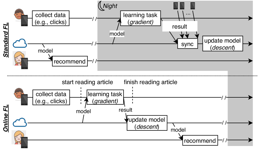
Figure 1. Online FL enables frequent updates without requiring idle-charging-WiFi connected mobile devices.

We fully implemented the server side and the Android client of FLeet . We evaluate the potential of FLeet and show that it can increase the accuracy of a recommendation system (that employs Standard FL) by 2.3$\times$ on average, by performing the same number of updates but in a more timely (online) manner. Even though the learning tasks drain energy directly from the battery of the phone, they consume on average only 0.036% of the battery capacity of a modern smartphone per user per day. We also evaluate the components of FLeet on 40 commercial Android devices, by using popular benchmarks for image classification. Regarding I-Prof, we show that 90% of the learning tasks deviate from a fixed Service Level Objective (SLO) of 3 seconds by at most 0.75 seconds in comparison to 2.7 seconds for the competitor (the profiler of MAUI (Cuervo et al., 2010)). The energy deviation from an SLO of 0.075% battery drop is 0.01% for I-Prof and 0.19% for the competitor. We also show that our staleness-aware learning algorithm (AdaSGD) learns 18.4% faster than its competitor (DynSGD (Jiang et al., 2017)) on heterogeneous data.

2. FLeet

FLeet incorporates two components we consider necessary in any system that has the ambition to provide both, the (a) privacy of FL and (b) the precision of online learning systems. The first component is I-Prof, a lightweight ML-based profiling mechanism that controls the computation time and energy of the learning task by using ML-based estimators. The second component of FLeet is AdaSGD, a new adaptive learning algorithm that tolerates stale updates by automatically adjusting their weight.

2.1. Architectural Overview

Similar to the implementation of Standard FL (Bonawitz et al., 2019), FLeet follows a client-server architecture (Figure 2) where each user hosts a worker and the service provider hosts the server (typically in the cloud). In FLeet, the worker is a library that can be used by any mobile ML-based application (e.g., a news articles application). The model training protocol of FLeet is the following (the numbers refer to Figure 2):

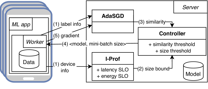
Figure 2. The architecture of FLeet.

1. The worker requests a learning task and sends information regarding the labels of the local data along with information about the state of the mobile device. We introduce the purpose of this information in Steps 2 and 3.

2. I-Prof employs the device information to bound the workload size (i.e., set a mini-batch size bound) that will be allocated to this worker such that the computation time and energy consumption approximate an SLO set by the service provider or negotiated with the user (details in Section 2.2). The mini-batch size is then set as the $min$(mini-batch size bound, local data size).

3. AdaSGD computes a similarity for the requested learning task with past learning tasks in order to adapt to updates with new data (details in Section 2.3).

4. In order to prevent the computation of learning tasks with low or no utility for the learning procedure, the controller checks if both the mini-batch size and the similarity values pass certain thresholds set by the service provider. If the check fails, the request of the worker is rejected, otherwise the controller sends the model parameters and the mini-batch size to the worker and the learning task execution begins (details about setting these thresholds in Section 2.4).

5. Based on the mini-batch size returned by the server, the worker samples from its locally collected data, performs the learning task (i.e., one or multiple local model updates) and sends the result (i.e., the gradient) back to the server. On the server side, AdaSGD updates the model after dynamically adapting this gradient based on its staleness and on its similarity value (details in Section 2.3).

The above protocol maintains the key “privacy-readiness” of Standard FL: the user data never leave the device.

2.2. Workload Bound via Profiling

In Online FL, a mobile device should be able to compute model updates at any time, not only during the night, when the mobile device is idle, charging and connected to WiFi. Therefore, FLeet drops the constraint of Standard FL for high device availability. Hence, the learning task now drains energy directly from the battery of the device. Controlling the impact of a learning task on the user application in terms of energy consumption and computation time becomes crucial. To this end, FLeet incorporates a profiling mechanism that determines the workload size (i.e., the mini-batch size) appropriate for each mobile device.

Best-effort solution.

To highlight the need for a specific profiling tool, we first consider a naive solution in which users process data points until they reach the SLO either in terms of computation time or energy. At this point, a worker sends back the resulting “best-effort” gradient. The service provider cannot decide beforehand whether for a given device, the cost (in terms of energy, time and bandwidth) to download the model, compute and upload the gradient is worth the benefit to the model. Updates computed on very small mini-batch sizes (by weak devices) will perturb the convergence of the overall model, and might even negate the benefit of other workers.

To illustrate this point, consider the experiment of Figure 3. The figure charts the result of training a Convolutional Neural Network on CIFAR10 (Krizhevsky, 2009) under different combinations of “strong” and “weak” workers. The strong workers compute on a mini-batch size of 128 while the weak workers compute on a mini-batch size of 1. We observe that even 2 weak workers are enough to cancel the benefit of distributed learning, i.e., the performance with 10 strong + 2 weak workers is the same as training with a single strong worker.

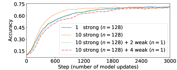
Figure 3. Motivation for lower bounding the mini-batch size. The noise introduced by weak workers (i.e., with small mini-batch sizes) may be detrimental to learning.

One way to avoid this issue could be to drop all the gradients computed on a mini-batch size lower than a given bound or weigh them with a tiny factor according to the size of their underlying mini-batch. This way would however waste the energy required to obtain these gradients. A profiler tool that can estimate the maximum mini-batch size (workload bound) that a worker can compute is necessary for the controller to decide whether to reject the computation request of this worker, before the gradient computation. Unfortunately, existing profiling approaches (Kwon et al., 2013; Chowdhury et al., 2015; Yoon et al., 2012; Hao et al., 2013; Carroll et al., 2010; Chu et al., 2011; Cuervo et al., 2010) are not suitable because they are either relatively inaccurate (see Section 3.3) or they require privileged access (e.g., rooted Android devices) to low-level system performance counters.

I-Prof.

Mobile devices have a significantly lower level of parallelism in comparison with cloud servers. For example, the graphical accelerators of mobile devices generally have 10-20 cores (Arm Mali Graphics Processing Units (GPUs), 2020; Qualcomm, 2020) while the GPUs on a server have thousands of cores (NVIDIA, 2020). Given this low level of parallelism, even a relatively small mini-batch size can fill the processing pipelines. Hence, any additional workload will linearly increase the computation time and the energy consumption. Based on this observation, we built I-Prof, a lightweight profiler specifically designed for Online FL systems. We design I-Prof with three goals in mind: (a) operate effectively with data from a wide range of device types, (b) do so in a lightweight manner, i.e., introduce only a negligible latency to the learning task and (c) rely only on the data available on a stock (non-rooted) Android device.

I-Prof employs an ML-based scheme to capture how the device features affect the computation time and energy consumption of the learning task. I-Prof predicts the largest mini-batch size a device can process while respecting both the time and the energy limits set by the SLO. To this aim, I-Prof uses two predictors, one for computation time and one for energy. Each predictor updates its state with data from the device information sent by the workers.

Designing such predictors is however tricky, as modern mobile phones exhibit a wide range of capabilities. For example, in a matrix multiplication benchmark, Galaxy S6 performs 7.11 Gflops whereas Galaxy S10 performs 51.4 Gflops (Labs, 2020). Figure 4 illustrates this heterogeneity on three different mobile devices by executing successive learning tasks of increasing mini-batch size (“up”). After reaching the maximum value, we let the devices cool down and execute subsequent learning tasks with decreasing mini-batch size (“down”). We present the results for the up-down part with the same color-pattern, except for Honor 10 in Figure 4(b) that we split for highlighting the difference. Figure 4 illustrates that the linear relation changes for each device and for certain devices (Honor 10, Galaxy S7) also changes with the temperature. Note that Honor 10 shows an increased variance at the end of the “up” part (Figure 4(b)) that is attributed to the high temperature of the device. The variance is significantly smaller for the “down” part.

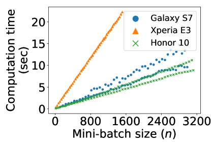
((a))

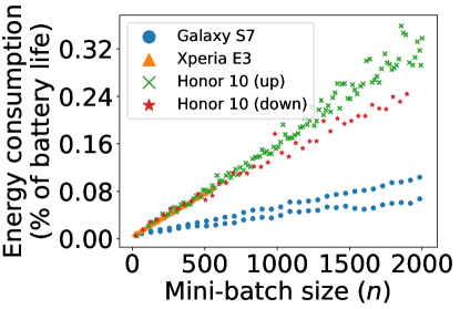
((b))

Figure 4. The linear relation between the computation time and the mini-batch size depends on the specific device, and may even vary for the same device, depending on operation conditions such temperature.

In the following, we describe how I-Prof predicts the mini-batch size ($n$) given a computation time SLO ($t_{SLO}$). The computation time linearly increases with the workload size, i.e., $t_{comp}=\alpha\cdot n$, where $\alpha$ depends on the device and its state. Considering the goal (i.e., $t_{comp}\rightarrow t_{SLO}$), the optimal mini-batch size is predicted as:

(1) $$\hat{n}=\max\left(1,\frac{t_{SLO}}{\hat{\alpha}}\right)$$

I-Prof estimates the slope $\hat{\alpha}$ from the device characteristics and operational conditions using a method that combines linear regression and online passive-aggressive learning (Crammer et al., 2006).

The input to this method is a set of device features based on measurements available through the Android API, namely available memory, total memory, temperature and sum of the maximum frequency over all the CPU cores. However, these features only encode the computing power of a device. For the prediction based on the energy SLO, I-Prof also needs a feature that encodes the energy efficiency of each device. We choose this additional feature as the energy consumption per non-idle CPU time. We show in our evaluation (Section 3.3) that these features achieve our three design goals. Given a vector of device features ($\bm{x}$), and a vector of model parameters (${\bm{\theta}}_{\text{prof}}$), the slope $\hat{\alpha}$ is estimated as $\hat{\alpha}=\bm{x}^{T}{\bm{\theta}}_{\text{prof}}$.

I-Prof uses a cold-start linear regression model for the first request of each user device. We pre-train the cold-start model using ordinary least squares with an offline dataset. This dataset consists of data collected by executing requests from a set of training devices with a mini-batch size increasing from 1 till a value such that the computation time reaches twice the SLO. I-Prof periodically re-trains the cold-start model after appending new data (device features). The training cost is negligible given the small number of features.

Furthermore, I-Prof creates a personalized model for every new device model (e.g., Galaxy S7) and employs it for every following request coming from this particular model. I-Prof bootstraps the new model with the first request (for which the cold-start model is used to estimate the computation time). For all the following learning tasks that result in pairs of ($\bm{x}^{(k)},\alpha^{(k)}$), I-Prof incrementally updates a Passive-Aggressive (PA) model (Crammer et al., 2006) as: ${{\bm{\theta}}_{\text{prof}}^{(k+1)}={\bm{\theta}}_{\text{prof}}^{(k)}+\frac{f^{(k)}}{\left\lVert\bm{x}^{(k)}\right\rVert^{2}}\bm{v}^{(k)}}$ where ${\bm{v}^{(k)}=sign(\alpha^{(k)}-\bm{x}^{(k)\,T}{\bm{\theta}}^{(k)}_{\text{prof}})\bm{x}^{(k)}}$ denotes the update direction, and $f$ the loss function:

(2) $$f({\bm{\theta}}_{\text{prof}},\bm{x},\alpha)=\begin{cases}0&\text{if }|\bm{x}^{T}{\bm{\theta}}_{\text{prof}}-\alpha|\leq\epsilon\\ |\bm{x}^{T}{\bm{\theta}}_{\text{prof}}-\alpha|-\epsilon&\text{otherwise.}\end{cases}$$

The parameter $\epsilon$ controls the sensitivity to prediction error and thereby the aggressiveness of the regression algorithm, i.e., the smaller the value of $\epsilon$ the larger the update for each new data instance (more aggressive).

I-Prof focuses solely on the time and energy spent during an SGD computation. Despite network costs (in particular when transferring models) having also an important impact, they fall outside the scope of this work as one can rely on prior work (Altamimi et al., 2015; Liu and Lee, 2015; Qian et al., 2011) to estimate the time and energy of network transfers within FLeet.

2.3. Adaptive Stochastic Gradient Descent

The server-driven synchronous training of Standard FL is not suitable for Online FL, as the latter requires frequent updates and needs to exploit contributions from all workers, including slow ones (Section 1). Therefore, we introduce AdaSGD, an asynchronous learning algorithm that is robust to stale updates. AdaSGD is responsible for aggregating the gradients sent by the workers and updating the application model (${\bm{\theta}}_{\text{app}}$). Each update takes place after AdaSGD receives $K$ gradients. The aggregation parameter $K$ can be either fixed or based on a time window (e.g., update the model every 1 hour). The model update is:

(3) $${\bm{\theta}}_{\text{app}}^{(t+1)}={\bm{\theta}}_{\text{app}}^{(t)}-\gamma_{t}\sum_{i=1}^{K}\min\left(1,\Lambda(\tau_{i})\cdot\frac{1}{sim(\bm{x}_{i})}\right)\cdot\bm{G}({\bm{\theta}}_{\text{app}}^{(t_{i})},\xi_{i})$$

where $\gamma_{t}$ is the learning rate, $t\in\mathbb{N}$ denotes the global logical clock (or step) of the model at the server (i.e., the number of past model updates) and $t_{i}\leq t$ denotes the logical clock of the model that the worker receives. $\bm{G}({\bm{\theta}}_{\text{app}}^{(t_{i})},\xi_{i})$ is the gradient computed by the client w.r.t the model ${\bm{\theta}}_{\text{app}}^{(t_{i})}$ on the mini-batch $\xi_{i}$ drawn uniformly from the local dataset $\bm{x}_{i}$.

The workers send gradients asynchronously that can result in stale updates. The staleness of the gradient (${\tau_{i}:=t-t_{i}}$) shows the number of model updates between the model pull and gradient push of worker $i$. One option is to directly apply this gradient, at the risk of slowing down or even completely preventing convergence (Jiang et al., 2017; Zhang et al., 2016). The Standard FL algorithm (FedAvg (McMahan et al., 2017)) simply drops stale gradients. However, even if computed on a stale model, the gradient may incorporate potentially valuable information. Moreover, in FLeet, the gradient computation may drain energy directly from the battery of the phone, thus making the result even more valuable. Therefore, AdaSGD utilizes even stale gradients without jeopardizing the learning process, by multiplying each gradient with an additional weight to the learning rate. This weight consists of (a) a dampening factor based on the staleness ($\Lambda(\tau_{i})$) and (b) a boosting factor based on the user’s data novelty ($\frac{1}{sim(\bm{x}_{i})}$), that we describe in the following.

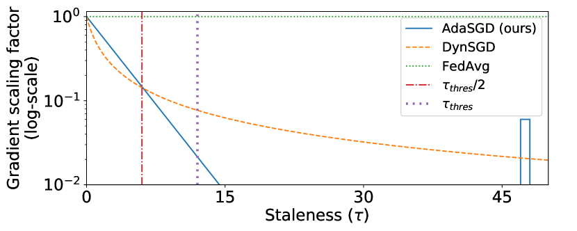
Figure 5. Gradient scaling schemes of SGD algorithms. AdaSGD, proposed in this paper, dampens stale gradients with an exponentially decreasing function ($\Lambda(\tau)$) based on the expected percentage of non-stragglers ($\tau_{\text{thres}}:=s$-th percentile of staleness values), and boosts the gradient of the straggler ($\tau=48$) due to its low similarity ($sim(\bm{x}_{i})$).

Staleness-based dampening.

AdaSGD builds on prior work on staleness-aware learning that has shown promising results (Jiang et al., 2017; Zhang et al., 2016). In order to accelerate learning, AdaSGD relies on a system parameter: the expected percentage of non-stragglers (denoted by $s\%$). We highlight that this value is not a hyperparameter that needs tuning for each ML application but a system parameter that solely depends on the computing and networking characteristics of the workers, while it can be adapted dynamically (Ouyang et al., 2016; Phan et al., 2019). We define the staleness-aware dampening factor $\Lambda(\tau)=e^{-\beta\tau}$, with $\beta$ chosen s.t. ${\frac{1}{\frac{\tau_{\text{thres}}}{2}+1}=e^{-\beta\frac{\tau_{\text{thres}}}{2}}}$ (i.e., the inverse dampening function (Jiang et al., 2017) intersects with our exponential dampening function in $\frac{\tau_{\text{thres}}}{2}$), where $\tau_{\text{thres}}$ is the $s$-th percentile of past staleness values. Figure 5 shows the dampening factor of AdaSGD compared to the inverse dampening function (employed by DynSGD (Jiang et al., 2017)). Our hypothesis is that the perturbation to the learning process introduced by stale gradients, increases exponentially and not linearly with the staleness. We empirically verify the superior performance of our exponential dampening function compared to the inverse in Section 3.2.

As a quantile, $\tau_{\text{thres}}$ is estimated from the staleness distribution. In practice, for the past staleness values to be representative of the actual distribution, an initial bootstrapping phase can employ the dampening factor of DynSGD. After this phase, the service provider can set $s\%$ and deploy AdaSGD. An underestimate of $s\%$ will slow down convergence, whereas an overestimate may lead to divergence. As we empirically observe (Section 3.1), the staleness distribution often has a long tail. In such cases, the best choice of $s\%$ is the one that sets $\tau_{\text{thres}}$ at the beginning of the tail.

Similarity-based boosting.

In the presence of stragglers with large delays (comparing to the mean latency), staleness can grow and drive $\Lambda(\tau)$ close to 0, i.e., almost neglect the gradients of these stragglers. Nevertheless, these gradients may contain valuable information. In particular, they may be computed on data that are not similar to the data used by past gradients. Hence, AdaSGD boosts these gradients by using the following similarity value:

(4) $$sim(\bm{x}_{i})=BC(\bm{LD}(\bm{x}_{i}),\bm{LD}_{global})$$

where $BC$ denotes the Bhattacharyya coefficient (Wikipedia, 2019), and $\bm{LD}$ the label distribution, that captures the importance of each gradient. We choose this coefficient given our constraints ($sim(\bm{x}_{i})\in[0,1]$). For instance, given an application with 4 distinct labels and a local dataset ($\bm{x}_{i}$) that has 1 example with label 0, and 2 examples with label 1: ${\bm{LD}(\bm{x}_{i})=[\frac{1}{3},\frac{2}{3},0,0]}$. The global label distribution ($\bm{LD}_{global}$) is computed on the aggregate number of previously used samples for each label. We highlight that $\bm{LD}$ is not specific to classification ML tasks; for regression tasks, $\bm{LD}$ would involve a histogram, with the length of the $\bm{LD}$ vector being equal to the number of bins instead of the number of classes.

The similarity value essentially captures how valuable the information of the gradient is. For instance, if a gradient is computed on examples of an unseen label (e.g., a very rare animal), then its similarity value is less than 1 (i.e., has information not similar to the current knowledge of the model). For the similarity computation, the server needs only the indices of the labels of the local datasets without any semantic information (e.g., label 3 corresponds to “dogs”).

2.4. Implementation

The server of FLeet is implemented as a web application (deployed on an HTTP server) and the worker as an Android library. The server transfers data with the workers via Java streams by using Kryo (EsotericSoftware, 2020) and Gzip. In total, FLeet accounts 26913 Java LoC, 3247 C/C++ LoC and 1222 Python LoC.

Worker runtime.

We design the worker of our middleware (FLeet) as a library and execute it only when the overlying ML application (Figure 2) is running in the foreground for two main reasons. First, since Android is a UI-interactive operating system, background applications have low priority so their access to system resources is heavily restricted and they are likely to be killed by the operating system to free resources for the foreground running app. Therefore, allowing the worker to run in the background would make its performance very unpredictable and thus impact the predictions of I-Prof. Second, running the worker in the foreground alleviates the impact of collocated (background) workload.

We build our main library for Convolutional Neural Networks in C++ on top of FLeet. We employ (i) the Java Native Interface (JNI) for the server, (ii) the Android NDK for the worker, (iii) an encoding scheme for transferring C++ objects through the java streams, and (iv) a thread-based parallelization scheme for the independent gradient computations of the worker. On recent mobile devices that support NEON (Arm, 2020), FLeet accelerates the gradient computations by using SIMD instructions. We also port a popular deep learning library (DL4J (Deeplearning4j, 2020)) to FLeet, to benefit from its rich ecosystem of ML algorithms. However, as DL4J is implemented in Java, we do not have full control over the resource allocation.

FLeet relies on the developer of the overlying ML application to ensure the performance isolation between the running application and the worker runtime. The worker can execute in a window of low user activity (e.g., while the user is reading an article) to minimize the impact of the overlying ML application on the predictive power of I-Prof.

Resource allocation.

Allocating system resources is a very challenging task given the latency and energy constraints of mobile devices (Mishra et al., 2018; Ding et al., 2019). Our choice of employing only stock Android without root access means we can only control which cores execute the workload on the worker, with no access, for instance, to low-level advanced tuning. Given this limited control and the inherent mobile device heterogeneity, we opt for a simple yet effective scheme for allocating resources.

This scheme schedules the execution only on the “big” cores for ARM big.LITTLE architectures and on all the cores otherwise. In the case of computationally intensive tasks (such as the learning tasks of FLeet), big cores are more energy efficient than LITTLE cores because they finish the computation much faster (Greenhalgh, 2013). Regarding ARMv7 symmetric architectures with 2 and 4 cores that equip older mobile devices, the energy consumption per workload is constant regardless of the number of cores: a higher level of parallelism will consume more energy but the workload will execute faster. For this reason, our allocation policy relies on all the available cores so that we can take advantage of the embarrassingly parallel nature of the gradient computation tasks. For such tasks, we empirically show (Section 3.4) that this scheme outperforms more complex alternatives (Mishra et al., 2018).

Controller thresholds.

In practice, the service provider can adopt various approaches to define the size and similarity thresholds of the controller (Figure 2). One option is A/B testing along with the gradual increase of the thresholds. In particular, the system initializes the thresholds to zero and divides the users into two groups. The first group tests the impact of the mini-batch size and the second the impact of the label similarity. Both groups gradually increase the thresholds until the impact on the service quality is considered acceptable. The server can execute this A/B testing procedure periodically, i.e., reset the thresholds after a time interval. We empirically evaluate the impact of these thresholds on prediction quality in Section 3.5.

3. Evaluation

Our evaluation consists of two main parts. First, in Section 3.1, we evaluate the claim that Online FL holds the potential to deliver better ML performance than Standard FL (Bonawitz et al., 2019) for applications that employ data with high temporality (Section 1). Second, we evaluate in more detail the internal mechanisms of FLeet, namely AdaSGD (Section 3.2), I-Prof (Section 3.3), the resource allocation scheme (Section 3.4) and the controller (Section 3.5).

We deploy the server of FLeet on a machine with an Intel Xeon X3440 with four CPU cores, 16 GiB RAM and 1 Gb Ethernet, on Grid5000 (Grid5000, 2020). The workers are deployed on a total of 40 different mobile phones that we either personally own or belong to the AWS Device Farm (AWS Device Farm, 2020) (Oregon, USA). In Section 3.1, we deploy the worker on a Raspberry Pi 4 as our hashtag recommender is implemented on TensorFlow that does not yet support training on Android devices.

3.1. Online VS Standard Federated Learning

We compare Online with Standard FL on a Twitter hashtag recommender. Tweepy (Tweepy, 2020) enables us to collect around 2.6 million tweets spanning across 13 successive days and located in the west coast of the USA. We preprocess these tweets (e.g., remove automatically generated tweets, remove special symbols) based on (Dhingra et al., 2016). We then divide the data into shards, each spanning 2 days, and divide each shard into chunks of 1 hour. We finally group the data into mini-batches based on the user id.

Our training and evaluation procedure follows an Online FL setup. Our model is a basic Recurrent Neural Network implemented on TensorFlow with 123,330 parameters (Google, 2020b), that predicts the $5$ hashtags with the largest values on the output layer. The model training consists of successive gradient-descent operations, with each gradient derived from a single mini-batch (i.e., sent by a single user). Every day includes 24 mini-batches and thus 24 distinct gradient computations, while each model update uses 1 gradient. For the Online FL setup, the 24 daily updates are evenly distributed (one update every hour). Training uses the data of the previous hour and testing uses the data of the next hour. For the Standard FL setup, the 24 daily updates occur all at once (at the end of the day). Training uses the data of the previous day and testing uses the data of the next day. We highlight that under this setup, the two approaches employ the same number of gradient computations and the difference lies only in the time they perform the model updates. We also compare against a baseline model that always predicts the most popular hashtags (Kowald et al., 2017; Otsuka et al., 2014). We evaluate the model on the data of each chunk and reset the model at the end of each shard.

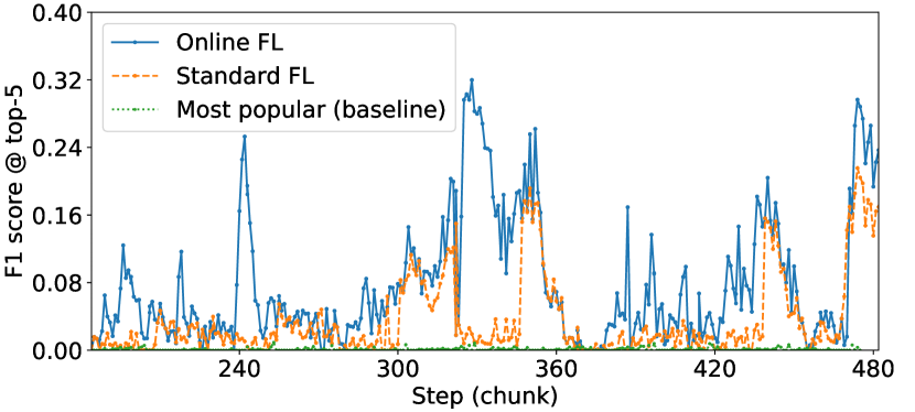
Figure 6. Online FL boosts Twitter hashtag recommendations by an average of 2.3$\times$ comparing to Standard FL.

Quality boost.

For assessing the quality of the hashtag recommender, we employ the F1-score @ top-5 (Kowald et al., 2017; Gong and Zhang, 2016) to capture how many recommendations were used as hashtags (precision) and how many of the used hashtags were recommended (recall). In particular, for each tweet in the evaluation set, we compare the output of the recommender (top-5 hashtags) with the actual hashtags of the tweet, and derive the F1-score. Figure 6 shows that Online FL outperforms Standard FL in terms of F1-score, with an average boost of 2.3$\times$. Online FL updates the model in a more timely manner, i.e., soon after the data generation time, and can thus better predict (higher F1-score) the new hashtags than Standard FL. The performance of the baseline model is quite low as the nature of the data is highly temporal (Kywe et al., 2012).

Energy impact.

We measure the energy impact of the gradient computation on the Raspberry Pi worker. The Raspberry Pi has no screen; nevertheless recent trends in mobile/embedded processor design show that the processor is dominating the energy consumption, especially for compute intensive workloads such as the gradient computation (Halpern et al., 2016). We measure the power consumption of every update of Online FL by executing the corresponding gradient computation 10 times and by taking the median energy consumption. We observe that the power depends on the batch size and increases from 1.9 Watts (idle) to 2.1 Watts (batch size of 1) and to 2.3 Watts (batch size of 100). The computation latency is 5.6 seconds for batch size of 1 and 8.4 for batch size of 100. Across all the updates of Online FL (that employ various batch sizes and result in the quality boost shown in Figure 6), we measure the average, median, $99^{\text{th}}$ percentile and maximum values of the daily energy consumption as 4, 3.3, 13.4 and 44 mWh respectively. Given that most modern smartphones have battery capacities over 11000 mWh, we argue that Online FL imposes a minor energy consumption overhead for boosting the prediction quality.

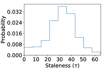
((a))

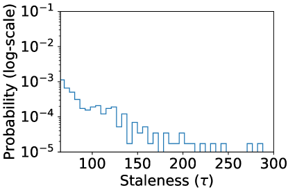
((b))

Figure 7. Staleness distribution of collected tweets follows a Gaussian distribution ($\tau<65$) with a long tail ($\tau>65$).

Staleness distribution.

We study the staleness distribution of the updates on our collected tweets, in order to set our experimental setup for evaluating AdaSGD (Section 3.2). We assume that the round-trip latency per model update (gradient computation time plus network latency) follows an exponential distribution (as commonly done in the distributed learning literature (Mitliagkas et al., 2016; Dutta et al., 2016; Lee et al., 2017; Al-Lawati and Draper, 2020)). The network latency for downloading the model (123,330 parameters) and uploading the gradients is estimated to 1.1 second for 4G LTE and 3.8 seconds for 3G HSPA+ (How fast is 4G?, 2020). We then estimate the average computation latency to be 6 seconds, based on our latency measurements on the Raspberry Pi. Therefore, we choose the exponential distribution with a minimum of $6+1.1=7.1$ seconds and a mean of $\frac{(6+1.1)+(6+3.8)}{2}=8.45$ seconds. Given the exponential distribution for the round-trip latency and the timestamps of the tweets, we observe (in Figure 7) that the staleness follows a Gaussian distribution with a long tail (as assumed in (Zhang et al., 2016)). The long tail is due the presence of certain peak times with hundreds of tweets per second.

Noteworthy, for applications such as our Twitter hashtag recommender where the user activity (and therefore the per-user data creation) is concentrated in time, the difference between Online and Standard FL in terms of communication overhead (due to the gradient-model exchange) is negligible. For applications where the per-user data creation is spread across the day, the communication overhead of Online FL grows, as each user communicates more often with the server.

3.2. AdaSGD Performance

We now dissect the performance of AdaSGD via an image classification application that involves Convolutional Neural Networks (CNNs). We choose this benchmark due to its popularity for the evaluation of SGD-based approaches (Zhang et al., 2016; Abadi et al., 2016b; Chilimbi et al., 2014; Zhao et al., 2018; McMahan et al., 2017; Kang et al., 2017). We employ multiple scenarios involving various staleness distributions, data distributions, and a noise-based differentially private mechanism.

Image classification setup.

We implement the models shown in Table 1 in FLeet to classify handwritten characters and colored images. We use three publicly available datasets: MNIST (Lecun, 1998), E-MNIST (Cohen et al., 2017) and CIFAR-100 (Krizhevsky, 2009). MNIST consists of 70,000 examples of handwritten digits (10 classes) while E-MNIST consists of 814,255 examples of handwritten characters and digits (62 classes). CIFAR-100 consists of 60,000 colour images in 100 classes, with 600 images per class. We perform min-max scaling as a pre-processing step for the input features.

We split each dataset into training / test sets: 60,000 / 10,000 for MNIST, 697,932 / 116,323 for E-MNIST and 50,000 / 10,000 for CIFAR-100. Unless stated otherwise, we set the aggregation parameter $K$ (Section 2.3) to 1 (for maximum update frequency), the mini-batch size to 100 examples (Neyshabur et al., 2015), the $\epsilon$ (the Passive-Aggressive parameter) to 0.1 and the learning rate to $15*10^{-4}$ for CIFAR-100, $8*10^{-4}$ for E-MNIST, and $5*10^{-4}$ for MNIST.

Since the training data present on mobile devices are typically collected by the users based on their local environment and usage, both the size and the distribution of the training data will typically heavily vary among users. Given the terminology of statistics, this means that the data are not Independent and Identically Distributed (non-IID). Following recent work on FL (Wang et al., 2019a; Yurochkin et al., 2019; Wang et al., 2019b; Zhao et al., 2018), we employ a non-IID version of MNIST. Based on the standard data decentralization scheme (McMahan et al., 2017), we sort the data by the label, divide them into shards of size equal to $\frac{60000}{\text{2 * number of users}}$, and assign 2 shards to each user. Therefore, each user will contain examples for only a few labels.

Table 1. CNN parameters.

Dataset	Parameters	Input	Conv1	Pool1	Conv2	Pool2	FC1	FC2	FC3
MNIST	Kernel size Strides	28$\times$28$\times$1	5$\times$5$\times$8 1$\times$1	3$\times$3 3$\times$3	5$\times$5$\times$48 1$\times$1	2$\times$2 2$\times$2	10	–	–
E-MNIST	Kernel size Strides	28$\times$28$\times$1	5$\times$5$\times$10 1$\times$1	2$\times$2 2$\times$2	5$\times$5$\times$10 1$\times$1	2$\times$2 2$\times$2	15	62	–
CIFAR-100	Kernel size Strides	32$\times$32$\times$3	3$\times$3$\times$16 1$\times$1	3$\times$3 2$\times$2	3$\times$3$\times$64 1$\times$1	4$\times$4 4$\times$4	384	192	100

Staleness awareness setup.

To be able to precisely compare AdaSGD with its competitors, we control the staleness of the updates produced by the workers of FLeet. Based on (Zhang et al., 2016) and the shape of the staleness distribution shown in Figure 7, we employ Gaussian distributions for the staleness with two setups: $D1:=\mathcal{N}(\mu=6,\sigma=2)$ and $D2:=\mathcal{N}(\mu=12,\sigma=4)$, to measure the impact of increasing the staleness. We set the expected percentage of non-stragglers ($s\%$) to 99.7%, i.e., $\tau_{\text{thres}}=\mu+3\sigma$. We evaluate the SGD algorithms on FLeet by using commercial Android devices from AWS.

We evaluate the performance of AdaSGD against three learning algorithms: (i) DynSGD (Jiang et al., 2017), a staleness-aware SGD algorithm employing an inverse dampening function (${\Lambda(\tau)=\frac{1}{\tau+1}}$), that AdaSGD builds upon (Section 2.3), (ii) the standard SGD algorithm with synchronous updates (SSGD) that represents the ideal (staleness-free) convergence behaviour, and (iii) FedAvg (McMahan et al., 2017), the standard staleness-unaware SGD algorithm that is based on gradient averaging.

Staleness-based dampening.

Figure 8 depicts that AdaSGD outperforms the alternative learning schemes for the non-IID version of MNIST. As expected, the staleness-free scenario (SSGD) delivers the fastest (ideal) convergence, whereas the staleness-unaware FedAvg diverges. The comparison between the two staleness-aware algorithms (DynSGD and AdaSGD) shows that our solution (AdaSGD) better adapts the dampening factor to the noise introduced by stale gradients (Section 2.3). AdaSGD reaches 80% accuracy 14.4% faster than DynSGD for $D1$ and 18.4% for $D2$. Figure 8 also depicts the impact of staleness on DynSGD and AdaSGD. We observe that the larger the staleness, the slower the convergence of both algorithms. The advantage of AdaSGD over DynSGD grows with the amount of staleness as the larger amount of noise gives more leeway to AdaSGD to benefit from its superior dampening scheme.

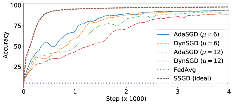
Figure 8. Impact of staleness on learning.

Similarity-based boosting.

We evaluate the effectiveness of the similarity-based boosting property of AdaSGD (Section 2.3) in the case of long tail staleness (Figure 7). We employ the non-IID MNIST dataset, $D1$ (thus $\tau_{\text{thres}}$ is 12) and set the staleness to $4\cdot\tau_{\text{thres}}=48$ for all the gradients computed on data with class 0. This setup essentially captures the case where a particular label is only present in stragglers. Figure 9(a) shows that AdaSGD incorporates the knowledge from class 0 much faster than DynSGD.

Figure 9(b) shows the CDF for the dampening values used to weight the gradients of Figure 9(a). We mark the two points of interest regarding the $\tau_{\text{thres}}$ by vertical lines (as also shown in Figure 5). If AdaSGD had no similarity-based boosting, all updates related to class 0 would almost not be taken into account, as they would be nullified by the exponential dampening function, therefore leading to a model with poor predictions for this class. Given the low class similarity of the learning tasks involving class 0, AdaSGD boosts their dampening value. The second vertical line denotes the staleness value ($\frac{\tau_{\text{thres}}}{2}=6$) for which AdaSGD and DynSGD give the same dampening value ($0.14$). The slope of each curve at this point indicates that the dampening values for DynSGD are more concentrated whereas the ones for AdaSGD are more spread around this value.

((a))

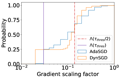
((b))

Figure 9. Impact of long tail staleness on learning.

IID data.

Although data are more likely to be non-IID in an FL environment, the data collected on mobile devices might in some cases be IID. We thus benchmark AdaSGD under two additional datasets (E-MNIST and CIFAR-100) with the staleness following $D2$. Figure 10 shows that our observations from Figure 8 hold also with IID data. As with non-IID data, FedAvg diverges also in the IID setting, and AdaSGD performs better than DynSGD on both datasets.

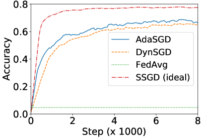
((a)) E-MNIST

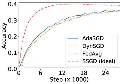
((b)) CIFAR-100

Figure 10. Staleness awareness with IID data.

Differential privacy.

Differential privacy (Dwork et al., 2014) is a popular technique for privacy-preserving FL with formal guarantees (Bonawitz et al., 2017). We thus compare AdaSGD against DynSGD in a differentially private setup by perturbing the gradients as in (Abadi et al., 2016b). We keep the previous setup (IID data with $D2$) and employ the MNIST dataset. Based on (Wu et al., 2017), we fix the probability $\delta=1/N^{2}=\frac{1}{60000^{2}}$ and measure the privacy loss ($\epsilon$) with the moments accountant approach (Abadi et al., 2016b) given the sampling ratio ($\frac{\text{mini-batch size}}{N}=\frac{100}{60000}$), the noise amplitude, and the total number of iterations.

Figure 11 demonstrates that the advantage of AdaSGD over DynSGD also holds in the differentially private setup. A better privacy guarantee (i.e., smaller $\epsilon$) slows down the convergence for both staleness-aware learning schemes.

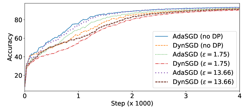
Figure 11. Staleness awareness with differential privacy.

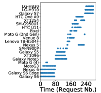
((a)) Request schedule

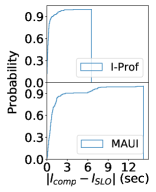
((b)) error CDF

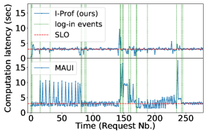
((c)) Request computation time

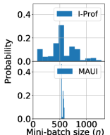
((d)) Profiler output

Figure 12. I-Prof outperforms MAUI and drives the computation time closer to the SLO.

3.3. I-Prof Performance

We compare I-Prof against the profiler of MAUI (Cuervo et al., 2010), a mobile device profiler aiming to identify the most energy-consuming parts of the code and offload them to the cloud. MAUI predicts the energy by using a linear regression model (similar to the global model of I-Prof) on the number of CPU cycles ($\hat{E}=\theta_{0}\cdot n$), to essentially capture how the size of the workload affects the energy (as in (Mittal et al., 2012)). We adapt the profiler of MAUI to our setup by replacing the CPU cycles with the mini-batch size for two main reasons. First, our workload has a static code path so the number of CPU cycles on a particular mobile device is directly proportional to the mini-batch size. Second, measuring the number of executed CPU cycles requires root access that is not available on AWS.

We bootstrap the global model of I-Prof and the model of MAUI by pre-training on a training dataset. To this end, we use 15 mobile devices in AWS (that are different from the ones used for the rest of the experiments), assign them learning tasks with increasing mini-batch size until the computation time becomes 2 times the SLO, and collect their device information for each task. We rely on the same methodology to evaluate energy consumption but use only 3 mobile devices in our lab, as AWS prohibits energy measurements.

For testing, we use a different set of 20 commercial mobile devices in AWS, each performing requests for the image classification application (on MNIST), starting at different timestamps (log-in events) as shown in Figure 12(a). In order to ensure a precise comparison with MAUI, we add a round-robin dispatcher to the profiler component which alternates the requests from a given device between I-Prof and MAUI.

Computation time SLO.

Figure 12(b) shows that I-Prof largely outperforms MAUI in terms of deviation from the computation time SLO. 90% of approximately 280 learning tasks deviate from an SLO of 3 seconds by at most 0.75 seconds with I-Prof and 2.7 seconds with MAUI. This is the direct outcome of our design decisions. First, I-Prof adds dynamic features (e.g., the temperature of the device) to train its global model (Section 2.2). As a result, the predictions are more accurate for the first request of each user. Second, I-Prof uses a personalized model for each device that reduces the error (deviation from the SLO) with every subsequent request (Figure 12(c)). Figure 12(d) shows that the personalized models of I-Prof are able to output a wider range of mini-batch sizes that better match the capabilities of individual devices. On the contrary, MAUI relies on a simple linear regression model which has acceptable accuracy for its use-case but is inefficient when profiling heterogeneous mobile devices.

Energy SLO.

To assess the ability of I-Prof to also target the energy SLO, we use the same setup as for the computation time, except on 5 mobile devices. We configure I-Prof with a significantly smaller error margin, $\epsilon=6*10^{-5}$ (Equation 2), because the linear relation (capture by $\alpha$ as defined in Section 2.2) is significantly smaller for the energy than for the computation time (as shown in Figure 4).

Figure 13 shows that I-Prof significantly outperforms MAUI in terms of deviation from the energy SLO. 90% of 36 learning tasks deviate from an SLO of 0.075% battery drop by at most 0.01% for I-Prof and 0.19% for MAUI. The observation that I-Prof is able to closely match the latency SLO, while MAUI suffers from huge deviations, holds for the energy too. The PA personalized models are able to quickly adapt to the state of the device as opposed to the linear model of MAUI that provides biased predictions.

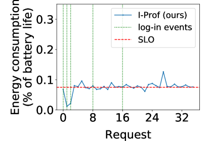
((a)) I-Prof (ours)

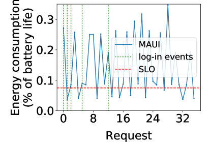
((b)) MAUI

Figure 13. I-Prof outperforms MAUI and drives the energy closer to the SLO.

3.4. Resource Allocation

We evaluate our resource allocation scheme (Section 2.4) and compare it against CALOREE (Mishra et al., 2018) which is a state of the art resource manager for mobile devices. The goal of CALOREE is to optimize resource allocation in order for the workload execution to meet its predefined deadline while minimizing the energy consumption. To this end, CALOREE profiles the target device by running the workload with different resource configurations (i.e., number of cores, core frequency). Since FLeet executes on non-rooted mobile devices, we can only adapt the number of big/little cores (but not their frequencies). By varying the number of cores allocated to our workload (i.e., gradient computation), we obtain the energy consumption of each possible configuration. From these configurations, CALOREE only selects those with the optimal energy consumption (the lower convex hull) which are packed in the so called performance hash table (PHT).

CALOREE on new devices.

In their thorough evaluation, the authors of CALOREE used the same device for training and running the workloads. Therefore, we first benchmark the performance of CALOREE when running on new devices. We employ Galaxy S7 to collect the PHT and set the mini-batch size that I-Prof gives for a latency SLO of 3 seconds (Section 3.3). We then run this workload with CALOREE on different mobile devices, as shown in Table 2.

The performance of CALOREE degrades significantly when running on a different device than the one used for training. The first line of Table 2 shows the baseline error when running on the same device. The error increases more than 6$\times$ for a device with similar architecture and the same vendor (Galaxy S8) and more than 32$\times$ for a device of similar architecture but different vendor (Honor 9 and 10). This significant increase for the error is due to the heterogeneity of the mobile devices which make PHTs not applicable across different device models.

Table 2. Performance of CALOREE (Mishra et al., 2018) on new devices.

Running device	Deadline error (%)
Galaxy S7	1.4
Galaxy S8	9
Honor 9	46
Honor 10	255

CALOREE vs FLeet.

We evaluate the resource allocation scheme of FLeet by comparing it to the ideal environment for CALOREE, i.e., training and running on the same device (a setup nevertheless difficult to achieve in FL with millions of devices). Following the setup used for the energy SLO evaluation (Section 3.3), we employ 5 devices and fix the size of the workload (mini-batch size) based on the output of I-Prof. In particular we set the mini-batch size to 280, 4320, 6720, 5280, 1200 for the devices shown in Figure 14 respectively. We set the deadline of CALOREE either equal or double than the computation latency of FLeet. We take 10 measurements and report on the median, 10th and 90th percentile.

Figure 14 shows the fact that in the ideal environment for CALOREE and even with double the time budget (giving more flexibility to CALOREE), FLeet has comparable energy consumption. Since gradient computation is a compute intensive task with high temporal and spacial cache locality, the configuration changes performed by CALOREE negatively impact the execution time and cancel any energy saved by its advanced resource allocation scheme. Additionally, the fewer configuration knobs available on non-rooted Android devices limit the full potential of CALOREE.

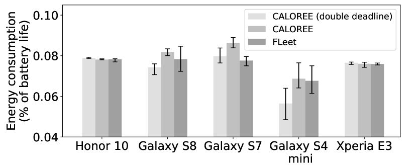
Figure 14. Resource allocation of FLeet vs. CALOREE.

3.5. Learning Task Assignment Control

The controller of FLeet employs a threshold to prune learning tasks and thus control the trade-off between the cost of the gradient computations and the model prediction quality. This threshold can be based either on the mini-batch size or on the similarity values (Figure 2). To evaluate this trade-off, we employ non-IID MNIST with the mini-batch size following a Gaussian distribution $\mathcal{N}(\mu=100,\sigma=33)$ (based on the distribution of the output of I-Prof shown in Figure 12(d)), and set the threshold to the $n-\text{th}$ percentile of the past values. Figure 15 illustrates that a threshold on the mini-batch size is more effective in pruning the less useful gradient computations than a threshold on the similarity. Figure 15(a) shows that even dropping up to 39.2% of the gradients (with the smallest mini-batch size) has a negligible impact on the accuracy (less than 2.2%). Figure 15(b) shows that one can drop 17% of the most similar gradients with an accuracy impact of 4.8%.

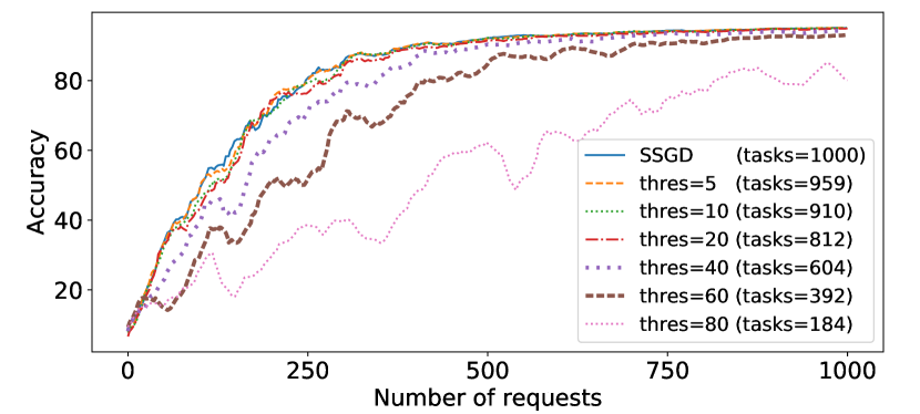
((a)) Based on mini-batch size

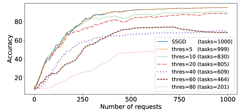
((b)) Based on similarity

Figure 15. Threshold-based pruning.

4. Related Work

Distributed ML.

Adam (Chilimbi et al., 2014) and TensorFlow (Abadi et al., 2016a) adopt the parameter server architecture (Li et al., 2014) for scaling out on high-end machines, and typically require cross-worker communication. FLeet also follows the parameter server architecture, by maintaining a global model on the server. However, FLeet avoids cross-worker communication, which is impractical for mobile workers due to the device churn.

A common approach for large-scale ML is to control the amount of staleness for boosting convergence (Cui et al., 2014; Qiao et al., 2018). In Online FL, staleness cannot be controlled as this would impact the model update frequency. The workers perform learning tasks asynchronously with end-to-end latencies that can differ significantly (due to device heterogeneity and network variability) or even become infinite (user disconnects).

Petuum (Xing et al., 2015) and TensorFlow handle faults (worker crashes) by checkpointing and repartitioning the model across the workers whenever failures are detected. In a setting with mobile devices, such failures may appear very often, thus increasing the overhead for checkpointing and repartitioning. FLeet does not require any fault-tolerance mechanism for its workers, as from a global learning perspective, they can be viewed as stateless.

Federated learning.

In order to minimize the impact on mobile devices, Standard FL algorithms (Jeong et al., 2018; McMahan et al., 2017; Smith et al., 2017; Bonawitz et al., 2019) require the learning task to be executed only when the devices are idle, plugged in, and on a free wireless connection. However, in Section 3.1, we have shown that these requirements may drastically impact the performance of some applications. Noteworthy, techniques for reducing the communication overhead (Jeong et al., 2018) or increasing the robustness against adversarial users (Damaskinos et al., 2018, 2019), are orthogonal to the online characteristic so they can be adapted for AdaSGD, and plugged into FLeet.

Performance prediction for mobile devices.

Estimating the computation time or energy consumption of an application running on a mobile device is a very broad area of research. Existing approaches (Kwon et al., 2013; Chowdhury et al., 2015; Yoon et al., 2012; Hao et al., 2013; Carroll et al., 2010; Chu et al., 2011) target multiple applications generally executing on a single device. They typically benchmark the device or monitor hardware and OS-level counters that require root access. In contrast, FLeet targets a single application executing in the same way across a large range of devices. I-Prof poses a negligible overhead, as it employs features only from the standard Android API to enable Online FL, and requires no benchmarking of new devices. I-Prof is designed to make predictions for unknown devices.

Neurosurgeon (Kang et al., 2017) is a scheduler that minimizes the end-to-end computation time of inference tasks (whereas FLeet focuses on training tasks), by choosing the optimal partition for a neural network and offloading computations to the cloud. The profiler of Neurosurgeon only uses workload-specific features (e.g., number of filters or neurons) to estimate computation time and energy, and ignores device-specific features. By contrast, mobile phones, as targeted by I-Prof , exhibit a wide range of device-specific characteristics that significantly impact their latency and energy consumption (Figure 4).

Systems such as CALOREE (Mishra et al., 2018) and LEO (Mishra et al., 2015) profile mobile devices under different system configurations and train an ML model to determine the ones that minimize the energy consumption. They rely on a control loop to switch between these configurations such that the application does not miss the preset deadline. Due to the restrictions of the standard Android API, the available knobs are limited in our setup. For our application (i.e., gradient computation), we show that a simple resource allocation scheme (Section 2.4) is preferable even in comparison with an ideal execution model.

5. Concluding Remarks

This paper presented FLeet, the first system that enables online ML at the edge. FLeet employs I-Prof, a new ML-based profiler which determines the ML workload that each device can perform within predefined energy and computation time SLOs. FLeet also makes use of AdaSGD, a new staleness-aware learning algorithm that is optimized for Online FL. We showed the performance of I-Prof and AdaSGD on commercial Android devices with popular benchmarks. I-Prof can be used for any iterative computation with embarrassingly-parallel CPU-bound tasks while AdaSGD is specific to gradient-descent and thus ML applications. In our performance evaluation we do not focus on network and scalability aspects that are orthogonal to our work and addressed in existing literature. We also highlight that transferring the label and device information (Figure 2) poses a negligible network overhead compared to transferring the relatively large FL learning models. Finally, addressing biases is an important problem even in cloud-based online ML (not only FL) that we also do not address in this work. For Online FL we arguably need to keep some of these biases (e.g., recommend more politics to people that wake up earlier). Of course diversity is also crucial.

Although we believe FLeet to represent a significant advance for online learning at the edge, there is still room for improvement. First, for the energy prediction, I-Prof requires access to the CPU usage that is considered as a security flaw on some Android builds and thus not exposed to all applications. In this case, I-Prof requires a set of additional permissions that belong to services from Android Runtime. Second, the transfer of the label distribution from the worker to the server introduces a potential privacy leakage. However, we highlight that the server has access only to the indices of the labels and not their values. In this paper, we focus on the protection of the input features and mention the possibility to deactivate the similarity-based boosting feature of AdaSGD in the case that this leakage is detrimental. We plan to investigate noise addition techniques for bounding this leakage (Dwork et al., 2014) in our future work. Finally, theoretically proving the convergence of AdaSGD is non-trivial due to the unbounded staleness and the non Independent and Identically Distributed (non-IID) datasets among the workers. In this respect, a dissimilarity assumption similar to (Li et al., 2018) may facilitate the derivation of the proof.

6. Acknowledgments

We thank Dr. Sonia Ben-Mokhtar, our shepherd Prof. Christine Julien, our colleagues from the DCL laboratory at EPFL and the anonymous reviewers, for their helpful feedback. This work was supported by the EPFL-Inria International Lab and by the French ANR project PAMELA n. ANR-16-CE23-0016.

References

- (1)
- Abadi et al. (2016a) Martín Abadi, Paul Barham, Jianmin Chen, Zhifeng Chen, Andy Davis, Jeffrey Dean, Matthieu Devin, Sanjay Ghemawat, Geoffrey Irving, Michael Isard, et al. 2016a. TensorFlow: A system for large-scale machine learning. In OSDI. 265–283.
- Abadi et al. (2016b) Martín Abadi, Andy Chu, Ian Goodfellow, H Brendan McMahan, Ilya Mironov, Kunal Talwar, and Li Zhang. 2016b. Deep learning with differential privacy. In CCS. ACM, 308–318.
- Al-Lawati and Draper (2020) Haider Al-Lawati and Stark C Draper. 2020. Gradient Delay Analysis in Asynchronous Distributed Optimization. In ICASSP. IEEE, 4207–4211.
- Altamimi et al. (2015) Majid Altamimi, Atef Abdrabou, Kshirasagar Naik, and Amiya Nayak. 2015. Energy cost models of smartphones for task offloading to the cloud. TETC 3, 3 (2015), 384–398.
- Arm (2020) Arm. 2020. SIMD ISAs — Neon. https://developer.arm.com/architectures/instruction-sets/simd-isas/neon.
- Arm Mali Graphics Processing Units (GPUs) (2020) Arm Mali Graphics Processing Units (GPUs) 2020. https://developer.arm.com/ip-products/graphics-and-multimedia/mali-gpus.
- AWS Device Farm (2020) AWS Device Farm 2020. https://aws.amazon.com/device-farm/.
- Bonawitz et al. (2019) Keith Bonawitz, Hubert Eichner, Wolfgang Grieskamp, Dzmitry Huba, Alex Ingerman, Vladimir Ivanov, Chloe Kiddon, Jakub Konecny, Stefano Mazzocchi, H Brendan McMahan, et al. 2019. Towards Federated Learning at Scale: System Design. Proceedings of the 2nd SysML Conference (2019).
- Bonawitz et al. (2017) Keith Bonawitz, Vladimir Ivanov, Ben Kreuter, Antonio Marcedone, H Brendan McMahan, Sarvar Patel, Daniel Ramage, Aaron Segal, and Karn Seth. 2017. Practical secure aggregation for privacy-preserving machine learning. In CCS. ACM, 1175–1191.
- Carroll et al. (2010) Aaron Carroll, Gernot Heiser, et al. 2010. An Analysis of Power Consumption in a Smartphone. In USENIX ATC, Vol. 14. Boston, MA, 21–21.
- Chen et al. (2018) Fei Chen, Zhenhua Dong, Zhenguo Li, and Xiuqiang He. 2018. Federated Meta-Learning for Recommendation. arXiv preprint arXiv:1802.07876 (2018).
- Chilimbi et al. (2014) Trishul M Chilimbi, Yutaka Suzue, Johnson Apacible, and Karthik Kalyanaraman. 2014. Project Adam: Building an Efficient and Scalable Deep Learning Training System. In OSDI, Vol. 14. 571–582.
- Chowdhury et al. (2015) Shaiful Alam Chowdhury, Luke N Kumar, Md Toukir Imam, Mohomed Shazan Mohomed Jabbar, Varun Sapra, Karan Aggarwal, Abram Hindle, and Russell Greiner. 2015. A system-call based model of software energy consumption without hardware instrumentation. In IGSC. 1–6.
- Chu et al. (2011) David Chu, Nicholas D Lane, Ted Tsung-Te Lai, Cong Pang, Xiangying Meng, Qing Guo, Fan Li, and Feng Zhao. 2011. Balancing energy, latency and accuracy for mobile sensor data classification. In SenSys. ACM, 54–67.
- Cohen et al. (2017) Gregory Cohen, Saeed Afshar, Jonathan Tapson, and André van Schaik. 2017. EMNIST: an extension of MNIST to handwritten letters. arXiv preprint arXiv:1702.05373 (2017).
- Crammer et al. (2006) Koby Crammer, Ofer Dekel, Joseph Keshet, Shai Shalev-Shwartz, and Yoram Singer. 2006. Online passive-aggressive algorithms. JMLR 7, Mar (2006), 551–585.
- Crushh (2017) Crushh. 2017. Average text message length. https://crushhapp.com/blog/k-wrap-it-up-mom.
- Cuervo et al. (2010) Eduardo Cuervo, Aruna Balasubramanian, Dae-ki Cho, Alec Wolman, Stefan Saroiu, Ranveer Chandra, and Paramvir Bahl. 2010. MAUI: making smartphones last longer with code offload. In MobiSys. ACM, 49–62.
- Cui et al. (2014) Henggang Cui, James Cipar, Qirong Ho, Jin Kyu Kim, Seunghak Lee, Abhimanu Kumar, Jinliang Wei, Wei Dai, Gregory R Ganger, Phillip B Gibbons, et al. 2014. Exploiting Bounded Staleness to Speed Up Big Data Analytics. In USENIX ATC. 37–48.
- Damaskinos et al. (2019) Georgios Damaskinos, El Mahdi El Mhamdi, Rachid Guerraoui, Arsany Guirguis, and Sébastien Louis Alexandre Rouault. 2019. Aggregathor: Byzantine machine learning via robust gradient aggregation. In Conference on Machine Learning and Systems (SysML / MLSys).
- Damaskinos et al. (2018) Georgios Damaskinos, El Mahdi El Mhamdi, Rachid Guerraoui, Rhicheek Patra, Mahsa Taziki, et al. 2018. Asynchronous Byzantine Machine Learning (the case of SGD). In ICML. 1153–1162.
- Deeplearning4j (2020) Deeplearning4j. 2020. DL4J. https://deeplearning4j.org/.
- Dhingra et al. (2016) Bhuwan Dhingra, Zhong Zhou, Dylan Fitzpatrick, Michael Muehl, and William W Cohen. 2016. Tweet2vec: Character-based distributed representations for social media. arXiv preprint arXiv:1605.03481 (2016).
- Ding et al. (2019) Yi Ding, Nikita Mishra, and Henry Hoffmann. 2019. Generative and Multi-Phase Learning for Computer Systems Optimization. In ISCA (Phoenix, Arizona) (ISCA ’19). Association for Computing Machinery, New York, NY, USA, 39–52. https://doi.org/10.1145/3307650.3326633
- Dutta et al. (2016) Sanghamitra Dutta, Viveck Cadambe, and Pulkit Grover. 2016. Short-dot: Computing large linear transforms distributedly using coded short dot products. In NIPS. 2100–2108.
- Dwork et al. (2014) Cynthia Dwork, Aaron Roth, et al. 2014. The algorithmic foundations of differential privacy. Foundations and Trends® in Theoretical Computer Science 9, 3–4 (2014), 211–407.
- EsotericSoftware (2020) EsotericSoftware. 2020. Kryo. https://github.com/EsotericSoftware/kryo/.
- Gong and Zhang (2016) Yuyun Gong and Qi Zhang. 2016. Hashtag Recommendation Using Attention-Based Convolutional Neural Network. In IJCAI. 2782–2788.
- Google (2020a) Google. 2020a. TensorFlow - Federated Learning. https://www.tensorflow.org/federated/federated_learning.
- Google (2020b) Google. 2020b. Tensorflow text classification. https://www.tensorflow.org/tutorials/text/text_classification_rnn#create_the_model
- government (2018) US government. 2018. California Consumer Privacy Act of 2018 (CCPA). https://leginfo.legislature.ca.gov/faces/billTextClient.xhtml?bill_id=201720180AB375.
- Greenhalgh (2013) P Greenhalgh. 2013. big. LITTLE Technology: The Future of Mobile. ARM, White paper (2013).
- Grid5000 (2020) Grid5000. 2020. Grid5000. https://www.grid5000.fr/.
- Halpern et al. (2016) Matthew Halpern, Yuhao Zhu, and Vijay Janapa Reddi. 2016. Mobile cpu’s rise to power: Quantifying the impact of generational mobile cpu design trends on performance, energy, and user satisfaction. In HPCA. IEEE, 64–76.
- Hao et al. (2013) Shuai Hao, Ding Li, William GJ Halfond, and Ramesh Govindan. 2013. Estimating mobile application energy consumption using program analysis. In ICSE. IEEE Press, 92–101.
- Hard et al. (2018) Andrew Hard, Kanishka Rao, Rajiv Mathews, Swaroop Ramaswamy, Françoise Beaufays, Sean Augenstein, Hubert Eichner, Chloé Kiddon, and Daniel Ramage. 2018. Federated learning for mobile keyboard prediction. arXiv preprint arXiv:1811.03604 (2018).
- How fast is 4G? (2020) How fast is 4G? 2020. https://www.4g.co.uk/how-fast-is-4g/.
- Jeong et al. (2018) Eunjeong Jeong, Seungeun Oh, Hyesung Kim, Jihong Park, Mehdi Bennis, and Seong-Lyun Kim. 2018. Communication-Efficient On-Device Machine Learning: Federated Distillation and Augmentation under Non-IID Private Data. arXiv preprint arXiv:1811.11479 (2018).
- Jiang et al. (2017) Jiawei Jiang, Bin Cui, Ce Zhang, and Lele Yu. 2017. Heterogeneity-aware Distributed Parameter Servers. In SIGMOD. 463–478.
- Kang et al. (2017) Yiping Kang, Johann Hauswald, Cao Gao, Austin Rovinski, Trevor Mudge, Jason Mars, and Lingjia Tang. 2017. Neurosurgeon: Collaborative intelligence between the cloud and mobile edge. In ASPLOS. 615–629.
- Konečnỳ et al. (2016) Jakub Konečnỳ, H Brendan McMahan, Daniel Ramage, and Peter Richtárik. 2016. Federated optimization: distributed machine learning for on-device intelligence. arXiv preprint arXiv:1610.02527 (2016).
- Kowald et al. (2017) Dominik Kowald, Subhash Chandra Pujari, and Elisabeth Lex. 2017. Temporal effects on hashtag reuse in twitter: A cognitive-inspired hashtag recommendation approach. In WWW. 1401–1410.
- Krizhevsky (2009) Alex Krizhevsky. 2009. Cifar dataset. https://www.cs.toronto.edu/~kriz/cifar.html.
- Kwon et al. (2013) Yongin Kwon, Sangmin Lee, Hayoon Yi, Donghyun Kwon, Seungjun Yang, Byung-Gon Chun, Ling Huang, Petros Maniatis, Mayur Naik, and Yunheung Paek. 2013. Mantis: Automatic performance prediction for smartphone applications. In USENIX ATC. 297–308.
- Kywe et al. (2012) Su Mon Kywe, Tuan-Anh Hoang, Ee-Peng Lim, and Feida Zhu. 2012. On recommending hashtags in twitter networks. In International Conference on Social Informatics. Springer, 337–350.
- Labs (2020) Primate Labs. 2020. Matrix multiplication benchmark. https://browser.geekbench.com.
- Lecun (1998) Yann Lecun. 1998. MNIST dataset. http://yann.lecun.com/exdb/mnist/.
- Lee et al. (2017) Kangwook Lee, Maximilian Lam, Ramtin Pedarsani, Dimitris Papailiopoulos, and Kannan Ramchandran. 2017. Speeding up distributed machine learning using codes. IEEE Transactions on Information Theory 64, 3 (2017), 1514–1529.
- Li et al. (2014) Mu Li, David G Andersen, Jun Woo Park, Alexander J Smola, Amr Ahmed, Vanja Josifovski, James Long, Eugene J Shekita, and Bor-Yiing Su. 2014. Scaling distributed machine learning with the parameter server. In OSDI. 583–598.
- Li et al. (2018) Tian Li, Anit Kumar Sahu, Manzil Zaheer, Maziar Sanjabi, Ameet Talwalkar, and Virginia Smith. 2018. Federated optimization for heterogeneous networks. arXiv preprint arXiv:1812.06127 (2018).
- Liu and Lee (2015) Yan Liu and Jack YB Lee. 2015. An empirical study of throughput prediction in mobile data networks. In GLOBECOM. IEEE, 1–6.
- McMahan et al. (2017) Brendan McMahan, Eider Moore, Daniel Ramage, Seth Hampson, and Blaise Aguera y Arcas. 2017. Communication-Efficient Learning of Deep Networks from Decentralized Data. In AISTATS. 1273–1282.
- media (2013) Vox media. 2013. NSA’s PRISM. https://www.theverge.com/2013/7/17/4517480/nsa-spying-prism-surveillance-cheat-sheet.
- media (2018) Vox media. 2018. The Facebook and Cambridge Analytica scandal. https://www.vox.com/policy-and-politics/2018/3/23/17151916/facebook-cambridge-analytica-trump-diagram.
- Mishne et al. (2013) Gilad Mishne, Jeff Dalton, Zhenghua Li, Aneesh Sharma, and Jimmy Lin. 2013. Fast data in the era of big data: Twitter’s real-time related query suggestion architecture. In SIGMOD. ACM, 1147–1158.
- Mishra et al. (2018) Nikita Mishra, Connor Imes, John D Lafferty, and Henry Hoffmann. 2018. CALOREE: Learning control for predictable latency and low energy. ASPLOS 53, 2 (2018), 184–198.
- Mishra et al. (2015) Nikita Mishra, Huazhe Zhang, John D Lafferty, and Henry Hoffmann. 2015. A probabilistic graphical model-based approach for minimizing energy under performance constraints. ASPLOS 50, 4 (2015), 267–281.
- Mitliagkas et al. (2016) Ioannis Mitliagkas, Ce Zhang, Stefan Hadjis, and Christopher Ré. 2016. Asynchrony begets momentum, with an application to deep learning. In Annual Allerton Conference on Communication, Control, and Computing. IEEE, 997–1004.
- Mittal et al. (2012) Radhika Mittal, Aman Kansal, and Ranveer Chandra. 2012. Empowering developers to estimate app energy consumption. In MobiCom. ACM, 317–328.
- Neyshabur et al. (2015) Behnam Neyshabur, Ruslan R Salakhutdinov, and Nati Srebro. 2015. Path-sgd: Path-normalized optimization in deep neural networks. In NIPS. 2422–2430.
- Nishio and Yonetani (2019) Takayuki Nishio and Ryo Yonetani. 2019. Client selection for federated learning with heterogeneous resources in mobile edge. In ICC. IEEE, 1–7.
- NVIDIA (2020) NVIDIA. 2020. CUDA GPUs — NVIDIA Developer. https://developer.nvidia.com/cuda-gpus.
- Otsuka et al. (2014) Eriko Otsuka, Scott A Wallace, and David Chiu. 2014. Design and evaluation of a twitter hashtag recommendation system. In IDEAS. 330–333.
- Ouyang et al. (2016) Xue Ouyang, Peter Garraghan, David McKee, Paul Townend, and Jie Xu. 2016. Straggler detection in parallel computing systems through dynamic threshold calculation. In AINA. IEEE, 414–421.
- Phan et al. (2019) Tien-Dat Phan, Guillaume Pallez, Shadi Ibrahim, and Padma Raghavan. 2019. A new framework for evaluating straggler detection mechanisms in mapreduce. TOMPECS 4, 3 (2019), 1–23.
- Qian et al. (2011) Feng Qian, Zhaoguang Wang, Alexandre Gerber, Zhuoqing Mao, Subhabrata Sen, and Oliver Spatscheck. 2011. Profiling resource usage for mobile applications: a cross-layer approach. In MobiSys. ACM, 321–334.
- Qiao et al. (2018) Aurick Qiao, Abutalib Aghayev, Weiren Yu, Haoyang Chen, Qirong Ho, Garth A Gibson, and Eric P Xing. 2018. Litz: Elastic framework for high-performance distributed machine learning. In USENIX ATC. 631–644.
- Qualcomm (2020) Qualcomm. 2020. Adreno™ Graphics Processing Units. https://developer.qualcomm.com/software/adreno-gpu-sdk/gpu.
- request (2016) Text request. 2016. Average text messages per day. https://www.textrequest.com/blog/how-many-texts-people-send-per-day/.
- Ryffel et al. (2018) Theo Ryffel, Andrew Trask, Morten Dahl, Bobby Wagner, Jason Mancuso, Daniel Rueckert, and Jonathan Passerat-Palmbach. 2018. A generic framework for privacy preserving deep learning. arXiv preprint arXiv:1811.04017 (2018).
- S20.ai (2020) S20.ai. 2020. S20.ai. https://www.s20.ai/.
- Smith et al. (2017) Virginia Smith, Chao-Kai Chiang, Maziar Sanjabi, and Ameet S Talwalkar. 2017. Federated multi-task learning. In NIPS. 4424–4434.
- Snips (2020) Snips. 2020. Snips - Using Voice to Make Technology Disappear. https://snips.ai/.
- Statista (2018) Statista. 2018. Percentage of all global web pages served to mobile phones from 2009 to 2018. https://www.statista.com/statistics/241462/global-mobile-phone-website-traffic-share/.
- Tweepy (2020) Tweepy 2020. https://tweepy.readthedocs.io/en/latest/.
- Union (2016) European Union. 2016. Regulation 2016/679 of the European Parliament and of the Council of 27 April 2016 on the protection of natural persons with regard to the processing of personal data and on the free movement of such data, and repealing Directive 95/46/EC (GDPR). https://eur-lex.europa.eu/legal-content/EN/TXT/PDF/?uri=CELEX:32016R0679.
- Wang et al. (2019b) Shiqiang Wang, Tiffany Tuor, Theodoros Salonidis, Kin K Leung, Christian Makaya, Ting He, and Kevin Chan. 2019b. Adaptive federated learning in resource constrained edge computing systems. IEEE Journal on Selected Areas in Communications 37, 6 (2019), 1205–1221.
- Wang et al. (2019a) Zhibo Wang, Mengkai Song, Zhifei Zhang, Yang Song, Qian Wang, and Hairong Qi. 2019a. Beyond inferring class representatives: User-level privacy leakage from federated learning. In INFOCOM. IEEE, 2512–2520.
- Wikipedia (2019) Wikipedia. 2019. Bhattacharyya coefficient. https://en.wikipedia.org/wiki/Bhattacharyya_distance.
- Wu et al. (2017) Xi Wu, Fengan Li, Arun Kumar, Kamalika Chaudhuri, Somesh Jha, and Jeffrey Naughton. 2017. Bolt-on differential privacy for scalable stochastic gradient descent-based analytics. In SIGMOD. 1307–1322.
- Xing et al. (2015) Eric P Xing, Qirong Ho, Wei Dai, Jin-Kyu Kim, Jinliang Wei, Seunghak Lee, Xun Zheng, Pengtao Xie, Abhimanu Kumar, and Yaoliang Yu. 2015. Petuum: A New Platform for Distributed Machine Learning on Big Data. In KDD. 1335–1344.
- Yang et al. (2018) Timothy Yang, Galen Andrew, Hubert Eichner, Haicheng Sun, Wei Li, Nicholas Kong, Daniel Ramage, and Françoise Beaufays. 2018. Applied federated learning: Improving google keyboard query suggestions. arXiv preprint arXiv:1812.02903 (2018).
- Yoon et al. (2012) Chanmin Yoon, Dongwon Kim, Wonwoo Jung, Chulkoo Kang, and Hojung Cha. 2012. AppScope: Application Energy Metering Framework for Android Smartphone Using Kernel Activity Monitoring. In USENIX ATC, Vol. 12. 1–14.
- Yurochkin et al. (2019) Mikhail Yurochkin, Mayank Agarwal, Soumya Ghosh, Kristjan Greenewald, Nghia Hoang, and Yasaman Khazaeni. 2019. Bayesian Nonparametric Federated Learning of Neural Networks. In ICML. 7252–7261.
- Zhang et al. (2016) Wei Zhang, Suyog Gupta, Xiangru Lian, and Ji Liu. 2016. Staleness-aware async-sgd for distributed deep learning. In IJCAI. 2350–2356.
- Zhao et al. (2018) Yue Zhao, Meng Li, Liangzhen Lai, Naveen Suda, Damon Civin, and Vikas Chandra. 2018. Federated learning with non-iid data. arXiv preprint arXiv:1806.00582 (2018).