Neutron star inner crust: effects of rotation and magnetic fields

Abstract

We study the role of the pasta phases on the properties of rotating and magnetized neutron stars. In order to investigate such systems, we make use of two different relativistic mean-field unified inner-crust–core equations of state, with a different density dependence of the symmetry energy, and an inner-crust computed within a Thomas-Fermi calculation. Special attention is given to the crust-core transition density, and the pasta phases effects on the global properties of stars. The effects of strong magnetic fields and fast rotation are computed by solving the Einstein-Maxwell equations self-consistently, taking into account anisotropies induced by the centrifugal and the Lorentz force. The location of the magnetic field neutral line and the maximum of the Lorentz force on the equatorial plane are calculated. The conditions under which they fall inside the inner crust region are discussed. We verified that models with a larger symmetry energy slope show more sensitivity to the variation of the magnetic field. One of the maxima of the Lorentz force, as well as the neutral line, and for a certain range of frequencies, fall inside the inner crust region. This may have consequences in the fracture of the crust, and may help explain phenomena associated with star quakes.

I Introduction

Neutron stars (NS) are not only extremely dense objects, but they are known to be associated with strong magnetic fields, and fast rotation as well. At present, it is commonly accepted that the huge range of densities inside NS can be naturally divided into several regions. Typically, the neutron star structure can be divided into an outer crust, an inner crust and a core. The outer crust region of neutron stars has an equation of state relatively well-known Baym et al. (1971); Haensel and Pichon (1994); Rüster et al. (2006). The same is not true for the inner crust. This region of the star begins when neutrons start dripping out of the nuclei at densities of about $\rho_{{\rm drip}}\sim 4.3\times 10^{11}$ g/cm³. As a result, the inner crust is formed by very neutron-rich nuclei, immersed in a gas of neutrons and electrons. Heavy clusters, the pasta phases, form due to the competition between the nuclear and Coulomb forces Ravenhall et al. (1983); Pais and Stone (2012); Pais and Providência (2016); Watanabe et al. (2005). This may affect the cooling of the proton neutron star.

Pulsars rotate extremely fast, which is related to their formation Lorimer (2008). As the star core collapses, its rotation rate increases as a result of conservation of angular momentum, hence, pulsars rotate up to several hundred times per second. In the case of millisecond pulsars, they are thought to achieve such high speeds because they are gravitationally bound in a binary system with another star. During part of their life, matter flows from the companion star to the pulsar. Over time, the impact of the accreted matter spins up the pulsar’s rotation.

In addition, classes of neutron stars known as magnetars have strong surface magnetic fields that span the range $\sim 10^{12-15}$ G. Such fields are usually estimated from observations of the star’s period, and period derivative. One expects to find even stronger magnetic fields inside these stars. According to the virial theorem, which gives an upper estimate for the magnetic field inside neutron stars, they can possess stronger central magnetic fields, of the order of $\sim 10^{18}$ G Lai and Shapiro (1991); Cardall et al. (2001).

The main objective of the present work is to understand how the distribution of the poloidal magnetic field lines affect the inner crust of a neutron star. Moreover, we want precisely to identify the thickness of the crust and the position of the poloidal neutral line with respect to the crust, taking as reference an unified equation of state, and allowing for the symmetry energy to vary. The knowledge of the size and position of the crust is important to understand its possible role in the stabilization of the magnetic field and the low frequency quasi-periodic oscillations (QPO) associated with magnetar flares Steiner and Watts (2009); Gabler et al. (2013); Sotani et al. (2013); Deibel et al. (2014); Sotani et al. (2019).

It has been suggested that QPO observed in the decay tails of magnetar flares result from seismic vibrations from neutron stars. Some of these oscillations may be confined to the crust, in particular the low frequency ones, and, in this case, they are perfect probes of the crust EoS, as discussed in Steiner and Watts (2009). The frequency of these modes is directly related with both the thickness of the crust, and the density-dependence of the symmetry energy Sotani et al. (2013); Deibel et al. (2014); Sotani et al. (2019). Another possible interpretation is the association of QPO to magneto-elastic modes Gabler et al. (2013).

Recently, the evolution of the magnetic field structure during the late stage of a proto-neutron star has been studied Lander et al. (2020). It was shown that the structure of the magnetic field is similar in a hot and cold NS, the poloidal component of the field being stronger than the toroidal one. Instabilities may originate a large release of the magnetic energy, but then it is difficult to explain the strong magnetic fields that many magnetars have. The authors suggest that one of the possible mechanisms to stabilize the magnetic field is the solidification of the crust, starting at the crust-core transition. The formation of a solid crust would give rise to elastic forces that would avoid the development of magnetic field instabilities, and a fast decay of the magnetic field. In the present work, using a realistic unified EoS, we will show that the neutral line of the poloidal field, i.e. the region where instabilities develop, may, in fact, fall in the crust region for a rotating star. As it will be discussed, this result is sensitive to the density-dependence of the symmetry energy.

We will, therefore, concentrate our attention on the inner crust-core transition, and will not investigate the outer crust and transition to the inner crust of a strongly magnetized star. Several studies have already shown the important effects of the magnetic field on the outer crust and neutron drip line Potekhin and Chabrier (2013); Chamel et al. (2012, 2015); Stein et al. (2016). In Ref. Chatterjee et al. (2015), the authors have shown that including magnetic field effects in the EoS did not affect much the magnetized neutron star structure, therefore, in the following, we consider a non-magnetized EoS.

In order to describe the neutron star interior, the complete stellar matter EoS will be constructed by taking a standard EoS for the outer crust Baym et al. (1971), with an adequate inner crust EoS that matches the outer crust EoS at the neutron drip line, and the core EoS at the crust-core transition density Pais and Providência (2016). Between the neutron drip density and the crust-core transition density, we employ an inner crust EoS, that we have determined from a Thomas-Fermi calculation for the NL3 family Pais and Providência (2016), with the inclusion of the $\omega\rho$ meson coupling terms. There, the authors addressed the effect of the nonlinear $\omega\rho$ coupling terms on the crust-core transition density and pressure, and on the macroscopic properties of hadronic stars. We will also consider that the magnetic field affects the extension of the inner crust, as proposed in Fang et al. (2016, 2017a, 2017b); Chen (2017). The complete EoS will be used as input to determine the star properties, such as the mass and radius, from the integration of the Einstein-Maxwell equations, in order to obtain both rotating and magnetized stellar models Bonazzola et al. (1993); Bocquet et al. (1995); Franzon et al. (2016a, b).

Pasta phases impact not only the structure of NS, but also may affect their rotation behavior, and the magnetic field distribution. The effects of rotation and strong magnetic fields in the inner crust region, where the pasta phases appear, are going to be analysed, for two model with different slopes of the symmetry energy. For this purpose, we are going to use the Lorene C++ library for numerical relativity to self-consistently study the effects of strong magnetic fields and rotation on neutron stars. We will solve numerically the coupled Maxwell-Einstein equations by means of a pseudo-spectral method, taking into consideration the anisotropy of the energy-momentum tensor due to the magnetic field, and also the effects of the centrifugal force induced by rotation.

If the NS has a poloidal field with closed lines inside, instabilities will appear in the neighborhood of the neutral line characterized by a zero magnetic field Markey and Tayler (1973); Lander and Jones (2011), and a mixed poloidal-toroidal configuration will stabilize the NS Haskell et al. (2008); Lander and Jones (2009, 2011); Pili et al. (2017); Uryu et al. (2019). However, the relative magnitude of each field component depends on the boundary conditions imposed on the magnetic field Haskell et al. (2008); Lander and Jones (2009), and these will certainly depend on the properties of matter at the NS surface. In this paper, we want to address this issue, and the localization of the neutral line of the poloidal magnetic field relative to the crust of the NS will be determined. The structure of the paper is the following: in Sec. II, we review the formalism, in Sec. III, the results are presented, and, finally, in Sec. IV some conclusions are drawn.

II Description of Magnetized and Rotating Neutron Stars

In this section, we review the formalism introduced in Refs. Bonazzola et al. (1993) and Bocquet et al. (1995), upon which the LORENE code is based.

Assuming Maximum-Slice Quasi-Isotropic (MSQI) coordinates, stationarity and axisymmetry, the metric tensor reads

$$\begin{split}\mathrm{d}s^{2}=g_{\mu\nu}\mathrm{d}x^{\mu}x^{\nu}=&-N^{2}\mathrm{d}t^{2}+A^{2}(\mathrm{d}r^{2}+r^{2}\mathrm{d}\theta^{2})\\ &+B^{2}r^{2}\sin^{2}\theta(\mathrm{d}\phi-N^{\phi}\mathrm{d}t)^{2}\end{split}\quad,$$ (1)

with $N(r,\theta)$, $A(r,\theta)$, $B(r,\theta)$ and $N^{\phi}(r,\theta)$ function only of $(r,\theta)$.

We only consider stars with poloidal magnetic fields. In this case, the magnetic vector potential $A_{\mu}$ has components $A_{\mu}=\left(A_{t},0,0,A_{\phi}\right)$. Note that in Ref. Frieben and Rezzolla (2012), the authors constructed toroidal magnetic fields with the choice $A_{\mu}=(0,A_{r},A_{\theta},0)$.

One important question about magnetic field in neutron stars is its decay due to dissipation. Hence, stationary models of neutron stars in magnetic fields require a separation of dynamical and dissipative timescales, encoded in an assumption of infinite conductivity (magnetic fields are ’frozen in’ and carried with the fluid, a common assumption in astrophysics). This assumption is exceedingly well justified for neutron star matter, since the ohmic dissipation timescale is larger than the age of the universe and, therefore, the electric current in the fluid would not suffer ohmic decay Goldreich and Reisenegger (1992). Therefore, we assume infinite conductivity inside the stars. In this case, the magnetic flux $BR^{2}$ ($R$ being the stellar radius) is conserved, and the electric field as measured by the co-moving observer is zero. As a result, we find the relation between the magnetic vector components:

$$A_{t}=-\Omega A_{\phi}+C\quad,$$ (2)

with $\Omega$ the rotation velocity of the star, and $C$ a constant that determines the total electric charge of the star.

The energy-momentum conservation equation $\mathsf{\nabla_{\mu}T^{\mu\nu}=0}$ gives an equation of stationary motion for the fluid with magnetic field

$$\frac{1}{\mathcal{E}+P}\frac{\partial\,P}{\partial x_{i}}+\frac{\partial\,\ln\,N}{\partial x_{i}}-\frac{\ln\,{\rm{\Gamma}}}{\partial x_{i}}+\frac{F^{i\nu}\,j_{\nu}}{\mathcal{E}+P}=0\quad,$$ (3)

with the spatial coordinates $x_{i}=(r,\theta)$. The first term in Eq. (3) corresponds to the purely matter contribution, the second represents the gravitational potential, the third accounts for the centrifugal effects due to rotation, and the last one is the Lorentz force ($f^{\mu}=F^{\mu\nu}\,j_{\nu}$) induced by magnetic fields, which, in our case, are generated by the four-electric current $j_{\nu}$. Since $A_{\mu}=(A_{t},0,0,A_{\phi})$, then $j_{\nu}=(j_{t},0,0,j_{\phi})$, which comes from the assumption of circularity condition. In other words, there are not meridional currents.

Eq. (3) is the relativistic version of the Euler equation. One can show, by taking the rotational, that the Lorentz term in Eq. (3) can be written as

$$\frac{\partial M}{\partial x_{i}}=\frac{F^{i\nu}\,j_{\nu}}{\mathcal{E}+P}=\left(\frac{j^{\phi}-\rm{\Omega}\,j^{t}}{\mathcal{E}+P}\right)\frac{\partial A_{\phi}}{\partial x_{i}}\,.$$ (4)

Note that Eq.(4) represents also the integrability condition of Eq.(3). The term in parenthesis in Eq. (4) can be a constant, or a function of the magnetic vector potential, $g\left(A_{\phi}\right)$. The arbitrary function $M$ can then be chosen such that:

$$\frac{\partial M}{\partial A_{\phi}}=g(A_{\phi})\quad.$$ (5)

In other words,

$$M=M(A_{\phi}(r,\theta))=\int^{A_{\phi}}_{0}g(u)\,du\quad.$$ (6)

The function $g(u)$ is called the current function, and $M$ is the magnetic potential. Here, the magnetic star models are obtained by assuming a constant value for the dimensionless current function, also referred to as current function amplitude (CFA), and denoted by $k_{0}$. In Ref. Bocquet et al. (1995), other choices for $g(u)$ were considered, other than constants functions, but the general conclusions remain the same.

For higher values of the current function, the magnetic field in the star increases proportionally. In addition, $\mathsf{k_{0}}$ is related to the macroscopic electric current via:

$$j^{\phi}={\rm\Omega}\,j^{t}+(\mathcal{E}+P)\,k_{0}\quad,$$ (7)

which is obtained relating Eq. (5) with Eq. (4). Here, $\mathcal{E}$ is the energy density and $P$ is the pressure.

Finally, the integral form of the equation of motion for a fluid in the presence of magnetic fields, Eq. (3), reads:

$$H(r,\theta)+\ln\,N(r,\theta)-\ln\,{\rm{\Gamma(r,\theta)}}\,+M(r,\theta)=const.\quad,$$ (8)

where $M$ is the magnetic potential, see Eq. (6), and $H$ is the dimensionless log-enthalpy (also called pseudo-enthalpy or heat function) defined as

$$H(P)=\int_{0}^{P}\frac{\mathrm{d}P^{\prime}}{\mathcal{E}(P^{\prime})+P^{\prime}}\quad,$$ (9)

which can be cast in terms of the specific enthalpy $\mathsf{h}$

$$h(P)=\frac{\mathcal{E}(P)+P}{m_{b}\,n_{b}}\quad,$$ (10)

as

$$H(P):=\ln\,h(P)=\ln\,\left(\frac{\mu}{m_{b}}\right)\quad,$$ (11)

where $m_{B}=939$ MeV is the baryonic mass, and $\mu$ the baryonic chemical potential.

III Results

In the following, we present the main results of our study. We consider the effect of the magnetic field on the NS crust for a non-rotating star in Sec. III.1, and, for a rotating star, in Sec. III.2.

III.1 Magnetised neutron stars

As already discussed in Ref. Fang et al. (2017a), the presence of strong magnetic fields originates a region, at the boundary between the inner crust and the core, where homogeneous and non-homogeneous matter (matter with the presence of clusters) coexist – the extended crust – identified by the densities $\rho_{1}$ and $\rho_{2}$ (cf. Fig. 1). We shall denote the radii that correspond to each of these densities as $R_{1}$ and $R_{2}$, respectively. In this notation, the thickness of the extended crust is defined as $\Delta R_{t}=R_{1}-R_{2}$, whilst the total size of the crust is given by the difference $\Delta R_{2}=R-R_{2}$ (with $R$ being the coordinate radius of the star). The difference $\Delta R_{1}=R-R_{1}$ corresponds to the size of the crust without the extended region.

Figure 1: (Color online) The extended crust region. The densities $\rho_{1}$ and $\rho_{2}$ define the boundaries of this region.

For the region between the surface and the boundary defined by $R_{1}$ and the density $\rho_{1}$, which coincides with the crust-core transition of a non-magnetized star, we take the EoS of non-magnetized matter. In Fang et al. (2017b), it has been shown that the magnetic field does not affect much the value of $R_{1}$, and the results of de Lima et al. (2013) concerning the inner crust seem to indicate that the structure of the pasta phases inside $R_{1}$ are not influenced by the magnetic field, if the intensity of the field satisfies $B<10^{18}$ G, as expected in the crust region. The authors of de Lima et al. (2013) did not consider the possibility that at densities above $\rho_{1}$ new non-homogeneous regions would exist, as calculated in Fang et al. (2017b), using a dynamical spinodal approach. For the region bounded by $\rho_{1}$ and $\rho_{2}$ in Fig. 1, we will take results of Refs. Fang et al. (2017a, b) to define the location of the non-homogeneous regions, since presently no other results are available that identify these regions.

We consider two models which only differ in the isovector properties: NL3$\omega\rho$ with the symmetry energy slope $L=55$ and 88 MeV at saturation Pais and Providência (2016). These values lie at the average and top limit obtained in Oertel et al. (2017) for the symmetry energy slope at saturation from constraints for nuclear properties and neutron star observations, $L=58.7\pm 28.1$MeV.

Figure 2: (Color online) Effect of the magnetic field on the total size of the crust $\Delta R_{2}$ (top), on the crust without its extension, $\Delta R_{1}$, (middle), and on the extended region, $\Delta R_{t}$ (bottom). Full lines correspond to the model with $L=55$ MeV, whilst dashed lines are for the $L=88$ MeV model. The colours red, blue and green correspond to baryon masses $1.2\mathrm{M}_{\odot}$,$1.5\mathrm{M}_{\odot}$ and $1.8\mathrm{M}_{\odot}$, respectively.

In order to study the effects of the magnetic field on the star crust, we first analyze how the three quantities, $\Delta R_{1}$, $\Delta R_{2}$ and $\Delta R_{t}$, vary with the radial component of the magnetic field measured at the surface (poles), $B_{s}$. These results are presented in Figure 2 for stars with baryon masses 1.2, 1.4 and 1.8 $M_{\odot}$. On the top panel, we show how the size of the crust is affected by the presence of the magnetic field. We note that for $B_{s}=0$, the results for the two models considered do not differ much from each other in comparison with the case where $B_{s}\neq 0$. However, a difference does exist, as discussed in Vidaña et al. (2009), where it was shown that the larger the slope $L$, the smaller the transition density to the core. This, in turn, may reflect itself on the thickness of the crust: in Grill et al. (2014), it was found that a thinner crust corresponds to a larger $L$, when comparing NL3 ($L=118$ MeV) with NL3$\omega\rho$ with $L=55$ MeV.

On the other hand, a much greater difference is verified for $B_{s}\neq 0$. This is because the value $\rho_{2}$, which defines the crust size, depends on the proton fraction value considered. It was shown in Ducoin et al. (2008) that the proton fraction at the crust-core transition is determined by the slope of symmetry energy, the smaller the $L$ the larger the proton fraction. A similar conclusion was drawn in Grill et al. (2012) for the average proton fraction at the inner crust. Therefore, even though both models predict the same properties for symmetric nuclear matter, they will respond differently with the inclusion of the magnetic field due to their different symmetry energy properties. As a result, the model with $L=88$ MeV shows a much bigger sensitivity to the increase of the magnetic field. The reason lies in the fact that, for densities below saturation density, the fraction of protons is smaller for larger values of $L$, and, therefore, more sensitive to a given value of the magnetic field. It is also clear that the smaller the star mass, the larger the effect of the magnetic field.

Figure 3: (Color online) Normalised $R_{1}$, $R_{2}$ and $R$ as a function the polar angle, $\theta$. Full lines correspond to the model with $L=55$ MeV, whilst dashed lines are for the $L=88$ MeV model. The colours red, blue and green correspond to baryon masses $1.2\mathrm{M}_{\odot}$,$1.5\mathrm{M}_{\odot}$ and $1.8\mathrm{M}_{\odot}$, respectively. In each panel, the results obtained with $B_{s}=4.4\times 10^{16}$ G are divided by the corresponding value at $B_{s}=0$ (notice that $R_{2}(B=0)=R_{1}(B=0)$). See text for more details.

Figure 4: (Color online) Baryon density as function of the radial coordinate. The top panel corresponds to $L=55$ MeV whilst the bottom one corresponds to $L=88$ MeV. The colours red, blue and green correspond to baryon masses $1.2\mathrm{M}_{\odot}$,$1.5\mathrm{M}_{\odot}$ and $1.8\mathrm{M}_{\odot}$, respectively. The vertical bands correspond to the transition zone at the crust-core transition.

In the middle panel of Figure 2, it is shown how the size of the crust without the extended zone varies with the magnetic field. Here, the overall trend is a reduction on the size of the region, as the magnetic field increases. Again we note that the model with the larger $L$ is more affected by the increase of the magnetic field, a conclusion that can also be reached by looking at the bottom panel of the same figure, where we present the behavior of the extended crust alone. It is important to note that this behavior is not monotonic, which is a consequence of the discrete feature of the Landau levels introduced by the magnetic field Fang et al. (2017a).

Concerning Fig. 2, some comments are in order: a) there is a large increase of the crust size when the magnetic field increases from 0 to 4.4$\times 10^{15}$ G, but the size of the crust is practically the same for 4.4$\times 10^{15}<B<4.4\times 10^{16}$ G; b) the effect of the magnetic field is much stronger if the model has a large symmetry energy slope; c) stars with smaller masses are more strongly affected.

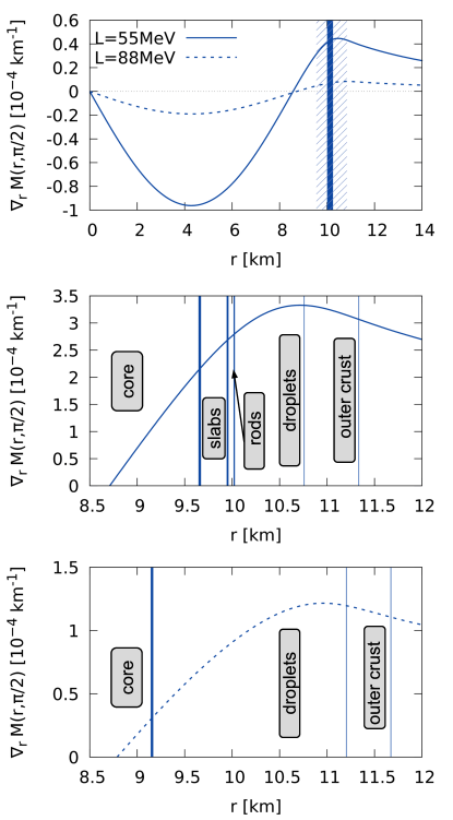
Figure 5: (Color online) Gradient of the magnetic potential as function of the radial coordinate for a $M_{b}=1.5\mathrm{M}_{\odot}$ star with $B_{s}=4.4\times 10^{16}$ G. Full lines correspond to the model with $L=55$ MeV, whilst dashed lines are for the $L=88$ MeV model. The two bottom panels show in more detail the region inside the crust, and the transition between the different pasta phases is signaled.

In Figure 3, we have used the results obtained with the stronger magnetic field intensity ($B_{s}=4.41\times 10^{16}$ G at the surface’s pole) to show how the width of the crust varies along the polar angle $\theta$. We have normalized the curves with the values obtained with $B=0$: for both $R_{1}$ and $R_{2}$, we divided the values obtained with $B_{s}=4.41\times 10^{16}$ G by the corresponding values (i.e. same mass and same $L$) obtained at $B=0$. Since the values $\rho_{1}$ and $\rho_{2}$ do not have any spatial dependency, the results that we observe here are only consequence of the overall deformation of the star induced by the magnetic field. In fact, the way the crust is deformed is quite similar to the deformation of the radius (i.e., coordinate radius) of the star itself, as shown on the bottom panel of the same figure, where the radius $R$ of the star is plotted versus the polar angle. Nonetheless, it becomes clear from Figure 3 that the effect of the magnetic field is much stronger in the $L=88$ MeV model: the difference between the equatorial and polar radii is larger; and the extended crust extends much more into the interior of the star. As discussed before, the magnetic field has a stronger effect on the width of the crust of the less massive star: for the 1.2 $M_{\odot}$ star, the ratio between the equatorial radius is $\approx 5\%$ larger then the polar radius, while for the 1.4 and 1.8 $M_{\odot}$ stars, this difference is $\approx 2-3\%$. It is also interesting to notice that the reduction of the radius at the pole is stronger than its increase at the equator. This is also true for the thickness of the crust. The middle panel shows that the location of the transition of the extended crust-core is shifted towards the interior of the star for the model with $L=88$ MeV, and the star with the smallest mass. This shift is larger at the equator, going up to more than 5% (15%) for the model with $55$ MeV (88 MeV). At the pole, it is not more than 1% for the $L=55$ MeV model, but rises to above 10% for the $L=88$ MeV model.

This is also evident in Figure 4, where we plot the profile of each star that we have considered and, in each of them, we identify the extended zone, the region delimited by $R_{2}$ and $R_{1}$. By doing this, we observe that the extended crust, which is itself a consequence of the inclusion of the magnetic field, is much bigger for the model with the larger $L$.

We next analyze how the magnetic field potential varies inside the star, and we discuss the localization of the points where its gradient, proportional to the Lorentz force, is extreme and zero.

On the top panel of Fig. 5, we plot the radial component of the gradient of the magnetic potential measured along the plane $\theta=0$ as a function of the radial coordinate. This quantity gives us the shape of the radial component of the Lorentz force inside the star, since $\bm{F_{L}}\sim\nabla M\left(r,\theta\right)$. At the equator, the gradient of the magnetic potential function is zero at the neutral line of the poloidal magnetic field Lander and Jones (2011). For polar angles close to the equator, the Lorentz force verifies a sign change inside the star, as discussed in Franzon et al. (2017), because the lines of field are closed. It was shown in Lander and Jones (2011), where the authors have studied instabilities in NS with poloidal magnetic fields, that the most unstable perturbations develop around the neutral line.

We wanted to ascertain whether the neutral line coincides with the extended crust region, which should be taken into account when one considers strong magnetic fields. For the models considered, we verified that that does not occur, and, in fact, we obtained the neutral line at $r=R_{n}$, with $R_{n}/R\sim 0.8$, as predicted in Lander and Jones (2011). It has, however, been shown that stability in a magnetized star is attained with both a poloidal and a toroidal component, with the last one embedded inside the region defined by the poloidal closed lines Haskell et al. (2008); Lander and Jones (2009); Uryu et al. (2019). We have included in Table 1 the position of the neutral line $R_{n}$, and the extension of the crust $R_{2}$ and $R_{1}$, as well as the NS radius $R$, for stars with masses 1.2, 1.4 and 1.8 $M_{\odot}$ described by models with $L=55$ and $L=88$ MeV, and the surface magnetic field $B_{s}=4.41\times 10^{15}$G. In the next section, we will discuss the effect of rotation on the neutral line.

Table 1: The position of the inner crust boundaries $R_{1}$ and $R_{2}$, the NS radius $R$, and the neutral line $R_{n}$ measured along the equatorial plane, for different values of the surface magnetic field, $B_{s}$, and for stars with masses 1.2, 1.4 and 1.8 $M_{\odot}$, and described by models with $L=55$ and $L=88$ MeV. Note: $B^{*}=4.41\times 10^{15}$G.

$L$ (MeV)	Mb $(\mathrm{M}_{\odot})$	$R_{1}$ (km)	$R_{2}$ (km)	$R$ (km)	$R_{n}$ (km)
$B_{s}=B^{*}$
55	1.2	9.987	9.752	11.79	8.660
	1.5	10.14	9.944	11.59	8.640
	1.8	10.15	9.991	11.36	8.522
88	1.2	10.60	9.067	12.25	8.946
	1.5	10.64	9.402	11.96	8.820
	1.8	10.59	9.545	11.65	8.632
$B_{s}=5\,B^{*}$
55	1.2	10.06	9.729	11.83	8.691
	1.5	10.17	9.907	11.62	8.658
	1.8	10.19	9.955	11.38	8.536
88	1.2	10.72	9.131	12.30	8.982
	1.5	10.74	9.444	11.99	8.842
	1.8	10.65	9.573	11.67	8.646
$B_{s}=10\,B^{*}$
55	1.2	10.17	9.873	11.94	8.775
	1.5	10.25	10.01	11.69	8.711
	1.8	10.24	10.02	11.43	8.576
88	1.2	10.98	9.267	12.44	9.084
	1.5	10.91	9.528	12.07	8.905
	1.8	10.77	9.625	11.73	8.688

Besides the neutral line, the Lorentz force has two local extrema inside the NS, one located at the core and the other one in the crust. We may assume that a maximum of the Lorentz force inside the non-homogeneous region of the star may cause more easily matter to fracture or break. On the middle and bottom panels of Fig. 5, we identify the location of the pasta phases in the crust region. In the case of the $L=88$ MeV model, no inner crust configurations besides droplets exist. However, for the $L=55$ MeV, the maximum of the Lorentz force occurs near the region of rod-like configurations, which may be easier to deform. The localization of the transition between pasta phases in our work is only indicative, since they have been obtained in a calculation that considered the possible formation of only five different configurations. In a calculation that allows the appearance of any kind of geometry as in Schneider et al. (2014, 2016); Caplan et al. (2018), the extreme of the Lorentz force would most probably fall in a region of non-spherical pasta phases.

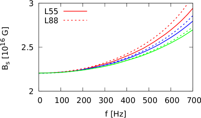
Figure 6: (Color online) Radial component of the magnetic field at the pole surface, $B_{s}$, as function of rotation frequency, $f$, for a fixed magnetic dipole moment. Full lines correspond to the model with $L=55$ MeV, whilst dashed lines are for $L=88$ MeV. The colors red, blue and green correspond to baryon masses $1.2\mathrm{M}_{\odot}$,$1.5\mathrm{M}_{\odot}$ and $1.8\mathrm{M}_{\odot}$, respectively.

III.2 Magnetised and rotating neutron stars

The effects of rotation on the geometry of neutron stars are already well documented Bocquet et al. (1995), the major result being the flatness of the star on the polar regions, an effect similar to that of the polar magnetic fields discussed in the previous section. In Lander and Jones (2011), the authors showed that rotation stabilizes the instabilities developed in neutron stars with a poloidal magnetic field due to perturbations. Here we analyze how the profile of the Lorentz force in the equatorial plane is affected, relatively to the crust, when we take into account the effects of rotation. In particular, we will determine the frequency above which the neutral line does not exist.

It is important to notice that even though we fix the magnitude of the magnetic field on the star by choosing the current function amplitude ($CFA$), which is equivalent to fixing the magnetic dipole moment, the magnitude of the magnetic field measured at the pole surface $B_{s}$ is going to vary as we increase the frequency. This stems from the fact that the angular velocity of the fluid and the magnetic function are related by the fluid’s conservation equation (8). The behavior of $B_{s}$ with the rotation frequency is shown in Fig. 6, where the radial component of the magnetic field at the pole surface is plotted for a fixed CFA value (the one that gives, for each star, a field magnitude of $2.2\times 10^{16}$ G when there is no rotation), using the two models of the present study, and considering stars with masses 1.2, 1.4 and 1.8 $M_{\odot}$. We conclude that larger magnetic field intensities are attained for the smaller mass stars, and with a larger symmetry energy slope. This happens because the proton fraction is bigger for the model with the larger $L$.

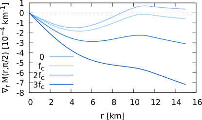
Figure 7: (Color online) Gradient of the magnetic potential at the equator as a function of the radial coordinate for different values of the rotation frequency, and for the $L=55$ MeV model, and a $M_{b}=1.5\mathrm{M}_{\odot}$ star with $B_{s}\approx 2.2\times 10^{16}$ G.

As already discussed in Franzon et al. (2016b) and shown in the last section, the magnetic potential function, $M$, may present a concave shape and, thus, a local minimum. Since the Lorentz force is proportional to the gradient of $M$, this minimum, at the equator, corresponds to a line of points where the Lorentz force changes sign, and defines the neutral line. This means that there is a region in which the magnetic field acts towards the center of the star, and another one where the Lorentz force pushes outwards. A change of the direction of the Lorentz force, if occurring in a fragile region as the crust, could be associated to the breaking of the stellar crust and leading to flares. As discussed in the previous section, in Lander and Jones (2011) it was argued that in the neighborhood of the neutral line large instabilities could develop in a star with a poloidal field.

Taking into account the effects of rotation, for each model and mass, there is a frequency (hereafter referred to as critical frequency, and designated by $f_{crit}$) at which the Lorentz force sign changes. This effect is shown in Figure 7, where we present the radial component of $\nabla M$, measured along the equatorial plane with $\theta=\frac{\pi}{2}$. It is seen that for a frequency $f\gtrsim f_{crit}$, the Lorentz force is always pointing outwards. The larger the frequency, the stronger the Lorentz force.

In Table 2 we present the values of the critical frequency, $f_{crit}$, for the two models considered, and for stars with $M_{b}=1.2\mathrm{M}_{\odot}$, $M_{b}=1.5\mathrm{M}_{\odot}$ and $M_{b}=1.8\mathrm{M}_{\odot}$. We note that this so called critical frequency does not depend a lot on the model considered, but only on the baryonic mass of the star, and on the magnitude of the magnetic field. The critical frequencies obtained are all above 90 Hz. As shown, for instance, in Ref. Ho et al. (2014), pulsars with strong magnetic fields have periods of the order of 1 or larger. This means that the poloidal field inside these pulsars will always have a neutral magnetic line and closed lines.

Table 2: Frequency, $f_{crit}$, at which the neutral line disappears for the two models considered, and stars with different baryonic masses. The surface magnetic field is set to $B_{s}\approx 2.2\times 10^{16}$ G.

$L$ (MeV)	Mb $(\mathrm{M}_{\odot})$	$f_{crit}$ (Hz)
55	1.2	127
	1.5	109
	1.8	96
88	1.2	125
	1.5	108
	1.8	96

In Table 3 we show how the neutral line position is altered by the inclusion of rotation for the models and masses previously considered. Similarly to what happens to the full coordinate radius of the star, the distance of the neutral line to the star centre increases with the frequency. The lower mass stars are the ones where this effect is more evident. On the other hand, for $f=50$Hz the increase is roughly the same for the two models: $\sim 2.2\%$ for the lower mass stars.

Table 3: The position of the inner crust boundaries $R_{1}$ and $R_{2}$, the NS radius $R$, and the neutral line $R_{n}$ measured along the equatorial plane, for different rotation frequencies, and stars with masses 1.2, 1.4 and 1.8 $M_{\odot}$, and described by models with $L=55$ and $L=88$ MeV. The surface magnetic field at the pole is $B_{s}\approx 2.2\times 10^{16}$ G.

$L$ (MeV)	Mb $(\mathrm{M}_{\odot})$	$R_{1}$ (km)	$R_{2}$ (km)	$R$ (km)	$R_{n}$ (km)
$f=0$ Hz
55	1.2	10.06	9.729	11.83	8.691
	1.5	10.17	9.907	11.62	8.658
	1.8	10.19	9.955	11.38	8.536
88	1.2	10.72	9.131	12.30	8.981
	1.5	10.74	9.444	11.99	8.842
	1.8	10.65	9.573	11.67	8.646
$f=0.1$ Hz
55	1.2	10.06	9.729	11.83	8.691
	1.5	10.17	9.907	11.62	8.658
	1.8	10.16	9.955	11.38	8.536
88	1.2	10.72	9.131	12.30	8.982
	1.5	10.73	9.443	11.99	8.842
	1.8	10.65	9.573	11.67	8.646
$f=10$ Hz
55	1.2	10.06	9.729	11.83	8.699
	1.5	10.17	9.907	11.62	8.668
	1.8	10.19	9.955	11.38	8.549
88	1.2	10.73	9.131	12.30	8.990
	1.5	10.74	9.444	11.99	8.852
	1.8	10.65	9.573	11.67	8.659
$f=50$ Hz
55	1.2	10.05	9.728	11.84	8.876
	1.5	10.18	9.914	11.63	8.917
	1.8	10.19	9.960	11.39	8.872
88	1.2	10.73	9.133	12.31	9.183
	1.5	10.74	9.446	11.995	9.113
	1.8	10.65	9.576	11.67	8.991

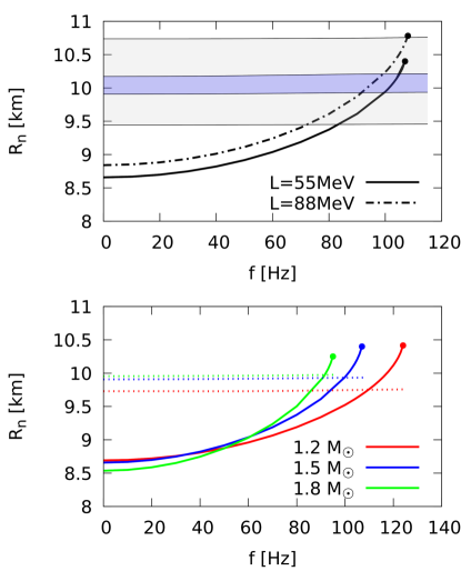
Figure 8: (Color online) Neutral line as function of the frequency. The top panel shows the results for a $1.5M_{\odot}$ star, with $L=55$ MeV (solid line, blue horizontal band) and $L=88$ MeV (dashed line, grey horizontal band). The horizontal bands correspond to the extended crust. The bottom panel shows the results for the $L=55$ MeV model, for stars with $1.2$ (red), $1.5$ (blue) and $1.8$ (green) M_⊙. The horizontal lines correspond to the crust-core boundary, i.e. $R_{2}$. In all cases, the magnetic field at the surface is set to $B_{s}\approx 2.2\times 10^{16}$ G.

As already mentioned in the previous section, stars endowed with a poloidal magnetic field may show instabilities around the neutral line, and it is believed that rotation might cease those instabilities Lander and Jones (2011). Unlike the non-rotating case, Figure 8 shows that the neutral line can indeed fall inside the crust region, when the extended crust is taken into account. In the bottom panel of the same figure, we show, for the model with $L=55$ MeV, how the neutral line is affected by the frequency increase for different masses. We conclude that lower mass stars are much more sensitive to the effects of the frequency. The results are analogous for $L=88$ MeV, however, the neutral line enters the extended crust for smaller frequencies.

IV Conclusions

In this paper, we analyse how strong magnetic fields and rotation affect the inner crust of a NS. The inner crust is complemented with an extended crust which, as reported in Fang et al. (2016, 2017a), should be taken into consideration when strong magnetic fields are present. Part of our goal was to understand how models of the same family, but with different symmetry energy slope, $L$, compare when subject to extreme magnetic fields and rotation. Our results show that the larger the slope of the symmetry energy $L$, the bigger the sensitivity of the model regarding variations of the magnetic field, which is consistent with the fact that below saturation density, the fraction of protons is smaller for larger values of $L$, and above it is larger. This is particularly evident on the difference in the size of the extended crust. The magnetic field may affect the different types of layers that exist in the crust. We verified that the Lorentz force has two local maxima, one of them localized in the region populated by pasta phases. This indicates that the geometries more susceptible to break lie in a region where some of the strongest stresses occur.

Studies on the evolution of magnetic fields in neutron stars have reported the existence of a line inside the star, the neutral line, where the magnetic field is zero. These same studies indicate the existence of instabilities around this line Lander and Jones (2011), if a pure poloidal field is considered. If a mixed magnetic field configuration is assumed, the toroidal field lies on top of the poloidal neutral line Uryu et al. (2019). We wanted to ascertain whether this line falls inside the inner crust, when one takes into account the extended crust. This was not verified for non-rotating stars, but the situation changes when one includes rotation. Given the richness of phenomena that occur at the region of the neutral line, it is expected that they will depend on the properties of matter that is present in this region. It would be interesting to understand the role that pasta phases might have in connection to known astrophysical phenomena associated with magnetars.

References

- Baym et al. (1971) G. Baym, C. Pethick, and P. Sutherland, Astrophys. J. 170, 299 (1971).
- Haensel and Pichon (1994) P. Haensel and B. Pichon, Astron. Astrophys. 283, 313 (1994).
- Rüster et al. (2006) S. B. Rüster, M. Hempel, and J. Schaffner-Bielich, Phys. Rev. C 73, 035804 (2006).
- Ravenhall et al. (1983) D. G. Ravenhall, C. J. Pethick, and J. R. Wilson, Phys. Rev. Lett. 50, 2066 (1983).
- Pais and Stone (2012) H. Pais and J. R. Stone, Phys. Rev. Lett. 109, 151101 (2012).
- Pais and Providência (2016) H. Pais and C. Providência, Phys. Rev. C 94, 015808 (2016).
- Watanabe et al. (2005) G. Watanabe, T. Maruyama, K. Sato, K. Yasuoka, and T. Ebisuzaki, Phys. Rev. Lett. 94, 031101 (2005).
- Lorimer (2008) D. R. Lorimer, Living Reviews in Relativity 11, 8 (2008).
- Lai and Shapiro (1991) D. Lai and S. L. Shapiro, Astrophys. J. 383, 745 (1991).
- Cardall et al. (2001) C. Y. Cardall, M. Prakash, and J. M. Lattimer, Astrophys. J. 554, 322 (2001).
- Steiner and Watts (2009) A. W. Steiner and A. L. Watts, Phys. Rev. Lett. 103, 181101 (2009).
- Gabler et al. (2013) M. Gabler, P. Cerda-Duran, J. A. Font, E. Muller, and N. Stergioulas, Mon. Not. Roy. Astron. Soc. 430, 1811 (2013).
- Sotani et al. (2013) H. Sotani, K. Nakazato, K. Iida, and K. Oyamatsu, Mon. Not. Roy. Astron. Soc. 434, 2060 (2013).
- Deibel et al. (2014) A. T. Deibel, A. W. Steiner, and E. F. Brown, Phys. Rev. C 90, 025802 (2014).
- Sotani et al. (2019) H. Sotani, K. Iida, and K. Oyamatsu, Mon. Not. Roy. Astron. Soc. 489, 3022 (2019).
- Lander et al. (2020) S. K. Lander, P. Haensel, B. Haskell, J. L. Zdunik, and M. Fortin, (2020), arXiv:2007.14609 [astro-ph.HE] .
- Potekhin and Chabrier (2013) A. Y. Potekhin and G. Chabrier, Astron. Astrophys. 550, A43 (2013).
- Chamel et al. (2012) N. Chamel, R. L. Pavlov, L. M. Mihailov, C. J. Velchev, Z. K. Stoyanov, Y. D. Mutafchieva, M. D. Ivanovich, J. M. Pearson, and S. Goriely, Phys. Rev. C 86, 055804 (2012).
- Chamel et al. (2015) N. Chamel, Z. K. Stoyanov, L. M. Mihailov, Y. D. Mutafchieva, R. L. Pavlov, and C. J. Velchev, Phys. Rev. C 91, 065801 (2015).
- Stein et al. (2016) M. Stein, J. Maruhn, A. Sedrakian, and P. G. Reinhard, Phys. Rev. C 94, 035802 (2016).
- Chatterjee et al. (2015) D. Chatterjee, T. Elghozi, J. Novak, and M. Oertel, Mon. Not. Roy. Astron. Soc. 447, 3785 (2015).
- Fang et al. (2016) J. Fang, H. Pais, S. Avancini, and C. Providência, Phys. Rev. C 94, 062801 (2016).
- Fang et al. (2017a) J. Fang, H. Pais, S. Pratapsi, S. Avancini, J. Li, and C. Providência, Phys. Rev. C 95, 045802 (2017a).
- Fang et al. (2017b) J. Fang, H. Pais, S. Pratapsi, and C. Providência, Phys. Rev. C 95, 062801 (2017b).
- Chen (2017) Y. J. Chen, Phys. Rev. C 95, 035807 (2017).
- Bonazzola et al. (1993) S. Bonazzola, E. Gourgoulhon, M. Salgado, and J. Marck, Astron. Astrophys. 278, 421 (1993).
- Bocquet et al. (1995) M. Bocquet, S. Bonazzola, E. Gourgoulhon, and J. Novak, Astron. Astrophys. 301, 757 (1995).
- Franzon et al. (2016a) B. Franzon, V. Dexheimer, and S. Schramm, Mon. Not. Roy. Astron. Soc. 456, 2937 (2016a).
- Franzon et al. (2016b) B. Franzon, R. O. Gomes, and S. Schramm, Mon. Not. Roy. Astron. Soc. 463, 571 (2016b).
- Markey and Tayler (1973) P. Markey and R. J. Tayler, Mon. Not. Roy. Astron. Soc. 163, 77 (1973).
- Lander and Jones (2011) S. K. Lander and D. I. Jones, Mon. Not. Roy. Astron. Soc. 412, 1730 (2011).
- Haskell et al. (2008) B. Haskell, L. Samuelsson, K. Glampedakis, and N. Andersson, Mon. Not. Roy. Astron. Soc. 385, 531 (2008).
- Lander and Jones (2009) S. K. Lander and D. I. Jones, Mon. Not. Roy. Astron. Soc. 395, 2162 (2009).
- Pili et al. (2017) A. G. Pili, N. Bucciantini, and L. Del Zanna, Mon. Not. Roy. Astron. Soc. 470, 2469 (2017).
- Uryu et al. (2019) K. Uryu et al., Phys. Rev. D 100, 123019 (2019).
- Frieben and Rezzolla (2012) J. Frieben and L. Rezzolla, Mon. Not. Roy. Astron. Soc. 427, 3406 (2012).
- Goldreich and Reisenegger (1992) P. Goldreich and A. Reisenegger, Astrophys. J. 395, 250 (1992).
- de Lima et al. (2013) R. C. R. de Lima, S. S. Avancini, and C. Providência, Phys. Rev. C 88, 035804 (2013).
- Oertel et al. (2017) M. Oertel, M. Hempel, T. Klähn, and S. Typel, Rev. Mod. Phys. 89, 015007 (2017).
- Vidaña et al. (2009) I. Vidaña, C. Providência, A. Polls, and A. Rios, Phys. Rev. C 80, 045806 (2009).
- Grill et al. (2014) F. Grill, H. Pais, C. Providência, I. Vidaña, and S. S. Avancini, Phys. Rev. C 90, 045803 (2014).
- Ducoin et al. (2008) C. Ducoin, C. Providência, A. M. Santos, L. Brito, and P. Chomaz, Phys. Rev. C 78, 055801 (2008).
- Grill et al. (2012) F. Grill, C. Providência, and S. S. Avancini, Phys. Rev. C 85, 055808 (2012).
- Franzon et al. (2017) B. Franzon, R. Negreiros, and S. Schramm, Phys. Rev. D 96, 123005 (2017).
- Schneider et al. (2014) A. S. Schneider, D. K. Berry, C. M. Briggs, M. E. Caplan, and C. J. Horowitz, Phys. Rev. C 90, 055805 (2014).
- Schneider et al. (2016) A. S. Schneider, D. K. Berry, M. E. Caplan, C. J. Horowitz, and Z. Lin, Phys. Rev. C 93, 065806 (2016).
- Caplan et al. (2018) M. E. Caplan, A. S. Schneider, and C. J. Horowitz, Phys. Rev. Lett. 121, 132701 (2018).
- Ho et al. (2014) W. C. G. Ho, H. Klus, M. J. Coe, and N. Andersson, Mon. Not. Roy. Astron. Soc. 437, 3664 (2014).