An Accurate, Scalable and Verifiable Protocol for Federated Differentially Private Averaging

Abstract

Learning from data owned by several parties, as in federated learning, raises challenges regarding the privacy guarantees provided to participants and the correctness of the computation in the presence of malicious parties. We tackle these challenges in the context of distributed averaging, an essential building block of federated learning algorithms. Our first contribution is a scalable protocol in which participants exchange correlated Gaussian noise along the edges of a graph, complemented by independent noise added by each party. We analyze the differential privacy guarantees of our protocol and the impact of the graph topology under colluding malicious parties, showing that we can nearly match the utility of the trusted curator model even when each honest party communicates with only a logarithmic number of other parties chosen at random. This is in contrast with protocols in the local model of privacy (with lower utility) or based on secure aggregation (where all pairs of users need to exchange messages). Our second contribution enables users to prove the correctness of their computations without compromising the efficiency and privacy guarantees of the protocol. Our construction relies on standard cryptographic primitives like commitment schemes and zero knowledge proofs.

1 Introduction

Individuals are producing ever growing amounts of personal data, which in turn fuel innovative services based on machine learning (ML). The classic centralized paradigm consists in collecting, storing and analyzing this data on a (supposedly trusted) central server or in the cloud, which poses well documented privacy risks for the users. With the increase of public awareness and regulations, we are witnessing a shift towards a more decentralized paradigm where personal data remains on each user’s device, as can be seen from the growing popularity of federated learning kairouz2019advances . In this setting, users typically do not trust the central server (if any), or each other, which introduces new issues regarding privacy and security. First, the information shared by users during the decentralized training protocol can reveal a lot about their private data (see Melis2019 ; Shokri2019 ; inverting for inference attacks on federated learning). Formal guarantees such as differential privacy (DP) Dwork2006a are needed to provably mitigate this and convince users to participate. Second, malicious users may send incorrect results to bias the learned model in arbitrary ways Hayes2018 ; Bhagoji2019 ; Bagdasaryan2020 . Ensuring the correctness of the computation is crucial to persuade service providers to move to a more decentralized and privacy-friendly setting.

In this work, we tackle these challenges in the context of private distributed averaging. In this canonical problem, the objective is to privately compute an estimate of the average of values owned by many users who do not want to disclose them. Beyond simple data analytics, distributed averaging is of high relevance to modern ML. Indeed, it is the key primitive used to aggregate user updates in gradient-based distributed and federated learning algorithms minibatch_local_sgd ; local_sgd ; mcmahan2016communication ; Jayaraman2018 ; cp-sgd ; kairouz2019advances . It also allows to train ML models whose sufficient statistics are averages (e.g., linear models and decision trees). Distributed averaging with differential privacy guarantees has thus attracted a lot of interest in recent years. In the strong model of local differential privacy (LDP) Kasiviswanathan2008 ; d13 ; kairouz2015secure ; Kairouz2016a ; discrete_dis_local ; trilemma_neurips20 , each user randomizes its input locally before sending it to an untrusted aggregator. Unfortunately, the best possible error for the estimated average with $n$ users is of the order $O(\sqrt{n})$ larger than in the centralized model of DP where a trusted curator aggregates data in the clear and perturbs the output Chan2012 . To fill this gap, some work has explored relaxations of LDP that make it possible to match the utility of the trusted curator model. This is achieved through the use of cryptographic primitives such as secure aggregation Dwork2006ourselves ; ChanSS12 ; Shi2011 ; Bonawitz2017a ; Jayaraman2018 and secure shuffling amp_shuffling ; Cheu2019 ; Balle2020 ; Ghazi2020ICML . Many of these solutions however assume that all users truthfully follow the protocol (they are honest-but-curious) and/or give significant power (ability to reveal sensitive data) to a small number of servers. Furthermore, their practical implementation poses important challenges when the number of parties is large: for instance, the popular secure aggregation approach of Bonawitz2017a requires all $O(n^{2})$ pairs of users to exchange messages.

In this context, our contribution is fourfold.

• First, we propose Gopa, a novel decentralized differentially private averaging protocol that relies on users exchanging (directly or through a server) some pairwise-correlated Gaussian noise terms along the edges of a graph so as to mask their private values without affecting the global average. This ultimately canceling noise is complemented by the addition of independent (non-canceling) Gaussian noise by each user.

• Second, we analyze the differential privacy guarantees of Gopa. Remarkably, we establish that our approach can achieve nearly the same privacy-utility trade-off as a trusted curator who would average the values of honest users, provided that the graph of honest-but-curious users is connected and the pairwise-correlated noise variance is large enough. In particular, for $n_{H}$ honest-but-curious users and any fixed DP guarantee, the variance of the estimated average is only $n_{H}/(n_{H}-1)$ times larger than with a trusted curator, a factor which goes to $1$ as $n_{H}$ grows. We further show that if the graph is well-connected, the pairwise-correlated noise variance can be significantly reduced.

• Third, to ensure both scalability and robustness to malicious users, we propose a randomized procedure in which each user communicates with only a logarithmic number of other users while still matching the privacy-utility trade-off of the trusted curator. Our analysis is novel and requires to leverage and adapt results from random graph theory on embedding spanning trees in random graphs. Additionally, we show our protocol is robust to a fraction of users dropping out.

• Finally, we propose a procedure to make Gopa verifiable by untrusted external parties, i.e., to enable users to prove the correctness of their computations without compromising the efficiency or the privacy guarantees of the protocol. To the best of our knowledge, we are the first to propose such a procedure. It offers a strong preventive countermeasure against various attacks such as data poisoning or protocol deviations aimed at reducing utility. Our construction relies on commitment schemes and zero knowledge proofs (ZKPs), which are very popular in auditable electronic payment systems and cryptocurrencies. These cryptographic primitives scale well both in communication and computational requirements and are perfectly suitable in our untrusted decentralized setting. We use classic ZKPs to design a procedure for the generation of noise with verifiable distribution, and ultimately to prove the correctness of the final computation (or detect malicious users who did not follow the protocol). Crucially, the privacy guarantees of the protocol are not compromised by this procedure, while the integrity of the computation relies on a standard discrete logarithm assumption. In the end, we argue that our protocol offers correctness guarantees that are essentially equivalent to the case where a trusted curator would hold the private data of users.

The paper is organized as follows. Section 2 introduces the problem setting. We discuss the related work in more details in Section 3. The Gopa protocol is introduced in Section 4 and we analyze its differential privacy guarantees in Section 5. We present our procedure to ensure correctness against malicious behavior in Section 6, and summarize computational and communication costs in Section 7. Finally, we present some experimental results in Section 8 and conclude with future lines of research in Section 9.

2 Notations and Setting

We consider a set $U=\{1,\dots,n\}$ of $n\geq 3$ users (parties). Each user $u\in U$ holds a private value $X_{u}$, which can be thought of as being computed from the private dataset of user $u$. We assume that $X_{u}$ lies in a bounded interval of $\mathbb{R}$ (without loss of generality, we assume $X_{u}\in[0,1]$). The extension to the vector case is straightforward. We denote by $X$ the column vector $X=[X_{1},\dots,X_{n}]^{\top}\in[0,1]^{n}$ of private values. Unless otherwise noted, all vectors are column vectors. Users communicate over a network represented by a connected undirected graph $G=(U,E)$, where $\{u,v\}\in E$ indicates that users $u$ and $v$ are neighbors in $G$ and can exchange secure messages. For a given user $u$, we denote by $N(u)=\{v:\{u,v\}\in E\}$ the set of its neighbors. We note that in settings where users can only communicate with a server, the latter can act as a relay that forwards (encrypted and authenticated) messages between users, as done in secure aggregation Bonawitz2017a .

The users aim to collaboratively estimate the average value $X^{avg}=\frac{1}{n}\sum_{u=1}^{n}X_{u}$ without revealing their individual private values. Such a protocol can be readily used to privately execute distributed ML algorithms that interact with data through averages over values computed locally by the participants, but do not actually need to see the individual values. We give two concrete examples below.

Example 1 (Linear regression)

Let $\lambda\geq 0$ be a public parameter. Each user $u$ holds a private feature vector $\phi_{u}=[\phi_{u}^{1},\dots,\phi_{u}^{d}]\in\mathbb{R}^{d}$ and a private label $y_{u}\in\mathbb{R}$. The goal is to solve a ridge regression task, i.e. find $\theta^{*}\in\operatorname*{arg\,min}_{\theta}\frac{1}{n}\sum_{u\in U}(\phi_{u}^{\top}\theta-y_{u})^{2}+\lambda\|\theta\|^{2}$. $\theta^{*}$ can be computed in closed form from the quantities $\frac{1}{n}\sum_{u\in U}\phi_{u}^{i}y_{u}$ and $\frac{1}{n}\sum_{u\in U}\phi_{u}^{i}\phi_{u}^{j}$ for all $i,j\in\{1,\dots,d\}$.

Example 2 (Federated ML)

In federated learning kairouz2019advances and distributed empirical risk minimization, each user $u$ holds a private dataset $\mathcal{D}_{u}$ and the goal is to find $\theta^{*}$ such that $\theta^{*}\in\operatorname*{arg\,min}_{\theta}\frac{1}{n}\sum_{u\in U}f(\theta;\mathcal{D}_{u})$ where $f$ is some loss function. Popular algorithms minibatch_local_sgd ; local_sgd ; mcmahan2016communication ; Jayaraman2018 ; cp-sgd all follow the same high-level procedure: at round $t$, each user $u$ computes a local update $\theta_{u}^{t}$ based on $\mathcal{D}_{u}$ and the current global model $\theta^{t-1}$, and the updated global model is computed as $\theta^{t}=\frac{1}{n}\sum_{u}\theta_{u}^{t}$.

Threat model. We consider two commonly adopted adversary models formalized by goldreich1998secure and used in the design of many secure protocols. A honest-but-curious (honest for short) user will follow the protocol specification, but may use all the information obtained during the execution to infer information about other users. A honest user may accidentally drop out at any point of the execution (in a way that is independent of the private values $X$). On the other hand, a malicious user may deviate from the protocol execution (e.g, sending incorrect values or dropping out on purpose). Malicious users can collude, and thus will be seen as a single malicious party (the adversary) who has access to all information collected by malicious users. Our privacy guarantees will hold under the assumption that honest users communicate through secure channels, while the correctness of our protocol will be guaranteed under some form of the Discrete Logarithm Assumption (DLA), a standard assumption in cryptography.

For a given execution of the protocol, we denote by $U^{O}$ the set of the users who remained online until the end (i.e., did not drop out). Users in $U^{O}$ are either honest or malicious: we denote by $U^{H}\subseteq U^{O}$ those who are honest, by $n_{H}=|U^{H}|$ their number and by $\rho=n_{H}/n$ their proportion with respect to the total number of users. We also denote by $G^{H}=(U^{H},E^{H})$ the subgraph of $G$ induced by the set of honest users $U^{H}$, i.e., $E^{H}=\{\{u,v\}\in E:u,v\in U^{H}\}$. The properties of $G$ and $G^{H}$ will play a key role in the privacy and scalability guarantees of our protocol.

Privacy definition. Our goal is to design a protocol that satisfies differential privacy (DP) Dwork2006a , which has become a gold standard in private information release.

Definition 1 (Differential privacy)

Let $\varepsilon>0,\delta\geq 0$. A (randomized) protocol $\mathcal{A}$ is $(\varepsilon,\delta)$-differentially private if for all neighboring datasets $X=[X_{1},\dots,X_{n}]$ and $X^{\prime}=[X^{\prime}_{1},\dots,X_{n}]$ differing only in a single data point, and for all sets of possible outputs $\mathcal{O}$, we have:

$$\Pr(\mathcal{A}(X)\in\mathcal{O})\leq e^{\varepsilon}\Pr(\mathcal{A}(X^{\prime})\in\mathcal{O})+\delta.$$ (1)

3 Related Work

Approach	Com. per party	MSE	Verif	Risks
Central DP Dwork2014a	$O(1)$	$O(1/n^{2})$	No	Trusted curator
Local DP Kasiviswanathan2008	$O(1)$	$O(1/n)$	No
Verifiable secret sharing Dwork2006ourselves	$O(n)$	$O(1/n^{2})$	Yes
Secure agg. Bonawitz2017a + DP pmlr-v139-kairouz21a ; skellam	$O(n)$	$O(1/n^{2})$	No	Honest users
CAPE imtiaz2021distributed	$O(n)$	$O(1/n^{2})$	No
Shuffling Balle2020	$O(1+\log(1/\delta))$	$O(1/n^{2})$	No	Trusted shuffler
GOPA (this work)	$O(\log n)$	$O(1/n^{2})$	Yes

Table 1: Comparison of GOPA with previous DP averaging approaches with their communication cost per party, mean squared error (MSE), verifiability (Verif) and additional risks.

In this section we review the most important work related to ours. A set of key approaches together with their main features are summarized in Table 1.

Distributed averaging is a key subroutine in distributed and federated learning minibatch_local_sgd ; local_sgd ; mcmahan2016communication ; Jayaraman2018 ; cp-sgd ; kairouz2019advances . Therefore, any improvement in the privacy-utility-communication trade-off for averaging implies gains for many ML approaches downstream.

Local differential privacy (LDP) Kasiviswanathan2008 ; d13 ; kairouz2015secure ; Kairouz2016a ; discrete_dis_local requires users to locally randomize their input before they send it to an untrusted aggregator. This very strong model of privacy comes at a significant cost in utility: the best possible mean squared is of order $1/n^{2}$ in the trusted curator model while it is of order $1/n$ in LDP Chan2012 ; trilemma_neurips20 . This limits the usefulness of the local model to industrial settings where the number of participants is huge rappor15 ; telemetry17 . Our approach belongs to the recent line of work which attempts to relax the LDP model so as to improve utility without relying on a trusted curator (or similarly on a small fixed set of parties).

Previous work considered the use of cryptographic primitives like secure aggregation protocols, which can be used to compute the (exact) average of private values Dwork2006ourselves ; Shi2011 ; Bonawitz2017a ; ChanSS12 . While secure aggregation allows in principle to recover the utility of the trusted curator model, it suffers three main drawbacks. Firstly, existing protocols require $\Omega(n)$ communication per party, which is hardly feasible beyond a few hundred or thousand users. In contrast, we propose a protocol which requires only $O(\log n)$ communication. Secondly, combining secure aggregation with DP is nontrivial as the noise must be added in a distributed fashion and in the discrete domain. Existing complete systems pmlr-v139-kairouz21a ; skellam assume an ideal secure aggregation functionality which does not reflect the impact of colluding/malicious users. In these more challenging settings, it is not clear how to add the necessary noise for DP and what the resulting privacy/utility trade-offs would be. Alternatively, Jayaraman2018 adds the noise within the secure protocol but relies on two non-colluding servers. Thirdly, most of the above schemes are not verifiable. One exception is the verifiable secret sharing approach of Dwork2006ourselves , which again induces $\Omega(n)$ communication. Finally, we note that secure aggregation typically uses uniformly distributed pairwise masks, hence a single residual term completely destroys the utility. In contrast, we use Gaussian pairwise masks that have zero mean and bounded variance, which provides more robustness but requires the more involved privacy analysis we present in Section 5.

Recently, the shuffle model of privacy Cheu2019 ; amp_shuffling ; Hartmann2019 ; Balle2020 ; Ghazi2020ICML , where inputs are passed to a trusted/secure shuffler that obfuscates the source of the messages, has been studied theoretically as an intermediate point between the local and trusted curator models. For differentially private averaging, the shuffle model allows to match the utility of the trusted curator setting Balle2020 . However, practical implementations of secure shuffling are not discussed in these works. Existing solutions typically rely on multiple layers of routing servers Dingledine2004 with high communication overhead and non-collusion assumptions. Anonymous communication is also potentially at odds with the identification of malicious parties. To the best of our knowledge, all protocols for averaging in the shuffle model assume honest-but-curious parties.

The protocol proposed in imtiaz2021distributed uses correlated Gaussian noise to achieve trusted curator utility for averaging, but the dependence structure of the noise must be only at the global level (i.e., noise terms sum to zero over all users). Generating such noise actually requires a call to a secure aggregation primitive, which incurs $\Omega(n)$ communication per party as discussed above. In contrast, our pairwise-canceling noise terms can be generated with only $O(\log n)$ communication. Furthermore, imtiaz2021distributed assume honest parties, while our protocol is robust to malicious participants.

In summary, an original aspect of our work is to match the privacy-utility trade-off of the trusted curator model at a relatively low cost without requiring to trust a fixed small set of parties. By spreading trust over sufficiently many parties, we ensure that even in the unlikely case where many parties collude they will not be able to infer much sensitive information, reducing the incentive to collude. We are not aware of other differential privacy work sharing this feature. Overall, our protocol provides a unique combination of three important properties: (a) utility of same order as trusted curator setting, (b) logarithmic communication per user, and (c) robustness to malicious users.

4 Proposed Protocol

In this section we describe our protocol called Gopa (GOssip noise for Private Averaging). The high-level idea of Gopa is to have each user $u$ mask its private value by adding two different types of noise. The first type is a sum of pairwise-correlated noise terms $\Delta_{u,v}$ over the set of neighbors $v\in N(u)$ such that each $\Delta_{u,v}$ cancels out with the $\Delta_{v,u}$ of user $v$ in the final result. The second type of noise is an independent term $\eta_{u}$ which does not cancel out. At the end of the protocol, each user has generated a noisy version $\hat{X}_{u}$ of its private value $X_{u}$, which takes the following form:

$$\hat{X}_{u}=X_{u}+\textstyle\sum_{v\in N(u)}\Delta_{u,v}+\eta_{u}.$$ (2)

Algorithm 1 presents the detailed steps. Neighboring nodes $\{u,v\}\in E$ contact each other to draw a real number from the Gaussian distribution $\mathcal{N}(0,\sigma_{\Delta}^{2})$, that $u$ adds to its private value and $v$ subtracts. Intuitively, each user thereby distributes noise masking its private value across its neighbors so that even if some of them are malicious and collude, the remaining noise values will be enough to provide the desired privacy guarantees. The idea is reminiscent of uniformly random pairwise masks in secure aggregation Bonawitz2017a but we use Gaussian noise and restrict exchanges to the edges of the graph instead of requiring messages between all pairs of users. As in gossip algorithms random_gossip , the pairwise exchanges can be performed asynchronously and in parallel. Additionally, every user $u\in U$ adds an independent noise term $\eta_{u}\sim\mathcal{N}{(0,\sigma_{\eta}^{2})}$ to its private value. This noise will ensure that the final estimate of the average satisfies differential privacy (see Section 5). The pairwise and independent noise variances $\sigma_{\Delta}^{2}$ and $\sigma_{\eta}^{2}$ are public parameters of the protocol.

Algorithm 1 Gopa protocol

Input: $G=(U,E)$, $(X_{u})_{u\in U}$, $\sigma_{\Delta}^{2},\sigma_{\eta}^{2}\in\mathbb{R}^{+}$

1:  for all neighbor pairs $\{u,v\}\in E$ s.t. $u<v$ do

2:     $u$ and $v$ draw a random $y\sim\mathcal{N}(0,\sigma_{\Delta}^{2})$ and set $\Delta_{u,v}\leftarrow y$, $\Delta_{v,u}\leftarrow-y$

3:  end for

4:  for all users $u\in U$ do

5:     $u$ draws a random $\eta_{u}\sim\mathcal{N}(0,\sigma_{\eta}^{2})$ and reveals noisy value $\hat{X}_{u}\leftarrow X_{u}+\sum_{v\in N(u)}\Delta_{u,v}+\eta_{u}$

6:  end for

Utility of Gopa. The protocol generates a set of noisy values $\hat{X}=[\hat{X}_{1},\dots,\hat{X}_{n}]^{\top}$ which are then publicly released. They can be sent to an untrusted aggregator, or averaged in a decentralized way via gossiping random_gossip . In any case, the estimated average is given by $\hat{X}^{avg}=\frac{1}{n}\sum_{u\in U}\hat{X}_{u}=X^{avg}+\frac{1}{n}\sum_{u\in U}\eta_{u},$ which has expected value $X^{avg}$ and variance $\sigma_{\eta}^{2}/n$. Recall that the local model of DP, where each user releases a locally perturbed input without communicating with other users, would require $\sigma_{\eta}^{2}=O(1)$. In contrast, we would like the total amount of independent noise to be of order $O(1/n_{H})$ as needed to protect the average of honest users with the standard Gaussian mechanism in the trusted curator model of DP Dwork2014a . We will show in Section 5 that we can achieve this privacy-utility trade-off by choosing an appropriate variance $\sigma_{\Delta}^{2}$ for our pairwise noise terms.

Dealing with dropout. A user $u\notin U^{O}$ who drops out during the execution of the protocol does not actually publish any noisy value (i.e., $\hat{X}_{u}$ is empty). The estimated average is thus computed by averaging only over the noisy values of users in $U^{O}$. Additionally, any residual noise term that a user $u\notin U^{O}$ may have exchanged with a user $v\in U^{O}$ before dropping out can be “rolled back” by having $v$ reveal $\Delta_{u,v}$ so it can be subtracted from the result (we will ensure this does not threaten privacy by having sufficiently many neighbors, see Section 5.4). We can thus obtain an estimate of $\frac{1}{|U^{O}|}\sum_{u\in U^{O}}X_{u}$ with variance $\sigma_{\eta}^{2}/|U^{O}|$. Note that even if some residual noise terms are not rolled back, e.g. to avoid extra communication, the estimate remains unbiased (with a larger variance that depends on $\sigma_{\Delta}^{2}$). This is a rather unique feature of Gopa which comes from the use of Gaussian noise rather than the uniformly random noise used in secure aggregation Bonawitz2017a . We discuss strategies to handle users dropping out in more details in Appendix B.2.

5 Privacy Guarantees

Our goal is to prove differential privacy guarantees for Gopa. First, we develop in Section 5.1 a general result providing privacy guarantees as a function of the structure of the communication graph $G^{H}$, i.e., the subgraph of $G$ induced by $U^{H}$. Then, in Sections 5.2 and 5.3, we study the special cases of the path graph and the complete graph respectively, showing they are the worst and best cases in terms of privacy. Yet, we show that as long as $G^{H}$ is connected and the variance $\sigma_{\Delta}^{2}$ for the pairwise (canceling) noise is large enough Gopa can (nearly) match the privacy-utility trade-off of the trusted curator setting. In Section 5.4, we propose a randomized procedure to construct the graph $G$ and show that it strikes a good balance between privacy and communication costs. In each section, we first discuss the result and its consequences, and then present the proof. In Section 5.5, we summarize our results and provide further discussion.

5.1 Effect of the Communication Structure on Privacy

The strength of the privacy guarantee we can prove depends on the communication graph $G^{H}$ over honest users. Intuitively, this is because the more terms $\Delta_{u,v}$ a given honest user $u$ exchanges with other honest users $v$, the more he/she spreads his/her secret over others and the more difficult it becomes to estimate the private value $X_{u}$. We first introduce in Section 5.1.1 a number of preliminary concepts. Next, in Section 5.1.2, we prove an abstract result, Theorem 5.1, which gives DP guarantees for Gopa that depend on the choice of a labeling $t$ of the graph $G^{H}$.

In Section 5.1.3 we discuss a number of implications of Theorem 5.1 which provide some insight into the dependency between the structure of $G^{H}$ and the privacy of Gopa, and will turn out helpful in the proofs of Theorems 5.2, 5.3 and 5.4.

5.1.1 Preliminary Concepts

Recall that each user $u\in U^{O}$ who does not drop out generates $\hat{X}_{u}$ from its private value $X_{u}$ by adding pairwise noise terms $\bar{\Delta}_{u}=\sum_{v\in N(u)}\Delta_{u,v}$ (with $\Delta_{u,v}+\Delta_{v,u}=0$) as well as independent noise $\eta_{u}$. All random variables $\Delta_{u,v}$ (with $u<v$) and $\eta_{u}$ are independent. We thus have the system of linear equations

$${\hat{X}}=X+\bar{\Delta}+\eta,$$

where $\bar{\Delta}=(\bar{\Delta}_{u})_{u\in U^{O}}$ and $\eta=(\eta_{u})_{u\in U^{O}}$.

We now define the knowledge acquired by the adversary (colluding malicious users) during a given execution of the protocol. It consists of the following:

1. the noisy value $\hat{X}_{u}$ of all users $u\in U^{O}$ who did not drop out,

2. the private value $X_{u}$ and the noise $\eta_{u}$ of the malicious users, and

3. all $\Delta_{u,v}$’s for which $u$ or $v$ is malicious.

We also assume that the adversary knows the full network graph $G$ and all the pairwise noise terms exchanged by dropped out users (since they can be rolled back, as explained in Section 4). The only unknowns are thus the private value $X_{u}$ and independent noise $\eta_{u}$ of each honest user $u\in U^{H}$, as well as the $\Delta_{u,v}$ values exchanged between pairs of honest users $\{u,v\}\in E^{H}$.

Letting $N^{H}(u)=\{v:\{u,v\}\in E^{H}\}$, from the above knowledge the adversary can subtract $\sum_{v\in N(u)\setminus N^{H}(u)}\Delta_{u,v}$ from $\hat{X}_{u}$ to obtain

$$\hat{X}_{u}^{H}=X_{u}+\sum_{u\in N^{H}(u)}\Delta_{u,v}+\eta_{u}$$

for every honest $u\in U^{H}$. The view of the adversary can thus be summarized by the vector $\hat{X}^{H}=(\hat{X}^{H}_{u})_{u\in U^{H}}$ and the correlation between its elements. Let ${\hat{X}}^{H}_{u}={\hat{X}}_{u}-\sum_{v\in N(u)\setminus N^{H}(u)}\Delta_{u,v}$. Let $X^{H}=(X_{u})_{u\in U^{H}}$ be the vector of private values restricted to the honest users and similarly $\eta^{H}=(\eta_{u})_{u\in U^{H}}$. Let the directed graph $(U^{H},{{\vec{E}}^{H}})$ be an arbitrary orientation of the undirected graph $G^{H}=(U^{H},E^{H})$, i.e., for every edge $\{u,v\}\in E^{H}$, the set ${{\vec{E}}^{H}}$ either contains the arc $(u,v)$ or the arc $(v,u)$. For every arc $(u,v)\in{{\vec{E}}^{H}}$, let $\Delta_{(u,v)}=\Delta_{u,v}=-\Delta_{v,u}$. Let $\Delta^{H}=(\Delta_{e}^{H})_{e\in{{\vec{E}}^{H}}}$ be a vector of pairwise noise values indexed by arcs from ${{\vec{E}}^{H}}$. Let $K\in\mathbb{R}^{U^{H}\times{{\vec{E}}^{H}}}$ denote the oriented incidence matrix of the graph $G^{H}$, i.e., for $(u,v)\in{{\vec{E}}^{H}}$ and $w\in U^{H}\setminus\{u,v\}$ there holds $K_{u,(u,v)}=-1$, $K_{v,(u,v)}=1$ and $K_{w,(u,v)}=0$. In this way, we can rewrite the system of linear equations as

$${\hat{X}}^{H}=X^{H}+K\Delta^{H}+\eta^{H}.$$ (3)

Now, adapting differential privacy (Definition 1) to our setting, for any input $X$ and any possible outcome $\hat{X}$, we need to compare the probability of the outcome being equal to $\hat{X}$ when a (non-malicious) user $v_{1}\in U$ participates in the computation with private value $X_{v_{1}}^{A}$ to the probability of obtaining the same outcome when the value of $v_{1}$ is exchanged with an arbitrary value $X_{v_{1}}^{B}\in[0,1]$. Since honest users drop out independently of $X$ and do not reveal anything about their private value when they drop out, in our analysis we will fix an execution of the protocol where some set $U^{H}$ of $n_{H}$ honest users have remained online until the end of the protocol. For notational simplicity, we denote by $X^{A}$ the vector of private values $(X_{u})_{u\in U^{H}}$ of these honest users in which a user $v_{1}$ has value $X_{v_{1}}^{A}$, and by $X^{B}$ the vector where $v_{1}$ has value $X_{v_{1}}^{B}$. $X^{A}$ and $X^{B}$ differ in only in the $v_{1}$-th coordinate, and their maximum difference is $1$.

All noise variables are zero mean, so the expectation and covariance matrix of $\hat{X}^{H}$ are respectively given by:

$$\mathbb{E}\left[{\hat{X}}^{H}\right]=X^{H},\quad\hbox{var}\left({\hat{X}}^{H}\right)=\sigma_{\eta}^{2}I_{U^{H}}+\sigma_{\Delta}^{2}L,$$

where $I_{U^{H}}\in\mathbb{R}^{n_{H}\times n_{H}}$ is the identity matrix and $L=KK^{\top}$ is the graph Laplacian matrix of $G^{H}$.

Now consider the real vector space $Z=\mathbb{R}^{n_{H}}\times\mathbb{R}^{|E^{H}|}$ of all possible values pairs $(\eta^{H},\Delta^{H})$ of noise vectors of honest users. For the sake of readability, in the remainder of this section we will often drop the superscript $H$ and write $(\eta,\Delta)$ when it is clear from the context that we work in the space $Z$.

Let

$${\Sigma^{(g)}}=\left[\begin{array}[]{cc}\sigma_{\eta}^{2}I_{U^{H}}&0\\ 0&\sigma_{\Delta}^{2}I_{E^{H}}\end{array}\right],$$

and let $\Sigma^{(-g)}=\left({\Sigma^{(g)}}\right)^{-1}$, we then have a joint probability distribution of independent Gaussians:

$$P((\eta,\Delta))=C_{1}\exp\left(-\frac{1}{2}(\eta,\Delta)^{\top}\Sigma^{(-g)}(\eta,\Delta)\right),$$

where $C_{1}=(2\pi)^{-(n_{H}+|E^{H}|)/2}|{\Sigma^{(g)}}|^{-1/2}$.

Consider the following subspaces of $Z$:

$$Z^{A} = \{(\eta,\Delta)\in Z\mid\eta+K\Delta={\hat{X}}^{H}-X^{A}\},$$

$$Z^{B} = \{(\eta,\Delta)\in Z\mid\eta+K\Delta={\hat{X}}^{H}-X^{B}\}.$$

Assume that the (only) vertex for which $X^{A}$ and $X^{B}$ differ is $v_{1}$. Recall that without loss of generality, private values are in the interval $[0,1]$. Hence, if we set $X^{A}_{v_{1}}-X^{B}_{v_{1}}=1$ then $X^{A}$ and $X^{B}$ are maximally apart and also the difference between $P({\hat{X}}\mid X^{A})$ and $P({\hat{X}}|X^{B})$ will be maximal.

Now choose any vector $t=(t_{\eta},t_{\Delta})\in Z$ with $t_{\eta}=(t_{u})_{u\in U^{H}}$ and $t_{\Delta}=(t_{e})_{e\in E^{H}}$ such that $t_{\eta}+Kt_{\Delta}=X^{A}-X^{B}$. It follows that $Z^{B}=Z^{A}+t$, i.e., $Y\in Z^{A}$ if and only if $Y+t\in Z^{B}$. This only imposes one linear constraint on the vector $t$: later we will choose $t$ more precisely in a way which is most convenient to prove our privacy claims. In particular, for any $\hat{X}^{H}$ we have that $X^{A}+\eta+K\Delta=\hat{X}^{H}$ if and only if $X^{B}+(\eta+t_{\eta})+K(\Delta+t_{\Delta})=\hat{X}^{H}$. The key idea is that appropriately choosing $t$ allows us to map any noise $(\eta,\Delta)$ which results in observing ${\hat{X}}^{H}$ given dataset $X^{A}$ on a similarly likely noise $(\eta+t_{\eta},\Delta+t_{\Delta})$ which results in observing ${\hat{X}}^{H}$ given the adjacent dataset $X^{B}$.

We illustrate the meaning of $t$ using the example of Figure 1. Consider the graph $G^{H}$ of honest users shown in Figure 1(a) and databases $X^{A}$ and $X^{B}$ as defined above. The difference of neighboring databases $X^{A}-X^{B}$ is shown in Figure 1(b). Figure 1(c) illustrates a possible assignment of $t$, where $t_{\eta}=(\frac{1}{9},\dots,\frac{1}{9})$ and $t_{\Delta}=(\frac{5}{9},\frac{3}{9},\frac{3}{9},\frac{1}{9},\dots,\frac{1}{9},0,0)$.

One can see that $t=(t_{\eta},t_{\Delta})$ can be interpreted as a flow on $G^{H}$ where $t_{\Delta}$ represents the values flowing through edges, and $t_{\eta}$ represents the extent to which vertices are sources or sinks. The requirement $t_{\eta}+Kt_{\Delta}=X^{A}-X^{B}$ means that for a given user $u$ we have $\sum_{(v,u)\in{{\vec{E}}^{H}}}t_{(v,u)}-\sum_{(u,v)\in{{\vec{E}}^{H}}}t_{(u,v)}=X^{A}_{u}-X^{B}_{u}-t_{u}$, which can be interpreted as the property of a flow, i.e., the value of incoming edges minus the value of outgoing edges equals the extent to which the vertex is a source or sink (here $-t_{u}$ except for $v_{1}$ where it is $1-t_{v_{1}}$). We will use this flow $t$ to first distribute $X^{A}-X^{B}$ as equally as possible over all users, and secondly to avoid huge flows through edges. For example, in Figure 1(c), we choose $t_{\eta}$ in such a way that the difference $X^{A}_{v_{1}}-X^{B}_{v_{1}}=1$ is spread over a difference of $1/9$ at each node, and $t_{\Delta}$ is chosen to let a value $1/9$ flow from each of the vertices in $U^{H}\setminus\{v_{1}\}$ to $v_{1}$, making the flow consistent.

In the following we will first prove generic privacy guarantees for any (fixed) $t$, which will be used to map elements of $Z^{A}$ and $Z^{B}$ and bound the overall probability differences of outcomes of adjacent datasets. Next, we will instantiate $t$ for different graphs $G^{H}$ and obtain concrete guarantees.

(a) Graph $G^{H}$

(b) $X^{A}-X^{B}$

(c) Labeling $t$

Figure 1: An example of valid $t$ over a communication graph of honest users $G^{H}$. The graph $G^{H}$ is shown in Figure 1(a), the difference of neighboring databases $X^{A}-X^{B}$ in Figure 1(b), and a possible value of $t$ which evenly distributes the flow of information in Figure 1(c).

5.1.2 Abstract Differential Privacy Result

We start by proving differential privacy guarantees which depend on the particular choice of labeling $t$. Theorem 5.1 holds for all possible choices of $t$, but some choices will lead to more advantageous results than others. Later, we will apply this theorem for specific choices of $t$ for proving theorems giving privacy guarantees for communication graphs $G^{H}$ with specific properties.

We first define the function ${\Theta_{max}}:\mathbb{R}_{+}\times(0,1)\mapsto\mathbb{R}_{+}$ such that ${\Theta_{max}}$ maps pairs $(\varepsilon,\delta)$ on the largest positive value of $\theta$ satisfying

$$\varepsilon \geq\theta^{1/2}+\theta/2,$$ (4)

$$\frac{\left(\varepsilon-\theta/2\right)^{2}}{\theta} \geq 2\log\left(\frac{2}{\delta\sqrt{2\pi}}\right).$$ (5)

Note that for any $\varepsilon$ and $\delta$, any $\theta\in(0,{\Theta_{max}}]$ satisfies Eqs (4) and (5).

Theorem 5.1

Let $\varepsilon,\delta\in(0,1)$. Choose a vector $t=(t_{\eta},t_{\Delta})\in Z$ with $t_{\eta}=(t_{u})_{u\in U^{H}}$ and $t_{\Delta}=(t_{e})_{e\in E^{H}}$ such that $t_{\eta}+Kt_{\Delta}=X^{A}-X^{B}$ and let $\theta=t^{\top}\Sigma^{(-g)}t$. Under the setting introduced above, if $\theta\leq{\Theta_{max}}(\varepsilon,\delta)$ then Gopa is $(\varepsilon,\delta)$-DP, i.e.,

$$P({\hat{X}}\mid X^{A})\leq e^{\varepsilon}P({\hat{X}}\mid X^{B})+\delta.$$

The proof of this theorem is in Appendix A.1. Essentially, we adapt ideas from the privacy proof of the Gaussian mechanism Dwork2014a to our setting.

5.1.3 Discussion

Essentially, given some $\varepsilon$, Equation (4) provides a lower bound for the noise (the diagonal of ${\Sigma^{(g)}}$) to be added. Equation (4) also implies that the left hand side of Equation (5) is larger than $1$. Equation (5) may then require the noise or $\varepsilon$ to be even higher if $2\log(2/\delta\sqrt{2\pi})\geq 1$, i.e., $\delta\leq 0.48394$.

If $\delta$ is fixed, both (4) and (5) allow for smaller $\varepsilon$ if $\theta$ is smaller. Let us analyze the implications of this result. We know that $\theta=\sigma_{\eta}^{-2}t_{\eta}^{\top}t_{\eta}+\sigma_{\Delta}^{-2}t_{\Delta}^{\top}t_{\Delta}$. As we can make $\sigma_{\Delta}$ arbitrarily large without affecting the variance of the output of the algorithm (the pairwise noise terms canceling each other) and thus make the second term $\sigma_{\Delta}^{-2}t_{\Delta}^{\top}t_{\Delta}$ arbitrarily small, our first priority to achieve a strong privacy guarantee will be to chose a $t$ making $\sigma_{\eta}^{-2}t_{\eta}^{\top}t_{\eta}$ small. We have the following lemma.

Lemma 1

In the setting described above, for any $t$ chosen as in Theorem 5.1 we have:

$$\sum_{u\in U^{H}}t_{u}=1.$$ (6)

Therefore, the vector $t_{\eta}$ satisfying Equation (6) and minimizing $t_{\eta}^{\top}t_{\eta}$ is the vector $\mathbbm{1}_{n_{H}}/n_{H}$, i.e., the vector containing $n_{H}$ components with value $1/n_{H}$. The proofs of the several specializations of Theorem 5.1 we will present will all be based on this choice for $t_{\eta}$. The proof of Lemma 1 can be found in Appendix A.2, along with the proof of another constraint that we derive from these observations.

Lemma 2

In the setting described above with $t$ as defined in Theorem 5.1, if $t_{\eta}=\mathbbm{1}_{n_{H}}/n_{H}$, then $G^{H}$ must be connected.

Given a fixed privacy level and fixed variance of the output, a second priority is to minimize $\sigma_{\Delta}$, as this may be useful when a user drops out and the noise he/she exchanged cannot be rolled back or would take too much time to roll back (see Appendix B.2). For this, having more edges in $G^{H}$ implies that the vector $t_{\Delta}$ has more components and therefore typically allows a solution to $t_{\eta}+Kt_{\Delta}=X^{A}-X^{B}$ with a smaller $t_{\Delta}^{\top}t_{\Delta}$ and hence a smaller $\sigma_{\Delta}$.

5.2 Worst Case Topology

We now specialize Theorem 5.1 to obtain a worst-case result.

Theorem 5.2 (Privacy guarantee for worst-case graph)

Let $X^{A}$ and $X^{B}$ be two databases (i.e., graphs with private values at the vertices) which differ only in the value of one user. Let $\varepsilon,\delta\in(0,1)$ and ${\theta_{\hbox{{p}}}}=\frac{1}{\sigma_{\eta}^{2}n_{H}}+\frac{n_{H}}{3\sigma_{\Delta}^{2}}$. If $G^{H}$ is connected and ${\theta_{\hbox{{p}}}}\leq{\Theta_{max}}(\varepsilon,\delta)$, then Gopa is $(\varepsilon,\delta)$-differentially private, i.e., ${P({\hat{X}}\mid X^{A})}\leq e^{\varepsilon}P({\hat{X}}\mid X^{B})+\delta$.

Crucially, Theorem 5.2 holds as soon as the subgraph $G^{H}$ of honest users who did not drop out is connected. Note that if $G^{H}$ is not connected, we can still obtain a similar but weaker result for each connected component separately ($n_{H}$ is replaced by the size of the connected component).

In order to get a constant $\varepsilon$, inspecting the term ${\theta_{\hbox{{p}}}}$ shows that the variance $\sigma_{\eta}^{2}$ of the independent noise must be of order $1/n_{H}$. This is in a sense optimal as it corresponds to the amount of noise required when averaging $n_{H}$ values in the trusted curator model. It also matches the amount of noise needed when using secure aggregation with differential privacy in the presence of colluding users, where honest users need to add $n/n_{H}$ more noise to compensate for collusion Shi2011 .

Further inspection of the conditions in Theorem 5.2 also shows that the variance $\sigma_{\Delta}^{2}$ of the pairwise noise must be large enough. How large it must be actually depends on the structure of the graph $G^{H}$. Theorem 5.2 describes the worst case, which is attained when every node has as few neighbors as possible while still being connected, i.e., when $G^{H}$ is a path. In this case, Theorem 5.2 shows that the variance $\sigma_{\Delta}^{2}$ needs to be of order $n_{H}$. Recall that this noise cancels out, so it does not impact the utility of the final output. It only has a minor effect on the communication cost (the representation space of reals needs to be large enough to avoid overflows with high probability), and on the variance of the final result if some residual noise terms of dropout users are not rolled back (see Section 4).

Proof (of Theorem 5.2)

Let $T$ be a spanning tree of the (connected) communication graph $G^{H}$. Let $E^{T}$ be the set of edges in $T$. Let $t\in\mathbb{R}^{n_{H}+|E^{H}|}$ be a vector such that:

• For vertices $u\in U^{H}$, $t_{u}=1/n_{H}$.

• For edges $e\in E^{H}\setminus E^{T}$, $t_{e}=0$.

• Finally, for edges $e\in E^{T}$, we choose $t_{e}$ in the unique way such that $t_{\eta}+Kt_{\Delta}=(X^{A}-X^{B})$.

In this way, $t_{\eta}+Kt_{\Delta}$ is a vector with a $1$ on the $v_{1}$ position and $0$ everywhere else. We can find a unique vector $t$ using this procedure for any communication graph $G^{H}$ and spanning tree $T$. It holds that

$$t_{\eta}^{\top}t_{\eta}=\left(\frac{\mathbbm{1}_{n_{H}}}{n_{H}}\right)^{\top}\left(\frac{\mathbbm{1}_{n_{H}}}{n_{H}}\right)=\frac{1}{n_{H}}.$$ (7)

Both Equations (4) and (5) of Theorem 5.1, require $t^{\top}\Sigma^{(-g)}t$ to be sufficiently small. We can see $t_{\Delta}^{\top}\sigma_{\Delta}^{-2}t_{\Delta}$ is maximized (thus producing the worst case) if the spanning tree $T$ is a path $\left(v_{1}\,v_{2}\ldots v_{n_{H}}\right)$, in which case $t_{\{v_{i},v_{i+1}\}}=(n_{H}-i)/n_{H}$. Therefore,

$$t_{\Delta}^{\top}t_{\Delta} \leq \sum_{i=1}^{n_{H}-1}\left(\frac{n_{H}-i}{n_{H}}\right)^{2}=\frac{n_{H}(n_{H}-1)(2n_{H}-1)/6}{n_{H}^{2}}=\frac{(n_{H}-1)(2n_{H}-1)}{6n_{H}}.$$ (8)

Combining Equations (7) and (8) we get

$$\theta=t^{\top}\Sigma^{(-g)}t\leq\sigma_{\eta}^{-2}\frac{1}{n_{H}}+\sigma_{\Delta}^{-2}\frac{n_{H}(n_{H}-1)(2n_{H}-1)/6}{n_{H}^{2}}$$

We can see that $\theta\leq{\theta_{\hbox{{p}}}}$ and hence $\theta\leq{\Theta_{max}}(\varepsilon,\delta)$ satisfies the conditions of Theorem 5.1 and Gopa is $(\varepsilon,\delta)$-differentially private. ∎

In conclusion, we see that in the worst case $\sigma_{\Delta}^{2}$ should be large (linear in $n_{H}$) to keep $\varepsilon$ small, which has no direct negative effect on the utility of the resulting ${\hat{X}}$. On the other hand, $\sigma_{\eta}^{2}$ can be small (of the order $1/n_{H}$), which means that independent of the number of participants or the way they communicate a small amount of independent noise is sufficient to achieve DP as long as $G^{H}$ is connected.

5.3 The Complete Graph

The necessary value of $\sigma_{\Delta}^{2}$ depends strongly on the network structure. This becomes clear in Theorem 5.3, which covers the case of the complete graph and shows that for a fully connected $G^{H}$, $\sigma_{\Delta}^{2}$ can be of order $O(1/n_{H})$, which is a quadratic reduction compared to the path case.

Theorem 5.3 (Privacy guarantee for complete graph)

Let $\varepsilon,\delta\in(0,1)$ and let $G^{H}$ be the complete graph. Let $\theta_{C}=\frac{1}{\sigma_{\eta}^{2}n_{H}}+\frac{1}{\sigma_{\Delta}^{2}n_{H}}$. If $\theta_{C}\leq\Theta_{max}(\varepsilon,\delta)$, then Gopa is $(\varepsilon,\delta)$-DP.

Proof

If the communication graph is fully connected, we can use the following values for the vector $t$:

• As earlier, for $v\in U^{H}$, let $t_{v}=1/n_{H}$.

• For edges $\{u,v\}$ with $v_{1}\not\in\{u,v\}$, let $t_{\{u,v\}}=0$.

• For $u\in U^{H}\setminus\{v_{1}\}$, let $t_{\{u,v_{1}\}}=1/n_{H}$.

Again, one can verify that $t_{\eta}+Kt_{\Delta}=X^{A}-X^{B}$ is a vector with a $1$ on the $v_{1}$ position and $0$ everywhere else. In this way, again $t_{\eta}^{\top}t_{\eta}=1/n_{H}$ but now $t_{\Delta}^{\top}t_{\Delta}=(n_{H}-1)/n_{H}^{2}$ is much smaller. We now get

$$\theta=t^{\top}\Sigma^{(-g)}t=\sigma_{\eta}^{-2}/n_{H}+\sigma_{\Delta}^{-2}(n_{H}-1)/n_{H}^{2}\leq\theta_{C}\leq{\Theta_{max}}(\varepsilon,\delta).$$

Hence, we can apply Theorem 5.1 and Gopa is $(\varepsilon,\delta)$-differentially private. ∎

A practical communication graph will be between the two extremes of the path and the complete graph, as shown in the next section.

5.4 Practical Random Graphs

Our results so far are not fully satisfactory from the practical perspective, when the number of users $n$ is large. Theorem 5.2 assumes that we have a procedure to generate a graph $G$ such that $G^{H}$ is guaranteed to be connected (despite dropouts and malicious users), and requires a large $\sigma_{\Delta}^{2}$ of $O(n_{H})$. Theorem 5.3 applies if we pick $G$ to be the complete graph, which ensures connectivity of $G^{H}$ and allows smaller $O(1/n_{H})$ variance but is intractable as all $n^{2}$ pairs of users need to exchange noise.

To overcome these limitations, we propose a simple randomized procedure to construct a sparse network graph $G$ such that $G^{H}$ will be well-connected with high probability, and prove a DP guarantee for the whole process (random graph generation followed by Gopa), under much less noise than the worst-case. The idea is to make each (honest) user select $k$ other users uniformly at random among all users. Then, the edge $\{u,v\}\in E$ is created if $u$ selected $v$ or $v$ selected $u$ (or both). Such graphs are known as random $k$-out or random $k$-orientable graphs Bollobas2001a ; Fenner1982a . They have very good connectivity properties Fenner1982a ; Yagan2013a and are used in creating secure communication channels in distributed sensor networks Chan2003a . Note that Gopa can be conveniently executed while constructing the random $k$-out graph. Recall that $\rho=n_{H}/n$ is the proportion of honest users. We have the following privacy guarantees (which we prove in Appendix A.3).

Theorem 5.4 (Privacy guarantee for random $k$-out graphs)

Let $\varepsilon,\delta\in(0,1)$ and let $G$ be obtained by letting all (honest) users randomly choose $k\leq n$ neighbors. Let $k$ and $\rho=n_{H}/n$ be such that $\rho n\geq 81$, $\rho k\geq 4\log(2\rho n/3\delta)$, $\rho k\geq 6\log(\rho n/3)$ and $\rho k\geq\frac{3}{2}+\frac{9}{4}\log(2e/\delta)$. Let

$$\theta_{R} =\frac{1}{n_{H}\sigma_{\eta}^{2}}+\frac{1}{\sigma_{\Delta}^{2}}\Big{(}\frac{1}{\lfloor(k-1)\rho/3\rfloor-1}+\frac{12+6\log(n_{H})}{n_{H}}\Big{)}$$

If $\theta_{R}\leq{\Theta_{max}}(\varepsilon,\delta)$ then Gopa is $(\varepsilon,3\delta)$-differentially private.

This result has a similar form as Theorems 5.2 and 5.3 but requires $k$ to be large enough (of order $\log(\rho n)/\rho$) so that $G^{H}$ is sufficiently connected despite dropouts and malicious users. Crucially, $\sigma_{\Delta}^{2}$ only needs to be of order $1/k\rho$ to match the utility of the trusted curator, and each user needs to exchange with only $2k=O(\log n)$ peers in expectation, which is much more practical than a complete graph.

Notice that up to a constant factor this result is optimal. Indeed, in general, random graphs are not connected if their average degree is smaller than logarithmic in the number of vertices. The constant factors mainly serve for making the result practical and (unlike asymptotic random graph theory) applicable to moderately small communication graphs, as we illustrate in the next section.

5.5 Scaling the Noise

Using these results, we can precisely quantify the amount of independent and pairwise noise needed to achieve a desired privacy guarantee depending on the topology, as illustrated in the corollary below.

Corollary 1

Let $\varepsilon,\delta^{\prime}\in(0,1)$, and ${\sigma_{\eta}^{2}=c^{2}/n_{H}\varepsilon^{2}}$, where $c^{2}>2\log(1.25/\delta^{\prime})$. Given some $\kappa>0$, let $\sigma_{\Delta}^{2}=\kappa\sigma_{\eta}^{2}$ if $G$ is complete, $\sigma_{\Delta}^{2}=\kappa\sigma_{\eta}^{2}n_{H}(\frac{1}{\lfloor(k-1)\rho/3\rfloor-1}+(12+6\log(n_{H}))/n_{H})$ if it is a random $k$-out graph with $k$ and $\rho$ as in Theorem 5.4, and $\sigma_{\Delta}^{2}=\kappa\sigma_{\eta}^{2}n_{H}^{2}/3$ for an arbitrary connected $G^{H}$. Then Gopa is $(\varepsilon,\delta)$-DP with $\delta\geq a(\delta^{\prime}/1.25)^{\kappa/\kappa+1}$, where $a=3.75$ for the $k$-out graph and $1.25$ otherwise.

Table 2: Value of $\sigma_{\Delta}$ needed to ensure $(\varepsilon,\delta)$-DP with trusted curator utility for $n=10000$, $\varepsilon=0.1$, $\delta^{\prime}=1/n_{H}^{2}$, $\delta=10\delta^{\prime}$ depending on the topology, as obtained from Corollary 1 or numerical simulation.

	$\rho=1$	$\rho=0.5$
Complete	1.7	2.2
$k$-out (Corollary 1)	32.4 ($k=105$)	32.5 ($k=203$)
$k$-out (simulation)	33.8 ($k=20$)	33.4 ($k=40$)
Worst-case	9392.0	6112.5

We prove Corollary 1 in Appendix A.4. The value of $\sigma_{\eta}^{2}$ is set such that after all noisy values are aggregated, the variance of the residual noise matches that required by the Gaussian mechanism Dwork2014a to achieve $(\varepsilon,\delta^{\prime})$-DP for an average of $n_{H}$ values in the centralized setting. The privacy-utility trade-off achieved by Gopa is thus the same as in the trusted curator model up to a small constant in $\delta$, as long as the pairwise variance $\sigma_{\Delta}^{2}$ is large enough. As expected, we see that as $\sigma_{\Delta}^{2}\rightarrow+\infty$ (that is, as $\kappa\rightarrow+\infty$), we have $\delta\rightarrow\delta^{\prime}$ for worst case and complete graphs, or $\delta\rightarrow 3\delta^{\prime}$ for $k$-out graphs. Given the desired $\delta\geq\delta^{\prime}$, we can use Corollary 1 to determine a value for $\sigma_{\Delta}^{2}$ that is sufficient for Gopa to achieve $(\varepsilon,\delta)$-DP. Table 2 shows a numerical illustration with $\delta$ only a factor $10$ larger than $\delta^{\prime}$. For random $k$-out graphs, we report the values of $\sigma_{\Delta}$ and $k$ given by Theorem 5.4, as well as smaller (yet admissible) values obtained by numerical simulation (see Appendix A.5). Although the conditions of Theorem 5.4 are a bit conservative (constants can likely be improved), they still lead to practical values. Clearly, random $k$-out graphs provide a useful trade-off in terms of scalability and robustness. Note that in practice, one often does not know in advance the exact proportion $\rho$ of users who are honest and will not drop out, so a lower bound can be used instead.

Remark 1

For clarity of presentation, our privacy guarantees protect against an adversary that consists of colluding malicious users. To simultaneously protect against each single honest-but-curious user (who knows his own independent noise term), we can simply replace $n_{H}$ by $n_{H}^{\prime}=n_{H}-1$ in our results. This introduces a factor $n_{H}/(n_{H}-1)$ in the variance, which is negligible for large $n_{H}$. Note that the same applies to other approaches which distribute noise-generation over data-providing users, e.g., Dwork2006ourselves .

6 Correctness Against Malicious Users

While the privacy guarantees of Section 5 hold regardless of the behavior of the (bounded number of) malicious users, the utility guarantees discussed in Section 4 are not valid if malicious users tamper with the protocol. In this section, we add to our protocol the capability of being audited to ensure the correctness of the computations while preserving privacy guarantees. In particular, while Section 5 guarantees privacy and prevents inference attacks where attackers infer sensitive information illegally, tampering with the protocol can be part of poisoning attacks which aim to change the result of the computation. We argue that we can detect all attacks to poison the output which can also be detected in the centralized setting. As we will explain we don’t assume prior knowledge about data distributions or patterns, and in such conditions neither in the centralized setting nor in our setting one can detect behavior which could be legal but may be unlikely.

We present here the main ideas. In Appendix B and Appendix D, we review some cryptographic background required to understand and verify the details of our construction.

Objective. Our goal is to (i) verify that all calculations are performed correctly even though they are encrypted, and (ii) identify any malicious behavior. As a result, we guarantee that given the input vector $X$ a truthfully computed $\hat{X}^{avg}$ is generated which excludes any faulty contributions.

Concretely, users will be able to prove the following properties:

$$\hat{X}_{u}=X_{u}+\textstyle\sum_{v\in N(u)}\Delta_{u,v}+\eta_{u}, \forall u\in U,\;$$ (9)

$$\Delta_{u,v}=-\Delta_{v,u}, \forall\{u,v\}\in E,\;$$ (10)

$$\eta_{u}\sim\mathcal{N}(0,\sigma_{\eta}^{2}), \forall u\in U,\;$$ (11)

$$X_{u}\text{ is a valid input,} \forall u\in U.\;$$ (12)

It is easy to see that the correctness of the computation is guaranteed if Properties (9)-(12) are satisfied. Note that, as long as they are self-canceling and not excessively large (avoiding overflows and additional costs if a user drops out, see Appendix B.2), we do not need to ensure that pairwise noise terms $\Delta_{u,v}$ have been drawn from the prescribed distribution, as these terms do not influence the final result and only those involving honest users affect the privacy guarantees of Section 5. In contrast, Properties (11) and (12) are necessary to prevent a malicious user from biasing the outcome of the computation. Indeed, (11) ensures that the independent noise is generated correctly, while (12) ensures that input values are in the allowed domain. Moreover, we can force users to commit to input data so that they consistently use the same values for data over multiple computations.

We first explain the involved tools to verify computations in Section 6.1 and we present our verification protocol in Section 6.2.

6.1 Tools for verifying computations.

Our approach consists in publishing an encrypted log of the computation using cryptographic commitments and proving that it is performed correctly without revealing any additional information using zero knowledge proofs. These techniques are popular in a number of applications such as privacy-friendly financial systems such as narula_zkledger_2018 ; ben_sasson_zerocash_2014 . We explain below different tools to robustly verify our computations. Namely, a structure to post the encrypted log of our computations, hash functions to generate secure random numbers, commitments and zero knowledge proofs.

Public bulletin board. We implement the publication of commitments and proofs using a public bulletin board so that any party can verify the validity of the protocol, avoiding the need for a trusted verification entity. Users sign their messages so they cannot deny them. More general purpose distributed ledger technology Nakamoto2008a could be used here, but we aim at an application-specific, light-weight and hence more scalable solution.

Representations. We will represent numbers by elements of cyclic groups isomorphic to $\mathbb{Z}_{q}$ for some large prime $q$. To be able to work with signed fixed-precision values, we encode them in $\mathbb{Z}_{q}$ by multiplying them by a constant $1/{\psi}$ and using the upper half of $\mathbb{Z}_{q}$, i.e., $\{x\in\mathbb{Z}_{q}:x\geq\lceil q/2\rceil\}$ to represent negative values. Unless we explicitly state otherwise, properties (such as linear relationships) we establish for the $\mathbb{Z}_{q}$ elements translate straightforwardly to the fixed-precision values they represent. We choose the precision so that the error of approximating real numbers up to a multiple of ${\psi}$ does not impact our results.

Cryptographic hash functions. We also use hash functions ${H:\mathbb{Z}\rightarrow\mathbb{Z}_{2^{T}}}$ for an integer $T$ such that $2^{T}$ is a few orders of magnitude bigger than $q$, so that numbers uniformly distributed over $\mathbb{Z}_{2^{T}}$ modulo $q$ are indistinguishable from numbers uniformly distributed over $\mathbb{Z}_{q}$. Such function is easy to evaluate, but predicting its outcome or distinguishing it from random numbers is intractable for polynomially bounded algorithms yao_theory_1982 . Practical instances of $H$ can be found in barker2007recommendation ; bertoni2010sponge .

Pedersen commitments. Commitments, first introduced by blum_coin_1983 , allow users to commit to values while keeping them hidden from others. After a commitment is performed, the committer cannot change its value, but can later prove properties of it or reveal it. For our protocol we use the Pedersen commitment scheme pedersen1991non . Pedersen commitments have as public parameters $\Theta=(q,\mathbb{G},g,h)$ where $\mathbb{G}$ is a cyclic multiplicative group of prime order $q$, and $g$ and $h$ are two generators of $\mathbb{G}$ chosen at random. A commitment is computed by applying the function $Com_{\Theta}:\mathbb{Z}_{q}\times\mathbb{Z}_{q}\rightarrow\mathbb{G}$, defined as

$$Com_{\Theta}(x,r) = g^{x}\cdot h^{r},$$ (13)

where $(\cdot)$ is the product operation of $\mathbb{G}$, $x\in\mathbb{Z}_{q}$ is the committed value, and $r\in\mathbb{Z}_{q}$ is a random number to ensure that $Com_{\Theta}(x,r)$ perfectly hides $x$. When $r$ is not relevant, we simply denote by $Com_{\Theta}(x)$ a commitment of $x$ and assume $r$ is drawn appropriately. Under the Discrete Logarithm Assumption (DLA) $Com_{\Theta}$ is binding as long as $g$ and $h$ are picked at random such that no one knows the discrete logarithm base $g$ of $h$. That is, no computationally efficient algorithm can find $x_{1},x_{2},r_{1},r_{2}\in\mathbb{Z}_{q}$ such that $x_{1}\neq x_{2}$ and $Com_{\Theta}(x_{1},r_{1})=Com_{\Theta}(x_{2},r_{2})$. As the parameters $\Theta$ are public, many parties can share the same scheme, but parameters must be sampled with unbiased randomness to ensure the binding property. Pedersen commitments are homomorphic, as $Com_{\Theta}(x+y,r+s)=Com_{\Theta}(x,r)\cdot Com_{\Theta}(y,s)$. This is already enough to verify linear relations, such as the ones in Properties (9) and (10). We describe commitments in more detail in Appendix D.1.

It is sometimes needed to let users prove that they know the values underlying commitments. In our discussion we will implicitly assume proofs of knowledge cramer_zero-knowledge_1998 (see also below) are inserted where needed.

Zero Knowledge Proofs. To verify other than linear relationships, we use a family of techniques called Zero Knowledge Proofs (ZKPs), first proposed in goldwasser_knowledge_1989 . In these proofs, a party called the prover convinces another party, the verifier, about a statement over committed values. For our scope and informally speaking, ZKPs

• allow the prover to successfully prove true a statement (completeness),

• allow the verifier to discover with arbitrarily large probability any attempt to prove a false statement (soundness),

• guarantee that by performing the proof, no information about the knowledge of the prover other than the proven statement is revealed (zero knowledge).

Importantly, the zero knowledge property of our proofs does not rely on any computational hardness assumption.

$\Sigma$-protocols. We use a family of ZKPs called $\Sigma$-protocols and introduced in cramer_modular_1997 . They allow to prove the knowledge of committed values, relations between them that involve arithmetic circuits in $\mathbb{Z}_{q}$ cramer_zero-knowledge_1998 (i.e. functions that only contain additions and products in $\mathbb{Z}_{q}$), and the disjunction of statements involving this kind of relations cramer_proofs_1994 . Let $C_{cst}$ be the cost of computing an arithmetic circuit $C:\mathbb{Z}_{q}^{m}\rightarrow\mathbb{Z}_{q}^{s}$, then the computational cost of proving the correct computation of $C$ requires $O(C_{cst})$ cryptographic computations (mainly exponentiations in $\mathbb{G}$) and a transfer of $O(C_{cst})$ elements of $\mathbb{G}$. Proving the disjunction $S_{1}\lor S_{2}$ of two statements $S_{1}$ and $S_{2}$ costs the sum of proving $S_{1}$ and $S_{2}$ separately. For simplicity, we say that a proof has cost $c$ if the cost of generating a proof and its verification is at most $c$ cryptographic computations each, and the communication cost is at most $c$ elements of $\mathbb{G}$. We denote by $W$ the size in bits of an element of $\mathbb{G}$.

Proving that a commitment to a number $a\in\mathbb{Z}_{q}$ is in a certain range $[0,2^{k}-1]$ for some integer $k$ can be derived from circuit proofs with the following folklore protocol: commit to each bit of $b_{1},\dots,b_{k}$ of $a$ and prove that they are indeed bits, for example by proving that $b_{i}(1-b_{i})=0$ for all $i\in\{1,\dots,k\}$, then prove that $a=\sum_{i=1}^{k}2^{i-1}b_{i}$. This proof has a cost of $5k$. The homomorphic property of commitments allows one to easily generalize this proof to any range $[a,b]\subset\mathbb{Z}_{p}$ with a cost of $10\lceil\log_{2}(b-a)\rceil$.

$\Sigma$-protocols require that the prover interacts with a honest verifier. This is not applicable to our setting where verifiers can be malicious. We can turn our proofs into non-interactive ones with negligible additional cost with the strong Fiat-Shamir heuristic bernhard_how_2012 . In that way, for a statement $S$ each user generates a proof transcript $\boldsymbol{\pi}_{S}$ together with the involved commitments and publish it in the bulletin board. Any party can later verify offline the correctness of $\boldsymbol{\pi}_{S}$. The transcript size is equal to the amount of exchanged elements in the original protocol. We provide further details about ZKPs and $\Sigma$-protocols in Appendix D.2.

6.2 Verification Protocol

Our verification protocol, based on the primitives described in Section 6.1, consists of four phases:

1. Private data commit. At the start of our protocol, we assume users have committed to their private data. In particular, for every user $u$ a commitment is available, either directly published by $u$ or available through a distributed ledger or other suitable mechanism. This attenuates data poisoning, as it forces users to use the same value for $X_{u}$ in each computation where it is needed.

2. Setup. In a setup phase at the start of our protocol, users generate Pedersen commitment parameters $\Theta$ and private random seeds that will be used to prove Property (11). Details are discussed in Appendix B.1.

3. Verification. During our protocol, users can prove that execution is performed correctly and verify logs containing such proofs by others. If during the protocol one detects a user has cheated he/she is added to a cheater list. After the protocol, one can verify that all steps were performed correctly and that the protocol has been completed. We give details on this key step below.

4. Mitigation. Cheaters and drop-out users (who got off-line for a too long period of time) detected during the protocol are excluded from the computation, and their contributions are rolled back. Details are provided in Appendix B.2.

Verification phase. First, we use the homomorphic property of Pedersen commitments to prove Properties (9) and (10). Note that Property (10) involves secrets of two different users $u$ and $v$. This is not a problem as these pairwise noise terms are known by both involved users, so they can use negated randomnesses $r_{\Delta_{u,v}}=-r_{\Delta_{v,u}}$ in their commitments of $\Delta_{u,v}$ and $\Delta_{v,u}$ such that everybody can verify that $Com_{\Theta}(\Delta_{u,v},r_{\Delta_{u,v}})\cdot Com_{\Theta}(\Delta_{v,u},r_{\Delta_{v,u}})=Com_{\Theta}(0,0)$. Users can choose how they generate pairwise Gaussian noise (e.g., by convention, the user that initiates the exchange can generate the noise). We just require that each user holds a message on the agreed noise terms signed by the other user before publishing commitments, so that if one of them cheats, it can be easily discovered.

Verifying the correct drawing of Gaussian numbers is more involved and requires private seeds $r_{1},\dots,r_{n}$ generated in Phase 2. We explain the procedure step by step in Appendix D.4. The proof generates a transcript $\boldsymbol{\pi}_{\eta_{u}}$ for each user $u$.

To verify Property (12), we verify its domain and its consistency. For the domain, we prove that $X_{u}\in[0,1]$ with the range proof outlined in Section 6.1. For the consistency, users $u$ publish a Pedersen commitment $\mathbf{c_{X_{u}}}=Com_{\Theta}(X_{u})$ and prove its consistency with private data committed to in Phase 1 denoted as $\mathbf{c_{D}}$. Such proof depends on the nature of the commitment in Phase 1: if the same Pedersen commitment scheme is used nothing needs to be done, but users could also prove consistency with a record in a blockchain (which is also used for other applications) or they may need to prove more complex consistency relationships. We denote the entire proof transcript as $\boldsymbol{\pi}_{X_{u}}$. As an illustration, consider ridge regression in Example 1. Every user $u$ can publish commitments $\mathbf{c_{y_{u}}}=Com_{\Theta}(y_{u})$, $\mathbf{c_{\phi_{u}^{i}}}=Com_{\Theta}(\phi_{u}^{i})$ for $i\in\{1,\dots,d\}$ (computed with the appropriately drawn randomness), and additionally commit to $\phi_{u}^{i}y_{u}$ and $\phi_{u}^{i}\phi_{u}^{j}$, for $i,j\in\{1,\dots,d\}$. Then it can be verified that all these commitments are computed coherently, i.e, that the commitment of $\phi_{u}^{i}y_{u}$ is the product of secrets committed in $\mathbf{c_{y_{u}}}$ and $\mathbf{c_{\phi_{u}^{i}}}$ for $i\in\{1,\dots,d\}$, and analogously for the commitment of $\phi_{u}^{i}\phi_{u}^{j}$ in relation with $\mathbf{c_{\phi_{u}^{i}}}$ and $\mathbf{c_{\phi_{u}^{j}}}$, for $i,j\in\{1,\dots,d\}$.

We note that if poisoned private values are used consistently after committing to them, this will remain undetected. However, if our verification methodology is applied in the training of many different models over time, it could be required that users prove consistency over values that have been committed long time ago. Therefore, cheating is discouraged and these attacks are attenuated by the impossibility to adapt corrupted contributions to specific computations.

Compared to the central setting with a trusted curator, encrypting the input does not make the verification of input more problematic. Both in the central setting and in our setting one can perform domain tests, ask certification of values from independent sources, and require consistency of the inputs over multiple computations, even though in some cases both the central curator and our setting may be unable to verify the correctness of some input.

Algorithm 2 gives a high level overview of the 4 verification steps described above. By composition of ZKPs, these steps allow each user to prove the correctness of their computations and preserve completeness, soundness and zero knowledge properties, thereby leading to our security guarantees:

Theorem 6.1 (Security guarantees of Gopa)

Under the DLA, a user $u\in U$ that passes the verification protocol proves that $\hat{X}_{u}$ was computed correctly. Additionally, $u$ does not reveal any additional information about $X_{u}$ by running the verification, even if the DLA does not hold.

To reduce the verification load, we note that it is possible to perform the verification for only a subset of users picked at random (for example, sampled using public unbiased randomness generated in Phase 2) after users have published the involved commitments. In this case, we obtain probabilistic security guarantees, which may be sufficient for some applications.

We can conclude that Gopa is an auditable protocol that, through existing efficient cryptographic primitives, can offer guarantees similar to the automated auditing which is possible for data shared with a central party.

Algorithm 2 Verification of Gopa

1:  (1) Input. Import any previous commitments to private data $\mathbf{c_{D}}$

2:  (2) Setup. All users jointly run Phase 2 Setup to generate Pedersen parameters $\Theta$ and private seeds $r_{1},\dots,r_{n}$. Each user $u$ publishes $\mathbf{c_{r_{u}}}=Com_{\Theta}(r_{u})$

3:  (3a) Verification - commits.

4:       for all user $u\in U$, publish as soon as available:

5:     $-$ $\mathbf{c_{X_{u}}}=Com_{\Theta}(X_{u})$ and proof $\boldsymbol{\pi}_{X_{u}}$ that $X_{u}$ is valid

6:     $-$ $\mathbf{c_{\eta_{u}}}=Com_{\Theta}(\eta_{u})$ and proof $\boldsymbol{\pi}_{\eta_{u}}$ that $\eta_{u}$ is drawn from Gaussian distribution

7:     $-$ $\mathbf{c_{\Delta_{u,v}}}=Com_{\Theta}(\Delta_{u,v})$

8:     $-$ $\hat{X}_{u}$ and randomness to compute its commitment

9:  (3b) Verification - checks.

10:       for all $u\in U$ verify when commitments/proofs are available:

11:     $-$ $(\boldsymbol{\pi}_{X_{u}},\mathbf{c_{X_{u}}},\mathbf{c_{D}})$ is correct,

12:     $-$ $\mathbf{c_{X_{u}}}\cdot\left(\prod_{v\in N(u)}\mathbf{c_{\Delta_{u,v}}}\right)\cdot\mathbf{c_{\eta_{u}}}=Com_{\Theta}(\hat{X}_{u})$,

13:     $-$ $(\boldsymbol{\pi}_{\eta_{u}},\mathbf{c_{r_{u}}},\mathbf{c_{\eta_{u}}})$ is correct.

14:       If a check is incorrect, add $u$ to cheaters list.

15:     for all user $v\in N(u)$ do:

16:      $-$ if $\mathbf{c_{\Delta_{u,v}}}\cdot\mathbf{c_{\Delta_{v,u}}}\neq Com_{\Theta}(0,0)$: add $u$ and/or $v$ as cheater

17:  (4) Mitigation.

18:       $-$Roll back contributions of drop-outs and exchange more noise if necessary

19:       $-$If a harmless amount of non-canceled pairwise noise remains,   declare the computation successful, otherwise abort.

7 Computation and Communication Costs

Our cost analysis considers user-centered costs, which is natural as most operations can be performed asynchronously and in parallel. The following statement summarizes our results (concrete non-asymptotic costs are in Appendix C).

Theorem 7.1 (Complexity of Gopa)

Let ${\psi}>0$ be the desired fixed precision such that the number $1$ would be represented as $1/{\psi}$. Let $B>0$ be such that the $\eta_{u}$’s are drawn from a Gaussian distribution approximated with $1/B$ equiprobable bins. Then, each user $u$, to perform and prove its contribution, requires $O(|N(u)|+\log(1/{\psi})\log(1/B)+\log(1/B)+\log(1/{\psi}))$ computations and transferred bits. The verification of its contribution requires the same cost.

Unlike other frameworks like fully homomorphic encryption and secure multiparty computation, our cryptographic primitives franck_efficient_2017 scale well to large data.

8 Experiments

Private averaging. We present some numerical simulations to study the empirical utility of Gopa and in particular the influence of malicious and dropped out users. We consider $n=10000$, $\varepsilon=0.1$, $\delta=1/n^{2}$ and set the values of $k$, $\sigma^{2}_{\eta}$ and $\sigma^{2}_{\Delta}$ using Corollary 1 so that Gopa satisfies $(\varepsilon,\delta)$-DP. Figure 2 (left) shows the utility of Gopa when executed with $k$-out graphs as a function of $\rho$ , which is the (lower bound on) the proportion of users who are honest and do not drop out. The curves in the figure are closed form formulas given by Corollary 1 (for Gopa) and Appendix A of Dwork2014a (for local DP and central DP). As long as the value of $k$ is admissible, it does not change $\sigma_{\eta}$. The utility of Gopa is shown for different values of $\kappa$. This parameter allows to obtain different trade-offs between magnitudes of $\sigma_{\eta}$ and $\sigma_{\Delta}$. While a very small $\kappa$ degrades the utility, this impact quickly becomes negligible as $\kappa$ reaches $10$ (which also has a minor effect in $\sigma_{\Delta}$). With $\kappa=10$ and even for reasonably small $\rho$, Gopa already approaches a utility of the same order as a trusted curator that would average the values of all $n$ users. Further increasing $\kappa$ would not be of any use as this will not have a significant impact in utility and will simply increase $\sigma_{\Delta}$.

While the values of $\varepsilon$ and $\delta$ obviously impact the utility, we stress the fact that they only have a uniform scaling effect which does not affect the relative distance between the utility of Gopa and that of a trusted curator. Regarding the communication graph $G^{H}$, it greatly influences the communication cost and $\sigma_{\Delta}$, but only affects $\sigma_{\eta}$ via parameter $a$ of Corollary 1 which has a negligible impact in utility.

In Appendix B.2, we further describe the ability of Gopa to tolerate a small number of residual pairwise noise terms of variance $\sigma_{\Delta}^{2}$ in the final result. We note that this feature is rather unique to Gopa and is not possible with secure aggregation Bonawitz2017a ; bell_secure_2020 .

Application to federated SGD. We present some experiments on training a logistic regression model in a federated learning setting. We use a binarized version of UCI Housing dataset with standardized features and points normalized to unit L2 norm to ensure a gradient sensitivity bounded by $2$. We set aside $20\%$ of the points as test set and split the rest uniformly at random across $n=10000$ users so that each user $u$ has a local dataset $D_{u}$ composed of 1 or 2 points.

We use the Federated SGD algorithm, which corresponds to FedAvg with a single local update mcmahan2016communication . At each iteration, each user computes a stochastic gradient using one sample of their local dataset; these gradients are then averaged and used to update the model parameters. To privately average the gradients, we compare Gopa (using $k$-out graphs with $\rho=0.5$ and $\kappa=10$) to (i) a trusted aggregator that averages all $n$ gradients in the clear and adds Gaussian noise to the result as per central DP, and (ii) local DP. We fix the total privacy budget to $\varepsilon=1$ and $\delta=1/(\rho n)^{2}$ and use advanced composition (in Section 3.5.2 of Dwork2014a ) to compute the budget allocated to each iteration. Specifically, we use Corollary 3.21 of Dwork2014a by requiring that each update is $(\varepsilon_{s},\delta_{s})$-DP for $\varepsilon_{s}=\varepsilon/2\sqrt{2T\ln(1/\delta_{s})}$, $\delta_{s}=\delta/T+1$ and $T$ equal to the total number of iterations. This ensures $(\varepsilon,\delta)$-DP for the overall algorithm. The step size is tuned for each approach, selecting the value with the highest accuracy after a predefined number $T$ of iterations.

Figure 2 (middle) shows a typical run of the algorithm for $T=50$ iterations. Local DP is not shown as it diverges unless the learning rate is overly small. On the other hand, Gopa is able to decrease the objective function steadily, although we see some difference with the trusted aggregator (this is expected since $\rho=0.5$). Figure 2 (right) shows the final test accuracy (averaged over 10 runs) for different numbers of iterations $T$. Despite the small gap in objective function, Gopa nearly matches the accuracy achieved by the trusted aggregator, while local DP is unable to learn useful models.

We provide the code to reproduce the experimental results presented in Figures 2 and 3 (see Appendix B.2) and in Tables 2 (see Section 5.5) and 3 (see Appendix A.5) in a public repository.

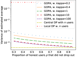
(a) Utility with respect to $\rho$

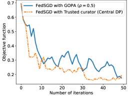
(b) A typical run of FedSGD

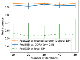
(c) Test accuracy of FedSGD

Figure 2: Comparing Gopa to central and local DP. Left: Utility of Gopa (measured by the variance of the estimated average) w.r.t. $\rho$. Middle: Evolution of the objective for a typical run of FedSGD. Right: Test accuracy of models learned with FedSGD. See text for details.

9 Conclusion

We proposed Gopa, a protocol to privately compute averages over the values of many users. Gopa satisfies DP, can nearly match the utility of a trusted curator, and is robust to malicious parties. It can be used in distributed and federated ML Jayaraman2018 ; kairouz2019advances in place of more costly secure aggregation schemes. In future work, we plan to provide efficient implementations, to integrate our approach in complete ML systems, and to exploit scaling to reduce the cost per average. We think that our work is also relevant beyond averaging, e.g. in the context of robust aggregation for distributed SGD Blanchard2017 and for computing pairwise statistics Bell2020a .

Declarations

This work was partially supported by ANR project ANR-20-CE23-0013 ’PMR’, ANR-20-CE23-0015 ’PRIDE’, and the ’Chair TIP’ project funded by ANR, I-SITE, MEL, ULille and INRIA. We thank Pierre Dellenbach and Alexandre Huat for the fruitful discussions. There are no conflicts of interest. No ethical approval was needed. As there were no participants no consent was needed to participate nor to publish. Code and data can be accessed by following the links in the text. The authors made approximately equal contributions.

Appendix Appendix A Proofs of Differential Privacy Guarantees

In this appendix, we provide derivations for our differential privacy guarantees.

A.1 Proof of Theorem 5.1

Theorem 5.1. Let $\varepsilon,\delta\in(0,1)$. Choose a vector $t=(t_{\eta},t_{\Delta})\in Z$ with $t_{\eta}=(t_{u})_{u\in U^{H}}$ and $t_{\Delta}=(t_{e})_{e\in E^{H}}$ such that $t_{\eta}+Kt_{\Delta}=X^{A}-X^{B}$ and let $\theta=t^{\top}\Sigma^{(-g)}t$. Under the setting introduced above, if $\theta\leq{\Theta_{max}}(\varepsilon,\delta)$ then Gopa is $(\varepsilon,\delta)$-DP, i.e.,

$$P({\hat{X}}\mid X^{A})\leq e^{\varepsilon}P({\hat{X}}\mid X^{B})+\delta.$$

Proof

We adapt ideas from Dwork2014a to our setting. First, we show that it is sufficient to prove that

$$P((\eta,\Delta))\leq P((\eta,\Delta)+t)e^{\varepsilon}+\delta.$$ (14)

In particular, if Eq (14) holds we have that

$$P(\hat{X}\mid X^{A}) =\int_{(\eta,\Delta)\in Z^{A}}P((\eta,\Delta))\text{d}\eta\text{d}\Delta$$

$$\leq\int_{(\eta,\Delta)\in Z^{A}}\left(P((\eta,\Delta)+t)e^{\varepsilon}+\delta\right)\text{d}\eta\text{d}\Delta$$

$$=\int_{(\eta,\Delta)-t\in Z^{A}}\left(P((\eta,\Delta))e^{\varepsilon}+\delta\right)\text{d}\eta\text{d}\Delta$$

$$=\int_{(\eta,\Delta)\in Z^{B}}\left(P((\eta,\Delta))e^{\varepsilon}+\delta\right)\text{d}\eta\text{d}\Delta$$

$$=P(\hat{X}\mid X^{B})e^{\varepsilon}+\delta,$$

which proves the required bound. Hence, it is sufficient to prove Eq (14), or else to prove that $P((\eta,\Delta))\leq e^{\varepsilon}P((\eta,\Delta)+t)$ with probability at least $1-\delta$. Denoting $\gamma=(\eta,\Delta)$ for convenience, we need to prove that with probability $1-\delta$ it holds that $|\log(P(\gamma)/P(\gamma+t))|\leq e^{\varepsilon}$. We have

$$\Big{|}\log\frac{P(\gamma)}{P(\gamma+t)}\Big{|} = \Big{|}-\frac{1}{2}\gamma^{\top}\Sigma^{(-g)}\gamma+\frac{1}{2}(\gamma+t)^{\top}\Sigma^{(-g)}(\gamma+t)\Big{|}$$

$$= \Big{|}\frac{1}{2}(2\gamma+t)^{\top}\Sigma^{(-g)}t\Big{|}.$$

To ensure that $|\log(P(\gamma)/P(\gamma+t))|\leq e^{\varepsilon}$ holds with probability at least $1-\delta$, since we are interested in the absolute value, we will show that

$$P\Big{(}\frac{1}{2}(2\gamma+t)^{\top}\Sigma^{(-g)}t\geq\varepsilon\Big{)}\leq\delta/2,$$

the proof of the other direction is analogous. This is equivalent to

$$P(\gamma\Sigma^{(-g)}t\geq\varepsilon-t^{\top}\Sigma^{(-g)}t/2)\leq\delta/2.$$ (15)

The variance of $\gamma\Sigma^{(-g)}t$ is

$$\text{var}(\gamma\Sigma^{(-g)}t) = \sum_{v}\text{var}\left(\eta_{v}\sigma_{\eta}^{-2}t_{v}\right)+\sum_{e}\text{var}\left(\Delta_{e}\sigma_{\Delta}^{-2}t_{e}\right)$$

$$= \sum_{v}\text{var}\left(\eta_{v}\right)\sigma_{\eta}^{-4}t_{v}^{2}+\sum_{e}\text{var}\left(\Delta_{e}\right)\sigma_{\Delta}^{-4}t_{e}^{2}$$

$$= \sum_{v}\sigma_{\eta}^{2}\sigma_{\eta}^{-4}t_{v}^{2}+\sum_{e}\sigma_{\Delta}^{2}\sigma_{\Delta}^{-4}t_{e}^{2}$$

$$= \sum_{v}\sigma_{\eta}^{-2}t_{v}^{2}+\sum_{e}\sigma_{\Delta}^{-2}t_{e}^{2}$$

$$= t^{\top}\Sigma^{(-g)}t.$$

For any centered Gaussian random variable $Y$ with variance $\sigma_{Y}^{2}$, we have that

$$P(Y\geq\lambda)\leq\frac{\sigma_{Y}}{\lambda\sqrt{2\pi}}\exp\left(-\lambda^{2}/2\sigma_{Y}^{2}\right).$$ (16)

Let $Y=\gamma\Sigma^{(-g)}t$, $\sigma_{Y}^{2}=t^{\top}\Sigma^{(-g)}t$ and $\lambda=\varepsilon-t^{\top}\Sigma^{(-g)}t/2$, then satisfying

$$\frac{\sigma_{Y}}{\lambda\sqrt{2\pi}}\exp\left(-\lambda^{2}/2\sigma_{Y}^{2}\right)\leq\delta/2$$ (17)

implies (15). Equation (17) is equivalent to

$$\frac{\lambda}{\sigma_{Y}}\exp\left(\lambda^{2}/2\sigma_{Y}^{2}\right)\geq 2/\delta\sqrt{2\pi},$$

or, after taking logarithms on both sides, to

$$\log\left(\frac{\lambda}{\sigma_{Y}}\right)+\frac{1}{2}\left(\frac{\lambda}{\sigma_{Y}}\right)^{2}\geq\log\left(\frac{2}{\delta\sqrt{2\pi}}\right).$$

To make this inequality hold, we require

$$\log\left(\frac{\lambda}{\sigma_{Y}}\right)\geq 0$$ (18)

and

$$\frac{1}{2}\left(\frac{\lambda}{\sigma_{Y}}\right)^{2}\geq\log\left(\frac{2}{\delta\sqrt{2\pi}}\right).$$ (19)

Equation (18) is equivalent to $\lambda\geq\sigma_{Y}.$ Substituting $\lambda$ and $\sigma_{Y}$ we get

$$\varepsilon-t^{\top}\Sigma^{(-g)}t/2\geq(t^{\top}\Sigma^{(-g)}t)^{1/2},$$

which is equivalent to (4). Substituting $\lambda$ and $\sigma_{Y}$ in Equation (19) gives (5). Hence, if Equations (4) and (5) are satisfied the desired differential privacy follows.∎

A.2 Proofs for Section 5.1.3

Lemma 1. In the setting described above, for any $t$ chosen as in Theorem 5.1 we have:

$$\sum_{u\in U^{H}}t_{u}=1.$$

Proof

Due to the properties of the incidence matrix $K$, i.e., $\forall u,v:K_{u,\{u,v\}}=-K_{v,\{u,v\}}$, the sum of the components of the vector $K\Delta$ is zero, i.e.,

$$\sum_{u\in U^{H}}\left(K\Delta\right)_{u}=\sum_{u\in U^{H}}\left(\sum_{\{u,v\}\in E^{H}}K_{u,\{u,v\}}\Delta_{\{u,v\}}\right)_{u}=0$$

Combining this with the fact that $t_{\eta}+Kt_{\Delta}=X^{A}-X^{B}$ with $\sum_{u\in U^{H}}(X^{A}-X^{B})_{u}=1$ we obtain Equation (6). ∎

Lemma 2. In the setting described above with $t$ as defined in Theorem 5.1, if $t_{\eta}=\mathbbm{1}_{n_{H}}/n_{H}$, then $G^{H}$ must be connected.

Proof

Suppose $G^{H}$ is not connected, then there is a connected component $C\subseteq U^{H}\setminus\{v_{1}\}$. Let $t_{C}=\left(t_{u}\right)_{u\in C}$ and $\Delta_{C}=(\Delta_{e})_{e\in{{\vec{E}}^{H}}\cap(C\times C)}$. Let $K_{C}=\left(K_{u,e}\right)_{u\in C,e\in{{\vec{E}}^{H}}\cap(C\times C)}$ be the incidence matrix of $G^{H}[C]$, the subgraph of $G^{H}$ induced by $C$. Due to the properties of the incidence matrix of a graph there would hold $\sum_{u\in C}(K_{C}\Delta_{C})_{u}=0$. As there would be no edges between vertices in $C$ and vertices outside $C$, we would have $\sum_{u\in C}(K\Delta)_{u}=0$. There would follow $\sum_{u\in C}t_{u}=\sum_{u\in C}(X^{A}-X^{B}-K\Delta)_{u}=0$ which would contradict with $t_{\eta}=\mathbbm{1}_{n_{H}}/n_{H}$. In conclusion, $G^{H}$ must be connected. ∎

A.3 Random $k$-out Graphs

In this section, we will study the differential privacy properties for the case where all users select $k$ neighbors randomly, leading to a proof of Theorem 5.4. We will start by analyzing the properties of $G^{H}$ (Section A.3.1). Section A.3.2 consists of preparations for embedding a suitable spanning tree in $G^{H}$. Next, in Section A.3.3 we will prove a number of lemmas showing that such suitable spanning tree can be embedded almost surely in $G^{H}$. Finally, we will apply these results to proving differential privacy guarantees for Gopa when communicating over such a random $k$-out graph $G$ in Section A.3.4, proving Theorem 5.4.

In this section, all newly introduced notations and definitions are local and will not be used elsewhere. At the same time, to follow more closely existing conventions in random graph theory, we may reuse in this section some variable names used elsewhere and give them a different meaning.

A.3.1 The Random Graph $G^{H}$

Recall that the communication graph $G^{H}$ is generated as follows:

• We start with $n=|U|$ vertices where $U$ is the set of agents.

• All (honest) agents randomly select $k$ neighbors to obtain a $k$-out graph $G$.

• We consider the subgraph $G^{H}$ induced by the set $U^{H}$ of honest users who did not drop out. Recall that $n_{H}=|U^{H}|$ and that a fraction $\rho$ of the users is honest and did not drop out, hence $n_{H}=\rho n$.

Let $k_{H}=\rho k$. The graph $G^{H}$ is a subsample of a $k$-out-graph, which for larger $n_{H}$ and $k_{H}$ follows a distribution very close to that of Erdős-Rényi random graphs $G_{p}(n_{H},2k_{H}/n_{H})$. To simplify our argument, in the sequel we will assume $G^{H}$ is such random graph as this does not affect the obtained result. In fact, the random $k$-out model concentrates the degree of vertices more narrowly around the expected value than Erdős-Rényi random graphs, so any tail bound our proofs will rely on that holds for Erdős-Rényi random graphs also holds for the graph $G^{H}$ we are considering. In particular, for $v\in U^{H}$, the degree of $v$ is a random variable which we will approximate for sufficiently large $n_{H}$ and $k_{H}$ by a binomial $B(n_{H},2k_{H}/n_{H})$ with expected value $2k_{H}$ and variance $2k_{H}(1-2k_{H}/n_{H})\approx 2k_{H}$.

A.3.2 The Shape of the Spanning Tree

Remember that our general strategy to prove differential privacy results is to find a spanning tree in $G^{H}$ and then to compute the norm of the vector $t_{\Delta}$ that will “spread” the difference between $X^{A}$ and $X^{B}$ over all vertices (so as to get a $\sigma_{\eta}$ of the same order as in the trusted curator setting). Here, we will first define the shape of a rooted tree and then prove that with high probability this tree is isomorphic to a spanning tree of $G^{H}$. Of course, we make a crude approximation here, as in the (unlikely) case that our predefined tree cannot be embedded in $G^{H}$ it is still possible that other trees could be embedded in $G^{H}$ and would yield similarly good differentially privacy guarantees. While our bound on the risk that our privacy guarantee does not hold will not be tight, we will focus on proving our result for reasonably-sized $U$ and $k$, and on obtaining interesting bounds on the norm of $t_{\Delta}$.

Let $G^{H}=([n_{H}],E^{H})$ be a random graph where between every pair of vertices there is an edge with probability $2k_{H}/n_{H}$. The average degree of $G^{H}$ is $2k_{H}$.

Let $k_{H}\geq 4$. Let $q\geq 3$ be an integer. Let $\Delta_{1}$, $\Delta_{2}$ …$\Delta_{q}$ be a sequence of positive integers such that

$$\left(\sum_{i=1}^{q}\prod_{j=1}^{i}\Delta_{j}\right)-(\Delta_{q}+1)\prod_{j=1}^{q-2}\Delta_{j}<n_{H}\leq\sum_{i=1}^{q}\prod_{j=1}^{i}\Delta_{j}.$$ (20)

Let $T=([n_{H}],E_{T})$ be a balanced rooted tree with $n_{H}$ vertices, constructed as follows. First, we define for each level $l$ a variable $z_{l}$ representing the number of vertices at that level, and a variable $Z_{l}$ representing the total number of vertices in that and previous levels. In particular: at the root $Z_{-1}=0$, $Z_{0}=z_{0}=1$ and for $l\in[q-2]$ by induction $z_{l}=z_{l-1}\Delta_{l}$ and $Z_{l}=Z_{l-1}+z_{l}$. Then, $z_{q-1}=\lceil(n_{H}-Z_{q-2})/(\Delta_{q}+1)\rceil$, $Z_{q-1}=Z_{q-2}+z_{q-1}$, $z_{q}=n_{H}-Z_{q-1}$ and $Z_{q}=n_{H}$. Next, we define the set of edges of $T$:

$$E_{T}=\{\{Z_{l-2}+i,Z_{l-1}+z_{l-1}j+i\}\mid l\in[q]\wedge i\in[z_{l-1}]\wedge z_{l-1}j+i\in[z_{l}]\}.$$

So the tree consists of three parts: in the first $q-2$ levels, every vertex has a fixed, level-dependent number of children, the last level is organized such that a maximum of parents has $\Delta_{q}$ children, and in level $q-1$ parent nodes have in general $\Delta_{q-1}-1$ or $\Delta_{q-1}$ children. Moreover, for $0\leq l\leq q-2$, the difference between the number of vertices in the subtrees rooted by two vertices in level $l$ is at most $\Delta_{q}+2$. We also define the set of children of a vertex, i.e., for $l\in[q]$ and $i\in[z_{l-1}]$,

$$ch(Z_{l-2}+i)=\{Z_{l-1}+z_{l-1}j+i\mid z_{l-1}j+i\in[z_{l}]\}.$$

In Section A.3.3, we will show conditions on $n_{H}$, $\Delta_{1}\ldots\Delta_{q}$, $k_{H}$ and $\delta$ such that for a random graph $G^{H}$ on $n_{H}$ vertices and a vertex $v_{1}$ of $G^{H}$, with high probability (at least $1-\delta$) $G^{H}$ contains a subgraph isomorphic to $T$ whose root is at $v_{1}$.

A.3.3 Random Graphs Almost Surely Embed a Balanced Spanning Tree

The results below are inspired by Krivelevich2010 . We specialize this result to our specific problem, obtaining proofs which are also valid for graphs smaller than $10^{10}$ vertices, even if the bounds get slightly weaker when we drop terms of order $O(\log(\log(n_{H})))$ for the simplicity of our derivation.

Let $F$ be the subgraph of $T$ induced by all its non-leafs, i.e., $F=([Z_{q-1}],E_{F})$ with $E_{F}=\{\{i,j\}\in E_{T}\mid i,j\leq Z_{q-1}\}$.

Lemma 3

Let $G^{H}$ and $F$ be defined as above. Let $v_{1}$ be a vertex of $G^{H}$. Let $n_{H}\geq k_{H}\geq\Delta_{i}\geq 3$ for $i\in[l]$. Let $\gamma=\max_{l=1}^{q-1}\Delta_{l}/k_{H}$ and let $\gamma+4(\Delta_{q}+2)^{-1}+2n_{H}^{-1}\leq 1$. Let $k_{H}\geq 4\log(2n_{H}/\delta_{F}(\Delta_{q}+2))$. Then, with probability at least $1-\delta_{F}$, there is an isomorphism $\phi$ from $F$ to a subgraph of $G^{H}$, mapping the root $1$ of $F$ on $v_{1}$.

Proof

We will construct $\phi$ by selecting images for the children of vertices of $F$ in increasing order, i.e., we first select $\phi(1)=v_{1}$, then map children $\{2\ldots\Delta_{1}+1\}$ of $1$ to vertices adjacent to $v_{1}$, then map all children of $2$ to vertices adjacent to $\phi(2)$, etc. Suppose we are processing level $l\in[q-1]$ and have selected $\phi(j)$ for all $j\in ch(i^{\prime})$ for all $i^{\prime}<i$ for some $Z_{l-1}<i\leq Z_{l}$. We now need to select images for the $\Delta_{l}$ children $j\in ch(i)$ of vertex $i$ (or in case $l=q-1$ possibly only $\Delta_{l}-1$ children). This means we need to find $\Delta_{l}$ neighbors of $i$ not already assigned as image to another vertex (i.e., not belonging to $\cup_{0\leq i^{\prime}<i}\phi(ch(i^{\prime}))$). We compute the probability that this fails. For any vertex $j\in[n_{H}]$ with $i\neq j$, the probability that there is an edge between $i$ and $j$ in $G^{H}$ is $2k_{H}/n_{H}$. Therefore, the probability that we fail to find $\Delta_{l}$ free neighbors of $i$ can be upper bounded as

$$Pr\left[\text{{Fail}}_{F}(i)\right]=Pr\left[\text{Bin}\left(n_{H}-Z_{l},\frac{2k_{H}}{n_{H}}\right)<\Delta_{l}\right]\leq\exp\left(\frac{-\left((n_{H}-Z_{l})\frac{2k_{H}}{n_{H}}-\Delta_{l}\right)^{2}}{2(n_{H}-Z_{l})\frac{2k_{H}}{n_{H}}}\right).$$ (21)

We know that $n_{H}-Z_{l}\geq z_{q}$. Moreover, $(z_{q}+\Delta_{q}-1)/\Delta_{q}\geq z_{q-1}$ and $Z_{q-2}+1\leq z_{q-1}$, hence $2(z_{q}+\Delta_{q}-1)/\Delta_{q}\geq Z_{q-2}+z_{q-1}+1=Z_{q-1}+1$ and $2(z_{q}+\Delta_{q}-1)/\Delta_{q}+z_{q}\geq n_{H}+1$. There follows

$$z_{q}(2+\Delta_{q})\geq n_{H}+1-2(\Delta_{q}-1)/\Delta_{q}\geq n_{H}-1.$$

Therefore,

$$n_{H}-Z_{l}\geq z_{q}\geq n_{H}(1-2(\Delta_{q}+2)^{-1}-n_{H}^{-1}).$$ (22)

Substituting this and $\Delta_{l}\geq\gamma k_{H}$ in Equation (21), we get

$$Pr\left[\text{{Fail}}_{F}(i)\right] \leq \exp\left(\frac{-\left(n_{H}(1-2(\Delta_{q}+2)^{-1}-n_{H}^{-1})\frac{2k_{H}}{n_{H}}-k_{H}\gamma\right)^{2}}{2n_{H}(1-2(\Delta_{q}+2)^{-1}-n_{H}^{-1})\frac{2k_{H}}{n_{H}}}\right)$$

$$\leq \exp\left(\frac{-k_{H}^{2}\left(2(1-2(\Delta_{q}+2)^{-1}-n_{H}^{-1})-\gamma\right)^{2}}{4k_{H}}\right)$$

$$\leq \exp\left(\frac{-k_{H}^{2}}{4k_{H}}\right)=\exp\left(\frac{-k_{H}}{4}\right),$$

where the latter inequality holds as $\gamma+4(\Delta_{q}+2)^{-1}+2n_{H}^{-1}\leq 1$. As $k_{H}\geq 4\log(2n_{H}/\delta_{F}(\Delta_{q}+2))$ we can conclude that

$$Pr\left[\text{{Fail}}_{F}(i)\right]\leq\frac{\delta_{F}(\Delta_{q}+2)}{2n_{H}}.$$

The total probability of failure to embed $F$ in $G^{H}$ is therefore given by

$$\sum_{i=2}^{Z_{q-1}}\text{{Fail}}_{F}(i) \leq (Z_{q-1}-1)\frac{\delta_{F}(\Delta_{q}+2)}{2n_{H}}$$

$$\leq \left(n_{H}(2(\Delta_{q}+2)^{-1}+n_{H}^{-1})-1\right)\frac{\delta_{F}(\Delta_{q}+2)}{2n_{H}}=\frac{2n_{H}}{\Delta_{q}+2}\frac{\delta_{F}(\Delta_{q}+2)}{2n_{H}}=\delta_{F},$$

where we again applied (22).∎

Now that we can embed $F$ in $G^{H}$, we still need to embed the leaves of $T$. Before doing so, we review a result on matchings in random graphs. The next lemma mostly follows Bollobas2001a (Theorem 7.11 therein), we mainly adapt to our notation, introduce a confidence parameter and make a few less crude approximations.

Lemma 4

Let $m\geq 27$ (in our construction, $m=z_{q}$) and $\zeta\geq 4$. Consider a random bipartite graph with vertex partitions $A=\{a_{1}\ldots a_{m}\}$ and $B=\{b_{1}\ldots b_{m}\}$, where for every $i,j\in[m]$ the probability of an edge $\{a_{i},b_{j}\}$ is $p=\zeta(\log(m){})/m$. Then, the probability of a complete matching between $A$ and $B$ is higher than

$$1-\frac{em^{-2(\zeta-1)/3}}{1-m^{-(\zeta-1)/3}}.$$

Proof

For a set $X$ of vertices, let $\Gamma(X)$ be the set of all vertices adjacent to at least one member of $X$. Then, if there is no complete matching between $A$ and $B$, there is some set $X$, with either $X\subset A$ or $X\subset B$, which violates Hall’s condition, i.e., $|\Gamma(X)|<|X|$. Let $X$ be the smallest set satisfying this property (so the subgraph induced by $X\cup\Gamma(X)$ is connected). The probability that such sets $X$ and $\Gamma(X)$ of respective sizes $i$ and $j=|\Gamma(X)|$ exist is upper bounded by appropriately combining:

• the number of choices for $X$, i.e., $2$ (for selecting $A$ or $B$) times $\left(\begin{array}[]{c}{m}\\ {i}\end{array}\right)$,

• the number of choices for $\Gamma(X)$, i.e., $\left(\begin{array}[]{c}{m}\\ {i-1}\end{array}\right)$ (considering that $j\leq i-1$),

• an upper bound for the probability that under these choices of $X$ and $\Gamma(X)$ there are at least $2i-2$ edges (as the subgraph induced by $X\cup\Gamma(X)$ is connected), i.e., $\left(\begin{array}[]{c}{ij}\\ {i+j-1}\end{array}\right)$ possible choices of the vertex pairs and $p^{i+j-1}$ the probability that these vertex pairs all form edges, and

• the probability that there is no edge between any of $X\cup\Gamma(X)$ and the other vertices, i.e., $(1-p)^{i(m-j)+j(m-i)}=(1-p)^{m(i+j)-2ij}$.

Thus, we upper bound the probability of observing such sets $X$ and $\Gamma(X)$ of sizes $i$ and $j$ as follows:

$$\text{{Fail}}_{B}(i,j) \leq \left(\begin{array}[]{c}{m}\\ {i}\end{array}\right)\left(\begin{array}[]{c}{m}\\ {j}\end{array}\right)\left(\begin{array}[]{c}{ij}\\ {i+j-1}\end{array}\right)p^{i+j-1}(1-p)^{m(i+j)-2ij}$$

$$\leq \left(\frac{me}{i}\right)^{i}\left(\frac{me}{j}\right)^{j}\left(\frac{ije}{i+j-1}\right)^{i+j-1}p^{i+j-1}(1-p)^{m(i+j)-2ij}.$$

Here, in the second line the classic upper bound for combinations is used: $\left(\begin{array}[]{c}{m}\\ {i}\end{array}\right)<\left(\frac{me}{i}\right)^{i}$. As $2j\leq i+j-1$, we get

$$\text{{Fail}}_{B}(i,j) \leq \left(\frac{me}{i}\right)^{i}\left(\frac{me}{j}\right)^{j}\left(\frac{ie}{2}\right)^{i+j-1}p^{i+j-1}(1-p)^{m(i+j)-2ij}$$ (30)

$$\leq \frac{m^{i+j}e^{2i+2j-1}i^{j-1}}{j^{j}2^{i+j-1}}p^{i+j-1}(1-p)^{m(i+j)-2ij}.$$

As $0<p<1$, there also holds

$$(1-p)^{1/p}<1/e,$$

and therefore

$$(1-p)^{m(i+j)-2ij}=(1-p)^{\frac{1}{p}p(m(i+j)-2ij)}<(1/e)^{p(m(i+j)-2ij)}.$$

We can substitute $p=\zeta(\log(m){})/m$ to obtain

$$(1-p)^{m(i+j)-2ij} < (1/e)^{(\zeta(\log(m){})/m)(m(i+j)-2ij)}=\left(\frac{{1}}{m}\right)^{\zeta(m(i+j)-2ij)/m}.$$

Substituting this into Equation (30), we get

$$\text{{Fail}}_{B}(i,j) \leq \frac{m^{i+j}e^{2i+2j-1}i^{j-1}}{j^{j}2^{i+j-1}}\left(\frac{\log(m)\zeta}{m}\right)^{i+j-1}\left(\frac{{1}}{m}\right)^{\zeta(m(i+j)-2ij)/m}$$

$$= \frac{mei^{j-1}}{j^{j}}\left(\frac{\log(m)\zeta e^{2}}{2}\right)^{i+j-1}\left(\frac{{1}}{m}\right)^{\zeta((i+j)-2ij/m)}.$$

Given that $m^{\zeta/3}\geq\zeta\log(m){}e^{2}/2$ holds for $m\geq 27$ and $\zeta\geq 4$, we get

$$\text{{Fail}}_{B}(i,j) \leq \frac{mei^{j-1}}{j^{j}}\left(\frac{\log(m){}\zeta e^{2}}{2m^{\zeta/3}}\right)^{i+j-1}m^{-\zeta((i+j)-2ij/m)+\zeta(i+j-1)/3}$$

$$\leq \frac{ei^{j-1}}{j^{j}}m^{-\zeta(\frac{2}{3}(i+j)+1/3-2ij/m)+1}$$

$$\leq \frac{ei^{j-1}}{j^{j}}m^{-\zeta(\frac{1}{3}i+\frac{1}{3})+1}.$$

As $\zeta\geq 4$, this implies

$$\text{{Fail}}_{B}(i,j) \leq \frac{e}{i}\left(\frac{i}{j}\right)^{j}m^{-\frac{\zeta i}{3}-\frac{1}{3}}.$$ (31)

There holds:

$$\sum_{j=1}^{i-1}\left(\frac{i}{j}\right)^{j} = \sum_{j=1}^{\lfloor i/3\rfloor}\left(\frac{i}{j}\right)^{j}+\sum_{j=\lfloor i/3\rfloor+1}^{i}\left(\frac{i}{j}\right)^{j}$$

$$\leq \sum_{j=1}^{\lfloor i/3\rfloor}\left(\frac{i}{j}\right)^{j}+\sum_{j=\lfloor i/3\rfloor+1}^{i}3^{j}=\sum_{j=1}^{\lfloor i/3\rfloor}\left(\frac{i}{j}\right)^{j}+3^{\lfloor i/3\rfloor+1}\frac{3^{i-\lfloor i/3\rfloor}-1}{3-1}$$

$$< \sum_{j=1}^{\lfloor i/3\rfloor}\left(\frac{i}{j}\right)^{j}+\frac{3^{i+1}}{2}<\sum_{j=1}^{\lfloor i/3\rfloor}i^{i/3}+\frac{3^{i+1}}{2}$$

$$\leq \frac{i}{3}i^{i/3}+\frac{3^{i+1}}{2}.$$

Substituting in Equation (31) gives

$$\text{{Fail}}_{B} = \sum_{i=2}^{m/2}\sum_{j=1}^{i-1}\text{{Fail}}_{B}(i,j)$$

$$< \sum_{i=2}^{m/2}\sum_{j=1}^{i-1}\frac{e}{i}\left(\frac{i}{j}\right)^{j}m^{-\frac{\zeta i}{3}-\frac{1}{3}}<\sum_{i=2}^{m/2}\left(\frac{i^{i/3+1}}{3}+\frac{3^{i+1}}{2}\right)\frac{e}{i}m^{-\frac{\zeta i}{3}-\frac{1}{3}}$$

$$< \sum_{i=2}^{m/2}\left(i^{i/3}+3^{i+1}\right)\frac{e}{2}m^{-\frac{\zeta i}{3}-\frac{1}{3}}<\sum_{i=2}^{m/2}i^{i/3}\frac{e}{2}m^{-\frac{\zeta i}{3}-\frac{1}{3}}+3^{i+1}\frac{e}{2}m^{-\frac{\zeta i}{3}-\frac{1}{3}}.$$

As $m\geq 27=3^{3}$ we can now write

$$\text{{Fail}}_{B} < \frac{e}{2}\sum_{i=2}^{m/2}m^{-\frac{(\zeta-1)i}{3}-\frac{1}{3}}+m^{(i+1)/3}m^{-\frac{\zeta i}{3}-\frac{1}{3}}<\frac{e}{2}\sum_{i=2}^{m/2}m^{-\frac{(\zeta-1)i}{3}-\frac{1}{3}}+m^{-\frac{(\zeta-1)i}{3}}$$

$$< e\sum_{i=2}^{m/2}m^{-\frac{(\zeta-1)i}{3}}=em^{-\frac{2(\zeta-1)}{3}}\sum_{i=0}^{m/2-2}\left(m^{-\frac{\zeta-1}{3}}\right)^{i}$$

$$= em^{-\frac{2(\zeta-1)}{3}}\frac{1-\left(m^{-\frac{\zeta-1}{3}}\right)^{m/2-1}}{1-\left(m^{-\frac{\zeta-1}{3}}\right)}<em^{-\frac{2(\zeta-1)}{3}}\frac{1}{1-\left(m^{-\frac{\zeta-1}{3}}\right)}.$$

This concludes the proof.∎

Lemma 5

Let $m\geq 27$ and $\delta_{B}>0$. Let

$$\zeta=\max\left(4,1+\frac{3\log(2e/\delta_{B})}{2\log(m)}\right).$$

Consider a random bipartite graph as described in Lemma 4 above. Then, with probability at least $1-\delta_{B}$ there is a complete matching between $A$ and $B$.

Proof

From the given $\zeta$, we can infer that

$$\zeta-1\geq\frac{3\log(2e/\delta_{B})}{2\log(m)}$$

$$\zeta-1\geq\frac{-3\log\left(\delta_{B}/2e\right)}{2\log(m)}$$

$$-\frac{2}{3}(\zeta-1)\log(m)\leq\log\left(\delta_{B}/2e\right)$$

$$m^{-2(\zeta-1)/3}\leq\delta_{B}/2e$$

We also know that $\zeta\geq 4$ and $m\geq 27$, hence $(\zeta-1)/3\geq 1$ and $1-m^{-(\zeta-1)/3}\geq 26/27\geq 1/2$. We know from Lemma 4 that the probability of having a complete matching is at least

$$1-\frac{em^{-2(\zeta-1)/3}}{1-m^{-(\zeta-1)/3}}\geq 1-\frac{e(\delta_{B}/2e)}{1/2}=1-\delta_{B}.$$

Lemma 6

Let $\delta_{B}>0$, $\Delta\geq 1$ (in our construction, $\Delta=\Delta_{q}$) and $m\geq 27$. Let $d_{1}\ldots d_{l}$ be positive numbers, with $d_{i}=\Delta$ for $i\in[l-1]$, $d_{l}\in[\Delta]$ and $\sum_{i=1}^{l}d_{i}=m$. Let $A=\{a_{1}\ldots a_{l}\}$ and $B=\{b_{1}\ldots b_{m}\}$ be disjoint sets of vertices in a random graph $G^{H}$ where the probability to have an edge $\{a_{i},b_{j}\}$ is $p=2k_{H}/n_{H}$ for any $i$ and $j$. Let

$$p\geq 1-\left(1-\max\left(4,1+\frac{3\log(2e/\delta_{B})}{2\log(m)}\right)\frac{\log(m)}{m}\right)^{\Delta}.$$ (32)

Then with probability at least $1-\delta_{B}$, $G^{H}$ contains a collection of disjoint $d_{i}$-stars with centers $a_{i}$ and leaves in $B$.

Proof

Define an auxiliary random bipartite graph ${G^{\prime}}$ with sides $A^{\prime}=\{a^{\prime}_{1}\ldots a^{\prime}_{m}\}$ and $B=\{b_{1}\ldots b_{m}\}$. For every $i,j\in[m]$, the probability of having an edge between $a_{i}$ and $b_{j}$ in ${G^{\prime}}$ is ${p^{\prime}}=1-(1-p)^{1/\Delta}$. We relate the distributions on the edges of $G^{H}$ and ${G^{\prime}}$ by requiring there is an edge between $a_{i}$ and $b_{j}$ if and only if there is an edge between $a^{\prime}_{\Delta(i-1)+i^{\prime}}$ and $b_{j}$ for all $i^{\prime}\in[\Delta]$.

From Equation (32) we can derive

$${p^{\prime}}\geq\max\left(4,1+\frac{3\log(2e/\delta_{B})}{2\log(m)}\right)\frac{\log(m)}{m}.$$ (33)

Setting

$$\zeta=\max\left(4,1+\frac{3\log(2e/\delta_{B})}{2\log(m)}\right),$$

this ensures ${p^{\prime}}$ satisfies the constraints of Lemma 5:

$${p^{\prime}}=\zeta\log(m)/m.$$

As a result, there is a complete matching in ${G^{\prime}}$ with probability at least $1-\delta_{B}$, and hence the required stars can be found in $G^{H}$ with probability at least $1-\delta_{B}$. ∎

Lemma 7

Let $\delta_{F}>0$ and $\delta_{B}>0$. Let $G^{H}$ and $T$ and their associated variables be as defined above. Assume that the following conditions are satisfied:

$$(a) n_{H}\geq 27(\Delta_{q}+2)/\Delta_{q},$$

$$(b) \gamma+2(\Delta_{q}+2)^{-1}+n_{H}^{-1}\leq 1,$$

$$(c) k_{H}\geq 4\log(2n_{H}/\delta_{F}(\Delta_{q}+2)),$$

$$(d) k_{H}\geq\max\left(4,1+\frac{3\log(2e/\delta_{B})}{2\log(n_{H}\Delta_{q}/(\Delta_{q}+2))}\right)\frac{\Delta_{q}+2}{2}\log\left(\frac{n_{H}\Delta_{q}}{\Delta_{q}+2}\right),$$

$$(e) \gamma=\max{}_{l=1}^{q-1}\Delta_{l}/k_{H}.$$

Let $G^{H}$ be a random graph where there is an edge between any two vertices with probability $p$. Let $v_{1}$ be a vertex of $G^{H}$. Then, with probability at least $1-\delta_{F}-\delta_{B}$, there is a subgraph isomorphism between the tree $T$ defined above and $G^{H}$ such that the root of $T$ is mapped on $v_{1}$.

Proof

The conditions of Lemma 3 are clearly satisfied, so with probability $1-\delta_{F}$ there is a tree isomorphic to $F$ in $G^{H}$. Then, from condition (d) above and knowing that the edge probability is $p=2k_{H}/n_{H}$, we obtain

$$p\geq\max\left(4,1+\frac{3\log(2e/\delta_{B})}{2\log(n_{H}\Delta_{q}/(\Delta_{q}+2))}\right)\frac{1}{n_{H}\Delta_{q}/(\Delta_{q}+2)}\log\left(\frac{n_{H}\Delta_{q}}{\Delta_{q}+2}\right)\Delta_{q}.$$

Taking into account that $m=n_{H}\Delta_{q}/(\Delta_{q}+2)$, we get

$$p\geq\max\left(4,1+\frac{3\log(2e/\delta_{B})}{2\log(m)}\right)\frac{1}{m}\log\left(m\right)\Delta_{q},$$

which implies the condition on $p$ in Lemma 5. The other conditions of that lemma can be easily verified. As a result, with probability at least $1-\delta_{B}$ there is a set of stars in $G^{H}$ linking the leaves of $F$ to the leaves of $T$, so we can embed $T$ completely in $G^{H}$. ∎

A.3.4 Running Gopa on Random Graphs

Assume we run Gopa on a random graph satisfying the properties above, what can we say about the differential privacy guarantees? According to Theorem  5.1, it is sufficient that there exists a spanning tree and vectors $t_{\eta}$ and $t_{\Delta}$ such that $t_{\eta}+Kt_{\Delta}=X^{A}-X^{B}$. We fix $t_{\eta}$ in the same way as for the other discussed topologies (see sections 5.2 and 5.3) in order to achieve the desired $\sigma_{\eta}$ and focus our attention on $t_{\Delta}$. According to Lemma 7, with high probability there exists in $G^{H}$ a spanning tree rooted at the vertex where $X^{A}$ and $X^{B}$ differ and a branching factor $\Delta_{l}$ specified per level. So given a random graph on $n_{H}$ vertices with edge density $2k_{H}/n_{H}$, if the conditions of Lemma 7 are satisfied we can find such a tree isomorphic to $T$ in the communication graph between honest users $G^{H}$. In many cases (reasonably large $n_{H}$ and $k_{H}$), this means that the lemma guarantees a spanning tree with branching factor as high as $O(k_{H})$, even though it may be desirable to select a small value for the branching factor of the last level in order to more easily satisfy condition (d) of Lemma 7, e.g., $\Delta_{q}=2$ or even $\Delta_{q}=1$.

Lemma 8

Under the conditions described above,

$$t_{\Delta}^{\top}t_{\Delta} \leq \frac{1}{\Delta_{1}}\left(1+\frac{1}{\Delta_{2}}\left(1+\frac{1}{\Delta_{3}}\left(\ldots\frac{1}{\Delta_{q}}\right)\right)\right)+\frac{(\Delta_{q}+2)(\Delta_{q}+2+2q)}{n_{H}}$$

$$\leq \frac{1}{\Delta_{1}}\left(1+\frac{2}{\Delta_{2}}\right)+O(n_{H}^{-1}).$$

Proof

Let $q$ be the depth of the tree $T$. The tree is balanced, so in every node the number of vertices in the subtrees of its children differs in at most $\Delta_{q}+2$. For edges $e$ incident with the root (at level 0 node), $|t_{e}-\Delta_{1}^{-1}|\leq n_{H}^{-1}(\Delta_{q}+2)$. In general, for a node at level $l$ (except leaves or parents of leaves), there are $\prod_{i=1}^{l}\Delta_{i}$ vertices, each of which have $\Delta_{l+1}$ children, and for every edge $e$ connecting such a node with a child,

$$\left|t_{e}-\prod_{i=1}^{l+1}\Delta_{i}^{-1}\right|\leq(\Delta_{q}+2)/n_{H}.$$

For a complete tree (of $1+\Delta+\ldots+\Delta^{q}$ vertices), we would have

$$t_{\Delta}^{\top}t_{\Delta} = \sum_{l=1}^{q}\prod_{i=1}^{l}\Delta_{i}\left(\prod_{i=1}^{l}\Delta_{i}^{-1}\right)^{2}=\sum_{l=1}^{q}\left(\prod_{i=1}^{l}\Delta_{i}\right)^{-1},$$

which corresponds to the first term in Equation (8). As the tree may not be complete, i.e., there may be less than $\prod_{i=1}^{q}\Delta_{i}$ leaves, we analyze how much off the above estimate is. For an edge $e$ connecting a vertex of level $l$ with one of its children,

$$\left|t_{e}-\prod_{i=1}^{l+1}\Delta_{i}\right|\leq(\Delta_{q}+2)/n_{H},$$

and hence

$$\left|t_{e}^{2}-\left(\prod_{i=1}^{l+1}\Delta_{i}\right)^{2}\right| \leq \left|t_{e}-\prod_{i=1}^{l+1}\Delta_{i}\right|\left(t_{e}+\prod_{i=1}^{l+1}\Delta_{i}\right)$$

$$\leq \frac{\Delta_{q}+2}{n_{H}}\left(t_{e}-\prod_{i=1}^{l+1}\Delta_{i}+2\prod_{i=1}^{l+1}\Delta_{i}\right)$$

$$\leq \left(\frac{\Delta_{q}+2}{n_{H}}\right)^{2}+2\frac{\Delta_{q}+2}{n_{H}}\prod_{i=1}^{l+1}\Delta_{i}.$$

Summing over all edges gives

$$t_{\Delta}^{\top}t_{\Delta}-\sum_{l=1}^{q}\left(\prod_{i=1}^{l}\Delta_{i}\right)^{-1} \leq \sum_{l=1}^{q}z_{l}\left((\Delta_{q}+2)/n_{H}^{2}+2\left(\prod_{i=1}^{l+1}\Delta_{i}\right)^{-1}(\Delta_{q}+2)/n_{H}\right)$$

$$= (\Delta_{q}+2)^{2}/n_{H}+\sum_{l=1}^{q}2z_{l}\left(\prod_{i=1}^{l+1}\Delta_{i}\right)^{-1}(\Delta_{q}+2)/n_{H}$$

$$\leq (\Delta_{q}+2)^{2}/n_{H}+\sum_{l=1}^{q}2(\Delta_{q}+2)/n_{H}$$

$$= \frac{(\Delta_{q}+2)(\Delta_{q}+2+2q)}{n_{H}}.\qed$$

∎

So if we choose parameters $\Delta$ for the tree $T$, the above lemmas provide values $\delta_{F}$ and $\delta_{B}$ such that $T$ can be embedded in $G^{H}$ with probability at least $1-\delta_{F}-\delta_{B}$ and an upper bound for $t_{\Delta}^{\top}t_{\Delta}$ that can be obtained with the resulting spanning tree in $G^{H}$.

Theorem 5.4 in the main text summarizes these results, simplifying the conditions by assuming that $\Delta_{i}=\lfloor(k-1)\rho/2\rfloor$ for $i\leq q-1$ and $\Delta_{q}=2$.

Proof (Proof of Theorem 5.4)

Let us choose $\Delta_{i}=\lfloor(k-1)\rho/3\rfloor$ for $i\in[q-1]$ and $\Delta_{q}=1$ for some appropriate $q$ such that Equation (20) is satisfied. We also set $\delta=\delta_{F}=\delta_{B}$.

Then, the conditions of Lemma 7 are satisfied. In particular, condition (a) holds as $n_{H}=\rho n\geq 81=27(\Delta_{q}+2)/\Delta_{q}$. Condition (e) implies that

$$\gamma = \max_{i=1}^{q-1}\Delta_{i}/k_{H}=\frac{1}{k_{H}}\left\lfloor\frac{(k-1)\rho}{3}\right\rfloor.$$

Condition (b) holds as

$$\gamma+2(\Delta_{q}+2)^{-1}+n_{H}^{-1} = \frac{1}{k_{H}}\left\lfloor\frac{(k-1)\rho}{3}\right\rfloor+\frac{2}{3}+n_{H}^{-1}$$

$$\leq \frac{1}{k_{H}}\frac{(k-1)\rho}{3}+\frac{2}{3}+n_{H}^{-1}\leq\frac{1}{3}-\frac{\rho}{3k_{H}}+\frac{2}{3}+n_{H}^{-1}=\frac{1}{3}-\frac{1}{3k}+\frac{2}{3}+n_{H}^{-1}$$

$$\leq \frac{1}{3}-\frac{1}{n_{H}}+\frac{2}{3}+n_{H}^{-1}=1.$$

Condition (d) holds because we know that $\rho k\geq 6\log(\rho n/3)$, which is equivalent to

$$k_{H}\geq 4\frac{\Delta+2}{\Delta}\log\left(\frac{n_{H}\Delta_{q}}{\Delta_{q}+2}\right),$$

and we know that $\rho k\geq\frac{3}{2}+\frac{9}{4}\log(2e/\delta)$, which is equivalent to

$$k_{H}\geq\left(1+\frac{3\log(2e/\delta_{B})}{2\log(n_{H}\Delta_{q}/(\Delta_{q}+2))}\right)\frac{\Delta+2}{\Delta}\log\left(\frac{n_{H}\Delta_{q}}{\Delta_{q}+2}\right).$$

Finally, condition (c) is satisfied as we know that $\rho k\geq 4\log(\rho n/3\delta)$. Therefore, applying the lemma, we can with probability at least $1-2\delta$ find a spanning tree isomorphic to $T$. If we find one, Lemma 8 implies that

$$t_{\Delta}^{\top}t_{\Delta} \leq \sum_{l=1}^{q}\left(\prod_{i=1}^{l}\Delta_{i}\right)^{-1}+\frac{(\Delta_{q}+2)(\Delta_{q}+2+2q)}{n_{H}}$$

$$= \sum_{l=1}^{q-1}\Delta_{1}^{-l}+\Delta_{1}^{1-q}\Delta_{q}^{-1}+\frac{3(3+2q)}{n_{H}}=\Delta_{1}^{-1}\frac{1-\Delta_{1}^{1-q}}{1-\Delta_{1}^{-1}}+\Delta_{1}^{1-q}\Delta_{q}^{-1}+\frac{9+6q}{n_{H}}$$

$$\leq \frac{1}{\Delta_{1}-1}+\frac{3}{n_{H}}+\frac{9+6q}{n_{H}}=\frac{1}{\lfloor(k-1)\rho/3\rfloor-1}+\frac{12+6q}{n_{H}}$$

$$= \frac{1}{\lfloor(k-1)\rho/3\rfloor-1}+\frac{12+6\log(n_{H})}{n_{H}}$$

This implies the conditions related to $\sigma_{\Delta}$ and $t_{\Delta}$ are satisfied. From Theorem 5.1, it follows that with probability $1-2\delta$ Gopa is $(\varepsilon,\delta)$-differentially private, or in short Gopa is $(\varepsilon,3\delta)$-differentially private.

A.4 Matching the Utility of the Centralized Gaussian Mechanism

From the above theorems, we can now obtain a simple corollary which precisely quantifies the amount of independent and pairwise noise needed to achieve a desired privacy guarantee depending on the topology.

Proof (Proof of Corollary 1)

In the centralized (trusted curator) setting, the standard centralized Gaussian mechanism (Dwork2014a Theorem A.1 therein) states that in order for the noisy average $(\frac{1}{n}\sum_{u\in U}X_{u})+\eta$ to be $(\varepsilon^{\prime},\delta^{\prime})$-DP for some $\varepsilon^{\prime},\delta^{\prime}\in(0,1)$, the variance of $\eta$ needs to be:

$$\sigma_{gm}^{2}=\frac{c^{2}}{(\varepsilon^{\prime}n)^{2}}.$$ (35)

where $c^{2}>2\log(1.25/\delta^{\prime})$.

Based on this, we let the independent noise $\eta_{u}$ added by each user in Gopa to have variance

$$\sigma_{\eta}^{2} = \frac{n^{2}}{n_{H}}\sigma_{gm}^{2}=\frac{c^{2}}{(\varepsilon^{\prime})^{2}n_{H}},$$ (36)

which, for the approximate average $\hat{X}^{avg}$, gives a total variance of:

$$Var\Big{(}\frac{1}{n_{H}}\sum_{u\in U^{H}}\eta_{u}\Big{)}=\frac{1}{n_{H}^{2}}n_{H}\sigma_{\eta}^{2}=\frac{c^{2}}{(\varepsilon^{\prime}n_{H})^{2}}.$$ (37)

We can see that when $n_{H}=n$ (no malicious user, no dropout), Equation (37) exactly corresponds to the variance required by the centralized Gaussian mechanism in Equation (35), hence Gopa will achieve the same utility. When there are malicious users and/or dropouts, each honest user needs to add a factor $n/n_{H}$ more noise to compensate. for the fact that drop out users do not participate and malicious users can subtract their own inputs and independent noise terms from $\hat{X}^{avg}$. This is consistent with previous work on distributed noise generation under malicious parties Shi2011 .

Now, given some $\kappa>0$, let $\sigma_{\Delta}^{2}=\kappa\sigma_{\eta}^{2}$ if $G$ is the complete graph, $\sigma_{\Delta}^{2}=\kappa\sigma_{\eta}^{2}n_{H}(\frac{1}{\lfloor(k-1)\rho/3\rfloor-1}+(12+6\log(n_{H}))/n_{H})$ for the random $k$-out graph, and $\sigma_{\Delta}^{2}=\kappa n_{H}^{2}\sigma_{\eta}^{2}/3$ for an arbitrary connected $G^{H}$. In all cases, the value of $\theta$ in Theorems 5.2, 5.3 and 5.4 after plugging $\sigma_{\Delta}^{2}$ gives

$$\theta =\frac{\varepsilon^{2}}{c^{2}}+\frac{\varepsilon^{2}}{\kappa c^{2}}=\frac{(\kappa+1)\varepsilon^{2}}{\kappa c^{2}}.$$

We set $\varepsilon=\varepsilon^{\prime}$ and require that $\theta\leq{\Theta_{max}}(\varepsilon,\delta)$ as in conditions of Theorems 5.2, 5.3 and 5.4. Then, by Equation (4) we have

$$\varepsilon \geq\frac{(\kappa+1)\varepsilon^{2}}{2\kappa c^{2}}+\sqrt{\frac{(\kappa+1)}{\kappa}}\frac{\varepsilon}{c}.$$

For $d^{2}=\frac{\kappa}{\kappa+1}c^{2}$ we can rewrite the above as $\varepsilon\geq\frac{\varepsilon^{2}}{2d^{2}}+\frac{\varepsilon}{d}$. Since $\varepsilon\leq 1$, this is satisfied if $d-\frac{\varepsilon}{2d}\geq 1$ and in turn when $d\geq 3/2$, or equivalently when $c\geq\frac{3}{2}\sqrt{\frac{\kappa+1}{\kappa}}$. Now analyzing the inequality in Equation (5) we have:

$$\Big{(}\varepsilon-\frac{(k+1)\varepsilon^{2}}{2\kappa c^{2}}\Big{)}^{2} \geq 2\log(2/\delta\sqrt{2\pi})\Big{(}\frac{\varepsilon^{2}}{c^{2}}+\frac{\varepsilon^{2}}{\kappa c^{2}}\Big{)}$$

$$\varepsilon^{2}+\frac{(\kappa+1)^{2}\varepsilon^{4}}{4\kappa^{2}c^{4}}-\frac{(\kappa+1)\varepsilon^{3}}{\kappa c^{2}} \geq 2\log(2/\delta\sqrt{2\pi})\Big{(}\frac{(\kappa+1)\varepsilon^{2}}{\kappa c^{2}}\Big{)}$$

$$\frac{1}{2}\Big{(}\frac{\kappa c^{2}}{\kappa+1}+\frac{(\kappa+1)\varepsilon^{2}}{4\kappa c^{2}}-\varepsilon\Big{)} \geq\log(2/\delta\sqrt{2\pi}).$$

Again denoting $d^{2}=\frac{\kappa}{\kappa+1}c^{2}$ we can rewrite the above as

$$\frac{1}{2}\Big{(}d^{2}+\frac{\varepsilon^{2}}{4d^{2}}-\varepsilon\Big{)}\geq\log(2/\delta\sqrt{2\pi}).$$

For $d\geq 3/2$ and $\varepsilon\leq 1$, the derivative of ${d^{2}+\frac{\varepsilon^{2}}{4d^{2}}-\varepsilon}$ is positive, so ${d^{2}+\frac{\varepsilon^{2}}{4d^{2}}-\varepsilon>d^{2}-8/9}$. Thus, we only require $d^{2}\geq 2\log(1.25/\delta)$. Therefore Equation (5) is satisfied when:

$$\frac{\kappa}{\kappa+1}\log(1.25/\delta^{\prime}) \geq\log(1.25/\delta),$$

which is equivalent to $\delta\geq 1.25\Big{(}\frac{\delta^{\prime}}{1.25}\Big{)}^{\frac{\kappa}{\kappa+1}}$. The constant $3.75$ instead of $1.25$ for the random $k$-out graph case is because Theorem 5.4 guarantees $(\varepsilon,3\delta)$-DP instead of $(\varepsilon,\delta)$ in Theorems 5.2 and 5.3. ∎

A.5 Smaller $k$ and $\sigma_{\Delta}^{2}$ via Numerical Simulation

Table 3: Examples of admissible values for $k$ and $\sigma_{\Delta}$, obtained by numerical simulation, to ensure $(\varepsilon,\delta)$-DP with trusted curator utility for $\varepsilon=0.1$, $\delta^{\prime}=1/n_{H}^{2}$, $\delta=10\delta^{\prime}$.

$n=100$	$\rho=1$	$k=3$	$\sigma_{\Delta}=55.2$
		$k=5$	$\sigma_{\Delta}=38.2$
	$\rho=0.5$	$k=20$	$\sigma_{\Delta}=23.6$
		$k=30$	$\sigma_{\Delta}=19.6$
$n=1000$	$\rho=1$	$k=5$	$\sigma_{\Delta}=59.9$
		$k=10$	$\sigma_{\Delta}=37.8$
	$\rho=0.5$	$k=20$	$\sigma_{\Delta}=42$
		$k=30$	$\sigma_{\Delta}=28.5$
$n=10000$	$\rho=1$	$k=10$	$\sigma_{\Delta}=51.1$
		$k=20$	$\sigma_{\Delta}=33.8$
	$\rho=0.5$	$k=20$	$\sigma_{\Delta}=59.3$
		$k=40$	$\sigma_{\Delta}=33.4$

For random $k$-out graphs, the conditions on $k$ and $\sigma_{\Delta}^{2}$ given by Theorem 5.4 are quite conservative. While we are confident that they can be refined by resorting to tighter approximations in our analysis in Section A.3, an alternative option to find smaller, yet admissible values for $k$ and $\sigma_{\Delta}^{2}$ is to resort to numerical simulation.

Given the number of users $n$, the proportion $\rho$ of nodes who are honest and do not drop out, and a value for $k$, we implemented a program that generates a random $k$-out graph, checks if the subgraph $G^{H}$ is connected, and if so finds a suitable spanning tree for $G^{H}$ and computes the corresponding value for $t_{\Delta}^{\top}t_{\Delta}$ needed by our differential privacy analysis (see for instance sections 5.2 and 5.3). From this, we can in turn deduce a sufficient value for $\sigma_{\Delta}^{2}$ using Corollary 1.

Table 3 gives examples of values obtained by simulations for various values of $n$, $\rho$ and several choices for $k$. In each case, the reported $\sigma_{\Delta}$ corresponds to the worst-case value required across $10^{5}$ random runs, and the chosen value of $k$ was large enough for $G^{H}$ to be connected in all runs. This was the case even for slightly smaller values of $k$. Therefore, the values reported in Table 3 can be considered safe to use in practice.

Appendix Appendix B Details of Security and Cryptographic Aspects

We detail in this appendix some of components of the Verification Protocol of Section 6. We describe the Phase 2 Setup in Appendix B.1, robustness after dropouts of the Phase 4 Mitigation in Appendix B.2, on measures against attacks on efficiency in Appendix B.3 and of issues that could generate the use finite precision representations in Appendix B.4.

B.1 Setup Phase

Our verification protocol requires public unbiased randomness to generate Pedersen commitment parameters $\Theta$ and private random seeds to generate Gaussian samples for Property (11). We describe below how to perform these tasks in a Setup phase.

Public randomness

To generate a public random seed, a simple procedure is the following. First, all users draw uniformly a random number and publish a commit to it. When all users have done so, they all reveal their random number. Then, they sum the random numbers (modulo the order $q$ of the cyclic group) and use the result as public random seed. If at least one user was honest and drew a random number, this sum is random too, so no user can both claim to be honest and claim that the obtained seed is not random. Finally, the amount of randomness of the seed is expanded by the use of a cryptographic hash function. Appendix D.3 provides in more detail a folklore method which evenly distributes the work over users.

Private Seeds

In a second part of Setup, users collaboratively generate samples $r_{1},\dots,r_{n}$ such that, for all $u\in U$, $r_{u}$ is private to $u$ and has uniform distribution in the interval $[0,M-1]$ for some public integer $M<q/2$, the number of bins to generate Gaussian samples (in Appendix D.4). In particular,

1. For all $u\in U$: $u$ draws uniformly $z_{u}\in[0,M-1]$, and publishes $\mathbf{c_{z_{u}}}=Com_{\Theta}(z)$.

2. The users draw a public, uniformly distributed random number $z$ (as above).

3. For all $u\in U$: $u$ computes $r_{u}\leftarrow z+t_{u}\mod M$ and publishes $\mathbf{c_{r_{u}}}\leftarrow Com_{\Theta}(r_{u})$ together with the proof of the modular sum (see the $\Sigma$-protocol for modular sum in camenisch_proving_1999 ).

It is important that the $c_{z_{u}}$ are published before generating the public random $z$ to avoid that users would try to generate several $r_{u}$ and check which one is most convenient for them.

B.2 Dealing with Dropout

In this section, we give additional details on the strategies for dealing with dropout outlined in Section 4. We consider that a user drops out of the computation if they is off-line for a period which is too long for the community to wait until their return. This can happen accidentally to honest users, e.g. due to lost network connection. Malicious users may also intentionally drop out to affect the progress of the computation. Finally, a user detected as cheater by the verification procedure of Section 6 and banned from the system may also be seen as a dropout.

Unaddressed drop outs affect the outcome of the computation as we rely on the fact that pairwise noise terms $\Delta_{u,v}$ and $\Delta_{v,u}$ cancel out for the correctness and utility of the computation.

We propose a three-step approach for handling dropout:

1. First, as a preventive measure, users should exchange pairwise noise with enough users so that the desired privacy guarantees hold even if some neighbors drop out. This is what we proposed and theoretically analyzed in Section 5.4, where the number of neighbors $k$ in Theorem 5.4 depends on (a lower bound on) the proportion $\rho$ of honest users who do not drop out. It is important to use a safe lower bound on $\rho$ to make sure users will have enough safety margin to handle actual dropouts.

2. Second, as long as there is time, users attempt to repair as much as possible the problems incurred by dropouts. A user $u$ who did not publish ${\hat{X}}_{u}$ yet can just remove the corresponding pairwise noise (and possibly exchange noise with another active user instead). Second, a user $u$ who did publish ${\hat{X}}_{u}$ already but has still some safety margin thanks to step 1 can simply reveal the noise exchanged with the user who dropped out, and subtract it from his published ${\hat{X}}_{u}$.

3. Third, it is possible that a user $u$ did publish ${\hat{X}}$ and afterwards still so many neighbors drop out that revealing all exchanged pairwise noise would affect the privacy guarantees for $u$. If that happens it means a significant fraction of the neighbors of $u$ dropped out, while the neighbors of $u$ form a random sample of all users. In such case, it is likely that also globally many users dropped out. If caused by a large-scale network failure the best strategy could be to just wait longer than initially planned. Else, given that $u$ is unable to reveal more pairwise noise without risking their privacy, the only options are either that $u$ discards all his pairwise noise and restarts with a new set of neighbors, or that $u$ doesn’t address the problem and his pairwise noise is not compensated by the noise of another active user. To avoid such problems, in addition to step 1, it can be useful to check which users went off-line just before publishing ${\hat{X}}$ and to have penalties for users who (repeatedly) drop out at the most inconvenient times. Note that for an adversary who wants to remain undetected while performing this attack, the behavior of the involved colluding users would need to be statistically indistinguishable from that of incidental dropouts. This would result in an attack with no extra impact than the one caused by such dropouts.

4. Finally, when circumstances require and allow it, we can ignore the remaining problems and proceed with the algorithm, which will then output an estimated average with slightly larger error. This can be the case for instance when only a few drop outs have not yet been resolved, there is not much time available, and the corresponding pairwise terms $\Delta_{u,v}$ are known to be not too large (e.g., by proving that they were drawn from $\mathcal{N}(0,\sigma_{\Delta}^{2})$ where $\sigma_{\Delta}^{2}$ is small enough, or by the use of range proofs).

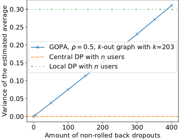
Figure 3: Impact of non-rolled back dropouts on the utility of Gopa. See text for details.

Figure 3 illustrates with a simple simulation the impact of a small number of residual pairwise noise terms of variance $\sigma_{\Delta}^{2}$ in the final result, which may happen in the rare circumstances that the pairwise noise terms of some users who dropped out are not “rolled back” by their neighbors (step 2 above). We consider $n=10000$, $\rho=0.5$, $\varepsilon=0.1$, $\delta=10/(\rho n)^{2}$, $\kappa=0.3$ and set the values of $k$, $\sigma^{2}_{\eta}$ and $\sigma^{2}_{\Delta}$ using Corollary 1 so that Gopa satisfies $(\varepsilon,\delta)$-DP (in particular we set them in the same way as in Table 2). We simulate this by drawing a random $k$-out graph, selecting a certain number of dropout users at random, marking all their exchanged noise as not rolled back (in practice its is also possible that part of their noise gets rolled back) and computing the variance of the estimated average. The simulation is averaged over $100$ runs (even though the standard deviation across random runs is negligible). We see that Gopa can tolerate a number of “catastrophic drop-outs” while remaining more accurate than local DP. This ability to retain a useful estimate despite residual pairwise noise terms is rather unique to Gopa, and not possible with secure aggregation methods which typically use uniformly random pairwise masks Bonawitz2017a . We note that this robustness can be optimized by choosing smaller $\sigma^{2}_{\Delta}$ (i.e., smaller $\kappa$) and compensating by adding a bit more independent noise according to Corollary 1.

B.3 Robustness Against Attacks on Efficiency

In this section, we study several attacks, their impact and Gopa’s defense against them.

Dropout

A malicious user could drop out of the computation intentionally, with the impact described in Section B.2. However, dropping out is bad for the reputation of a user, and users dropping out more often than agreed could be banned from future participation. One can use techniques from identity management (a separate branch in the field of security) to ensure that creating new accounts is not free, and that possibilities to create new accounts are limited, e.g., by requiring to link accounts to unique persons, unique bank account or similar. This also ensures that the risk of being banned outweighs the incentive of the (bounded) delay of the system one could cause by intentionally dropping out.

Flooding with Neighbor Requests

In Section 5, we discuss privacy guarantees for complete graphs, path graphs and random communication graphs. In the case of a complete communication graph, all users exchange noise with all other users. This is slow, but there is no opportunity for malicious users to interfere with the selection of neighbors as the set of neighbors is fixed. In other cases, e.g., when the number of users is too large and every user selects $k$ neighbors randomly as in Section 5.4, one could wonder whether colluding malicious users could select neighbors in such a way that the good working of the algorithm is disturbed, e.g., a single honest user is flooded with neighbor requests and ends up exchanging noise with $O(n)$ others.

We first stress the fact that detecting such attacks is easy. If all agents randomly select neighbors uniformly at random as they should, then every agent expects to receive $k$ neighbor invitations, perhaps plus a few standard deviations of order $O(\sqrt{k})$. As soon as a user receives a sufficiently unlikely number of neighbor invitations, we know that with overwhelming probability the user is targeted by malicious users.

To avoid this, we can let all users select neighbors in a deterministic way starting from a public random seed (e.g., take the public randomness generated in Section B.1, add the ID of the user to it, apply a hash function to the sum, and use the result to start selecting neighbors). In this way, neighbor selection is public and can’t be tampered with. It is possible some neighbors of a user $u$ were off-line and $u$ skipped them, but unless so many users are off-line that the community should have noticed severe problems $u$ should be able to find enough neighbors among the first $ck$ in his random sequence for a small constant $c$.

Other Common Attacks

We assume the algorithm is implemented on a system which is secure according to classic network-related attacks, such as denial-of-service (DoS) attacks. Such attacks are located at the network level rather than at the algorithm level. As such, they apply similarly to any distributed algorithm requiring communication over a network. To the extent such attacks can be mitigated, the solutions are on the network level, including (among others) a correct organization of the network and its routers.

Similarly, we assume that all (honest) communication is secure and properly encrypted, referring the reader to the state-of-the-art literature for details on possible implementations.

B.4 Further Discussion on the Impact of Finite Precision

In practice, we cannot work with real numbers but only with finite precision approximations, see Section 6.1. We provide a brief discussion of the impact of this on the guarantees offered by the protocol. There is already a large body of work addressing issues which could arise because of finite precision. Here are the main points:

1. Finite precision can be an issue for differential privacy in general, (see e.g. balcer_et_al:LIPIcs:2018:8353 for a study of the effect of floating point representations). Issues can be overcome with some care, and our additional encryption does not make the problem worse (in fact we can argue that encryption typically uses more bits and in our setting this may help).

2. The issue of finite precision has been studied in cryptography. While some operations such as multiplication can cause difficulties in the context of homomorphic encryption, in our work we use a partially homomorphic scheme with only addition. As a result, we can just represent our numbers with as many bits (after the decimal dot) as in plaintext memory.

3. If the number of users is high (and hence also the sum of the $X_{u}$ and the $\Delta_{u,v}$ variables), working up to the needed precision doesn’t cause a cost which is high compared to the cost of the digits before the decimal dot.

Appendix Appendix C Complexity of Gopa

The cost of the protocol in terms of computation and communication was summarized in Theorem 7.1. This section summarizes each component of this cost, relying in particular on the cost of proving computations in 6.

Dominant computations are exponentiations in the cryptographic group $\mathbb{G}$ defined in Section 6.1. The cost of signing messages is negligible. We describe costs centered on any user $u\in U$ . For simplicity, when we say a task costs $c$, it means that costs at most $c$ computations for proving a computation, $c$ computations for another party verifying this computation and it requires the exchange of $cW$ bits, where $W$ is the size in bits of an element of $\mathbb{G}$. Some computations depend on fixed-precision parameter ${\psi}$ to represent numbers in $\mathbb{Z}_{q}$ (see Section 6.1) and the amount $1/B$ of equiprobable bins used to sample independent noise $\eta_{u}$ (see Appendix D.4).

The costs break down as follows:

• The Phase 2 Setup requires generating public randomness which has constant cost (except for $O(1)$ parties that perform some extra computations, see Algorithm 3) and private seeds that require 2 range proofs in the interval $[0,1/B{\psi}]$, with a final cost of $20\log_{2}(1/B)+20\log_{2}(1/{\psi})$.

• Validity of input at Phase 3 Verification requires a range proof in the interval $[0,1/{\psi}]$, with a cost of $10\log_{2}(1/{\psi})$. Extra computations of consistency cannot be accounted here as they depend on the nature of external computations.

• Correctness of computations of properties (9) and (10) at Phase 3 Verification cost at most $5|N(u)|+4$, accounting the computations over commitments and proofs of knowledge of terms of each property.

• The verification of Property (11) at Phase 3 Verification costs $\ln(1/B)\cdot(34.1\ln(1/{\psi})+7.22\ln(q))$ (see Appendix D.4).

The overall cost of a protocol for user $u$ is at most of

$$5|N_{u}|+20\log_{2}(1/B)+30\log_{2}(1/{\psi})+\ln(1/B)\cdot(34.1\ln(1/{\psi})+7.22\ln(q))+4.$$

Supplementary Material

This supplementary materials file contains background, often a summary of what can be found elsewhere in literature, and further details, which are not essential for the elaboration of the contribution.

Appendix Appendix D Further Details on Cryptography and Security

D.1 Commitment Schemes

We start by defining formally a commitment and its properties.

Definition 2 (Commitment Scheme)

A commitment scheme consists of a pair of (computationally efficient) algorithms $(Setup,Com)$. The setup algorithm $Setup$ is executed once, with randomness $t$ as input, and outputs a tuple $\Theta\leftarrow Setup(t)$, which is called the set of parameters of the scheme. The algorithm $Com$ with parameters $\Theta$, denoted $Com_{\Theta}$, is a function ${Com_{\Theta}:\mathcal{M}_{\Theta}\times\mathcal{R}_{\Theta}\rightarrow\mathcal{C}_{\Theta}}$, where $\mathcal{M}_{\Theta}$ is called the message space, $\mathcal{R}_{\Theta}$ the randomness space, and $\mathcal{C}_{\Theta}$ the commitment space. For a message $m\in\mathcal{M}_{\Theta}$, the algorithm draws $r\in\mathcal{R}_{\Theta}$ uniformly at random and computes commitment $\mathbf{c}\leftarrow Com_{\Theta}(m,r)$.

The security of a commitment scheme typically depends on $t$ not being biased, in particular, it must be hard to guess non-trivial information about $t$.

We now define some key properties of commitments.

Property 1 (Hiding Property)

A commitment scheme is hiding if, for all secrets $x\in\mathcal{M}_{\Theta}$ and given that $r$ is chosen uniformly at random from $\mathcal{R}_{\Theta}$, the commitment $\mathbf{c_{x}}=Com_{\Theta}(x,r)$ does not reveal any information about $x$.

Property 2 (Binding Property)

A commitment is binding if there exists no computationally efficient algorithm $\mathcal{A}$ that can find $x_{1},x_{2}\in\mathcal{M}_{\Theta}$, $r_{1},r_{2}\in\mathcal{R}_{\Theta}$ such that $x_{1}\neq x_{2}$ and ${Com_{\Theta}(x_{1},r_{1})=Com_{\Theta}(x_{2},r_{2})}$.

Property 3 (Homomorphic Property)

A homomorphic commitment scheme is a commitment scheme such that $\mathcal{M}_{\Theta}$, $\mathcal{R}_{\Theta}$ and $\mathcal{C}_{\Theta}$ are abelian groups, and for all $x_{1},x_{2}\in\mathcal{M}_{\Theta}$, $r_{1},r_{2}\in\mathcal{R}_{\Theta}$ we have

$$Com_{\Theta}(x_{1},r_{1})+Com_{\Theta}(x_{2},r_{2})=Com_{\Theta}(x_{1}+x_{2},r_{1}+r_{2}).$$

Please note that the three occurrences of the ’$+$’ sign in the above definition are operations in three difference spaces, and hence may have different definitions and do not necessarily correspond to normal addition of numbers.

Pedersen Commitments

Let $p$ and $q$ be two large primes such that $q$ divides $p-1$, and a let $\mathbb{G}$ be cyclic subgroup of order $q$ of the multiplicative group $\mathbb{Z}^{*}_{p}$. For such group, we have that $\mathbb{G}=\{a^{i}\mod p\mid 0\leq i<q\}$ for any $a\in\mathbb{G}$ distinct to $1$. In the Pedersen scheme, $Setup$ is a function that samples at random parameters $\Theta=(\mathbb{G},g,h)$ where $g,h$ are two generators of $\mathbb{G}$ Additionally, $\mathcal{M}_{\Theta}=\mathcal{R}_{\Theta}=\mathbb{Z}_{q}$, and $\mathcal{C}_{\Theta}=\mathbb{G}$. We will refer to $g$ and $h$ as bases. The commitment function $Com_{\Theta}$ is defined as

$$Com_{\Theta} : \mathbb{Z}_{q}\times\mathbb{Z}_{q}\rightarrow\mathbb{G}$$

$$Com_{\Theta}(x,r) = g^{x}\cdot h^{r},$$ (38)

where $(\cdot)$ is the product modulo $p$ of group $\mathbb{G}$, $x$ is the secret and $r$ is the randomness. For simplification and when $r$ is not relevant, we relax the notation $Com_{\Theta}(x,r)$ to $Com_{\Theta}(x)$ and assume $r$ is drawn appropriately. Pedersen commitments are homomorphic (in particular, $Com_{\Theta}(x+y,r+s)=Com_{\Theta}(x,r)\cdot Com_{\Theta}(y,s)$), unconditionally hiding, and computationally binding under the Discrete Logarithm Assumption, which we succinctly describe below. For more details, see Chapter 7 of katz_introduction_2014 .

Assumption 1 (Discrete Logarithm Assumption)

Let $\mathbb{G}$ be a cyclic multiplicative group of large prime order $q$, and $g$ and $h$ two elements chosen independently and uniformly at random from $\mathbb{G}$. Then, there exists no probabilistic polynomial time algorithm $\mathcal{A}$ that takes as input the tuple $(\mathbb{G},q,g,h)$ and outputs a value $b$ such that $P(g^{b}=h)$ is significant on the size of $q$.

An optimized implementation of Pedersen commitments can be found in franck_efficient_2017 . To generate a common Pedersen scheme in our adversary model, the generation of the unbiased random input $t$ for $Setup$ can be done as described in Algorithm 3 of Appendix D.3.

D.2 Zero Knowledge Proofs

Zero Knowledge Proofs (ZKP) goldwasser_knowledge_1989 allow to prove statements about private committed values. We use $\Sigma$-protocols cramer_modular_1997 , a type of ZKP which can prove arithmetic relations, range membership and certain types of logical formulas. We explain basic concepts about ZKP in Section D.2.1 and $\Sigma$-protocols in Section D.2.2.

D.2.1 Zero Knowledge Proofs and Arguments

ZKP are a special case of interactive Proofs of Knowledge (PoK). We first define PoK. For a NP relation $\mathcal{R}$, a PoK is a protocol between a prover $\mathcal{P}$ and a verifier $\mathcal{V}$ in which $\mathcal{P}$ tries to prove to $\mathcal{V}$ that he knows a witness $w$ such that $(a,w)\in\mathcal{R}$ for a public statement $a$. At the end of the protocol, $\mathcal{V}$ either accepts or rejects the proof. We denote by $(a;w)$ to a member of a relation or an input of a protocol, using a semicolon to separate the public statement $a$ from the private witness $w$. The tuple of all messages in a proof is called the conversation or transcript. A ZKP is a PoK that satisfy the following properties:

• Completeness: a proof is complete if $\mathcal{V}$ always accepts the proof when $(a;w)\in\mathcal{R}$ and $\mathcal{P}$ knows $w$.

• Soundness: a proof is sound if any prover whose proof for statement $a$ is accepted by the verifier knows a valid witness $w$ such that $(a;w)\in\mathcal{R}$ with overwhelming probability. The notion of soundness we use is called witness extended emulation lindell_parallel_2003 . Proofs that are sound only if the prover is computationally bounded are also called arguments.

• Zero Knowledge: a proof is zero knowledge if its transcript reveals no or negligible information about the witness other than its validity.

D.2.2 $\Sigma$-Protocols

Here we explain the basics to understand classic $\Sigma$-protocols proposed by cramer_modular_1997 ; cramer_zero-knowledge_1998 . While the proofs defined therein are applicable for a wide family of commitments, we instantiate them for the Pedersen scheme.

A $\Sigma$-protocol is a 3-message PoK with a transcript of the form $(m_{1},t,m_{2})$, where $m_{1}$ and $m_{2}$ are messages of $\mathcal{P}$, and $t$ is a message of $\mathcal{V}$ called challenge, which is uniformly distributed in some challenge space $S$. The size of $S$ is linear in $q$ (see Appendix D.1).

The security of these protocols rely on $\mathcal{V}$ behaving honestly in the draw of challenges. To circumvent this in settings where no trusted verifier is available, $\Sigma$-protocols can be transformed to non-interactive using the Fiat-Shamir heuristic fiat_how_1987 ; bernhard_how_2012 . This consists on replacing the challenge of $\mathcal{V}$ by a hash function that computes $t$ from $m_{1}$ and the statement of the proof. Then, a prover can generate a transcript by itself and send it to an untrusted verifier. This transformation is proven secure when the hash function is modeled as a random oracle bellare_random_1993 . We will use this transformation for both classic and compressed $\Sigma$-protocols described in the following sections. However, for simplicity, we will describe protocols in their interactive form.

Below, we describe some existent protocols, explain their complexity and refer to the literature for other aspects such as security proofs. The protocols are secure under the DLA and instantiated for Pedersen commitments, described in Appendix D.1. Recall parameters $\mathbb{Z}^{*}_{p}$, $\mathbb{Z}_{q}$, $\mathbb{G}$, $g$ and $h$ defined therein. For some building blocks, we use extra pairs of elements of $\mathbb{G}$ as bases of for $\Theta$, where bases belonging to the same pair are always assumed to be chosen independently at random from $\mathbb{G}$. Recall that $p$ is the order of $\mathbb{Z}^{*}_{p}$, of which $\mathbb{G}$ is subgroup of. Products and exponentiations of members of $\mathbb{G}$ are group operations, which means that they are implicitly modulo $p$. To analyze the computational cost of the building blocks, we count group exponentiations (GEX), which are the dominant operations. For a ZKP, we call the size of a proof to the size of the transcript. To describe sizes of proofs, we use $W$ for the size in bits of an element of $\mathbb{G}$. In that context, $W$ is equal to $\lfloor\log_{2}p\rfloor+1$, but in some implementations the size can be different so we abstract from details. $a\leftarrow_{R}S$ means that $a$ is sampled uniformly at random from elements of $S$.

Basic proof of knowledge

This proof is also known as the basic protocol. It allows $\mathcal{P}$ to prove that he knows an opening of a commitment $P$. That is, a value $x$ and randomness $r$ such that $P=g^{x}h^{r}$. This is a proof for the relation

$$\{(P\in\mathbb{G};x,r\in\mathbb{Z}_{q}):P=g^{x}h^{r}\}.$$

The protocol goes as follows:

1. $\mathcal{P}$ draws $a,b\leftarrow_{R}\mathbb{Z}_{q}$, computes $A\leftarrow g^{a}h^{b}$ and sends $A$ to $\mathcal{V}$.

2. $\mathcal{V}$ draws a challenge $t\leftarrow_{R}\mathbb{Z}_{q}$ and sends it to $\mathcal{P}$.

3. $\mathcal{P}$ computes $d\leftarrow a+xt\pmod{q}$ and $e\leftarrow b+rt\pmod{q}$ and sends $(d,e)$ to $\mathcal{V}$.

4. $\mathcal{V}$: if $g^{d}h^{e}=AP^{t}$ then accept, else reject

The computational cost of the proof is $2$ GEX for $\mathcal{P}$, and $3$ for $\mathcal{V}$. The proof size is of $3W$ bits. This protocol was first proposed by schnorr_efficient_1991 for a single base, and adapted to many bases (in our case, $g$ and $h$) in chaum_improved_1988 .

We provide an intuition of how ZKP properties are obtained for the basic proof of knowledge. Completeness follows directly from the homomorphic property. For soundness, consider a prover $\mathcal{P}^{*}$ that, by following the protocol, can produce an accepting transcript $(A,t_{1},(d_{1},e_{1}))$ with significant probability. Then it is shown that also with non-negligible probability, by using $\mathcal{P}^{*}$’s strategy many times, another accepting transcript of the form $(A,t_{2},(d_{2},e_{2}))$ can be produced, where the first message is equal in both transcripts and such that $t_{1}\neq t_{2}$. Now, since both transcripts are accepting, we have $g^{d_{1}}h^{e_{1}}=AP^{t_{1}}$ and $g^{d_{2}}h^{e_{2}}=AP^{t_{2}}$ so $\mathcal{P}^{*}$ can efficiently compute the witness $x=\frac{d_{1}-d_{2}}{t_{1}-t_{2}}$ and $r=\frac{e_{1}-e_{2}}{t_{1}-t_{2}}$ which is valid as $g^{x}h^{r}=P$. Either $\mathcal{P}^{*}$ already knew it or he can efficiently compute the discrete logarithms base $g$ of $h$, which is a contradiction due to the DLA.

Zero knowledge is obtained by showing that all information seen in the proof is randomness that does not depend on the secrets. By only knowing the statement $P$ one can sample $d^{\prime}\leftarrow_{R}\mathbb{Z}_{q}$, $e^{\prime}\leftarrow_{R}\mathbb{Z}_{q}$ and $t^{\prime}\leftarrow_{R}\mathbb{Z}_{q}$, compute $A^{\prime}=P^{-t^{\prime}}g^{d^{\prime}}h^{e^{\prime}}$ and generate the transcript $(A^{\prime},t^{\prime},(d^{\prime},e^{\prime}))$ has the same distribution as a conversation between an honest prover and an honest verifier. Note that, as it is computed in reverse, $(A^{\prime},t^{\prime},(d^{\prime},e^{\prime}))$ cannot be efficiently produced by a dishonest prover in the actual protocol, as the order of messages cannot be changed.

In the following, we will present $\Sigma$-protocols that use similar arguments as the ones described for the basic proof of knowledge to prove their properties. In particular, they can all generate accepting transcripts “in reverse” even if witnesses are not known, as shown to prove the zero knowledge property above. We will not describe their security proofs, but we will point to the literature where these can be found.

Proof of equality

This proof allows $\mathcal{P}$ to prove that he committed to the same private value $x$ in two different commitments $P=g_{1}^{x}h_{1}^{r}$ and $P^{\prime}=g_{2}^{x}h_{2}^{r^{\prime}}$. That is, the relation

$$\{(P,P^{\prime}\in\mathbb{G};x,r,r^{\prime}\in\mathbb{Z}_{q}):P=g_{1}^{x}h_{1}^{r}\land P^{\prime}=g_{2}^{x}h_{2}^{r^{\prime}}\}.$$

The pairs of bases $(g_{1},h_{1})$ and $(g_{2},h_{2})$ might be different. This proof is described by chaum_wallet_1993 for a single base and a generalization for many bases can be found in chaum_improved_1988 . The protocol goes as follows:

1. $\mathcal{P}$ generates $a,b,c\leftarrow_{R}\mathbb{Z}_{q}$, computes $A\leftarrow g_{1}^{a}h_{1}^{b}$ and $B\leftarrow g_{2}^{a}h_{2}^{c}$ and sends $(A,B)$ to $\mathcal{V}$.

2. $\mathcal{V}$ draws a challenge $t\leftarrow_{R}\mathbb{Z}_{q}$ and sends it to $\mathcal{P}$.

3. $\mathcal{P}$ computes $d\leftarrow a+xt\pmod{q}$, $e\leftarrow b+rt\pmod{q}$ and $f\leftarrow c+r^{\prime}t\pmod{q}$ and sends $(d,e,f)$ to $\mathcal{V}$.

4. $\mathcal{V}$: if $g_{1}^{d}h_{1}^{e}=AP^{t}$ and $g_{2}^{d}h_{2}^{f}=B(P^{\prime})^{t}$, then accept else reject.

The proof requires the computation of $4$ GEX for $\mathcal{P}$ and $6$ for $\mathcal{V}$. The proof size is of $5W$ bits.

Composition

Let $\Pi_{1}$ and $\Pi_{2}$ be two $\Sigma$-protocols for ZKP of relations $\mathcal{R}_{1}$ and $\mathcal{R}_{2}$ respectively. A single $\Sigma$-protocol to prove the relation

$$\mathcal{R}_{\land}=\{(a,a^{\prime};w,w^{\prime}):(a;w)\in\mathcal{R}_{1}\land(a^{\prime};w^{\prime})\in\mathcal{R}_{2}\}$$

can be easily constructed. Basically, we just make both proofs to share the same challenge. The protocol is as follows. The first message is $(m_{1},m_{1}^{\prime})$, where $m_{1}$ and $m_{1}^{\prime}$ are exactly as generated for the first messages of $\Pi_{1}$ and $\Pi_{2}$ respectively. Then $\mathcal{V}$ generates the challenge $t$ and sends it to $\mathcal{P}$. Next, $\mathcal{P}$ generates the third message $(m_{2},m_{2}^{\prime})$ where $m_{2}$ and $m_{2}^{\prime}$ are generated from $(m_{1},t)$ and from $(m_{1}^{\prime},t)$ as they will be generated for the third messages of $\Pi_{1}$ and $\Pi_{2}$ respectively. Finally $\mathcal{V}$ verifies $(m_{1},t,m_{2})$ and $(m_{1}^{\prime},t,m_{2}^{\prime})$ are accepting as in $\Pi_{1}$ and $\Pi_{2}$. Using this composition, if we wish to prove statements over many relations, we can do it with a single $\Sigma$-protocol.

Another technique allows to construct ZKPs of disjunctions of statements. The work by cramer_proofs_1994 proposed a $\Sigma$-protocol for the relation

$$\mathcal{R}_{\lor}=\{(a,a^{\prime};w,w^{\prime}):(a;w)\in\mathcal{R}_{1}\lor(a^{\prime};w^{\prime})\in\mathcal{R}_{2}\},$$

where $\Pi_{1},\Pi_{2},\mathcal{R}_{1}$ and $\mathcal{R}_{2}$ are defined as for conjunctions. We briefly describe the protocol below. Without loss of generality, assume that $\mathcal{P}$ knows $(a;w)\in\mathcal{R}_{1}$, but he does not know $(a^{\prime};w^{\prime})\in\mathcal{R}_{2}$ and that $\mathcal{V}$ does not know which of the two witnesses is known by $\mathcal{P}$. As $\Pi_{2}$ is zero knowledge, an accepting transcript $(m_{1}^{\prime},t_{b},m_{2}^{\prime})$ can be generated in reverse as shown for the proof of knowledge above and without $\mathcal{P}$ knowing a valid witness.

1. $\mathcal{P}$ generates $(m_{1}^{\prime},t_{b},m_{2}^{\prime})$ in reverse and generates $m_{1}$ as he would normally do for the first message of $\Pi_{1}$.

2. $\mathcal{P}$ sends $(m_{1},m_{1}^{\prime})$ to $\mathcal{V}$.

3. $\mathcal{V}$ draws a challenge $t\leftarrow_{R}\mathbb{Z}_{q}$ and sends it to $\mathcal{P}$.

4. $\mathcal{P}$ computes $t_{a}\leftarrow t-t_{b}\bmod q$ and computes $m_{2}$ from $m_{1}$ and $t_{a}$ as he would have done in the original protocol $\Pi_{1}$.

5. $\mathcal{P}$ sends $(m_{2},m_{2}^{\prime})$ to $\mathcal{V}$.

6. $\mathcal{V}$ checks that $(m_{1},t_{a},m_{2})$ and $(m_{1}^{\prime},t_{b},m_{2}^{\prime})$ are accepting as in protocols $\Pi_{1}$ and $\Pi_{2}$, and that $t_{a}+t_{b}\bmod q$ is equal to $t$. If all checks pass, then accept. Otherwise reject.

Here, $\mathcal{P}$ can generate $(m_{1},t_{a},m_{2})$ as he knows a witness for $\mathcal{R}_{1}$ and he can simulate an accepting transcript for $\mathcal{R}_{2}$. As $t_{a}+t_{b}\bmod q=t$, $\mathcal{V}$ is ensured that at least either $t_{a}$ or $t_{b}$ is unpredictable for $\mathcal{P}$ when generating the first message of the proof, so he would not be able to pass the proof with significant probability unless he knows at least one witness. We refer to the paper for the security proofs and further details.

The composition techniques outlined above allow one to prove logical formulas of conjunctions and disjunctions of statements. The computational and communication cost for the resulting protocol is similar to the sum of the costs of the proof of each composed statement.

Proof of linear relation

Let $\bar{x}=(x_{i})_{i=1}^{k}$ for some $k>0$ be a vector of private values, $\bar{P}=(P_{i})_{i=1}^{k}$ a public vector of commitments such that $P_{i}$ is a commitment of $x_{i}$, $\bar{a}=(a_{i})_{i=1}^{k}$ a public vector of integer coefficients, and $b$ a public scalar. The goal of $\mathcal{P}$ is to prove the equality $\langle\bar{x},\bar{a}\rangle=b\pmod{q}$, where $\langle\cdot,\cdot\rangle$ is the inner product. The proof follows almost directly from the homomorphic property of commitments. We have that $P_{L}=\prod_{i=1}^{k}P_{i}^{a_{i}}$ is a valid commitment of $\langle\bar{x},\bar{a}\rangle$. Then, $\mathcal{P}$ and $\mathcal{V}$ prove that values committed with $P_{L}$ and $P_{b}=g^{b}$ are equal. Note that it is not necessary to use the base $h$ to compute the commitment $P_{b}$ as $b$ is publicly known and hence we can use randomness equal to $0$. The proven relation is

$$\Big{\{}(\bar{P}\in\mathbb{G}^{k},\bar{a}\in\mathbb{Z}_{q}^{k},b\in\mathbb{Z}_{q};\bar{x},\bar{r}=(r_{i})_{i=1}^{k}\in\mathbb{G}^{k})$$

$$:\bigwedge_{i=1}^{k}P_{i}=g^{x_{i}}h^{r_{i}}\land\langle\bar{a},\bar{x}\rangle=b\pmod{q}\Big{\}}.$$

where $\bar{r}$ is the randomness for each commitment. For $\mathcal{P}$ and $\mathcal{V}$, the proof requires $k+1$ GEX to compute $P_{L}$ and $P_{b}$ plus one proof of equality. This leads to a final cost of $k+5$ GEX for $\mathcal{P}$ and $k+7$ for $\mathcal{V}$. Considering that initial commitments $\bar{P}$ are already shared with $\mathcal{V}$ and that $\mathcal{P}$ has already proven knowledge of them, the proof size is equal to that of the proof of equality, which is $5W$ bits.

Proof of a committed bit

A handy special case of the composition using disjunction is a proof that a secret $b$ is a bit, i.e. that $\{b=0\lor b=1\}$. This instantiation is described by (mao_guaranteed_1998 Section 3.2 therein). It requires $3$ GEX for $\mathcal{P}$ and $4$ for $\mathcal{V}$. The size of the proof is of $4W$ bits.

Range proof

Here, the statement to prove is that, for a positive integer $M<q-1$ of $B_{M}$ bits and a commitment $P$, $\mathcal{P}$ knows an opening $x$ of $P$ that lies in the range $[0,M]$. This is a folklore proof that can be done by committing to the bits $b_{1},\ldots,b_{B_{M}}$ of the bit representation of $x$, i.e. that $x=\sum_{i=1}^{B_{M}}2^{i-1}b_{i}$. For $i\in\{1,\dots,B_{M}\}$ it is proven that $b_{i}$ is a bit with the protocol mentioned above. The validity of the decomposition of $x$ can be proven by a linear proof. This implies that $x\in[0,2^{B_{M}}-1]$. For ranges whose upper bound is not of the form $2^{B_{M}}-1$, $\mathcal{P}$ commits to $M-x$ and proves that it also lies in $[0,2^{B_{M}}-1]$. This finishes the proof for arbitrary ranges.

Committing to every bit $b_{i}$ has a cost of $B_{M}$ GEX for $\mathcal{P}$. The cost of proofs of bits is dominated by $3B_{M}$ GEX for $\mathcal{P}$ and $4B_{M}$ for $\mathcal{V}$. The proof that these bits are the decomposition of $x$ is dominated by $B_{M}$ GEX for both $\mathcal{P}$ and $\mathcal{V}$. For arbitrary ranges, the cost duplicates as described above. The total cost of the proof is dominated by $10\log_{2}(M)$ GEX for $\mathcal{P}$ and the same cost for $\mathcal{V}$. The size of the proof is dominated by $10\log_{2}(M)W$ bits.

Proof of product

In this proof, $\mathcal{P}$ wants to prove the knowledge of openings $a$, $b$ and $d$ of commitments $P_{a}=g^{a}h^{r_{1}}$, $P_{b}=g^{b}h^{r_{2}}$ and $P_{d}=g^{d}h^{r_{3}}$ and that they satisfy $ab=d\pmod{q}$. This proof can be done in a straightforward way with the knowledge and equality proofs. We use the fact that, by properties of our cyclic group $\mathbb{G}$, $P_{a}$ is not only a commitment but also a base, and that $P_{d}=(P_{a})^{b}h^{(r_{3}-br_{1})}$ is a valid commitment for $b$ using bases $(P_{a},h)$. For the proof, $\mathcal{P}$ first proves the knowledge of an opening of $P_{a}$, and then it proves the equality of two openings $P_{b}$ and $P_{d}$ with the proof of equality, where commitments are computed with the pairs of bases $(g,h)$ and $(P_{a},h)$ respectively. If $\mathcal{P}$ does not know the commitment of a product of $ab$ hidden in $P_{d}$ it would not pass the proof. The proof is the instantiation for Pedersen commitments of the protocol by cramer_zero-knowledge_1998 , and requires $6$ GEX for $\mathcal{P}$ and $9$ for $\mathcal{V}$. The proof size is of $8W$ bits.

Proof of modular sum

Here, $\mathcal{P}$ wants to prove that, for a public modulus $M<q/2$, a public value $t\in[0,M-1]$ and two secrets $x,z\in[0,M-1]$, the relation $x=z+t\mod M$ is satisfied. Let $P_{x}$ and $P_{z}$ be the commitments of $x$ and $z$ respectively. First, $\mathcal{P}$ does two range proofs to prove that $x$ and $z$ lie in $[0,M-1]$. Then it proves that an auxiliary value $b$ is a bit. Finally it proves that ${x=z+t-bM\pmod{q}}$ with a linear proof. Because of their range, we have that $z+t<q$, hence the modulus $q$ does not interfere and the linear equality holds if and only if the modular sum is satisfied. This proof is inspired by the more general proof of modular sum proposed by camenisch_proving_1999 . Its complexity is given by the composition of the proofs mentioned above, where the dominant term comes from the two range proofs, and amounts to $20\log_{2}(M)$ GEX for $\mathcal{P}$ and the same for $\mathcal{V}$. The size of the proof is of $20\log_{2}(M)W$ bits.

D.3 Public Randomness

We provide here an algorithm to generate public randomness which, compared to the sketch provided in Section B.1, distributes the cost more evenly over the participants. In particular, we provide a decentralized method to generate $n$ public random numbers in $\mathbb{Z}_{q}$ with a computational effort of $O(1)$ per user, and costs logarithmic in $n$ for a negligible portion of users. In Gopa it is used among others to generate private random seeds and to initialize the Pedersen commitment parameters $\Theta$ shared by all users.

In our procedure, we enumerate users from $1$ to $n=|U|$ and use the cryptographic hash function $H$ described at the beginning of the Section to generate random numbers over $\mathbb{Z}_{2^{T}}$. We also make use of a commitment function $Com$, for which a common trusted initialization is not required (see for example blum_coin_1983 ). The procedure is depicted in Algorithm 3.

Algorithm 3 Generation of Public Randomness

1:  Input: Hash function $H$ and a commitment function $Com$.

2:  for all $u\in\{1,\dots,n\}$  do

3:     Draw ${s_{u}\leftarrow_{R}\mathbb{Z}_{q}}$, compute ${\mathbf{c_{u}}\leftarrow Com(s_{u})}$ and publish $\mathbf{c_{u}}$

4:  end for

5:  for all $u\in\{1,\dots,n\}$  do

6:      Set $s[u,u]\leftarrow s_{u}$ and publish it

7:  end for

8:  for $j=1$ to $\lfloor\log_{2}(n)\rfloor+1$ sequentially  do

9:     for all $i\in\{0,\dots,\lfloor n/2^{j}\rfloor\}$  do

10:         Let $u_{min}=2^{j}i+1$ and $u_{max}=\min(2^{j}(i+1),n)$

11:        if $s[u_{min},u_{max}]$ is not already published then

12:           Let $u_{mid}=u_{min}+2^{j-1}-1$

13:           A user $u\in\{u_{min},\dots,u_{max}\}$ wakes up and:

14:           $\bullet$ queries $(s[u_{min},u_{mid}]$, $s[u_{mid}+1,u_{max}])$, if a value is not published, set it to $0$

15:            $\bullet$ publishes ${s[u_{min},u_{max}]\leftarrow s[u_{min},u_{mid}]+[u_{mid}+1,u_{max}]}\mod q$

16:        end if

17:     end for

18:  end for

19:  for all  $u\in\{1,\dots,n\}$  do

20:      Query $S\leftarrow s[1,n]$ and publish $t_{u}\leftarrow H(S+u)$

21:  end for

22:   Output: A set of unbiased random numbers $t_{1},\dots,t_{n}\in\mathbb{Z}_{2^{T}}$

The “commit-then-reveal” protocol from in lines 2-6 is to avoid users from choosing the value $s_{u}$ depending on the choice of other users, which could bias the final seed $S=\sum_{u\in U}s_{u}\mod q$. The value $S$, computed in lines 8-15 in a distributed way, requires at most $O(\log(n))$ queries and sums for a user in the worst case, but $O(1)$ for almost all users. Inactive users do not affect the computation, but their $s_{u}$ terms might be ignored. As it is computed from modular sums, $S$ is uniformly distributed over $\mathbb{Z}_{q}$ if at least one active user is honest. Finally, we compute our public random numbers $t_{1},\dots,t_{n}$ in lines 19 and 20, which are unpredictable due to the properties of $H$ and the unpredictability and uniqueness of its input $S+u$.

To verify that a user $u$ participated correctly, one needs to check that (1) the commitment $\mathbf{c_{u}}$ was properly computed from $s_{u}$, (2) all sums $s[u_{min},u_{max}]$ that $u$ published were computed correctly, and (3) the challenge $t_{u}$ was correctly computed from $S+u$ by the application of $H$.

The cost of the protocol for a user is dominated in the worst case at by $\log_{2}(n)$ sums and $3\log_{2}(n)W$ bits in total, corresponding to the several queries of $s[u_{min},u_{mid}]$ and $s[u_{mid}+1,u_{max}]$ and the publication of its sum. However, this is cost applies to only $O(1)$ users, while the rest of the users computes one commitment, one evaluation of $H$ and $O(1)$ sums and transfers $O(1)$ bits during the execution.

D.4 Private Gaussian Sampling

In our algorithm, every user $u$ needs to generate a Gaussian distributed number $\eta_{u}$, which he does not publish, but for which we need to verify that it is generated correctly, as otherwise a malicious user could bias the result of the algorithm.

Proving the generation of a Gaussian distributed random number is more involved than ZKPs such as linear relationships and range proofs we need to verify in the other parts of the computation.

Recall that $\psi$ is the desired fixed precision and $B$ is a precision parameter such that $B^{2}/\psi$ is an integer. We want to draw $\eta_{u}$ from the Gaussian distribution approximated with $1/B$ equiprobable bins and we want to prove the correct drawing up to a precision $B$.

We will start from the private seed $r_{u}$, generated in the Phase 2 Setup (Section B.1), which is only known to user $u$, for which $u$ has published a commitment $Com_{\Theta}(r_{u})$ and for which the other users know it has been generated uniformly randomly from an interval $[0,M-1]$ for $M\approx 1/B$. There are many ways now to exploit a uniformly distributed number to generate a Gaussian distributed one, but studying and comparing their efficiency and numerical quality is out of the scope of the current paper. Here, we only describe one strategy.

User $u$ will compute $x^{\prime}$ such that $((2r_{u}+1)/M)-1=\hbox{erf}(x^{\prime}/\sqrt{2})$. We know that $x^{\prime}$ is normally distributed. The main task is then to provide a ZKP that $y=\hbox{erf}(x)$ for $y=((2r_{u}+1)/M)-1$ and $x=x^{\prime}/\sqrt{2}$. As erf is symmetric, we do our analysis for positive values of $x$ and $y$, while the extension for the negative case is straightforward. We want to achieve an approximation where the error on $y$ as a function of $x$ is at most $B$.

Approximating the error function.

The error function relates its input and output in a way that cannot be expressed with additive, multiplicative or exponential equations. We therefore approximate erf using a converging series. In particular, we will rely on the series

$$\hbox{erf}(x)=\frac{2}{\sqrt{\pi}}\sum_{l=0}^{\infty}\frac{(-1)^{l}x^{2l+1}}{l!(2l+1)}.$$ (39)

As argued by chevillard:inria-00261360 , this series has two major advantages. First, it only involves additions and multiplications, while other known series converging to $\hbox{erf}(x)$ often include multiple $\exp(-x^{2}/2)$ factors which would require additional evaluations and proofs. Second, it is an alternating series, which means we can determine more easily in advance how many terms we need to evaluate to achieve a given precision.

Nevertheless, Equation (39) converges slowly for large $x$. It is more efficient to prove either that

$$y=\hbox{erf}(x)\quad or\quad 1-y=\hbox{erfc}(x),$$

as for $\hbox{erfc}(x)=1-\hbox{erf}(x)$ there exist good approximations requiring only a few terms for large $x$. An example is the asymptotic expansion

$$\hbox{erfc}(x)=\frac{e^{-x^{2}}}{x\sqrt{\pi}}S_{\mathrm{erfc}}(x)+R_{L}(x),$$ (40)

where

$$S_{\mathrm{erfc}}(x)=\sum_{l=0}^{L-1}\frac{(-1)^{l}(2l-1)!!}{(2x^{2})^{l}}$$ (41)

with $l!!=1$ for $l<1$ and $(2l-1)!!=\prod_{i=1}^{l}(2i-1)$. This series diverges, but if $x$ is sufficiently large then the remainder

$$R_{L}(x)\leq\frac{e^{-x^{2}}}{x\sqrt{\pi}}\frac{(2L-1)!!}{(2x^{2})^{L}}$$ (42)

after the first $L$ terms is sufficiently small to be neglected. So $u$ could prove either part of the disjunction depending on whether the erf or erfc approximations achieve sufficient precision.

Zero Knowledge Proof of $\hbox{erf}(x)$.

We consider use fixed-precision rounding operations. The implied rounding does not cause major problems for several reasons. First, the Gaussian distribution is symmetric, and hence the probability of rounding up and rounding down is exactly the same, making the rounding error a zero-mean random variable. Second, discrete approximations of the Gaussian mechanism such as binomial mechanisms have been studied and found to give similar guarantees as the Gaussian mechanism cp-sgd . Third, we can require the cumulated rounding error to be an order of magnitude smaller than the standard deviation of the noise we are generating, so that any deviation due to rounding has negligible impact. We will use a fixed precision for all numbers (except for small integer constants), and we will represent numbers as multiples of ${\psi}$.

Let $t_{l}=\frac{x^{2l+1}}{l!}$, and $L_{\mathrm{erf}}+1$ be the amount of terms of the series in Equation (39) we evaluate. We provide a ZKP of the evaluation of erf by proving that $t_{0}=x$,

$$t_{l} =\frac{t_{l-1}x^{2}}{l}\text{\quad}\text{for all }l\in\{1,\dots,L_{\mathrm{erf}}\},$$ (43)

and $y=\frac{2}{\sqrt{\pi}}\sum_{l=0}^{L_{\mathrm{erf}}}(-1)^{l}\frac{t_{l}}{2l+1}$. The bulk of the ZKP is in Equation (43) and in the divisions by $2l+1$ of the latter relation. For any fixed-precision value $d$, let $\langle d\rangle=\frac{d}{{\psi}}$ be its integer encoding. We can achieve a ZKP of the fixed precision product $c=ab$ for private $a$, $b$ and $c$ by proving that $\frac{1}{{\psi}}\langle c\rangle-\langle a\rangle\langle b\rangle\in[-1/2{\psi},1/2{\psi}]$. For round-off division, a ZKP that $a/b=c$ for private $a,c$ and a public positive integer $b$ is possible by proving that $\langle a\rangle-b\langle c\rangle\in[-b/2,b/2]$. The above proofs can be achieved using circuit and range proofs in $\mathbb{Z}_{q}$.

Similarly for erfc, let $m_{l}=(2l-1)!!/(2x)^{l}$ and $L_{\mathrm{erfc}}$ be the amount of terms we compute of the series defined in Equation (41), we can construct a ZKP of its evaluation by proving $m_{0}=0$,

$$m_{l}=m_{l-1}\frac{2l-1}{2x^{2}}\text{\qquad, for all }l\in\{1,\dots,L_{\mathrm{erfc}}-1\}$$ (44)

and $y=\frac{e^{-x^{2}}}{x\sqrt{\pi}}\sum_{l=0}^{L_{\mathrm{erfc}}-1}(-1)^{l}m_{l}.$ Proving that $\langle m_{l}\rangle\langle x^{2}\rangle-\frac{2l-1}{{\psi}}\langle m_{l-1}\rangle\in\left[-\langle x^{2}\rangle,\langle x^{2}\rangle\right]$ is equivalent to prove the relation in Equation (44). This can be done with $10B_{x^{2}}$ cost, where $B_{x^{2}}$ is maximum number of bits of $\langle x^{2}\rangle$. We can assume that $B_{x^{2}}\leq\log_{2}(q)$ (where $q$ is the order of the Pedersen group $\mathbb{G}$) which makes the cost for each term not bigger than $10\log_{2}(q)$. All other non-dominant computations can similarly be proven with circuit proofs.

To approximate the $\exp(-x^{2})$ term, the common series $\exp(z)=\sum_{i=0}^{\infty}z^{i}/i!$ is known to converge quickly. Even if its terms first go up until $z<i$, for larger $z$ where this could slow down convergence one can simply divide $z$ by a constant $a$ (maybe conveniently a power of $2$), approximate $\exp(z/a)$ and then compute $(\exp(z/a))^{a}$, which can be done efficiently. For simplicity, we omit the details here.

Amount of approximation terms.

Now we determine the magnitudes of $L_{\mathrm{erf}}$ and $L_{\mathrm{erfc}}$ needed to achieve an error smaller than $B$ in our computation. We then require the approximation and rounding error to be smaller than $B/2$. The amount of terms of the series must not depend on $x$ as the latter is a private value, but we must be able to achieve the expected precision for all possible $x$.

The erf series requires more approximation terms as $x$ gets larger. On the other hand, the erfc series is optimal when $L_{\mathrm{erfc}}=\lfloor x^{2}+1/2\rfloor$ terms are evaluated, and the error gets smaller as $x$ increases. Then, we use erfc only when $x$ is large enough to satisfy the required precision, and use erf for smaller values. We first compute the lower bound $x_{\mathrm{erfc}}^{min}$ for the application of erfc. Then the domain of erf is restricted to $\left[0,x_{\mathrm{erfc}}^{min}\right)$ so can obtain the an upper bound of $L_{\mathrm{erf}}$. Similarly, the restricted domain of erfc allows us to upper bound $L_{\mathrm{erfc}}$.

Developing Equation (42), we can achieve an approximation error of erfc of

$$E_{\mathrm{erfc}}(x) \leq \frac{1}{e^{x^{2}}x\sqrt{\pi}}\frac{(2L-1)!!}{(2x^{2})^{L}}=\frac{1}{e^{x^{2}}x\sqrt{\pi}}\frac{(2L)!}{L!2^{L}(2x^{2})^{L}}$$

$$\approx \frac{1}{e^{x^{2}}x\sqrt{\pi}}\frac{\sqrt{4\pi L}(2L/e)^{2L}}{\sqrt{2\pi L}(L/e)^{L}2^{L}(2x^{2})^{L}}=\frac{\sqrt{2}}{e^{x^{2}}x\sqrt{\pi}}\frac{(2^{2L})(L^{2L})(e^{L})}{(e^{2L})(L^{L})(2^{L})(2x^{2})^{L}}$$

$$= \frac{\sqrt{2}}{e^{x^{2}}x\sqrt{\pi}}\frac{2^{L}L^{L}}{e^{L}(2x^{2})^{L}}=\frac{\sqrt{2}}{e^{x^{2}}x\sqrt{\pi}}\frac{L^{L}}{e^{L}(x^{2})^{L}}.$$

This is minimal in $\lfloor x^{2}+1/2\rfloor$ so given $x$ we can achieve an error of

$$\frac{\sqrt{2}}{e^{x^{2}}x\sqrt{\pi}}\frac{L^{L}}{e^{L}(x^{2})^{L}} \leq \frac{\sqrt{2}}{e^{x^{2}}x\sqrt{\pi}}\frac{{\lfloor x^{2}+1/2\rfloor}^{\lfloor x^{2}+1/2\rfloor}}{e^{\lfloor x^{2}+1/2\rfloor}(x^{2})^{\lfloor x^{2}+1/2\rfloor}}\leq\frac{\sqrt{2}}{\sqrt{\pi}}\frac{(1+1/2x^{2})^{\lfloor x^{2}+1/2\rfloor}}{xe^{(2x^{2}-1/2)}}.$$

As we use erfc for large values of $x$, we assume $x\geq 1$ which will not affect our reasoning, then and we can simplify the above by

$$E_{\mathrm{erfc}}(x) \leq \frac{\sqrt{2}}{\sqrt{\pi}}\frac{(1+1/2x^{2})^{\lfloor x^{2}+1/2\rfloor}}{xe^{(2x^{2}-1/2)}}\leq\frac{\sqrt{2}}{\sqrt{\pi}}\frac{3\sqrt{6}/4}{xe^{(2x^{2}+3/2)}}\leq\frac{1}{2}\sqrt{\frac{27}{\pi}}\frac{1}{e^{(2x^{2}-1/2)}}.$$ (45)

Then, by Equation (45) and if

$$\frac{B}{2}\geq\frac{1}{2}\sqrt{\frac{27}{\pi}}\frac{1}{e^{(2x^{2}-1/2)}}\geq E_{\mathrm{erfc}}(x),$$

the prover will use the erfc series, else the erf series. In the latter case, we require that

$$\sqrt{\frac{27}{\pi}}\frac{1}{2e^{(2x^{2}-1/2)}}\geq\frac{B}{2},$$

which implies

$$\sqrt{\frac{27}{\pi}}\frac{1}{B}\geq e^{(2x^{2}-1/2)}.$$

The above is equivalent to

$$\ln(27/\pi)/2+\ln(1/B)\geq 2x^{2}-1/2,$$

which implies

$$1.076+\ln(1/B)/0.434\geq(2x^{2}-1/2)$$

and

$$x_{\mathrm{erfc}}^{min}=\sqrt{\frac{\ln(1/B)}{2}+0.788}\geq x.$$ (46)

Now that we bounded the domains of erf and erfc, we can obtain the number of terms to evaluate for the series. As shown in Equation (39), this is an alternating series too, so to reach an error smaller than $B/2$, it is sufficient to truncate the series when terms get smaller than $B/2$ in absolute value. In particular, we need $L$ terms with

$$\frac{2x^{2L+1}}{\sqrt{\pi}L!(2L+1)}\leq\frac{B}{2}.$$

Using again Stirling’s approximation, this means

$$\frac{2x^{2L+1}}{\sqrt{\pi}\sqrt{2\pi L}(L/e)^{L}(2L+1)}\leq\frac{B}{2}.$$

Taking logarithms, we get

$$\ln(2)+(2L+1)\ln(x)-\ln(\pi\sqrt{2})-(L+1/2)\ln(L)+L-\ln(2L+1)\leq\ln(B)-\ln(2).$$

We have that ${2\ln(2)-\ln(\pi\sqrt{2})-\ln(2L+1)\leq 0}$, so the above inequality is satisfied if

$$(2L+1)\ln(x)-(L+1/2)\ln(L)+L\leq\ln(B)$$

which is equivalent to

$$(L+1/2)\ln(ex^{2}/L)\leq\ln(B),$$

or written differently:

$$(L+1/2)\ln\Bigg{(}1-\frac{L-ex^{2}}{L}\Bigg{)}\leq\ln(B)$$

As $\ln(1+\alpha)\leq\alpha$, this is satisfied if

$$-(L+1/2)\frac{L-ex^{2}}{L}\leq\ln(B),$$

which is equivalent to

$$(L+1/2)\frac{L-ex^{2}}{L}\geq\ln(1/B).$$

The above is satisfied if

$$L-ex^{2}\geq\ln(1/B).$$

It follows that we need

$$L\geq\ln(1/B)+ex^{2}.$$

Substituting the worst case value $x_{\mathrm{erfc}}^{min}$ of $x$ from Equation (46), we get

$$L\geq\Big{\lceil}\Big{(}1+\frac{e}{2}\Big{)}\ln(1/B)+0.79e\Big{\rceil}$$

which, approximating, is implied if

$$L\geq\lceil 2.36\ln(1/B)+2.15\rceil=L_{\mathrm{erf}}.$$ (47)

Now, to compute $L_{\mathrm{erfc}}$, we just observe in Equation (45) that the error gets smaller as $x$ increases, so the biggest error for a fixed number of terms of the series is in $x_{\mathrm{erfc}}^{min}$. Therefore, plugging Equation (46) we have

$$L_{\mathrm{erfc}} =\lfloor(x_{\mathrm{erfc}}^{min})^{2}+1/2\rfloor$$

$$=\left\lfloor\frac{\ln(1/B)}{2}+0.788+\frac{1}{2}\right\rfloor$$

$$=\left\lfloor\frac{\ln(1/B)}{2}+1.288\right\rfloor.$$ (48)

Required precision ${\psi}$.

Now we determine the storage needed in our fixed precision representation such that the rounding error is smaller than $B/2$. We have to consider error propagation and the errors $E_{div}$ and $E_{mul}$ due to division and product ZKPs respectively, which are equal to ${\psi}/2$. Let $E_{l}$ be the error to compute the $t_{l}$ terms of the erf series. The total erf rounding error is then

$$E^{round}_{\mathrm{erf}}=\frac{2}{\sqrt{\pi}}\left(\sum_{l=0}^{L_{\mathrm{erf}}}\frac{E_{l}}{2l+1}+E_{div}\right)+E_{mul}.$$

We require $1/{\psi}M^{2}$ to be an integer so as the variable $x$ is a multiple of $1/M$, we can represent $x$ and $x^{2}$ without rounding. As $t_{0}=x$ we have that $E_{0}=0$, and for other terms we have

$$t_{l+1}\pm E_{l+1} =\frac{(t_{l}\pm E_{l})x^{2}\pm E_{mul}}{l+1}\pm E_{div}$$

$$=\frac{t_{l}x^{2}\pm E_{l}x^{2}\pm{\psi}/2}{l+1}\pm\frac{{\psi}}{2}$$

$$=\frac{t_{l}x^{2}}{l+1}\pm\left(\frac{E_{l}x^{2}+{\psi}/2}{l+1}+\frac{{\psi}}{2}\right).$$

Then the absolute error at term $l+1$ is

$$E_{l+1}=\frac{E_{l}x^{2}+{\psi}/2}{l+1}+\frac{{\psi}}{2}\leq\frac{E_{l}x^{2}}{l+1}+{\psi}.$$

For $1\leq l\leq x^{2}-1$ we have $E_{l}\geq{\psi}$ and

$$E_{l+1}=E_{l}\frac{x^{2}}{l+1}+{\psi}\leq 2E_{l}\frac{x^{2}}{l+1}.$$

If $l+1\leq x^{2}$, we can easily see that

$$E_{l}\leq{\psi}2^{l-1}\frac{x^{2(l-1)}}{l!}.$$ (49)

If $l+1>x^{2}$, we have that

$$E_{l+1} =E_{l}\frac{x^{2}}{l+1}+{\psi}\leq E_{l}+{\psi}.$$

From the above and plugging Equation (49) we have

$$E_{l} \leq E_{\lfloor x^{2}\rfloor}+(l-\lfloor x^{2}\rfloor){\psi}$$

$$\leq{\psi}2^{\lfloor x^{2}\rfloor}\frac{x^{2\lfloor x^{2}\rfloor}}{\lfloor x^{2}\rfloor!}+(l-\lfloor x^{2}\rfloor){\psi}.$$

From the above, independently of $x^{2}$ and $l$ we have that

$$E_{l} \leq{\psi}2^{\lfloor x^{2}\rfloor}\frac{x^{2\lfloor x^{2}\rfloor}}{\lfloor x^{2}\rfloor!}+\sum_{k=\lfloor x^{2}\rfloor+1}^{l}{\psi}$$

$$={\psi}\frac{(2x^{2})^{\lfloor x^{2}\rfloor}}{\lfloor x^{2}\rfloor!}+\sum_{k=\lfloor x^{2}\rfloor+1}^{l}{\psi}.$$

We assume $x\geq 1$ as $E^{round}_{\mathrm{erf}}$ is smaller when $x\in[0,1)$. Using the Stirling approximation we can bound $E_{l}$ to

$$E_{l} \leq{\psi}\frac{(2x^{2})^{\lfloor x^{2}\rfloor}e^{\lfloor x^{2}\rfloor}}{\sqrt{2\pi\lfloor x^{2}\rfloor}\lfloor x^{2}\rfloor^{\lfloor x^{2}\rfloor}}+\sum_{k=\lfloor x^{2}\rfloor+1}^{l}{\psi}$$

$$\leq{\psi}\frac{(2e)^{x^{2}}}{\sqrt{2\pi}x}+\sum_{k=\lfloor x^{2}\rfloor+1}^{l}{\psi}$$

$$\leq{\psi}\frac{(2e)^{x^{2}}}{\sqrt{2\pi}}+\sum_{k=\lfloor x^{2}\rfloor+1}^{l}{\psi}.$$

Then

$$E^{round}_{\mathrm{erf}} =E_{mul}+\frac{2}{\sqrt{\pi}}\sum_{l=0}^{L_{\mathrm{erf}}}E_{div}+\frac{E_{l}}{2l+1}$$

$$\leq\frac{{\psi}}{2}+\frac{2}{\sqrt{\pi}}\sum_{l=0}^{L_{\mathrm{erf}}}\frac{{\psi}}{2}+\frac{1}{2l+1}\left({\psi}\frac{(2e)^{x^{2}}}{\sqrt{2\pi}}+\sum_{k=\lfloor x^{2}\rfloor+1}^{l}{\psi}\right)$$

$$=\frac{{\psi}}{2}+\frac{2}{\sqrt{\pi}}{\psi}\left(\frac{L_{\mathrm{erf}}+1}{2}+\sum_{l=0}^{L_{\mathrm{erf}}}\frac{1}{2l+1}\frac{(2e)^{x^{2}}}{\sqrt{2\pi}}+\sum_{l=0}^{L_{\mathrm{erf}}}\frac{1}{2l+1}\sum_{k=\lfloor x^{2}\rfloor+1}^{l}1\right)$$

$$=\frac{{\psi}}{2}+\frac{2}{\sqrt{\pi}}{\psi}\left(\frac{L_{\mathrm{erf}}+1}{2}+\sum_{l=0}^{L_{\mathrm{erf}}}\frac{1}{2l+1}\frac{(2e)^{x^{2}}}{\sqrt{2\pi}}+\sum_{l=\lfloor x^{2}\rfloor+1}^{L_{\mathrm{erf}}}\frac{l-\lfloor x^{2}\rfloor}{2l+1}\right)$$

$$\leq\frac{{\psi}}{2}+\frac{2}{\sqrt{\pi}}{\psi}\left(\frac{L_{\mathrm{erf}}+1}{2}+\sum_{l=0}^{L_{\mathrm{erf}}}\frac{(2e)^{x^{2}}}{\sqrt{2\pi}}+\sum_{l=\lfloor x^{2}\rfloor+1}^{L_{\mathrm{erf}}}\frac{l-\lfloor x^{2}\rfloor}{2l}\right)$$

$$=\frac{{\psi}}{2}+\frac{2}{\sqrt{\pi}}{\psi}\left(\frac{L_{\mathrm{erf}}+1}{2}+(L_{\mathrm{erf}}+1)\frac{(2e)^{x^{2}}}{\sqrt{2\pi}}+\sum_{l=\lfloor x^{2}\rfloor+1}^{L_{\mathrm{erf}}}1-\frac{\lfloor x^{2}\rfloor}{2l}\right)$$

$$\leq\frac{{\psi}}{2}+\frac{2}{\sqrt{\pi}}{\psi}\left(\frac{L_{\mathrm{erf}}+1}{2}+(L_{\mathrm{erf}}+1)\frac{(2e)^{x^{2}}}{\sqrt{2\pi}}+\sum_{l=\lfloor x^{2}\rfloor+1}^{L_{\mathrm{erf}}}1\right)$$

$$\leq\frac{{\psi}}{2}+\frac{2}{\sqrt{\pi}}{\psi}\left(\frac{L_{\mathrm{erf}}+1}{2}+(L_{\mathrm{erf}}+1)\frac{(2e)^{x^{2}}}{\sqrt{2\pi}}+L_{\mathrm{erf}}+1\right)$$

$$\leq\frac{{\psi}}{2}+\frac{2(L_{\mathrm{erf}}+1)}{\sqrt{\pi}}{\psi}\left(\frac{1}{2}+\frac{(2e)^{x^{2}}}{\sqrt{2\pi}}+1\right)$$

$$\leq\frac{{\psi}}{2}+\frac{2(L_{\mathrm{erf}}+1)}{\sqrt{\pi}}{\psi}\frac{\sqrt{2}(2e)^{x^{2}}}{\sqrt{\pi}}$$

$$=\left(\frac{1}{2}+\frac{\sqrt{8}(L_{\mathrm{erf}}+1)(2e)^{x^{2}}}{\pi}\right){\psi}$$

$$\leq\frac{2\sqrt{8}(L_{\mathrm{erf}}+1)(2e)^{x^{2}}}{\pi}{\psi}.$$

By plugging Equation (47) we have

$$E^{round}_{\mathrm{erf}} \leq\frac{2\sqrt{8}(2.36\ln(1/B)+2.15)(2e)^{x^{2}}}{\pi}{\psi}$$

$$\leq\frac{(13.36\ln(1/B)+12.17)(2e)^{(x_{\mathrm{erfc}}^{min})^{2}}}{\pi}{\psi}$$

$$\leq\frac{(13.36\ln(1/B)+12.17)(2e)^{\ln(1/B)/2+0.788}}{\pi}{\psi}$$

$$\leq\frac{(13.36\ln(1/B)+12.17)(2e)^{\log_{2e}(1/B)\ln(2e)/2}(2e)^{0.788}}{\pi}{\psi}$$

$$\leq\frac{3.8(13.36\ln(1/B)+12.17)(1/B)^{\ln(2e)/2}}{\pi}{\psi}$$

$$\leq\frac{50.8\ln(1/B)+48.3}{\pi B^{0.85}}{\psi}.$$ (50)

The erfc case requires a similar analysis. To compute error of terms $m_{0},\dots,m_{L_{\mathrm{erfc}}}$ defined in the ZKP we take into account the error propagation and the error of our finite precision. Let now $F_{i}$ be the absolute error of the term $m_{i}$. We have that $F_{0}=0$ and

$$m_{i+1}\pm F_{i+1} =\frac{(m_{i}\pm F_{i})(2i+1)}{2x^{2}}\pm E_{div}$$

$$=\frac{m_{i}(2i+1)}{2x^{2}}\pm\left(\frac{F_{i}(2i+1)}{2x^{2}}+\frac{{\psi}}{2}\right)$$

$$=m_{i+1}\pm\left(\frac{F_{i}(2i+1)}{2x^{2}}+\frac{{\psi}}{2}\right).$$

Hence,

$$F_{i+1} =\frac{F_{i}(2i+1)}{2x^{2}}+\frac{{\psi}}{2}.$$

In erfc, $i<L_{\mathrm{erfc}}=\lfloor(x_{\mathrm{erfc}}^{min})^{2}+1/2\rfloor$ therefore

$$\frac{F_{i}(2i+1)}{2x^{2}}+\frac{{\psi}}{2}\leq F_{i}+\frac{{\psi}}{2}.$$

Then we have that $F_{i}\leq i\frac{{\psi}}{2}$. The total error is

$$E^{round}_{\mathrm{erfc}} =\frac{e^{-x^{2}}}{x\sqrt{\pi}}\sum_{i=0}^{L_{\mathrm{erfc}}-1}F_{i}$$

$$=\frac{e^{-x^{2}}}{x\sqrt{\pi}}\sum_{i=0}^{L_{\mathrm{erfc}}-1}i\frac{{\psi}}{2}$$

$$=\frac{e^{-x^{2}}}{x\sqrt{\pi}}\frac{(L_{\mathrm{erfc}}-1)L_{\mathrm{erfc}}}{2}\frac{{\psi}}{2}.$$

Plugging Equation (48) to the above we have

$$E^{round}_{\mathrm{erfc}} \leq\frac{(0.5\ln(1/B)+1.288)^{2}}{4e^{x^{2}}x\sqrt{\pi}}{\psi}$$

$$\leq\frac{0.25\ln^{2}(1/B)+1.288\ln(1/B)+1.659}{4e^{(x_{\mathrm{erfc}}^{min})^{2}}\sqrt{\pi}}{\psi}$$

$$\leq\frac{0.25\ln^{2}(1/B)+1.288\ln(1/B)+1.659}{4e^{\ln(1/B)/2+0.788}\sqrt{\pi}}{\psi}$$

$$\leq\frac{0.25\ln^{2}(1/B)+1.288\ln(1/B)+1.659}{8\sqrt{1/B}\sqrt{\pi}}{\psi}.$$ (51)

Now we determine what value of ${\psi}$ is needed. Equations (50) and (51) fix our requirements to

$$E^{round}_{\mathrm{erf}}\leq\frac{50.8\ln(1/B)+48.3}{\pi B^{0.85}}{\psi}\leq\frac{B}{2}$$

and to

$$E^{round}_{\mathrm{erfc}}\leq\frac{0.25\ln^{2}(1/B)+1.288\ln(1/B)+1.659}{8\sqrt{1/B}\sqrt{\pi}}{\psi}\leq\frac{B}{2}.$$

$E^{round}_{\mathrm{erf}}$ imposes the biggest constraint to ${\psi}$, as it requires that

$${\psi}\leq\frac{\pi B^{1.85}}{101.6\ln(1/B)+96.6}=O\left(\frac{B^{1.85}}{\ln(1/B)}\right).$$

Typically, one would like the total error (due to approximation and rounding) to be negligible with respect to the standard deviation $\sigma_{\eta}$, so one could choose $B=\sigma_{\eta}/10^{6}|U^{H}|$.

Computation Cost.

We now evaluate the computational cost of the proof. When we say a task has “cost $c$”, it means that requires at most $c$ cryptographic computations for generating the proof, $c$ for another party to verify it, and the exchange of $cW$ bits, where $W$ is the size in bits of an element of $\mathbb{G}$.

The main statement of the ZKP is

$$\\ \bigg{\{}\bigg{(}x\in\bigg{[}0,\bigg{\lfloor}\frac{y^{\mathrm{erfc}}_{min}}{{\psi}}\bigg{\rfloor}\bigg{]}\land y=\hbox{erf}(x)\bigg{)}\lor\bigg{(}y\in\left[\bigg{\lfloor}\frac{y^{\mathrm{erfc}}_{min}}{{\psi}}\bigg{\rfloor}+1,\frac{1}{{\psi}}\right]\land 1-y=\hbox{erfc}(x)\bigg{)}\bigg{\}}$$ (52)

where $y^{\mathrm{erfc}}_{min}=\hbox{erf}\left(x_{\mathrm{erfc}}^{min}\right)$ is a public constant. The main costs are in the proofs of erf and erfc.

Proving computations of erf in Equation (43) requires $3$ range proofs of cost of at most $10\log_{2}(1/{\psi})$, $10\log_{2}(l)$ and $10\log_{2}(2l+1)$. As $l\leq L_{\mathrm{erf}}=2.36\ln(1/B)$, the cost of evaluating a term is $10\log_{2}(1/{\psi})+20\log_{2}(\ln(1/B))$. We evaluate $L_{\mathrm{erf}}$ terms. The total cost is

$$L_{\mathrm{erf}}(10\log_{2}(1/{\psi})+20\log_{2}(\ln(1/B)))=10L_{\mathrm{erf}}\log_{2}(1/{\psi})L_{\mathrm{erf}}+20\log_{2}(\ln(1/B)).$$

The dominating term above is

$$10\log_{2}(1/{\psi})L_{\mathrm{erf}}=23.6\log_{2}(1/{\psi})\ln(1/B)<34.1\ln(1/{\psi})\ln(1/B).$$

The for erfc, we require $L_{\mathrm{erfc}}$ proofs of the computation in Equation (44), one for each term, and its cost is dominated by

$$10\log_{2}(q)L_{\mathrm{erfc}}=10\log_{2}(q)\left\lfloor 0.5\ln(1/B)+1.288\right\rfloor.$$

Neglecting lower order constants, the above is dominated by

$$10\log_{2}(q)0.5\ln(1/B) =5\log_{2}(e)\ln(q)\ln(1/B)<7.22\ln(q)\ln(1/B).$$

The total cost is the sum of the costs of the erf and erfc ZKPs, which is dominated by

$$\ln(1/B)\cdot\left(34.1\ln(1/{\psi})+7.22\ln(q)\right).$$

References

- (1) Agarwal, N., Kairouz, P., Liu, Z.: The skellam mechanism for differentially private federated learning. In: NeurIPS (2021)
- (2) Agarwal, N., Suresh, A.T., Yu, F.X., Kumar, S., McMahan, B.: cpSGD: Communication-efficient and differentially-private distributed SGD. In: NeurIPS (2018)
- (3) Bagdasaryan, E., Veit, A., Hua, Y., Estrin, D., Shmatikov, V.: How to backdoor federated learning. In: AISTATS (2020)
- (4) Balcer, V., Vadhan, S.: Differential Privacy on Finite Computers. In: ITCS (2018)
- (5) Balle, B., Bell, J., Gascón, A., Nissim, K.: Private Summation in the Multi-Message Shuffle Model. In: CCS (2020)
- (6) Barker, E.B., Kelsey, J.M.: Recommendation for random number generation using deterministic random bit generators (revised). NIST Special Publication (NIST SP) (2007)
- (7) Bell, J., Bellet, A., Gascón, A., Kulkarni, T.: Private Protocols for U-Statistics in the Local Model and Beyond. In: AISTATS (2020)
- (8) Bell, J.H., Bonawitz, K.A., Gascón, A., Lepoint, T., Raykova, M.: Secure Single-Server Aggregation with (Poly)Logarithmic Overhead. In: CCS (2020)
- (9) Bellare, M., Rogaway, P.: Random oracles are practical: a paradigm for designing efficient protocols. In: Proceedings of the 1st ACM conference on Computer and communications security, CCS ’93, pp. 62–73. Association for Computing Machinery, New York, NY, USA (1993). DOI 10.1145/168588.168596. URL https://doi.org/10.1145/168588.168596
- (10) Ben Sasson, E., Chiesa, A., Garman, C., Green, M., Miers, I., Tromer, E., Virza, M.: Zerocash: Decentralized Anonymous Payments from Bitcoin. In: S&P (2014)
- (11) Bernhard, D., Pereira, O., Warinschi, B.: How Not to Prove Yourself: Pitfalls of the Fiat-Shamir Heuristic and Applications to Helios. In: ASIACRYPT (2012)
- (12) Bertoni, G., Daemen, J., Peeters, M., Van Assche, G.: Sponge-based pseudo-random number generators. In: International Workshop on Cryptographic Hardware and Embedded Systems (2010)
- (13) Bhagoji, A.N., Chakraborty, S., Mittal, P., Calo, S.B.: Analyzing federated learning through an adversarial lens. In: ICML (2019)
- (14) Blanchard, P., Mhamdi, E.M.E., Guerraoui, R., Stainer, J.: Machine learning with adversaries: Byzantine tolerant gradient descent. In: NIPS (2017)
- (15) Blum, M.: Coin flipping by telephone a protocol for solving impossible problems. ACM SIGACT News 15(1), 23–27 (1983)
- (16) Bollobás, B.: Random Graphs (2nd edition). Cambridge University Press (2001)
- (17) Bonawitz, K., Ivanov, V., Kreuter, B., Marcedone, A., McMahan, H.B., Patel, S., Ramage, D., Segal, A., Seth, K.: Practical Secure Aggregation for Privacy-Preserving Machine Learning. In: CCS (2017)
- (18) Boyd, S., Ghosh, A., Prabhakar, B., Shah, D.: Randomized gossip algorithms. IEEE/ACM Transactions on Networking 14(SI), 2508–2530 (2006)
- (19) Camenisch, J., Michels, M.: Proving in Zero-Knowledge that a Number is the Product of Two Safe Primes. In: EUROCRYPT (1999)
- (20) Chan, H., Perrig, A., Song, D.X.: Random Key Predistribution Schemes for Sensor Networks. In: S&P (2003)
- (21) Chan, T.H.H., Shi, E., Song, D.: Optimal Lower Bound for Differentially Private Multi-party Aggregation. In: ESA (2012)
- (22) Chan, T.H.H., Shi, E., Song, D.: Privacy-preserving stream aggregation with fault tolerance. In: Financial Cryptography (2012)
- (23) Chaum, D., Evertse, J.H., van de Graaf, J.: An Improved Protocol for Demonstrating Possession of Discrete Logarithms and Some Generalizations. In: D. Chaum, W.L. Price (eds.) Advances in Cryptology — EUROCRYPT’ 87, Lecture Notes in Computer Science, pp. 127–141. Springer, Berlin, Heidelberg (1988). DOI 10.1007/3-540-39118-5_13
- (24) Chaum, D., Pedersen, T.P.: Wallet Databases with Observers. In: E.F. Brickell (ed.) Advances in Cryptology — CRYPTO’ 92, Lecture Notes in Computer Science, pp. 89–105. Springer, Berlin, Heidelberg (1993). DOI 10.1007/3-540-48071-4_7
- (25) Chen, W.N., Kairouz, P., Ozgur, A.: Breaking the communication-privacy-accuracy trilemma. In: NeurIPS (2020)
- (26) Cheu, A., Smith, A.D., Ullman, J., Zeber, D., Zhilyaev, M.: Distributed Differential Privacy via Shuffling. In: EUROCRYPT (2019)
- (27) Chevillard, S., Revol, N.: Computation of the error functions erf & erfc in arbitrary precision with correct rounding. Research Report RR-6465, INRIA (2008)
- (28) Cramer, R.: Modular Design of Secure yet Practical Cryptographic Protocols. Ph.D. thesis, University of Amsterdam (1997)
- (29) Cramer, R., Damgård, I.: Zero-knowledge proofs for finite field arithmetic, or: Can zero-knowledge be for free? In: CRYPTO (1998)
- (30) Cramer, R., Damgård, I., Schoenmakers, B.: Proofs of Partial Knowledge and Simplified Design of Witness Hiding Protocols. In: CRYPTO (1994)
- (31) Ding, B., Kulkarni, J., Yekhanin, S.: Collecting telemetry data privately. In: NIPS (2017)
- (32) Dingledine, R., Mathewson, N., Syverson, P.: Tor: The second-generation onion router. Tech. rep., Naval Research Lab Washington DC (2004)
- (33) Duchi, J.C., Jordan, M.I., Wainwright, M.J.: Local privacy and statistical minimax rates. In: FOCS (2013)
- (34) Dwork, C.: Differential Privacy. In: ICALP (2006)
- (35) Dwork, C., Kenthapadi, K., McSherry, F., Mironov, I., Naor, M.: Our Data, Ourselves: Privacy Via Distributed Noise Generation. In: EUROCRYPT (2006)
- (36) Dwork, C., Roth, A.: The Algorithmic Foundations of Differential Privacy. Foundations and Trends in Theoretical Computer Science 9(3–4), 1–277 (2014)
- (37) Erlingsson, U., Feldman, V., Mironov, I., Raghunathan, A., Talwar, K.: Amplification by Shuffling: From Local to Central Differential Privacy via Anonymity. In: SODA (2019)
- (38) Erlingsson, U., Pihur, V., Korolova, A.: Rappor: Randomized aggregatable privacy-preserving ordinal response. In: CCS (2014)
- (39) Fenner, T.I., Frieze, A.M.: On the connectivity of random m-orientable graphs and digraphs. Combinatorica 2(4), 347–359 (1982)
- (40) Fiat, A., Shamir, A.: How To Prove Yourself: Practical Solutions to Identification and Signature Problems. In: A.M. Odlyzko (ed.) Advances in Cryptology — CRYPTO’ 86, Lecture Notes in Computer Science, pp. 186–194. Springer, Berlin, Heidelberg (1987). DOI 10.1007/3-540-47721-7_12
- (41) Franck, C., Großschädl, J.: Efficient Implementation of Pedersen Commitments Using Twisted Edwards Curves. In: Mobile, Secure, and Programmable Networking (2017)
- (42) Geiping, J., Bauermeister, H., Dröge, H., Moeller, M.: Inverting gradients - how easy is it to break privacy in federated learning? In: NeurIPS (2020)
- (43) Ghazi, B., Kumar, R., Manurangsi, P., Pagh, R.: Private counting from anonymous messages: Near-optimal accuracy with vanishing communication overhead. In: ICML (2020)
- (44) Goldreich, O.: Secure multi-party computation. Manuscript. Preliminary version (1998)
- (45) Goldwasser, S., Micali, S., Rackoff, C.: The Knowledge Complexity of Interactive Proof Systems. SIAM Journal on Computing 18(1), 186–208 (1989)
- (46) Hartmann, V., West, R.: Privacy-Preserving Distributed Learning with Secret Gradient Descent. Tech. rep., arXiv:1906.11993 (2019)
- (47) Hayes, J., Ohrimenko, O.: Contamination attacks and mitigation in multi-party machine learning. In: NeurIPS (2018)
- (48) Imtiaz, H., Mohammadi, J., Sarwate, A.D.: Distributed differentially private computation of functions with correlated noise. arXiv preprint arXiv:1904.10059 (2021)
- (49) Jayaraman, B., Wang, L., Evans, D., Gu, Q.: Distributed learning without distress: Privacy-preserving empirical risk minimization. In: NeurIPS (2018)
- (50) Kairouz, P., Bonawitz, K., Ramage, D.: Discrete distribution estimation under local privacy. In: ICML (2016)
- (51) Kairouz, P., Liu, Z., Steinke, T.: The distributed discrete gaussian mechanism for federated learning with secure aggregation. In: ICML (2021)
- (52) Kairouz, P., McMahan, H.B., Avent, B., Bellet, A., et al.: Advances and open problems in federated learning. Foundations and Trends® in Machine Learning 14(1–2), 1–210 (2021)
- (53) Kairouz, P., Oh, S., Viswanath, P.: Secure multi-party differential privacy. In: NIPS (2015)
- (54) Kairouz, P., Oh, S., Viswanath, P.: Extremal Mechanisms for Local Differential Privacy. Journal of Machine Learning Research 17, 1–51 (2016)
- (55) Kasiviswanathan, S.P., Lee, H.K., Nissim, K., Raskhodnikova, S., Smith, A.D.: What Can We Learn Privately? In: FOCS (2008)
- (56) Katz, J., Lindell, Y.: Introduction to Modern Cryptography, Second Edition. CRC Press (2014)
- (57) Krivelevich, M.: Embedding spanning trees in random graphs. SIAM J. Discret. Math. 24(4) (2010)
- (58) Lin, T., Stich, S.U., Patel, K.K., Jaggi, M.: Don’t Use Large Mini-batches, Use Local SGD. In: ICLR (2020)
- (59) Lindell: Parallel Coin-Tossing and Constant-Round Secure Two-Party Computation. Journal of Cryptology 16(3), 143–184 (2003). DOI 10.1007/s00145-002-0143-7. URL https://doi.org/10.1007/s00145-002-0143-7
- (60) Mao, W.: Guaranteed correct sharing of integer factorization with off-line shareholders. In: H. Imai, Y. Zheng (eds.) Public Key Cryptography, Lecture Notes in Computer Science, pp. 60–71. Springer, Berlin, Heidelberg (1998). DOI 10.1007/BFb0054015
- (61) McMahan, H.B., Moore, E., Ramage, D., Hampson, S., Agüera y Arcas, B.: Communication-efficient learning of deep networks from decentralized data. In: AISTATS (2017)
- (62) Melis, L., Song, C., Cristofaro, E.D., Shmatikov, V.: Exploiting unintended feature leakage in collaborative learning. In: S&P (2019)
- (63) Nakamoto, S.: Bitcoin: A Peer-to-Peer Electronic Cash System. Available online at http://bitcoin.org/bitcoin.pdf (2008)
- (64) Narula, N., Vasquez, W., Virza, M.: zkLedger: Privacy-Preserving Auditing for Distributed Ledgers. In: USENIX Security (2018)
- (65) Nasr, M., Shokri, R., Houmansadr, A.: Comprehensive privacy analysis of deep learning: Passive and active white-box inference attacks against centralized and federated learning. In: S&P (2019)
- (66) Pedersen, T.P.: Non-interactive and information-theoretic secure verifiable secret sharing. In: CRYPTO (1991)
- (67) Schnorr, C.P.: Efficient signature generation by smart cards. Journal of Cryptology 4(3), 161–174 (1991). DOI 10.1007/BF00196725. URL https://doi.org/10.1007/BF00196725
- (68) Shi, E., Chan, T.H.H., Rieffel, E.G., Chow, R., Song, D.: Privacy-Preserving Aggregation of Time-Series Data. In: NDSS (2011)
- (69) Stich, S.U.: Local SGD Converges Fast and Communicates Little. In: ICLR (2019)
- (70) Yağan, O., Makowski, A.M.: On the Connectivity of Sensor Networks Under Random Pairwise Key Predistribution. IEEE Transactions on Information Theory 59(9), 5754–5762 (2013)
- (71) Yao, A.C.: Theory and application of trapdoor functions. In: FOCS (1982)