On topology optimization of large deformation contact-aided shape morphing compliant mechanisms

  Abstract: A topology optimization approach for designing large deformation contact-aided shape morphing compliant mechanisms is presented. Such mechanisms can be used in varying operating conditions. Design domains are described by regular hexagonal elements. Negative circular masks are employed to perform dual task, i.e., to decide material states of each element and also, to generate rigid contact surfaces. Each mask is characterized by five design variables, which are mutated by a zero-order based hill-climbing optimizer. Geometric and material nonlinearities are considered. Continuity in normals to boundaries of the candidate designs is ensured using a boundary resolution and smoothing scheme. Nonlinear mechanical equilibrium equations are solved using the Newton-Raphson method. An updated Lagrange approach in association with segment-to-segment contact method is employed for the contact formulation. Both mutual and self contact modes are permitted. Efficacy of the approach is demonstrated by designing four contact-aided shape morphing compliant mechanisms for different desired curves. Performance of the deformed profiles is verified using a commercial software. The effect of frictional contact surface on the actual profile is also studied.

Keywords: Shape morphing compliant mechanisms; Topology optimization; Boundary resolution and smoothing; Fourier shape descriptors; Self and mutual contact; Nonlinear finite element analysis

 

1 Introduction

A compliant mechanism (CM), monolithic design, performs its task by deriving motions from elastic deformation of its constituting flexible members. Such mechanisms have many advantages over their traditional linkage-based mechanisms. When mechanisms also exploit available contact constraints to achieve their objective then those are termed contact-aided compliant mechanisms (Mankame and Ananthasuresh, 2004, 2007). Contact-aided compliant mechanisms (CCMs) can experience either self or mutual (external) or a combination of both contact modes (Kumar et al., 2019b). The former contact occurs when a CM interacts with itself, whereas in the later contact mode, the continuum comes in contact with external (rigid/soft) body. For mutual contact, one can either define external contact surfaces a priori (Mankame and Ananthasuresh, 2007) or generate them systematically (Kumar et al., 2016). However, in case of self contact, one needs to find contact pairs systematically as the members of a candidate design deform and come in contact. A method for contact pairs detection for both contact modes can be found in Kumar et al. (2019b). One can design CMs and CCMs for a wide range of applications (Saxena and Ananthasuresh, 2001; Cannon and Howell, 2005; Mehta et al., 2009; Reddy et al., 2012; Tummala et al., 2013, 2014; Kumar, 2017; Kumar et al., 2019a, 2020).

There exist various design approaches for CMs, which can be broadly classified into: (i) Pseudo Rigid Body Model based approaches (Midha and Howell, 1994; Howell, 2001) and (ii) methods based on topology optimization (Ananthasuresh et al., 1994; Frecker et al., 1997; Sigmund, 1997; Saxena and Ananthasuresh, 2000). Readers may refer to a review article (Zhu et al., 2020) on the approaches for designing CMs using topology optimization. The former approaches employ concepts of kinematics wherein CMs are designed from their initially known rigid-linkage mechanisms. On the other hand, topology optimization based approaches find the optimum material layout of a given design domain with know boundary conditions by extremizing a formulated and/or given objective under a set of known constraints. Generally, a CM should be designed to provide adequate flexibility and also, should sustain under external actuation. One can achieve the later requirement using constraints on either strain energy, or input displacements or maximum stress, etc, whereas output deformation can be employed to indicate the first measure. Ananthasuresh et al. (1994) formulated a weighted objective using strain-energy and output deformation and extremized that to synthesize CMs. Frecker et al. (1997) maximized the ratio of output deformation and strain energy. Saxena and Ananthasuresh (2000) generalized the multi-criteria objective. Sigmund (1997) optimized the objective stemming from the mechanical advantage with constraints on volume and input displacements. Saxena and Ananthasuresh (2001) and Pedersen et al. (2001) synthesized path generating CMs by extremizing an objective based on a least-square error. To avoid timing constraints arising naturally in least square based objectives, Ullah and Kota (1997) employed an objective derived using Fourier Shape Descriptors (Zahn and Roskies, 1972). Rai et al. (2007) used a Fourier Shape Descriptors based objective with curved beam and rigid truss elements to design fully and compliant partially path-generating mechanisms.

Figure 1: A schematic diagram for illustrating a contact-aided shape morphing compliant mechanism. The initial and desired shapes of member AB are shown when the CM is subjected to forces $\mathbf{F}_{1}\,\text{and}\,\mathbf{F}_{2}$. The CM experiences self and mutual contact while achieving its desired profile A₁B₁.

The geometrical shapes of the members of a mechanical design determine its performance. Typically, these shapes are fixed, however permitting shape changes in the design can enhance efficiency and/or flexibility, e.g., aircraft wings, antenna reflector (Saggere and Kota, 1999). A shape morphing compliant mechanism (SMCM) attains desired shapes in predefined member(s) in response to external stimuli to further increase its performance. A SMCM can be viewed as a CM having multi-output ports interrelated to each other along a priori defined flexible branches. Most of the aforementioned work primarily focused on synthesizing CMs to achieve output at a specific/single location. Larsen et al. (1997) and Frecker et al. (1999) were the first to design CMs with multiple output ports. The authors in (Larsen et al., 1997) minimized the error objective stemming from the prescribed and actual geometrical and mechanical advantages, whereas the latter ones minimized the modified multi-criteria objective (Frecker et al., 1997). Saxena (2005) used a genetic algorithm to design such mechanisms with multi-materials.

SMCMs have various applications wherein the mechanisms have to undergo different operating conditions or experience different external loadings/disturbances, e.g., aircraft wings, antenna reflectors. In addition, such morphing characteristics can be exploited efficiently in association with contact constraints (Ramrakhyani et al., 2005; Wissa et al., 2012; Tummala et al., 2014), i.e., contact constraints can further increase the range of application of such mechanisms. Saggere and Kota (1999); Lu and Kota (2003) proposed synthesis approaches for such mechanisms wherein they employed beam elements to represent the design domain. Mehta et al. (2008) presented morphing aircraft skin using structures consisting of contact-aided compliant mechanisms. A CCM helps alleviating stresses and achieving high stiffness in the direction perpendicular to the plane of deformation. Ramrakhyani et al. (2005) realized morphing aircraft structure using tendon-actuated compliant cellular trusses. Wissa et al. (2012) designed and tested passively morphing ornithopter wings which were modeled using compliant splines. The contact analyses in Mehta et al. (2008); Ramrakhyani et al. (2005); Wissa et al. (2012) were performed using commercial software. A typical shape morphing compliant design undergoes large deformation to achieve its desired profile. In addition, some members of the SMCM may interact internally (self contact) and also, with external rigid bodies (mutual contact) while deforming (Fig. 1). Contact may or may not be essential to large deformation SMCMs. However, having contact constraints included in the approach rather makes the design method more generic and suitable for a set of different applications including or excluding contact. In case contact is not desired, one may have to find and penalize the candidate designs whose constituent members intersect. As a consequence, many potent designs may get ignored, or a desired design may not be obtained. Contact analysis is mandatory in case of (contact-aided) SMCMs wherein a subregion must come into contact with another for the latter to produce the desired shape, e.g., Example 3 and Example 4 (Sec. 4). The aim is to present a topology optimization approach to design large deformation SMCMs experiencing self and/or mutual contact using continuum optimization. Those mechanisms are termed contact-aided shape morphing compliant mechanisms (CSMCMs) herein.

The remainder of the paper is organized as follows. Section 2 describes the overall methodology for the presented approach. The problem formulation is reported in Section 3 wherein boundary smoothing, contact finite element, objective formulation and optimization algorithm are presented. Section 4 presents four contact-aided shape morphing mechanisms, comparison with ABAQUS analyses, performance of the optimized designs with different friction coefficients and pertinent discussions. Lastly, in Section 5, conclusions are mentioned.

2 Methodology

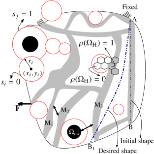
Figure 2: Design procedure for contact-aided shape morphing compliant mechanisms (CSMCMs). The design domain is discretized by hexagonal elements $\Omega_{\mathrm{H}}$. Negative circular masks $\Omega_{\mathrm{M}}$ (red circles) are used to remove material and also, to generate contact surfaces. Five parameters ($x_{i},\,y_{i},\,r_{i},\,s_{i},\,f_{i}$) define each mask. $s_{i}=1$ represents a contact surface (circular solids in black) within the $i^{\mathrm{th}}$ mask while $s_{i}=0$ implies no contact surface. $\rho(\Omega_{\mathrm{H}})=0$ implies a void element while $\rho(\Omega_{\mathrm{H}})=1$ indicates a filled element. Contact surfaces ($\Omega_{cs}$) interact (shown with double head arrows) with the mechanism (mutual contact), e.g., an interaction between member M₃ and $\Omega_{cs}$. In addition, the mechanism interacts with itself (self contact), e.g., contact between members M₁ and M₂. The desired final configuration of the link AB is shown. Fixed boundary(ies) of the domain, input force(s) and output path are also shown.

Hexagonal elements are used to parameterize the design domain. These elements provide edge connectivity between any two contiguous elements (Saxena and Saxena, 2007; Langelaar, 2007; Saxena, 2008; Talischi et al., 2009; Saxena, 2011; Kumar and Saxena, 2015; Singh et al., 2020) and thus, alleviate checkerboard patterns or alternating filled and void elements, and point connections naturally. Negative circular masks are employed to remove material and also, to generate contact surfaces within some of them (Kumar et al., 2016). In cases wherein only material removal (e.g. self contact) is to be performed, an $i^{\mathrm{th}}$ mask is defined via its center coordinates $(x_{i},\,y_{i})$ and radius $r_{i}$. Two more parameters $(s_{i},\,f_{i})$ are included within the definition of the mask, if an external (rigid) contact surface is also to be generated. Herein, $s_{i}$ and $f_{i}$ are binary and real fraction ($0<f_{i}<1$) variables, respectively. $s_{i}=1$ indicates generation of a contact surface with radius $f_{i}r_{i}$ within the mask, whereas $s_{i}=0$ means that no contact surface is generated. The material state of each element toggles between void, $\rho(\Omega_{\mathrm{H}})=0$, and solid, $\rho(\Omega_{\mathrm{H}})=1$, phases as positions and sizes of negative circular masks get updated. In each optimization iteration, all unexposed elements, i.e., elements with $\rho(\Omega_{\mathrm{H}})=1$ constitute the potential candidate design (Fig. 2). These designs contain many V-notches on their bounding surfaces (Fig. 3(a)). A boundary resolution and smoothing scheme (Kumar and Saxena, 2015), which shifts boundary nodes systematically is implemented, so that normals of the boundaries become well-defined (Fig. 3(b)). Mean value shape functions (Hormann and Floater, 2006) are employed for nonlinear finite element analysis. To evaluate contact forces and corresponding stiffness matrices, the augmented Lagrange multiplier method in conjunction with segment-to-segment contact approach is implemented Kumar (2017). The Newton-Raphson method is used to solve nonlinear mechanical equilibrium equations.

Prior to the analysis, a set of shape morphing nodes (SMNs) are selected in the design region. Elements containing those nodes are determined and termed shape morphing elements (SMEs). SMEs must always be a part of the potential intermediate candidate design, i.e., SMEs constitute a solid non-design region. The mutated negative masks which overlay on SMEs are shifted systematically such that all SMEs remain in their solid material state. The design vector is updated accordingly. An objective based on Fourier shape descriptors (Zahn and Roskies, 1972) is conceptualized to evaluate the error between the desired and actual shapes. The actual shape is defined by the updated nodal positions of SMNs after completion of the Newton-Raphson iterations. The objective is minimized by the stochastic hill-climber method (Kumar et al., 2015, 2017).

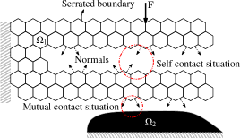
(a)

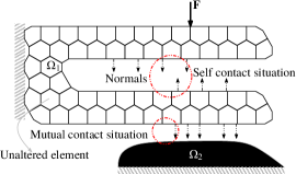
(b)

Figure 3: Two bodies $\Omega_{1}$ and $\Omega_{2}$ come into contact. (3(a)) $\Omega_{1}$ without boundary smoothing and (3(b)) $\Omega_{1}$ with boundary smoothing. Jumps in boundary normals are subdued with a boundary smoothing scheme. Self and mutual contact sites are depicted with dash-dotted red circles.

3 Problem formulation

When two bodies interact, they experience contact forces at their respective contact boundary facets (Fig. 4(b)). Typically, these forces depend on boundary normals (Wriggers, 2006). Jumps in normals are undesirable because they lead to non-convergence in contact analysis (Wriggers, 2006). Serrated boundary facets lead to discontinuity in boundary normals (Fig. 3(a)). To subdue serrations from the bounding surfaces, the boundary resolution and smoothing scheme (Kumar and Saxena, 2013, 2015) is incorporated.

3.1 Boundary resolution and smoothing

The boundary resolution and smoothing is accomplished in two steps. In the first, identification of boundary edges, which are not shared by two or more elements, is performed and hence, boundary nodes constituting such edges are recognized. In the second, boundary nodes are projected along their shortest perpendiculars on the straight segments joining the mid-points of the boundary edges. Such projections can be performed multiple times on the updated nodal coordinates (Kumar and Saxena, 2015).

Hexagonal elements are removed in two steps: (1) Elements which are overlaid by negative masks are removed and then, the smoothing is performed. (2) Elements which are not affected (Fig. 3(b)) by smoothing in the former step are also removed subsequently. This is equivalent to placing additional negative masks over such elements. The latter step helps achieve candidate CMs with slender members and thus, facilitate in their large deformation. Additionally, overall volume of the mechanism is reduced. At the end of the second step, all remaining hexagonal elements are considered in their regular shape, and boundary smoothing is performed again before contact finite element analysis is executed. As a consequence of the boundary smoothing, some boundary elements morph into concave elements (Kumar and Saxena, 2015). Mean value shape functions (Hormann and Floater, 2006) which can cater to generic polygonal shape finite elements are used for finite element analysis. For the sake of completeness, we briefly present the employed contact finite element formulation.

3.2 Contact finite element formulation

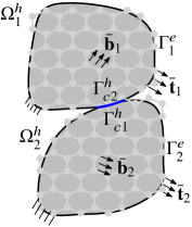
(a)

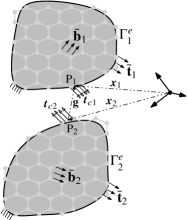
(b)

Figure 4: Two bodies $\Omega_{k}|_{k=1,2}$ (in discrete setting, $\Omega_{k}^{h}|_{k=1,2}$) with known surface tractions $\tilde{\mathbf{t}}_{k}$, volumetric body forces $\tilde{\mathbf{b}}_{k}$, and boundary conditions are depicted. When these bodies come into contact then contact surfaces $\Gamma_{ck}$ (or $\Gamma_{ck}^{h}$) and respective contact surface tractions $\bm{t}_{ck}$ appear. Consider points P${}_{1}\in\Gamma_{c1}$ and P${}_{2}\in\Gamma_{c2}$ with position vectors $\bm{x}_{1}$ and $\bm{x}_{2}$, respectively. Then the gap vector $\bm{g}$ is evaluated as $\bm{x}_{2}-\bm{x}_{1}$.

To evaluate contact forces and corresponding contact stiffness matrices, frictionless and adhesionless contact is assumed. Contact is modeled using the augmented Lagrange multiplier method in association with the Uzawa type (Bertsekas, 2014) algorithm while considering the segment-to-segment approach. Classical penalty method is employed in the inner loop whereas in the outer loop, the Lagrange multiplier is updated (Wriggers, 2006). In the classical penalty method, the contact traction $\bm{t}_{c}$ is defined as

$$\bm{t}_{c}=\begin{cases}-\epsilon_{n}g_{n}\bm{n}_{\text{p}}\qquad\,\,\,\,\text{for}\,\,g_{n}<0\\ \mathbf{0}~{}\qquad~{}\qquad\quad\text{for}\,\,g_{n}\geq 0\end{cases}$$ (1)

where $g_{n}=(\bm{x}-\bm{x}_{\text{p}})\cdot\bm{n}_{\text{p}}$ is the normal gap. $\bm{x}_{\text{p}}$ is the projection point of $\bm{x}\in\Gamma_{c1}^{h}$ on the surface $\Gamma_{c2}^{h}$. $\bm{n}_{p}$ is the unit normal at the projection point $\bm{x}_{\text{p}}$ which is determined by solving the following minimization problem

$$\bm{x}_{\text{p}}=\{\bm{x_{2}}:\min_{\bm{x}_{2}\in\Gamma_{c2}^{h}}||\bm{x}-\bm{x}_{2}||\,\,\forall\bm{x}\in\Gamma_{c1}^{h}\}.$$ (2)

In a finite element setting, the virtual work contribution of elemental contact forces can be written as

$$\mathbf{f}_{c}^{e}=-\int_{\Gamma_{c}^{e}}\mathbf{N}^{\mathrm{T}}\bm{t}_{c}^{e}\,\mathrm{d}a,$$ (3)

and by assembling all such $\mathbf{f}_{c}^{e}$, one can find the global contact force $\mathbf{f}_{\text{c}}$. $\mathbf{N}=[N_{1}\bm{I},\,N_{2}\bm{I}]$ with $N_{1}=\frac{1}{2}(1-\xi)$, $N_{2}=\frac{1}{2}(1+\xi)$ and $\xi\in[-1,\,1]$. Further, $\text{d}a$ is the elemental area and $\bm{I}$ is the identity tensor.

The discretized weak form of the mechanical equilibrium equations then leads to the global finite element equilibrium equations

$$\mathbf{f}(\mathbf{u})=\mathbf{f}_{\mathrm{int}}+\mathbf{f}_{\mathrm{c}}-\mathbf{f}_{\mathrm{ext}}=\mathbf{0},$$ (4)

where $\mathbf{f}_{\mathrm{int}},\,\mathbf{f}_{\mathrm{c}},\,\text{and}\,\mathbf{f}_{\mathrm{ext}}$ are the internal, contact and external forces, respectively. Eq. 4 is solved using the Newton-Raphson iterative method. One evaluates the elemental internal force $\mathbf{f}^{e}_{\mathrm{int}}$ as

$$\mathbf{f}^{e}_{\mathrm{int}}=\int_{\Omega_{k}^{h}}\mathbf{B}_{\mathrm{UL}}^{\mathrm{T}}\bm{\sigma}\,\mathrm{d}v,$$ (5)

where $\mathbf{B}_{\mathrm{UL}}$ is the discrete strain-displacement matrix (Bathe, 2006) of an element in the current configuration, and $\text{d}v$ is the elemental volume. For 2D cases such as plane strain, one can evaluate $\text{d}a=t\,\text{d}s$ and $\text{d}v=t\,\text{d}a$, where t is the thickness and $\text{d}s$ is the arc segment. $\bm{\sigma}$ is the Cauchy stress tensor evaluated using the nonlinear, isotropic, neo-Hookean material model (Zienkiewicz and Taylor, 2005)

$$\bm{\sigma} =\frac{\mu}{J}(\bm{F}\bm{F}^{\mathrm{T}}-\bm{I})+\frac{\lambda}{J}(\ln J)\bm{I},\qquad\ J=\text{det}\,\bm{F}$$ (6)

where $\mu={E}/{2/(1+\nu)}$ and $\lambda={2\mu\nu}/({1-2\nu})$ are Lame’s constants, and $\bm{F}=\text{Grad}\,\bm{u}+\bm{I}$ is the deformation gradient. Further, $E$ and $\nu$ are Young’s modulus and Possions’ ratio, respectively.

3.3 Formulation of objective function and optimization problem

An objective based on Fourier Shape Descriptors (FSDs) (Zahn and Roskies, 1972) is formulated and minimized. This objective lets a user to exercise individual control on the errors in shape, size and initial orientation between two curves (Ullah and Kota, 1997). First, a curve is closed in the clockwise sense such that it does not intersect itself. Then its Fourier coefficients are evaluated wherein the curve is parameterized using its normalized arc length.

Let $A_{n}^{k}$ and $B_{n}^{k}$ be the Fourier coefficients, $\theta^{k}$ and $L^{k}$ be the initial orientation and total length of the two curves, $k=a\,,\,d\,$ represent the actual and desired shapes, respectively. Further, $n$ is the total number of Fourier coefficients. One evaluates the FSDs objective as

$$f_{0}(\mathbf{v})=\lambda_{a}A_{\mathrm{{err}}}+\lambda_{b}B_{\mathrm{{err}}}+\lambda_{L}L_{\mathrm{{err}}}+\lambda_{\theta}\theta_{\mathrm{{err}}},$$ (7)

where $\lambda_{a},\,\lambda_{b},\,\lambda_{L},\,\text{and}\,\lambda_{\theta}$ are user defined weight parameters for the errors

$$A_{\mathrm{{err}}} =\sum_{i=1}^{n}(A_{i}^{d}-A_{i}^{a})^{2},\qquad B_{\mathrm{{err}}}=\sum_{i=1}^{n}(B_{i}^{d}-B_{i}^{a})^{2},\,$$ (8)

$$L_{\mathrm{{err}}} =(L^{d}-L^{a})^{2},\qquad\quad\theta_{\mathrm{{err}}}=(\theta^{d}-\theta^{a})^{2},$$

and $\mathbf{v}$ is the design vector. The units of the $\lambda$’s are chosen such that $f_{0}$ is dimensionless.The optimization problem then is

$$\underset{\mathbf{v}}{\text{min}} f(\mathbf{v})+\lambda_{v}(V-V^{*}),$$ (9)

$$\text{such that}, \mathbf{f}(\mathbf{u})=\mathbf{0};\,\,q_{L}\leq q_{i}\leq q_{U}|_{q_{i}=x_{i},\,y_{i},\,r_{i}}$$

$$s_{i}\,(=0\,\,\text{or}\,\,1)\,;\,\,f_{i}\,[\in(0,1)]$$

where $V^{*}$ and $V^{c}$ are the desired and current volumes of the CSMCM, and $\lambda_{v}$ is the volume penalization parameter. $\lambda_{v}=0$ is taken, when $V^{*}<V^{c}$, otherwise $\lambda_{v}=20$ is used. $q_{L}$ and $q_{U}$ denote the lower and upper limits for $q_{i}\in\mathbf{v}$.

3.4 Hill climber search

Let the total number of overlaid negative circular masks be N_m. Each mask is defined via its $x,\,y,\,r,\,s,\,\text{and}\,f$ variables. The design vector $\mathbf{v}$ consists of $5$N_m variables. One sets a probability parameter $pr\,(=0.08)$ for each variable $d\in\mathbf{v}$. In each optimization iteration, one generates a random number $\chi$. If $\chi<pr$, the corresponding variable is altered as $d_{\mathrm{new}}=d_{\mathrm{old}}\pm(\kappa\times m)$, where $0<\kappa<1$ is a random number and $m$ is set to $10\%$ of the domain size, $\max(L_{1},\,L_{2})$. This mutation leads to a new design vector $\mathbf{v}_{\mathrm{new}}$. $s_{i}$ which indicates a contact surface generation is mutated as, if $\chi<pr$ and $\kappa<0.50$, $s_{i}=1$, else $s_{i}=0$. Likewise, $f_{i}\in[0,\,1]$ is also mutated. The magnitude of input force $F$ is also taken as a design variable (Mankame and Ananthasuresh, 2007) and updated as $F_{\text{new}}=F_{\text{old}}\pm(\kappa\times m)$. At this instance, if the input location, output location (member) and some fixed (boundary) conditions are available in the new design, then one evaluates the FSDs objective $f_{\mathrm{new}}$ as per design vector $\mathbf{v}_{\mathrm{new}}$, otherwise the design is penalized. If $f_{\mathrm{new}}<f_{\mathrm{old}}$, the design vector is updated. The process is continued until the maximum number of iterations is reached or terminated when it is found that the change in objective value for 10 successive optimization iteration is less than $\Delta f=0.01$.

Parameter’s name	Units	Value
Design domain	—	30$\Omega_{\mathrm{H}}\times$30$\Omega_{\mathrm{H}}$
Maximum radius of $\Omega_{\mathrm{M}}$	mm	8.0
Minimum radius of $\Omega_{\mathrm{M}}$	mm	0.1
Maximum # of iterations	—	5000
Young’s modulus ($E$)	MPa	2100
Poisson’s ratio	—	0.33
Permitted volume fraction ($\frac{V^{*}}{V}$)	—	0.30
Mutation probability	—	0.08
Contact surface radii factor	—	0.75
Maximum mutation size ($m_{\mathrm{{max}}}$)	—	5
Upper limit of the load ($\bm{F}_{\mathrm{Upp}}$)	N	1000
Lower limit of the load ($\bm{F}_{\mathrm{Low}}$)	N	-1000
Weight of $a_{\mathrm{err}}$ ($\lambda_{\mathrm{a}}$)	${\mathrm{rad}}^{-2}$	100
Weight of $b_{\mathrm{err}}$ ($\lambda_{\mathrm{b}}$)	${\mathrm{rad}}^{-2}$	100
Weight of length error ($\lambda_{\mathrm{L}}$)	${\mathrm{mm}}^{-1}$	1
Weight of orientation error ($\lambda_{\mathrm{\theta}}$)	${\mathrm{rad}}^{-2}$	1
Boundary smoothing steps ($\beta$)	—	10
Penalty parameter ($\epsilon_{n}$)	N/mm3	$60E/L_{2}$
Penalty parameter ($\epsilon_{s}$)	N/mm3	$5E/L_{2}$

Table 1: Parameters used in the synthesis for Example 1, Example 2 and Example 3. $\epsilon_{n}$ and $\epsilon_{s}$ are the penalty parameters for mutual and self contact, respectively.

4 Numerical examples and discussion

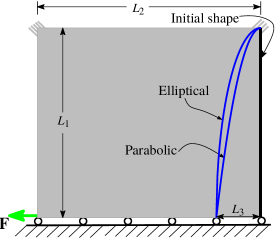
(a)

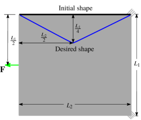
(b)

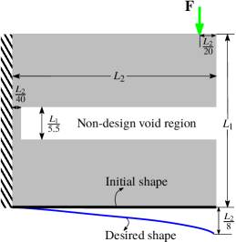
(c)

Figure 5: (5(a)) Design specification for Example 1 and Example 2, (5(b)) Design specification for Example 3 and (5(c)) Design specification for Example 4. For Example 1, Example 2 and Example 3, $L_{1}=30\frac{3}{2}$\mathrm{mm}$,\,L_{2}=30\sqrt{3}$\mathrm{mm}$,\,L_{3}=\frac{L_{2}}{3\sqrt{3}}$\mathrm{mm}$$. For Example 4, $L_{1}=39\frac{3}{2}$\mathrm{mm}$,\,L_{2}=40\sqrt{3}$\mathrm{mm}$$.

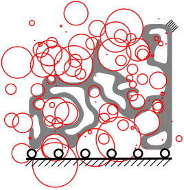
(a)

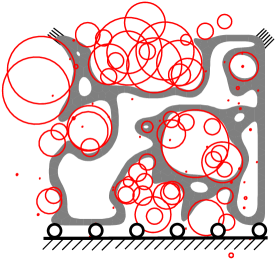
(b)

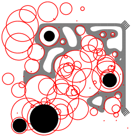
(c)

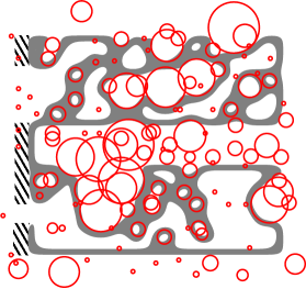
(d)

Figure 6: Solutions to Example 1, Example 2, Example 3 and Example 4 with boundary conditions are shown in figures (a), (b), (c) and (d), respectively. The final positions and sizes of circular masks (red) are also depicted.

Efficacy of the presented method is demonstrated via four contact-aided shape morphing compliant mechanisms which are synthesized for different prescribed shapes (i.e. parabolic, elliptical, and V-shape) shown in Fig. 5. The design specification is also depicted and various parameters are tabulated in Table 1. Plane-strain condition is assumed. The total number of Fourier coefficients is fixed to 50. The active set strategy in conjunction with contact-pairs detection scheme presented in Kumar et al. (2019b) is used to determine activeness and inactiveness of self and mutual contact modes.

4.1 Example 1

The symmetric half design domain specifications and the desired parabolic profile for this example are depicted in Fig. 5(a). The left and right corners of the top edge of the symmetric half design domain are fixed (Fig. 5(a)). To achieve the optimized compliant mechanism, $12$ masks in horizontal and $8$ masks in the vertical directions are employed. Only self contact is permitted and hence, masks are not required to generate rigid contact surfaces.

The final solution is obtained after $715$ optimization iterations. The final symmetric half result is suitably converted into a full mechanism (Fig. 6(a)). Various configurations at different deformed states are shown in Fig. 7. The figure also shows two locations of self contact encircled in dash-dotted red circles. The obtained optimum actuation force is $-100.59$ N in the horizontal direction. Self contact occurs much later in the deformation history and does not influence the actual shape much. One can notice that the final mechanism has some extra appendages that mechanically may not be contributing significantly and thus, those may be removed in the post processing step.

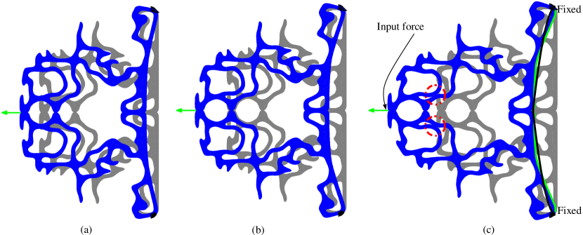
Figure 7: Example 1: Three deformed configurations (blue) are overlayed on the undeformed mechanism (gray). Figure (c) depicts the desired (black curve) and actual (green curve) shapes of the specified vertical member. Active contact locations are depicted using dash-dotted red circles. The input force and boundary conditions are also shown.

4.2 Example 2

The design specifications, optimization parameters, and the number of masks used are the same as those for Example 1, however, the final desired shape sought is elliptical (Fig. 5(a)).

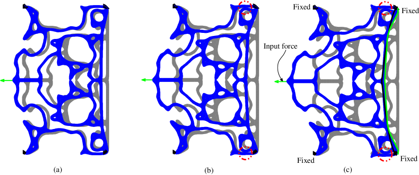
Figure 8: Example 2: Three deformed configurations (blue) are depicted with the undeformed mechanism (gray). The desired (black curve) and actual (green curve) shapes of the specified vertical member are shown in (c). Dash-dotted red circles are used to depict active contact locations. The input force and boundary conditions are also shown.

The optimized design is shown in Fig. 6(b). The final positions and shapes of the negative masks are also depicted. Deformed configurations of the full mechanism at different states are shown in Fig. 8. While deforming, the mechanism experiences self contact at two locations (Fig. 8). The final mechanism is obtained after $782$ optimization iterations with $-96.64$ N actuating force in the horizontal direction. Self contact happens much earlier in the deformation history, which helps achieve the actual elliptical profile, very close to the desired shape (Table 2).

4.3 Example 3

The design specifications for the third example are shown in Fig. 5(b). The same design parameters are used as for Example 1. The top and bottom corners of the right edge of the design domain are fixed. We take 10 masks in each direction for optimization. The masks are permitted to generate contact surfaces, i.e., 5 design parameters are used for each mask. This example is solved to achieve a V-shape for the specified edge (Fig. 5(b)). Note that in a continuum setting, getting such desired shapes is only possible if one uses very fine mesh and/or if there is discontinuity/notch at that boundary. For coarse meshes this is an extreme test case for the proposed mechanism design methodology.

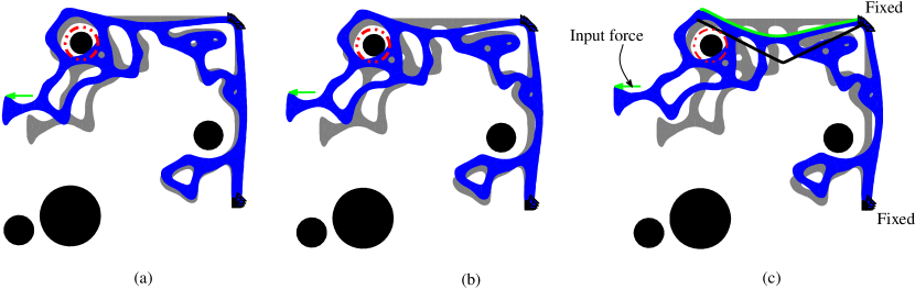
Figure 9: Example 3: Three deformed configurations (blue) along with input force and boundary conditions are overlayed on the undeformed mechanism (gray). Figure (c) depicts the desired (black curve) and actual (green curve) shapes of the specified horizontal member. The active contact surface is depicted with dash-dotted red circles.

The optimum solution (Fig. 6(c)) is obtained after $947$ optimization iterations. The mechanism interacts with only one contact surface though many such surfaces are present (Fig. 9). The final input force in the horizontal direction is $-96.30$ N. Various deformed configurations with active contact locations, actuation force, boundary condition are depicted in Fig. 9. Herein, mutual contact occurs much earlier in the deformation history. It is reckoned that the relative frictionless slip between the rigid surface and the loop (top left) contributes significantly to achieving a shape close to the ‘V’ profile. However, the desired ‘kink’ is not observed, this is because continuum surface deformations are usually smooth despite the presence of contact.

4.4 Example 4

The design domain specifications for Example 4 are displayed in Fig. 5(c). The left edge of the domain is fixed. A non-design void region of size $\frac{39L_{2}}{40}\times\frac{L_{1}}{5.5}$, symmetric to the center of the domain, as illustrated in the figure, is considered. An input force is applied on the top edge as depicted in Fig. 5(c). The initial and desired shapes of a potential contact-aided compliant mechanism are indicated in Fig. 5(c). $40\times 39$ hexagonal elements are used to discretize the design domain. We employ 12 and 10 negative masks along the $x-$ and $y-$directions, respectively. Other design parameters are the same as those mentioned in Table 1. Masks are permitted to remove only material but not to generate contact surfaces, thus contact can only occur as self contact between flexible members.

Figure 10: Three deformed configurations (blue) are overlayed on the undeformed mechanism (gray). Figure (c) depicts the desired (black curve) and actual (green curve) shapes of the specified horizontal member. Active contact locations are depicted using dash-dotted red circles. The input force and boundary conditions are also shown. The desired shape cannot be obtained unless there is contact between the top and bottom subregions.

The final solution of the mechanism with final shape and size of the masks with their position is shown in Fig. 6(d). Different configurations at different instances are illustrated in Fig. 10. Self contact sites are also depicted in the figure using the dash-dotted red circles. The final input force is $-$$25.0\text{\,}\mathrm{N}$ in the $y-$direction. One can notice that the mechanism achieves the desired profile while deforming due to self contact. Thus, self contact can play a vital role in achieving the final desired profile of a SMCM.

4.5 Comparison between the desired and actual curves

The error in shape and size between the two curves is formulated with respect to respective Fourier coefficients in terms of $R_{m}=\sqrt{A_{m}^{2}+B_{m}^{2}}$, where $R_{m}|_{(m=1,2,\cdots,n)}$ are curve invariants (Zahn and Roskies, 1972). The overall relative change in shape $\zeta_{s}$ is evaluated as

$$\zeta_{s}=\bigg{[}\frac{1}{n}\sum_{m=1}^{n}\frac{|R_{m}^{d}-R_{m}^{a}|}{R_{n}^{d}}\bigg{]},$$ (10)

where $R_{m}^{d}$ and $R_{m}^{a}$ are invariants corresponding to the desired and actual curves respectively. Likewise, the relative change in lengths is evaluated as $\zeta_{l}=\frac{|L^{d}-L^{a}|}{L^{d}}$.

Table 2: Percentage change in FSD coefficients and length of actual curve of CSMCMs with respect to their corresponding desired curves

Mechanisms	$\zeta_{s}$ (%)	$\zeta_{l}$ (%)
Example 1	0.394	4.645
Example 2	0.233	5.962
Example 3	0.557	12.722
Example 4	1.99	3.12

Table 2 depicts the comparison of $\zeta_{s}$ and $\zeta_{l}$ for the presented examples. One notices for each problem $\zeta_{s}$ is within 2% (Table 2), indicating good shape agreement between the actual and desired curves. We notice 12.72% length error between the desired and actual curves for Example 3.

4.6 Verification of the deformed profiles

ABAQUS is used to appraise the accuracy of the presented design approach by comparing the deformed profiles for the optimized designs with those obtained by ABAQUS analyses.

Table 3: Percentage change in FSDs coefficients and length of actual curve of CSMCMs with respect to their corresponding curves obtained using ABAQUS

Mechanisms	$\zeta_{s}$ (%)	$\zeta_{l}$ (%)
Example 1	0.1808	7.043
Example 2	0.1126	5.817
Example 3	0.047	0.67
Example 4	1.97	3.01

(a)

(b)

(c)

(d)

Figure 11: The deformed profiles of the actual curves for Example 1, Example 2, Example 3 and Example 4 and those obtained using ABAQUS are depicted in (11(a)), (11(b)), (11(c)), and (11(d)), respectively. Horizontal and vertical axes of the plots represent $x-$ and $y-$positions of the curves, respectively.

To perform the ABAQUS nonlinear contact analyses, (i) the optimal forces, (ii) boundary conditions, and (iii) active contact locations (self and/or mutual) of the optimized solutions (Fig. 6) in association with the neo-Hookean material model, are used. Using the information of boundary nodes, the optimized results are converted into respective CAD models. Four-noded plain-strain elements (CPE4I) are employed to describe the extracted CAD model of the mechanism. The actual profiles and those obtained using ABAQUS for the respective examples, are depicted in Fig. 11. The analyses indicate that the obtained deformed shapes closely follow the respective actual deformed shapes for the presented examples (Fig. 11 and Table 3).

4.7 Influence of friction

In this section, we present a study of frictional contact surfaces on the performance (the ability to obtain the desired deformed profiles) of the final mechanisms in ABAQUS by considering different friction coefficients. The presented topology optimization approach though does not account for frictional contact, it can be readily added using the formulation mentioned in (Sauer and De Lorenzis, 2015).

Table 4: Percentage change in FSD coefficients and length of curve obtained with friction to those without friction using ABAQUS

Mechanisms	$\mu_{f}=0.25$		$\mu_{f}=0.35$
	$\zeta_{s}$ (%)	$\zeta_{l}$ (%)	$\zeta_{s}$ (%)	$\zeta_{l}$ (%)
Example 1	0.00023	0.0015	0.00030	0.0018
Example 2	0.0003	0.0016	0.00035	0.0017
Example 3	0.0173	2.038	0.0207	2.1314
Example 4	0.0054	0.083	0.0077	0.12

(a)

(b)

(c)

(d)

Figure 12: The obtained deformed profiles of the actual curves with different frictional coefficients $\mu_{f}$ using ABAQUS are overlaid and depicted for Example 1, Example 2, Example 3 and Example 4 in (12(a)), (12(b)), (12(c)), and (12(d)), respectively. Horizontal and vertical axes of the plots represent $x-$ and $y-$positions of the curves, respectively.

The deformed shapes of the pre-sepcified constituting members of the respective examples with $\mu_{f}=0$, $\mu_{f}=0.25$ and $\mu_{f}=0.35$ are overlaid and compared in Fig. 12. Percentage change in the FSDs coefficients and lengths of the deformed profiles with respect to $\mu_{f}=0$, are given in Table 4. One notices that friction does not alter the quantitative and/or qualitative behavior of the deformed shapes (Fig. 12 and Table 4). However, this may not be the case in a situation where contact surfaces are comparatively bigger in shape.

4.8 Presence of small holes

One notices a few small holes in the final designs of Example 2, Example 3 and Example 4 (Fig. 6). These holes appear due to the localized removal of either one/two FEs by (a group of) circular masks or one/two unaffected FEs (Fig. 3(b)). The respective modified designs are obtained after removing those small holes. The nonlinear contact FE analyses in ABAQUS are performed using the final and their respective modified designs. The obtained end-compliance values are reported in Table 5. The differences in values of the end-compliance for all these examples are found to be below 1%, thus those small holes can be removed in a post processing step.

Table 5: End-compliance values

Mechanism	Original design	Modified design	Difference (%)
	End-compliance (Nmm)
Example 2	1107.50	1194.47	0.79
Example 3	1093.97	1088.20	0.053
Example 4	497.87	495.66	0.045

5 Closure

An approach to synthesize contact-aided shape morphing compliant mechanisms using hexagonal elements and negative circular masks, is presented. Self and/or mutual contact modes are permitted. Geometric and material nonlinearities are considered wherein a neo-Hookean material model is employed. Versatility of the presented method is demonstrated via four examples with various desired shapes. The optimized mechanisms for Example 1, Example 2 and Example 4 experience self contact while achieving their desired shapes, whereas mutual contact helps achieve the actual shape similar to the its desired one for Example 3. By and large, there is a good agreement between the desired and actual curves as differences in shape and size measure for these curves are within $1\%$.

The augmented Lagrange multiplier method is used considering a segment-to-segment contact model. The implemented boundary smoothing reduces jumps in the normals of the boundary facets thereof and facilitates convergence of the contact analysis. The nonlinear mechanical equilibrium equations are solved using the Newton-Raphson method. An FSDs based objective is formulated and minimized, which permits to have individual control over the characteristics of a curve. Hill-climber, a zero-order search algorithm, is used.

The optimized mechanisms are analyzed in ABAQUS using the respective actuating force, boundary conditions, and active contact locations. It is noticed that the deformed profiles obtained by the approach and those by ABAQUS are very close to each-other. Analyses considering frictional contact surfaces are also performed in ABAQUS. It is noted that friction does not alter the behavior of the deformed curves much. In future, we aim to design special characteristic mechanisms, e.g., with negative stiffness or zero-stiffness and statically balanced mechanisms in association with contact constraints, which can find applications in medical devices.

References

- Ananthasuresh et al. (1994) Ananthasuresh GK, Kota S, Kikuchi N (1994) Strategies for systematic synthesis of compliant mems. In: Proceedings of the 1994 ASME winter annual meeting, pp 677–686
- Bathe (2006) Bathe KJ (2006) Finite element procedures. Englewood Cliffs, NJ: Prentice-Hall.
- Bertsekas (2014) Bertsekas DP (2014) Constrained optimization and Lagrange multiplier methods. Academic press
- Cannon and Howell (2005) Cannon JR, Howell LL (2005) A compliant contact-aided revolute joint. Mechanism and Machine Theory 40(11):1273–1293
- Frecker et al. (1997) Frecker M, Ananthasuresh GK, Nishiwaki S, Kikuchi N, Kota S (1997) Topological synthesis of compliant mechanisms using multi-criteria optimization. Journal of Mechanical design 119(2):238–245
- Frecker et al. (1999) Frecker M, Kikuchi N, Kota S (1999) Topology optimization of compliant mechanisms with multiple outputs. Structural Optimization 17(4):269–278
- Hormann and Floater (2006) Hormann K, Floater MS (2006) Mean value coordinates for arbitrary planar polygons. ACM Transactions on Graphics (TOG) 25(4):1424–1441
- Howell (2001) Howell LL (2001) Compliant mechanisms. John Wiley & Sons
- Kumar (2017) Kumar P (2017) Synthesis of large deformable contact-aided compliant mechanisms using hexagonal cells and negative circular masks. PhD thesis, Indian Institute of Technology Kanpur
- Kumar and Saxena (2013) Kumar P, Saxena A (2013) On embedded recursive boundary smoothing in topology optimization with polygonal mesh and negative masks. AMM india, IIT Roorkee pp 568–575
- Kumar and Saxena (2015) Kumar P, Saxena A (2015) On topology optimization with embedded boundary resolution and smoothing. Structural and Multidisciplinary Optimization 52(6):1135–1159
- Kumar et al. (2015) Kumar P, Sauer RA, Saxena A (2015) On synthesis of contact aided compliant mechanisms using the material mask overlay method. In: ASME 2015 International Design Engineering Technical Conferences and Computers and Information in Engineering Conference, American Society of Mechanical Engineers, pp V05AT08A017–V05AT08A017
- Kumar et al. (2016) Kumar P, Sauer RA, Saxena A (2016) Synthesis of path-generating contact-aided compliant mechanisms using the material mask overlay method. Journal of Mechanical Design 138(6):062301
- Kumar et al. (2017) Kumar P, Saxena A, Sauer RA (2017) Implementation of self contact in path generating compliant mechanisms. In: Microactuators and Micromechanisms, Springer, pp 251–261
- Kumar et al. (2019a) Kumar P, Fanzio P, Sasso L, Langelaar M (2019a) Compliant fluidic control structures: Concept and synthesis approach. Computers & Structures 216:26–39
- Kumar et al. (2019b) Kumar P, Saxena A, Sauer RA (2019b) Computational synthesis of large deformation compliant mechanisms undergoing self and mutual contact. Journal of Mechanical Design 141(1):012302
- Kumar et al. (2020) Kumar P, Schmidleithner C, Larsen NB, Sigmund O (2020) Topology optimization and 3D-printing of large deformation compliant mechanisms for straining biological tissues. Structural and Multidisciplinary Optimization p (In Press)
- Langelaar (2007) Langelaar M (2007) The use of convex uniform honeycomb tessellations in structural topology optimization. In: 7th world congress on structural and multidisciplinary optimization, Seoul, South Korea, May, pp 21–25
- Larsen et al. (1997) Larsen UD, Signund O, Bouwsta S (1997) Design and fabrication of compliant micromechanisms and structures with negative poisson’s ratio. Journal of Microelectromechanical Systems 6(2):99–106
- Lu and Kota (2003) Lu KJ, Kota S (2003) Design of compliant mechanisms for morphing structural shapes. Journal of intelligent material systems and structures 14(6):379–391
- Mankame and Ananthasuresh (2007) Mankame N, Ananthasuresh GK (2007) Synthesis of contact-aided compliant mechanisms for non-smooth path generation. International Journal for Numerical Methods in Engineering 69(12):2564–2605
- Mankame and Ananthasuresh (2004) Mankame ND, Ananthasuresh GK (2004) Topology optimization for synthesis of contact-aided compliant mechanisms using regularized contact modeling. Computers & structures 82(15):1267–1290
- Mehta et al. (2008) Mehta V, Frecker M, Lesieutre G (2008) Contact-aided compliant mechanisms for morphing aircraft skin. In: Modeling, Signal Processing, and Control for Smart Structures 2008, International Society for Optics and Photonics, vol 6926, p 69260C
- Mehta et al. (2009) Mehta V, Frecker M, Lesieutre GA (2009) Stress relief in contact-aided compliant cellular mechanisms. Journal of Mechanical Design 131(9):091009
- Midha and Howell (1994) Midha A, Howell L (1994) A method for the design of compliant mechanisms with small-length flexural pivots. ASME J Mech Des 116:280–290
- Pedersen et al. (2001) Pedersen CB, Buhl T, Sigmund O (2001) Topology synthesis of large-displacement compliant mechanisms. International Journal for numerical methods in engineering 50(12):2683–2705
- Rai et al. (2007) Rai AK, Saxena A, Mankame ND (2007) Synthesis of path generating compliant mechanisms using initially curved frame elements. Journal of Mechanical Design 129(10):1056–1063
- Ramrakhyani et al. (2005) Ramrakhyani DS, Lesieutre GA, Frecker MI, Bharti S (2005) Aircraft structural morphing using tendon-actuated compliant cellular trusses. Journal of aircraft 42(6):1614–1620
- Reddy et al. (2012) Reddy BVSN, Naik SV, Saxena A (2012) Systematic synthesis of large displacement contact-aided monolithic compliant mechanisms. Journal of Mechanical Design 134(1):011007
- Saggere and Kota (1999) Saggere L, Kota S (1999) Static shape control of smart structures using compliant mechanisms. AIAA journal 37(5):572–578
- Sauer and De Lorenzis (2015) Sauer RA, De Lorenzis L (2015) An unbiased computational contact formulation for 3d friction. International Journal for Numerical Methods in Engineering 101(4):251–280
- Saxena (2005) Saxena A (2005) Topology design of large displacement compliant mechanisms with multiple materials and multiple output ports. Structural and Multidisciplinary Optimization 30(6):477–490
- Saxena (2008) Saxena A (2008) A material-mask overlay strategy for continuum topology optimization of compliant mechanisms using honeycomb discretization. Journal of Mechanical Design 130:082304
- Saxena (2011) Saxena A (2011) Topology design with negative masks using gradient search. Structural and Multidisciplinary Optimization 44(5):629–649
- Saxena and Ananthasuresh (2000) Saxena A, Ananthasuresh GK (2000) On an optimal property of compliant topologies. Structural and multidisciplinary optimization 19(1):36–49
- Saxena and Ananthasuresh (2001) Saxena A, Ananthasuresh GK (2001) Topology synthesis of compliant mechanisms for nonlinear force-deflection and curved path specifications. Journal of Mechanical Design 123(1):33–42
- Saxena and Saxena (2007) Saxena R, Saxena A (2007) On honeycomb representation and sigmoid material assignment in optimal topology synthesis of compliant mechanisms. Finite Elements in Analysis and Design 43(14):1082–1098
- Sigmund (1997) Sigmund O (1997) On the design of compliant mechanisms using topology optimization. Journal of Structural Mechanics 25(4):493–524
- Singh et al. (2020) Singh N, Kumar P, Saxena A (2020) On topology optimization with elliptical masks and honeycomb tessellation with explicit length scale constraints. Structural and Multidisciplinary Optimization pp 1–25
- Talischi et al. (2009) Talischi C, Paulino GH, Le CH (2009) Honeycomb wachspress finite elements for structural topology optimization. Structural and Multidisciplinary Optimization 37(6):569–583
- Tummala et al. (2013) Tummala Y, Frecker MI, Wissa A, Hubbard Jr JE (2013) Design and optimization of a bend-and-sweep compliant mechanism. Smart materials and structures 22(9):094019
- Tummala et al. (2014) Tummala Y, Wissa A, Frecker M, Hubbard JE (2014) Design and optimization of a contact-aided compliant mechanism for passive bending. Journal of Mechanisms and Robotics 6(3):031013
- Ullah and Kota (1997) Ullah I, Kota S (1997) Optimal synthesis of mechanisms for path generation using fourier descriptors and global search methods. Journal of Mechanical Design 119(4):504–510
- Wissa et al. (2012) Wissa A, Tummala Y, Hubbard Jr J, Frecker M (2012) Passively morphing ornithopter wings constructed using a novel compliant spine: design and testing. Smart Materials and Structures 21(9):094028
- Wriggers (2006) Wriggers P (2006) Computational contact mechanics, vol 30167. Springer
- Zahn and Roskies (1972) Zahn CT, Roskies RZ (1972) Fourier descriptors for plane closed curves. Computers, IEEE Transactions on 100(3):269–281
- Zhu et al. (2020) Zhu B, Zhang X, Zhang H, Liang J, Zang H, Li H, Wang R (2020) Design of compliant mechanisms using continuum topology optimization: A review. Mechanism and Machine Theory 143:103622
- Zienkiewicz and Taylor (2005) Zienkiewicz OC, Taylor RL (2005) The finite element method for solid and structural mechanics. Butterworth-heinemann