Minimax Estimation of Conditional Moment Models

Abstract

We develop an approach for estimating models described via conditional moment restrictions, with a prototypical application being non-parametric instrumental variable regression. We introduce a min-max criterion function, under which the estimation problem can be thought of as solving a zero-sum game between a modeler who is optimizing over the hypothesis space of the target model and an adversary who identifies violating moments over a test function space. We analyze the statistical estimation rate of the resulting estimator for arbitrary hypothesis spaces, with respect to an appropriate analogue of the mean squared error metric, for ill-posed inverse problems. We show that when the minimax criterion is regularized with a second moment penalty on the test function and the test function space is sufficiently rich, then the estimation rate scales with the critical radius of the hypothesis and test function spaces, a quantity which typically gives tight fast rates. Our main result follows from a novel localized Rademacher analysis of statistical learning problems defined via minimax objectives. We provide applications of our main results for several hypothesis spaces used in practice such as: reproducing kernel Hilbert spaces, high dimensional sparse linear functions, spaces defined via shape constraints, ensemble estimators such as random forests, and neural networks. For each of these applications we provide computationally efficient optimization methods for solving the corresponding minimax problem (e.g. stochastic first-order heuristics for neural networks). In several applications, we show how our modified mean squared error rate, combined with conditions that bound the ill-posedness of the inverse problem, lead to mean squared error rates. We conclude with an extensive experimental analysis of the proposed methods.

.tocmtchapter mtchaptersubsection mtappendixnone

1 Introduction

Understanding how policy choices affect social systems requires an understanding of the underlying causal relationships between them. To measure these causal relationships, social scientists look to either field experiments, or quasi-experimental variation in observational data. Most observational studies rely on assumptions that can be formalized in moment conditions. This is the basis of the estimation approach known as generalized method of moments (GMM) (Hansen, 1982).

While GMM is an incredibly flexible estimation approach, it suffers from some drawbacks. The underlying independence (randomization) assumptions often imply an infinite number of moment conditions. Imposing all of them is infeasible with finite data, but it is hard to know which ones to select. For some special cases, asymptotic theory provides some guidance, but it is not clear that this guidance translates well when the data is finite and/or the models are non-parametric. Given the increasing availability of data and new machine learning approaches, researchers and data scientists may want to apply adaptive non-parametric learners such as reproducing kernel Hilbert spaces, high-dimensional regularized linear models, neural networks and random forests to these GMM estimation problems, but this requires a way of finding solutions to the moment conditions within complex hypothesis classes imposed by the learner and selecting moment conditions that are adapted to the hypothesis class of the learner.

Most recent theoretical developments in machine learning and high-dimensional statistics are founded on statistical learning theory: formulate a loss function (typically strongly convex with respect to the output of the hypothesis), whose minimizer over the hypothesis space is the desired solution; typically referred to as an $M$-estimator. Being able to frame the problem as an $M$-estimation problem with a strongly convex function, leads to many desirable properties : i) tight generalization bounds and mean squared error rates based on localized notions of statistical complexity can be invoked to provide tight and fast finite sample rates with minimal assumptions (Bartlett et al., 2005; Wainwright, 2019), ii) regularization can be invoked to make the estimation adaptive to the complexity of the true hypothesis space, without knowledge of that complexity (Lecué and Mendelson, 2018, 2017; Negahban et al., 2012), iii) the computational problem can be typically efficiently solved via first order methods that can scale massively (Agarwal et al., 2014; Rahimi and Recht, 2008; Le, 2013; Sra et al., 2012; Bottou et al., 2007). This formulation is seemingly at odds with the method of moments language, as many times the moment conditions do not correspond to the gradient of some loss function and this problem is exacerbated in the case of non-parametric endogenous regression problems (i.e. when the instruments in the observational study does not coincide with the treatments). The problem is: Can we develop an analogue of modern statistical learning theory of $M$-estimators, for non-parametric problems defined via moment restrictions?

Our starting point is a set of conditional moment restrictions:

$$\mathbb{E}[y-h(x)\mid z]=0$$ (1)

where $y$ is an outcome of interest, $x$ is a vector of treatments and $z$ is a vector of instruments.

To obtain a criterion function, we first move to an unconditional moment formulation, where the moment restrictions are products of the moment conditions and test functions in the instruments. We then take as our criterion function the maximum moment deviation over the set of test functions, where the set of test functions is potentially infinite.

$$h_{0}=\operatorname*{arg\,inf}_{h\in{\mathcal{H}}}\sup_{f\in{\mathcal{F}}}\mathbb{E}[(y-h(x))f(z)]=:\Psi(h,f)$$ (2)

We show that as long as the set of test functions ${\mathcal{F}}$ contains all functions of the form $f(z)=\mathbb{E}[h(x)-h^{\prime}(x)\mid z]$ for $h,h^{\prime}\in{\mathcal{H}}$, then such an estimator achieves a projected MSE rate that scales with the critical radius of the function classes ${\mathcal{F}}$, ${\mathcal{H}}$ and their tensor product class (i.e. functions of the form $f(z)\cdot h(x)$, with $f\in{\mathcal{F}}$ and $h\in{\mathcal{H}}$). The critical radius captures information theoretically optimal rates for many function classes of interest and thereby this main theorem can be used to derive tight estimation rates for many hypothesis spaces. Moreover, if the regularization terms relate to the squared norms of $h,f$ in their corresponding spaces, then the estimation error scales with the norm of the true hypothesis, without knowledge of this norm.

We offer several applications of our main theorems for several hypothesis spaces of practical interest, such as reproducing kernel Hilbert spaces (RKHS), sparse linear functions, functions defined via shape restrictions, neural networks and random forests. For many of these estimators, we offer optimization algorithms with performance guarantees. As we illustrate in extensive simulation studies, different estimators are best in different regimes.

Related work

The non-parametric IV problem has a long history in econometrics Newey and Powell (2003); Blundell et al. (2007); Chen and Pouzo (2012); Chen and Christensen (2018); Hall et al. (2005); Horowitz (2007, 2011); Darolles et al. (2011); Chen and Pouzo (2009). Arguably the closest to our work is that of Chen and Pouzo (2012), who consider estimation of non-parametric function classes and estimation via the method of sieves and a penalized minimum distance estimator of the form: $\min_{h\in{\mathcal{H}}}\mathbb{E}[\mathbb{E}[y-h(x)\mid z]^{2}]+\lambda R(h)$, where $R(h)$ is a regularizer. As we show in Appendix A, our estimator can be interpreted asymptotically as a minimum distance estimator, albeit our estimation method applies to arbitrary function classes and non just linear sieves. There is also a growing body of work in the machine learning literature on the non-parametric instrumental variable regression problem Hartford et al. (2017); Bennett et al. (2019); Singh et al. (2019); Muandet et al. (2019, 2020). Our work has several features that draw connections to each of these works, e.g. Bennett et al. (2019); Muandet et al. (2019, 2020) also use a minimax criterion and Bennett et al. (2019); Muandet et al. (2019) also impose some form of variance penalty on the test function. We discuss subtle differences in Appendix A. Moreover, Singh et al. (2019); Muandet et al. (2019) also study RKHS hypothesis spaces and Hartford et al. (2017); Bennett et al. (2019) also study neural net hypothesis spaces. None of these prior works provide finite sample estimation error rates for arbitrary hypothesis spaces and typically only show consistency for the particular hypothesis space analyzed (with the exception of Singh et al. (2019), who provide finite sample rates for RKHS spaces, under further conditions on the smoothness of the true hypothesis). In Appendix A we offer a more detailed exposition on the related work and how it relates to our main results.

2 Preliminary Definitions

We consider the problem of estimating a flexible econometric model that satisfies a set of conditional moment restrictions presented in 1 (see also Appendix B), where $z\in{\mathcal{Z}}\subseteq\mathbb{R}^{d}$, $X\in{\mathcal{X}}\subseteq\mathbb{R}^{p}$, $y\in\mathbb{R}$, $h\in{\mathcal{H}}\subseteq({\mathcal{X}}\to\mathbb{R})$ for ${\mathcal{H}}$ a hypothesis space. For simplicity of notation we will also denote with $\psi(y;h(x))=y-h(x)$. The truth is some model $h_{0}$ that satisfies all the moment restrictions.

We assume we have access to a set of $n$ i.i.d. sample points $\{v_{i}:=(y_{i},x_{i},z_{i})\}_{i=1}^{n}$ drawn from some unknown distribution $\mathcal{D}$ that satisfies the moment condition in Equation 1. We will analyze estimators that optimize an empirical analogue of the minimax objective presented in the introduction, potentially adding norm-based penalties $\Phi:{\mathcal{F}}\to\mathbb{R}_{+}$, $R:{\mathcal{H}}\to\mathbb{R}_{+}$:

$$\hat{h}:=\operatorname*{arg\,min}_{h\in{\mathcal{H}}}\sup_{f\in{\mathcal{F}}}\Psi_{n}(h,f)-\lambda\,\Phi(f)+\mu\,R(h)$$ (3)

where $\Psi_{n}(h,f):=\frac{1}{n}\sum_{i=1}^{n}\psi(y_{i};h(x_{i}))\,f(z_{i})$.

We assume that ${\mathcal{H}}$ and ${\mathcal{F}}$ are classes of bounded functions on their corresponding domains and, without loss of generality, their image is a subset of $[-1,1]$. Similarly, we will also assume that $y\in[-1,1]$. The results of this section hold for a general bounded range $[-b,b]$ via standard re-scaling arguments with an extra multiplicative factor of $b$. Moreover, we will assume that ${\mathcal{F}}$ is a symmetric class, i.e. if $f\in{\mathcal{F}}$ then $-f\in{\mathcal{F}}$. Moreover, we will assume that ${\mathcal{H}}$ and ${\mathcal{F}}$ are equipped with norms $\|\cdot\|_{{\mathcal{H}}},\|\cdot\|_{{\mathcal{F}}}$ and we will define the norm-constrained classes and for any function class ${\mathcal{G}}$ we let ${\mathcal{G}}_{B}=\{g\in{\mathcal{G}}:\|g\|\leq B\}$, be the $B$ bounded norm subset of the class.

Our estimation target is good generalization performance with respect to the projected residual mean squared error (RMSE), defined as the RMSE projected onto the space of instruments:

$$\textstyle{\|T(\hat{h}-h_{0})\|_{2}:=\sqrt{\mathbb{E}\left[\left(\mathbb{E}[\hat{h}(x)-h_{0}(x)\mid z]\right)^{2}\right]}}$$ (Projected RMSE)

where $T:{\mathcal{H}}\to{\mathcal{F}}$ is the linear operator defined as $Th:=\mathbb{E}[h(X)\mid Z=\cdot]$. This performance metric is appropriate given the ill-posedness problem well known in this setting; imposing further conditions on the strength of the correlation between the treatments and instruments (instrument strength) allows one to, translate bounds on the projected RMSE to bounds on the RMSE (see e.g. Chen and Pouzo (2012) and other references in the applications below).

We start by defining some preliminary notions from empirical process theory that are required to state our main results. Let ${\mathcal{G}}$ a class of uniformly bounded functions $g:{\mathcal{V}}\to[-1,1]$ from some domain ${\mathcal{V}}$ to $[-1,1]$. The localized Rademacher complexity of the function class is defined as: ${\mathcal{R}}_{n}(\delta;{\mathcal{G}})=\mathbb{E}_{\{\epsilon_{i}\}_{i=1}^{n},\{v_{i}\}_{i=1}^{n}}\left[\sup_{\begin{subarray}{c}g\in{\mathcal{G}}\\ \|g\|_{2}\leq\delta\end{subarray}}\left|\frac{1}{n}\sum_{i=1}^{n}\epsilon_{i}g(v_{i})\right|\right]$, where $\{v_{i}\}_{i=1}^{n}$ are i.i.d. samples from some distribution $D$ on ${\mathcal{V}}$ and $\{\epsilon_{i}\}_{i=1}^{n}$ are i.i.d. Rademacher random variables taking values equiprobably in $\{-1,1\}$. We will also denote with ${\mathcal{R}}_{n}({\mathcal{G}})$, the un-restricted Rademacher complexity, i.e. $\delta=\infty$.

We denote with $\|\cdot\|_{2}$ the $\ell_{2}$-norm with respect to the distribution $D$, i.e. $\|g\|_{2}=\sqrt{\mathbb{E}_{v\sim D}[g(v)^{2}]}$, and analogously we define the empirical $\ell_{2}$-norm as $\|g\|_{2,n}=\sqrt{\frac{1}{n}\sum_{i}g(v_{i})^{2}}$. In our context, where $v=(y,x,z)$, when functions take as input subsets of the vector $v$, then we will overload notation and let $\|\cdot\|_{2}$ and $\|\cdot\|_{2,n}$ denote the population and sample $\ell_{2}$ norms with respect to the marginal distribution of the corresponding input, e.g., if $h$ is a function of $x$ alone and $f$ a function of $z$ alone, we write $\|h\|_{2}=\sqrt{\mathbb{E}_{x}[h(x)^{2}]}$, $\|f\|_{2}=\sqrt{\mathbb{E}_{z}[f(z)^{2}]}$, and $\|hf\|_{2}=\sqrt{\mathbb{E}_{x,z}[h(x)^{2}\,f(z)^{2}]}$.

A function class ${\mathcal{G}}$ is said to be symmetric if $g\in{\mathcal{G}}\implies-g\in{\mathcal{G}}$. Moreover, it is said to be star-convex if: $g\in{\mathcal{G}}\implies r\,g\in{\mathcal{G}},\forall r\in[0,1]$. The critical radius $\delta_{n}$ of the function class ${\mathcal{G}}$ is any solution to the inequality ${\mathcal{R}}_{n}(\delta;{\mathcal{G}})\leq\delta^{2}$.

3 Main Theorems

We show that, if the function space ${\mathcal{F}}_{U}$ contains projected differences of hypothesis spaces $h\in{\mathcal{H}}_{B}$, with some benchmark hypothesis $h_{*}\in{\mathcal{H}}_{B}$, i.e. $T(h-h_{*})\in{\mathcal{F}}_{U}$, then a regularized minimax estimator can achieve estimation rates that are of the order of the projected root-mean-squared-error of the benchmark hypothesis $h_{*}$ and the critical radii of (i) the function class ${\mathcal{F}}_{3U}$ and (ii) a function class ${\mathcal{G}}$ that consists of functions of the form: $q(x)\cdot Tq(z)$, for $q=h-h_{*}$. The projected root mean squared error of the benchmark class can be understood as the approximation error or bias of the hypothesis space ${\mathcal{H}}_{B}$, and the critical radius can be understood as the sampling error or variance of the estimate. If $h_{0}\in{\mathcal{H}}_{B}$, then the approximation error is zero. We present a slightly more general statement, where we also allow for ${\mathcal{F}}_{U}$ to not exactly include $T(h-h_{*})$, but rather functions that are close to it with respect to the $\ell_{2}$ norm. For this reason, we will need to define the following slightly more complex hypothesis space, in order to state our main theorem:

$$\hat{{\mathcal{G}}}_{B,U}:= \{(x,z)\to r\,(h(x)-h_{*}(x))\,f_{h}^{U}(z):h\in{\mathcal{H}}\text{ s.t. }h-h_{*}\in{\mathcal{H}}_{B},r\in[0,1]\}$$ (4)

where $f_{h}^{U}=\operatorname*{arg\,min}_{f\in{\mathcal{F}}_{U}}\|f-T(h-h_{*})\|_{2}$. If $T(h-h_{*})\in{\mathcal{F}}_{U}$, then this simplifies to the class of functions of the form: $(h-h_{*})(x)\,T(h-h_{*})(z)$.

Theorem 1.

Let ${\mathcal{F}}$ be a symmetric and star-convex set of test functions and consider the estimator:

$$\hat{h}=\operatorname*{arg\,min}_{h\in{\mathcal{H}}}\,\,\,\,\sup_{f\in{\mathcal{F}}}\,\,\Psi_{n}(h,f)-\lambda\left(\|f\|_{{\mathcal{F}}}^{2}+\frac{U}{\delta^{2}}\|f\|_{2,n}^{2}\right)+\mu\|h\|_{{\mathcal{H}}}^{2}$$ (5)

Let $h_{*}\in{\mathcal{H}}$ be any fixed hypothesis (independent of the samples) and $h_{0}$ be any hypothesis (not necessarily in ${\mathcal{H}}$) that satisfies the Conditional Moment (1) and suppose that:

$$\forall h\in{\mathcal{H}}:\min_{f\in{\mathcal{F}}_{L^{2}\|h-h_{*}\|_{{\mathcal{H}}}^{2}}}\|f-T(h-h_{*})\|_{2}\leq\eta_{n}$$ (6)

Assume that functions in ${\mathcal{H}}_{B}$ and ${\mathcal{F}}_{3U}$ have uniformly bounded ranges in $[-1,1]$ and that: $\delta:=\delta_{n}+c_{0}\sqrt{\frac{\log(c_{1}/\zeta)}{n}}$, for universal constants $c_{0},c_{1}$, and $\delta_{n}$ an upper bound on the critical radii of ${\mathcal{F}}_{3U}$ and $\hat{{\mathcal{G}}}_{B,L^{2}B}$. If $\lambda\geq\delta^{2}/U$ and $\mu\geq 2\lambda(4L^{2}+27U/B)$, then $\hat{h}$ satisfies w.p. $1-3\,\zeta$:

$$\textstyle{\|T(\hat{h}-h_{*})\|_{2},\|T(\hat{h}-h_{0})\|_{2}\leq O\left(\delta+\eta_{n}+\|h_{*}\|_{{\mathcal{H}}}^{2}\frac{\lambda+\mu}{\delta}+\|T(h_{*}-h_{0})\|_{2}+\frac{\|T(h_{*}-h_{0})\|_{2}^{2}}{\delta}\right)}$$ (7)

If further $\lambda,\mu=O(\delta^{2})$ and $\delta\geq\|T(h_{*}-h_{0})\|_{2}$, then:

$$\|T(\hat{h}-h_{*})\|_{2},\|T(\hat{h}-h_{0})\|_{2}\leq O\left(\delta\max\{1,\|h_{*}\|_{{\mathcal{H}}}^{2}\}+\eta_{n}+\|T(h_{*}-h_{0})\|_{2}\right)$$ (8)

Observe that if the classes ${\mathcal{H}},{\mathcal{F}}$ already are norm constrained, then the theorem directly applies to the estimator that solely penalizes the $\ell_{2,n}$ norm of $f$, i.e.:

$$\hat{h}:=\operatorname*{arg\,min}_{h\in{\mathcal{H}}}\sup_{f\in{\mathcal{F}}}\Psi_{n}(h,f)-\|f\|_{2,n}^{2}$$ (9)

However, as we show below, imposing norm regularization as opposed to hard norm constraints leads to adaptivity properties of the estimator.

Adaptivity of regularized estimator

Suppose that we know that for $B,U=1$, we have that functions in ${\mathcal{H}}_{B},{\mathcal{F}}_{U}$ have ranges in $[-1,1]$ as their inputs range in ${\mathcal{X}}$ and ${\mathcal{Z}}$ correspondingly. Then our Theorem requires that we set: $\lambda\geq\delta^{2}$ and $\mu\geq 2\lambda(4L^{2}+27)$, where $\delta^{2}$ depends on the critical radius of the function class ${\mathcal{F}}_{1}$ and ${\mathcal{G}}_{1}$. Observe that none of these values depend on the norm of the benchmark hypothesis $\|h_{*}\|_{{\mathcal{H}}}$, which can be arbitrary and not constrained by our theorem (see also Appendix C.1).

For some function classes ${\mathcal{H}}$ that admit sparse representations, we can get an improved performance if instead of testing for classes of functions ${\mathcal{F}}$ that contain $T(h-h_{*})$, we test functions whose linear span contains $T(h-h_{*})$, i.e. that $T(h-h_{*})=\sum_{i}w_{i}f_{i}$, assuming the weights required in this linear span have small $\ell_{1}$ norm. The reason being that the generalization error of linear spans with bounded $\ell_{1}$ norm can be prohibitively large to get fast error rates, i.e. the Rademacher complexity of the span of ${\mathcal{F}}$ can be much larger than ${\mathcal{F}}$, thereby introducing large sampling variance to our sup-loss objective. To state the improved result, we define for any function space ${\mathcal{F}}$: $\text{span}_{\kappa}({\mathcal{F}}):=\left\{\sum_{i=1}^{p}w_{i}f_{i}:f_{i}\in{\mathcal{F}},\|w\|_{1}\leq\kappa,p\leq\infty\right\}$, i.e. the set of functions that consist of linear combinations of a finite set of elements ${\mathcal{F}}$, with the $\ell_{1}$ norm of the weights bounded by $R$. To get fast rates in this second result, we will require that the $\ell_{2}$-normalized $T(h-h_{*})$ belongs to the span. We present the theorem in the well-specified setting, but a similar result holds in the case where $h_{0}\notin{\mathcal{H}}_{B}$, with the extra modification of adding a second moment penalty on $f$.

Theorem 2.

Consider a set of test functions ${\mathcal{F}}:=\cup_{i=1}^{d}{\mathcal{F}}^{i}$, that is decomposable as a union of $d$ symmetric test function spaces ${\mathcal{F}}^{i}$ and let ${\mathcal{F}}_{U}^{i}=\{f\in{\mathcal{F}}^{i}:\|f\|_{{\mathcal{F}}}^{2}\leq U\}$. Consider the estimator:

$$\hat{h}=\operatorname*{arg\,min}_{h\in{\mathcal{H}}}\,\,\,\,\sup_{f\in{\mathcal{F}}_{U}}\,\,\Psi_{n}(h,f)+\lambda\|h\|_{{\mathcal{H}}}$$ (10)

Let $h_{0}\in{\mathcal{H}}_{B}$ be any fixed (independent of the samples) hypothesis that satisfies the Conditional Moment (1). Let $\delta_{n,\zeta}:=2\max_{i=1}^{d}{\mathcal{R}}({\mathcal{F}}_{U}^{i})+c_{0}\sqrt{\frac{\log(c_{1}\,d/\zeta)}{n}}$, for some universal constants $c_{0},c_{1}$ and $B_{n,\lambda,\zeta}:=\|h_{0}\|_{{\mathcal{H}}}+\delta_{n,\zeta}/\lambda$. Suppose that:

$$\textstyle{\forall h\in{\mathcal{H}}_{B_{n,\lambda,\zeta}}:\frac{T(h-h_{0})}{\|T(h-h_{0})\|_{2}}\in\text{span}_{\kappa}({\mathcal{F}}_{U})}$$ (11)

Then if $\lambda\geq\delta_{n,\zeta}$, $\hat{h}$ satisfies for some universal constants $c_{0},c_{1}$, that w.p. $1-\zeta$:

$$\|T(h_{0}-\hat{h})\|_{2}\leq\kappa\left(2\left(B+1\right){\mathcal{R}}({\mathcal{H}}_{1})+\delta_{n,\zeta}+\lambda\left(\|h_{0}\|_{{\mathcal{H}}}-\|\hat{h}\|_{{\mathcal{H}}}\right)\right)$$ (12)

In Appendix C we provide further discussion related to our main theorems: i) we provide further discussion on the adaptivity of our estimators, ii) we provide connections between the critical radius and the entropy integral and how to bound the critical radius via covering arguments, iii) we provide generic approaches to solving the optimization problem, iv) we show how to combine our main theorem on the projected MSE with bounds on the ill-posedness of the inverse problem in order to achieve MSE rates, v) we offer a discussion on the optimality of our estimation rate.

4 Application: Reproducing Kernel Hilbert Spaces

In this section we describe how Theorem 1 applies to the case where $h_{0}$ lies in a Reproducing Kernel Hilbert space (RKHS) with kernel $K_{\mathcal{H}}:{\mathcal{X}}\times{\mathcal{X}}\to\mathbb{R}$, denoted with $\mathbb{H}_{K}$ and $Th_{0}$ lies in another RKHS with kernel $K_{{\mathcal{F}}}:{\mathcal{Z}}\times{\mathcal{Z}}\to\mathbb{R}$ (see Appendix E for more details). We outline here the main ideas behind the three components required to apply our general theory and defer the full discussion to Appendix E.

First we characterize the set of test functions that are sufficient to satisfy the requirement that $T(h-h_{0})\in{\mathcal{F}}_{U}$. We show (see Lemma 7) that if the conditional density function $p(x\mid z)$ satisfies that the function $p(x\mid\cdot)$ falls in an RKHS $\mathbb{H}_{K_{{\mathcal{F}}}}$, then $Th\in\mathbb{H}_{K_{{\mathcal{F}}}}$. Moreover, we show that under the stronger conditions (see Lemma 8) that $p(x\mid z)=\rho(x-z)$ and $K_{\mathcal{H}}(x,y)=k(x-y)$, for $k$ positive definite and continuous, then $Th\in\mathbb{H}_{K}$, i.e. $Th$ falls in the same RKHS as $h$. These two theorems give conrete guidance in terms of primitive assumptions, on what RKHS should be used as a test function space, so that the condition that $T(h-h_{0})\in{\mathcal{F}}$ is satisfied.

Second, by recent results in statistical learning theory, the critical radius of any RKHS-norm constrained subset of an RKHS class with kernel $K$ and norm bound $B$, can be characterized as a function of the eigen-decay of the empirical kernel matrix ${\bf K}$ defined as ${\bf K}_{ij}=K(x_{i},x_{j})/n$. More concretely, it is the solution to: $B\sqrt{\frac{2}{n}}\sqrt{\sum_{j=1}^{n}\min\{\lambda_{j}^{S},\delta^{2}\}}\leq\delta^{2}$, where $\lambda_{j}^{S}$ are the empirical eigenvalues. In the worst-case is of the order of $n^{-1/4}$. In the context of Theorem 1, the function classes ${\mathcal{F}}$ and ${\mathcal{G}}_{B}$ are kernel classes, with kernels $K_{{\mathcal{F}}}$ and $K_{\times}((x,z),(x^{\prime},z^{\prime}))=K_{\mathcal{H}}(x,x^{\prime})\cdot K_{{\mathcal{F}}}(z,z^{\prime})$. Thus we can bound the critical radius required in the theorem as a function of the eigendecay of the corresponding empirical kernel matrices, which are data-dependent quantities.

Combining these two facts, we can then apply Theorem 1, to get a bound on the estimation error of the minimax or regularized minimax estimator. Moreover, we show that for this set of test functions and hypothesis spaces, the empirical min-max optimization problem can be solved in closed form. In particular, the estimator in Equation (5) takes the form:

$$\hat{h}=~{} \textstyle{\sum_{i=1}^{n}\alpha_{\lambda_{*},i}K_{\mathcal{H}}(x_{i},\cdot)} \alpha_{\lambda}:=~{} (K_{{\mathcal{H}},n}MK_{{\mathcal{H}},n}+4\,\lambda\,\mu K_{{\mathcal{H}},n})^{\dagger}K_{{\mathcal{H}},n}My$$ (13)

where $K_{{\mathcal{H}},n}=(K_{{\mathcal{H}}}(x_{i},x_{j}))_{i,j=1}^{n}$ and $K_{{\mathcal{F}},n}=(K_{{\mathcal{F}}}(z_{i},z_{j}))_{i,j=1}^{n}$, are empirical kernel matrices, and $M=K_{{\mathcal{F}},n}^{1/2}({\textstyle\frac{U}{n\delta^{2}}}K_{{\mathcal{F}},n}+I)^{-1}K_{{\mathcal{F}},n}^{1/2}$ (where $A^{\dagger}$ is the Moore-Penrose pseudoinverse of $A$). Moreover, in Section E.3, we discuss how ideas from low rank kernel matrix approximation (such as the Nystrom method) can avoid the $O(n^{3})$ running time for matrix inverse computation in the latter closed form. Finally, we show (see Section E.4) that if we make further assumptions on the rate at which the operator $T$ distorts the orthonormality of the eigenfunctions of the kernel $K_{\mathcal{H}}$, then we can show that our estimator also implies mean-squared-error rates.

5 Application: High-Dimensional Sparse Linear Function Spaces

In this section we deal with high-dimensional linear function classes, i.e. the case when ${\mathcal{X}},{\mathcal{Z}}\subseteq\mathbb{R}^{p}$ for $p\gg n$ and $h_{0}(x)=\langle\theta_{0},x\rangle$ (see LABEL:app:high-dim-linear for more details). We will address the case when the function $\theta_{0}$ is assumed to be sparse, i.e. $\|\theta_{0}\|_{0}:=\{j\in[p]:|\theta_{j}|>0\}\leq s$. We will be denoting with $S$ the subset of coordinates of $\theta_{0}$ that are non-zero and with $S^{c}$ its complement. For simplicity of exposition we will also assume that $\mathbb{E}[x_{i}\mid z]=\langle\beta,z\rangle$, though most of the results of this section also extend to the case where $\mathbb{E}[x_{i}\mid z]\in{\mathcal{F}}_{i}$ for some ${\mathcal{F}}_{i}$ with small Rademacher complexity. Variants of this setting have been analyzed in the prior works of (Gautier et al., 2011; Fan and Liao, 2014). We focus on the case where the covariance matrix $V:=\mathbb{E}[\mathbb{E}[x\mid z]\mathbb{E}[x\mid z]^{\top}]$, has a restricted minimum eigenvalue of $\gamma$ and apply Theorem 2. We note that without the minimum eigenvalue condition, our Theorem 1 provides slow rates of the order of $n^{-1/4}$, for computationally efficient estimators that replace the hard sparsity constraint with an $\ell_{1}$-norm constraint.

Corollary 3.

Suppose that $h_{0}(x)=\langle\theta_{0},x\rangle$ with $\|\theta_{0}\|_{0}\leq s$ and $\|\theta_{0}\|_{1}\leq B$ and $\|\theta_{0}\|_{\infty}\leq 1$. Moreover, suppose that $\mathbb{E}[x_{i}\mid z]=\langle\beta_{0}^{i},z\rangle$, with $\beta_{0}^{i}\in\mathbb{R}^{p}$ and $\|\beta_{0}^{i}\|_{1}\leq U$ and that the co-variance matrix $V$ satisfies the following restricted eigenvalue condition:

$$\forall\nu\in\mathbb{R}^{p}\text{ s.t. }\|\nu_{S^{c}}\|_{1}\leq\|\nu_{S}\|_{1}+2\,\delta_{n,\zeta}:\nu^{\top}V\nu\geq\gamma\|\nu\|_{2}^{2}$$ (14)

Then let ${\mathcal{H}}=\{x\to\langle\theta,x\rangle:\theta\in\mathbb{R}^{p}\}$, $\|\langle\theta,\cdot\rangle\|_{{\mathcal{H}}}=\|\theta\|_{1}$, ${\mathcal{F}}_{U}=\{z\to\langle\beta,z\rangle:\beta\in\mathbb{R}^{p},\|\beta\|_{1}\leq U\}$ and $\|\langle\beta,\cdot\rangle\|_{{\mathcal{F}}}=\|\beta\|_{1}$. Then the estimator presented in Equation (10) with $\lambda\leq\frac{\gamma}{8s}$, satisfies that w.p. $1-\zeta$:

$$\textstyle{\|T(\hat{h}-h_{0})\|_{2}\leq O\left(\max\left\{1,\frac{1}{\lambda}\frac{\gamma}{s}\right\}\sqrt{\frac{s}{\gamma}}\left((B+1)\sqrt{\frac{\log(p)}{n}}+U\sqrt{\frac{\log(p)}{n}}+\sqrt{\frac{\log(p/\zeta)}{n}}\right)\right)}$$ (15)

If instead we assume that $\|\beta_{0}^{i}\|_{2}\leq U$ and $\sup_{z\in{\mathcal{Z}}}\|z\|_{2}\leq R$ then by setting ${\mathcal{F}}_{U}=\{z\to\langle\beta,z\rangle:\|\beta\|_{2}\leq U\}$ and $\|\langle\beta,\cdot\rangle\|_{\mathcal{F}}=\|\beta\|_{2}$, then the later rate holds with $U\sqrt{\frac{\log(p)}{n}}$ replaced by $\frac{U\,R}{\sqrt{n}}$.

Notably, observe that in the case of $\|\beta_{0}^{i}\|_{2}\leq U$, we note that if one wants to learn the true $\beta$ with respect to the $\ell_{2}$ norm or the functions $\mathbb{E}[x_{i}\mid z]$ with respect to the RMSE, then the best rate one can achieve (by standard results for statistical learning with the square loss), even when one assumes that $\sup_{z\in{\mathcal{Z}}}\|z\|_{2}\leq R$ and that $\mathbb{E}[zz^{\top}]$ has minimum eigenvalue of at least $\gamma$, is: $\min\left\{\sqrt{\frac{p}{n}},\left(\frac{U\,R}{n}\right)^{1/4}\right\}$. For large $p\gg n$ the first rate is vacuous. Thus we see that even though we cannot accurately learn the conditional expectation functions at a $1/\sqrt{n}$ rate, we can still estimate $h_{0}$ at a $1/\sqrt{n}$ rate, assuming that $h_{0}$ is sparse. Therefore, the minimax approach offers some form of robustness to nuisance parameters, reminiscent of Neyman orthogonal methods (see e.g. Chernozhukov et al. (2018)).

In LABEL:app:high-dim-linear-opt we also provide first-order iterative and computationally efficient algorithms with provable guarantees for solving the optimization problem. Moreover, we show that recent advances in online learning theory can be utilized to get fast iteration complexity, i.e. achieve error $\epsilon$ after $O(1/\epsilon)$ iterations (instead of the typical rate of $O(1/\epsilon^{2})$ for non-smooth functions). Finally, in LABEL:app:high-dim-linear-ill, we also show if we assume that the minimum eigenvalue of $V$ is at least $\gamma$ and the maximum eigenvalue of $\Sigma=\mathbb{E}[xx^{\dagger}]$ is at most $\sigma$, then the same rate as the one presented in Corollary 3 holds for the MSE, multiplied by the constant $\sqrt{\sigma/\gamma}$.

6 Neural Networks

In this section we describe how one can apply the theoretical findings from the previous sections to understand how to train neural networks that solve the conditional moment problem. We will consider the case when our true function $h_{0}$ can be represented (or well-approximated) by a deep neural network function of $x$, for some given domain specific network architecture, and we will represent it as $h_{0}(x)=h_{\theta_{0}}(x)$, where $\theta_{0}$ are the weights of the neural net (see LABEL:app:neural-networks for more details). Moreover, we will assume that the linear operator $T$, satisfies that for any set of weights $\theta$, we have that $Th_{\theta}$ belongs to a set of functions that can be represented (or well-approximated) as another deep neural network architecture, and we will denote these functions as $f_{w}(z)$, where $w$ are the weights of the neural net.

Adversarial GMM Networks (AGMM)

Thus we can apply our general approach presented in Theorem 1 (simplified for the case when $U=B=1$, $\lambda=\delta^{2}$, $\mu=2\delta^{2}(4L^{2}+27)$, where $L$ is a bound on the lipschitzness of the operator $T$ with respect to the two function space norms and $\delta$ is a bound on the critical radius of the function spaces ${\mathcal{F}}_{3}$ and $\hat{{\mathcal{G}}}_{1,L^{2}}$):

$$\hat{\theta}=\operatorname*{arg\,min}_{\theta}\sup_{w}\mathbb{E}_{n}[\psi(y_{i};h_{\theta}(x_{i}))f_{w}(z)]-\delta^{2}\|f_{w}\|_{{\mathcal{F}}}^{2}-\frac{1}{n}\sum_{i}f_{w}(z_{i})^{2}+c\,\delta^{2}\|h_{\theta}\|_{{\mathcal{H}}}^{2}$$ (16)

for some constant $c>1$ that depends on the lipschitzness of the operator $T$. The AGMM criterion for training neural networks is closely related to the work of Bennett et al. (2019). However, the regularization presented in Bennett et al. (2019) is not a simple second moment penalization. Here we show that such re-weighting is not required if one simply wants fast projected MSE rates (in LABEL:app:neural-networks we provide further discussion). Moreover, in LABEL:app:neural-networks-mmd, we show how to derive intuition from our RKHS analysis to develop an architecture for the test function network that under conditions is guaranteed to contain the set of functions of the form $Th$. This leads to an MMD-GAN style adversarial GMM approach, where we consider test functions of the form: $f(z)=\frac{1}{s}\sum_{i=1}^{s}\beta_{i}K(c_{i},g_{w}(z))$, where $c_{i}$ are parameters that could also be trained via gradient descent. The latter essentially corresponds to adding what is known as an RBF layer at the end of the adversary neural net (denoted as KLayerTrained in experiments). Finally, in LABEL:app:neural-networks-opt, we provide heuristic methods for solving the non-convex/non-concave zero-sum game, using first order dynamics.

7 Random Forests via a Reduction Approach

We will show that we can reduce the problem presented in 9 to a regression oracle over the function space ${\mathcal{F}}$ and a classification oracle over the function space ${\mathcal{H}}$ (see LABEL:app:ensemble for more details). We will assume that we have a regression oracle that solves the square loss problem over ${\mathcal{F}}$: for any set of labels and features $z_{1:n},u_{1:n}$ it returns

$$\textstyle{\text{Oracle}_{{\mathcal{F}}}(z_{1:n},u_{1:n})=\operatorname*{arg\,min}_{f\in{\mathcal{F}}}\frac{1}{n}\sum_{i=1}^{n}\left(u_{i}-f(z_{i})\right)^{2}}$$ (17)

Moreover, we assume that we have a classification oracle that solves the weighted binary classification problem over ${\mathcal{H}}$ w.r.t. the accuracy criterion: for any set of sample weights $w_{1:n}$, binary labels $v_{1:n}$ in $\{0,1\}$ and features $x_{1:n}$:

$$\textstyle{\text{Oracle}_{{\mathcal{H}}}(x_{1:n},v_{1:n},w_{1:n})=\operatorname*{arg\,max}_{h\in{\cal{\mathcal{H}}}}\frac{1}{n}\sum_{i=1}^{n}w_{i}\,\mathrm{Pr}_{z_{i}\sim\text{Bernoulli}\left(\frac{1+h(x_{i})}{2}\right)}\left[v_{i}=z_{i}\right]}$$ (18)

Theorem 4.

Consider the algorithm where for $t=1,\ldots,T$: let

$$u_{i}^{t}=~{} \textstyle{\frac{1}{2}\left(y_{i}-\frac{1}{t-1}\sum_{\tau=1}^{t-1}h_{\tau}(x_{i})\right),} f_{t}=~{} \textstyle{\text{Oracle}_{{\mathcal{F}}}\left(z_{1:n},u_{1:n}^{t}\right)}$$ (19)

$$v_{i}^{t}=~{} 1\{f_{t}(z_{i})>0\},w_{i}^{t}=|f_{t}(z_{i})| h_{t}=~{} \text{Oracle}_{{\mathcal{H}}}\left(x_{1:n},v_{1:n}^{t},w_{1:n}^{t}\right)$$ (20)

Suppose that the set $A=\{(f(z_{1}),\ldots,f(z_{n})):f\in{\mathcal{F}}\}$ is a convex set. Then the ensemble: $\bar{h}=\frac{1}{T}\sum_{t=1}^{T}h_{t}$, is a $\frac{8\,(\log(T)+1)}{T}$-approximate solution to the minimax problem in Equation (9).

In practice, we will consider a random forest regression method as the oracle over ${\mathcal{F}}$ and a binary decision tree classification method as the oracle for ${\mathcal{H}}$ (which we will refer to as RFIV). Prior work on random forests for causal inference has focused primarily on learning forests that capture the heterogeneity of the treatment effect of a treatment, but did not account for non-linear relationships between the treatment and the outcome variable. The method proposed in this section makes this possible. Observe that the convexity of the set $A$ is violated by the random forest function class with a bounded set of trees. Albeit in practice this non-convexity can be alleviated by growing a large set of trees on bootstrap sub-samples or using gradient boosted forests as oracles for ${\mathcal{F}}$. Moreover, observe that we solely addressed the optimization problem and postpone the statistical part of random forests (e.g. critical radius) to future work (see also Appendix LABEL:app:ensemble).

8 Further Applications

In the appendix we also provide further applications of our main theorems. In Appendix D we show how our theorems apply to the case where ${\mathcal{H}}$ and ${\mathcal{F}}$ are growing linear sieves, which is a typical approach to non-parametric estimation in the econometric literature (see e.g. Chen and Pouzo (2012)). In LABEL:sec:shape we analyze the case where ${\mathcal{H}}$ and ${\mathcal{F}}$ are function classes defined via shape constraints. We analyze the case of total variation bound constraints and convexity constraints. This applications provides analogues of the convex regression and the isotonic regression to the endogenous regression setting and draws connections to recent works in econometrics on estimation subject to monotonicity constraints Chetverikov and Wilhelm (2017).

9 Experimental Analysis

Experimental Design.

We consider the following data generating processes: for $n_{x}=1$ and $n_{z}\geq 1$

$$y=~{} h_{0}(x[0])+e+\delta, \delta\sim N(0,.1)$$ (21)

$$x=~{} \gamma\,z[0]+(1-\gamma)\,e+\gamma, z\sim N(0,2\,I_{n_{z}}),e\sim N(0,2),\gamma\sim N(0,.1)$$ (22)

While, when $n_{x}=n_{z}>1$, then we consider the following modified treatment equation:

$$x=~{} \gamma\,z+(1-\gamma)\,e+\gamma,$$ (23)

We consider several functional forms for $h_{0}$ including absolute value, sigmoid and sin functions (more details in LABEL:app:funcform) and several ranges of the number of samples $n$, number of treatments $n_{x}$, number of instruments $n_{z}$ and instrument strength $\gamma$. We consider as classic benchmarks 2SLS with a polynomial features of degree $3$ (2SLS) and a regularized version of 2SLS where ElasticNetCV is used in both stages (Reg2SLS).

In addition to these regimes, we consider high-dimensional experiments with images, following the scenarios proposed in Bennett et al. (2019) where either the instrument $z$ or treatment $x$ or both are images from the MNIST dataset consisting of grayscale images of $28\times 28$ pixels. We compare the performance of our approaches to that of Bennett et al. (2019), using their code. A full description of the DGP is given in the supplementary material.

Results.

The main findings are: i) for small number of treatments, the RKHS method with a Nystrom approximation (NystromRKHS), outperforms all methods (Figure 1), ii) for moderate number of instruments and treatments, Random Forest IV (RFIV) significantly outperforms most methods, with second best being neural networks (AGMM, KLayerTrained) (Figure 2), iii) the estimator for sparse linear hypotheses can handle an ultra-high dimensional regime (Figure 3), iv) neural network methods (AGMM, KLayerTrained) outperform the state of the art in prior work (Bennett et al., 2019) for tasks that involve images (Figure 4). The figures below present the average MSE across $100$ experiments ($10$ experiments for Figure 4) and two times the standard error of the average MSE.

	NystromRKHS	2SLS	Reg2SLS	RFIV
abs	0.045 $\pm$ 0.010	0.100 $\pm$ 0.035	1.733 $\pm$ 2.981	0.084 $\pm$ 0.007
2dpoly	0.121 $\pm$ 0.014	0.036 $\pm$ 0.022	9.068 $\pm$ 16.071	0.379 $\pm$ 0.022
sigmoid	0.016 $\pm$ 0.003	0.071 $\pm$ 0.037	0.429 $\pm$ 0.244	0.044 $\pm$ 0.006
sin	0.023 $\pm$ 0.003	0.090 $\pm$ 0.042	0.801 $\pm$ 0.420	0.057 $\pm$ 0.007
frequentsin	0.129 $\pm$ 0.005	0.193 $\pm$ 0.040	0.145 $\pm$ 0.017	0.126 $\pm$ 0.010
step	0.035 $\pm$ 0.003	0.103 $\pm$ 0.043	0.497 $\pm$ 0.276	0.056 $\pm$ 0.007
3dpoly	0.220 $\pm$ 0.037	0.004 $\pm$ 0.003	0.066 $\pm$ 0.014	0.687 $\pm$ 0.069
linear	0.019 $\pm$ 0.003	0.038 $\pm$ 0.021	0.355 $\pm$ 0.189	0.048 $\pm$ 0.005
band	0.059 $\pm$ 0.003	0.125 $\pm$ 0.051	0.085 $\pm$ 0.017	0.071 $\pm$ 0.008

Figure 1: $n=300$, $n_{z}=1$, $n_{x}=1$, $\gamma=.6$

	NystromRKHS	2SLS	Reg2SLS	RFIV	AGMM	KLayerTrained
abs	0.143 $\pm$ 0.005	10050.672 $\pm$ 13267.141	0.122 $\pm$ 0.011	0.049 $\pm$ 0.001	0.062 $\pm$ 0.003	0.127 $\pm$ 0.007
2dpoly	0.595 $\pm$ 0.025	5890.128 $\pm$ 8261.553	4.510 $\pm$ 1.245	0.346 $\pm$ 0.014	0.099 $\pm$ 0.006	0.240 $\pm$ 0.014
sigmoid	0.045 $\pm$ 0.003	11712.144 $\pm$ 16799.716	0.091 $\pm$ 0.005	0.017 $\pm$ 0.001	0.040 $\pm$ 0.001	0.024 $\pm$ 0.001
sin	0.058 $\pm$ 0.003	13769.428 $\pm$ 20805.861	0.114 $\pm$ 0.006	0.029 $\pm$ 0.001	0.074 $\pm$ 0.002	0.057 $\pm$ 0.002
frequentsin	0.136 $\pm$ 0.004	12928.749 $\pm$ 19554.361	0.144 $\pm$ 0.004	0.120 $\pm$ 0.002	0.158 $\pm$ 0.002	0.128 $\pm$ 0.002
step	0.064 $\pm$ 0.003	12187.342 $\pm$ 17814.756	0.109 $\pm$ 0.004	0.027 $\pm$ 0.001	0.066 $\pm$ 0.002	0.050 $\pm$ 0.001
3dpoly	0.648 $\pm$ 0.039	432.572 $\pm$ 596.731	0.061 $\pm$ 0.005	0.444 $\pm$ 0.029	0.426 $\pm$ 0.027	0.491 $\pm$ 0.029
linear	0.080 $\pm$ 0.002	6964.376 $\pm$ 9566.774	0.107 $\pm$ 0.006	0.016 $\pm$ 0.001	0.020 $\pm$ 0.001	0.013 $\pm$ 0.001
band	0.078 $\pm$ 0.004	20401.368 $\pm$ 29655.000	0.090 $\pm$ 0.004	0.049 $\pm$ 0.002	0.088 $\pm$ 0.003	0.074 $\pm$ 0.003

Figure 2: $n=2000$, $n_{z}=10$, $n_{x}=10$, $\gamma=.6$

$p=$	1000	10000	100000	1000000
SpLin	0.020 $\pm$ 0.003	0.021 $\pm$ 0.003	-	-
StSpLin	0.020 $\pm$ 0.002	0.023 $\pm$ 0.002	0.033 $\pm$ 0.002	0.050 $\pm$ 0.004

Figure 3: $n=400$, $n_{z}=n_{x}:=p$, $\gamma=.6$, $h_{0}(x[0])=x[0]$

	DeepGMM (Bennett et al. (2019))	AGMM	KLayerTrained
$\text{MNIST}_{z}$	0.12 $\pm$ 0.07	0.04 $\pm$ 0.03	0.05 $\pm$ 0.02
$\text{MNIST}_{x}$	0.34 $\pm$ 0.21	0.24 $\pm$ 0.08	0.36 $\pm$ 0.20
$\text{MNIST}_{xz}$	0.26 $\pm$ 0.16	0.21 $\pm$ 0.07	0.26 $\pm$ 0.11

Figure 4: MSE on the high-dimensional DGPs

Supplementary Material:
Minimax Estimation of Conditional Moment Models

.tocmtappendix mtchapternone mtappendixsubsection

Appendix A Further Discussion on Related Work

The non-parametric IV problem has a long history in econometrics [Newey and Powell, 2003, Blundell et al., 2007, Chen and Pouzo, 2012, Chen and Christensen, 2018, Hall et al., 2005, Horowitz, 2007, 2011, Darolles et al., 2011, Chen and Pouzo, 2009]. Arguably the closest to our work is that of Chen and Pouzo [2012] (in particular their Theorem 4.1), who consider estimation of non-parametric function classes and estimation via the method of sieves and a penalized minimum distance estimator of the form: $\min_{h\in{\mathcal{H}}}\mathbb{E}[\mathbb{E}[y-h(x)\mid z]^{2}]+\lambda R(h)$, where $R(h)$ is a regularizer. The authors approximate the function class ${\mathcal{H}}$ by linear functions in a growing feature space. Subsequently, they also estimate the function $m(z)=\mathbb{E}[y-h(x)\mid z]$ based on another growing sieve.

Though it may seem at first that the approach in that paper and ours are quite distinct, the population limit of our objective function coincides with theirs. To see this, consider the simplified version of our estimator presented in 9, where the function classes are already norm-constrained and no norm based regularization is imposed. Moreover, for a moment consider the population version of this estimator, i.e.

$$\min_{h\in{\mathcal{H}}}\max_{f\in{\mathcal{F}}}\Psi(h,f)-\|f\|_{2}^{2}=\min_{h\in{\mathcal{H}}}\max_{f\in{\mathcal{F}}}\mathbb{E}[(y-h(x))f(z)-f(z)^{2}]$$ (24)

Observe that if ${\mathcal{F}}$ is expressive enough (if $T(h_{0}-h)\in{\mathcal{F}}$), then the maximizing test function is $\frac{1}{2}\mathbb{E}[y-h(x)\mid z]=\frac{1}{2}\mathbb{E}[h_{0}(x)-h(x)\mid z]$. Then by the law of iterated expectations, the population criterion becomes:

$$\min_{h\in{\mathcal{H}}}\mathbb{E}\left[(y-h(x))\frac{1}{2}\mathbb{E}[y-h(x)\mid z]-\frac{1}{4}\mathbb{E}[y-h(x)\mid z]^{2}\right]=\min_{h\in{\mathcal{H}}}\frac{1}{4}\mathbb{E}\left[\mathbb{E}[y-h(x)\mid z]^{2}\right]$$ (25)

Thus in the population limit and without norm regularization on the test function $f$, our criterion is equivalent to the minimum distance criterion analyzed in Chen and Pouzo [2012]. Another point of similarity is that we prove convergence of the estimator in terms of the pseudo-metric, the projected MSE defined in Section 4 of Chen and Pouzo [2012] - and like that paper we require additional conditions to relate the pseudo-metric to the true MSE.

The present paper differs in a number of ways: (i) the finite sample criterion is different; (ii) we prove our results using localized Rademacher analysis which allows for weaker assumptions; (iii) we consider for a broader range of estimation approaches than linear sieves, necessitating more of a focus on optimization.

Digging into the second point, Chen and Pouzo [2012] take a more traditional parameter recovery approach which requires several minimum eigenvalue conditions and several regularity conditions to be satisfied for their estimation rate to hold (see e.g. their Assumptions 3.1, 3.2, 3.3, 4.1 and C.1). This is like a mean squared error proof in an exogenous linear regression setting, that requires a minimum eigenvalue of the feature co-variance to be bounded. Moreover, such parameter recovery methods seem limited to the growing sieve approach, since only then one has a clear finite dimensional parameter vector to work on for each fixed $n$.

In contrast we work with infinite dimensional parameter spaces directly and our analysis makes no further assumptions other than boundedness of the random variables and the conditional moment restriction in order to provide a projected MSE rate. We do not require that the hypothesis space be a convex set, nor that the moment is path-wise differentiable with respect to $h$. Relaxing these assumptions is important, since they are violated in three of our leading examples: linear hypothesis spaces with hard sparsity constraints or for neural network spaces or for tree based regressors. Another benefit of the localized Rademacher analysis is that we do not require a preliminary proof of consistency, which is typical of more classical approaches to MSE rates. Such proofs typically require that $n$ be larger than some constant before the convergence rate kicks in, so that the estimator is within some small ball around the truth. This constant can sometimes be prohibitively large. Our convergence rate is global and holds without any lower bound condition on $n$. The sieve method is most closely related to our RKHS section (and the expository sieve Appendix D), where essentially we consider infinite dimensional linear function spaces. However, unlike the sieve method, we do not clip the eigenfunctions to a finite set that is growing, but rather impose an RKHS penalty. We show that this approach has advantages in auto-tuning to the ill-posedness of the problem. Finally, we do not require a bound on the ill-posedness of the problem in order to prove convergence rates in terms of the pseudo-metric - this bound is only needed in post-processing to relate the pseudo-metric to the MSE. By contrast Chen and Pouzo [2012] use the bounded ill-posedness condition (Assumption 4.1) to prove convergence in the pseudo-metric.

As a concrete example of the differences in the analysis, we apply our main Theorem 1 for the case where ${\mathcal{H}}$ and ${\mathcal{F}}$ are growing sieves, equipped with the parameter $\ell_{2}$ norms, i.e. ${\mathcal{H}}=\left\{\langle\theta,\phi_{n}(\cdot)\rangle:\theta\in\mathbb{R}^{k_{n}}\right\}$, ${\mathcal{F}}=\left\{\langle\beta,\psi_{n}(\cdot)\rangle:\beta\in\mathbb{R}^{m_{n}}\right\}$, $\|\langle\theta,\phi_{n}(\cdot)\rangle\|_{{\mathcal{H}}}=\|\theta\|_{2}$, $\|\langle\beta,\psi_{n}(\cdot)\rangle\|_{{\mathcal{F}}}=\|\beta\|_{2}$, for some fixed and growing feature maps $\phi_{n}(\cdot)$, $\psi_{n}(\cdot)$. In that case $\eta_{n}$ will correspond to the approximation error of the sieve $\psi_{n}$ that is used for the test function space and, if we choose $h_{*}=\operatorname*{arg\,min}_{h\in{\mathcal{H}}}\|h_{*}-h_{0}\|_{2}$, then $\|T(h_{*}-h_{0})\|_{2}\leq\|h_{*}-h_{0}\|_{2}=:\epsilon_{n}$, will correspond to the approximation error of the sieve $\phi_{n}$ that is used for approximating the model $h_{0}$. In that case, Theorem 1 gives a bound of $O\left(\delta_{n}\|\theta_{*}\|_{2}+\eta_{n}+\epsilon_{n}\right)$, where $\theta_{*}$ is the $\ell_{2}$ norm of the parameter of the projection of $h_{0}$ on the sieve space for the model, i.e $\operatorname*{arg\,min}_{\theta\in\mathbb{R}^{k_{n}}}\|\langle\theta,\phi(\cdot)\rangle-h_{0}\|_{2}^{2}$. Moreover, $\delta$ is a bound on the critical radius of ${\mathcal{F}}_{U}$ and ${\mathcal{G}}_{B,U}$. Since both are finite dimensional linear functions, via standard covering arguments (see Corollary 5), we can bound $\delta=O\left(\sqrt{\frac{\max\{k_{n},m_{n}\}\,\log(n)}{n}}\right)$. Combined with ill-posedness conditions provided in [Chen and Pouzo, 2012], our results can thus give an alternative proof to the results in [Chen and Pouzo, 2012] that i) do not make minimum eigenvalue conditions, ii) provide adaptivity to $\|\theta_{*}\|_{2}$, without knowledge of it, thereby justifying theoretically the use of the regularization term $R(h)$, that was mostly proposed for experimental improvement in [Chen and Pouzo, 2012]. We provide a more thorough exposition of how our main theorem applies to the case of growing sieves in Appendix D.

The localized Rademacher analysis also allows us to consider hypothesis spaces that are not linear sieves, such as neural nets and random forests. This introduces some new optimization difficulties, as the estimator cannot be written in closed form (as it can for linear sieves). Our work gives several solutions for these difficulties, via iterative first order algorithms. Intuitively, our optimization algorithms gradually and iteratively make gradient steps towards solving both optimization problems (of regressing $y-h(x)$ on $z$ and minimizing $\mathbb{E}[\mathbb{E}[y-h(x)\mid z]^{2}]$ over ${\mathcal{H}}$), as opposed to calculating full solutions of either problem. This formulation allows us to work with arbitrary hypothesis spaces and not just linear sieves.

There is also a growing body of work in the machine learning literature on the non-parametric instrumental variable regression problem [Hartford et al., 2017, Bennett et al., 2019, Singh et al., 2019, Muandet et al., 2019, 2020]. The seminal work of Hartford et al. [2017] provided a methodology for training neural networks that solve the instrumental variable problem by taking a non-parametric analogue of the two stage least squares method. Bennett et al. [2019] also consider a minimax criterion with a variance penalty. Albeit the variance penalty they impose is not the second moment of the test functions and depends on a preliminary estimate of the true model. Moreover, they only show asymptotic consistency of their estimate and not finite sample rates and primarily focus on neural network applications (see Section 6 for more details). Singh et al. [2019] consider a RKHS analogue of Hartford et al. [2017], where the hypothesis space $h$ fall in an RKHS and the conditional distribution of $X$ conditional on $Z$ is represented via a conditional kernel mean embedding. They offer very strong finite RKHS-norm rates on the estimated $h$, which typically imply sup-norm rates of the recovered function. Albeit, we focus on projected MSE and MSE rates and achieve faster rates as a function of the eigendecay of the kernel and the degree of ill-posedness. Moreover, the work of Singh et al. [2019] makes several stronger prior assumptions, that control the smoothness of the function within the kernel, assumptions that are typical of RKHS norm guarantees in kernel ridge regression [Caponnetto and De Vito, 2007], but which are not required for the weaker MSE metric. Muandet et al. [2019] also propose a method that is very related to the second moment penalized method that we propose, albeit the motivation stems from a different dual formulation of the two-stage-least-squares problem presented in [Hartford et al., 2017] and similar to [Bennett et al., 2019] only offer asymptotic consistency of the estimator and only focus on RKHS function spaces. Finally, Muandet et al. [2020] consider the version of the minimax criterion that does not impose the second moment penalty on $f$, and make the important observation that for RKHS function spaces, the internal maximization takes a closed form, leading to a pairwise sample criterion (see Equation (75) and Equation (LABEL:eqn:kloss-mmd)). Moreover, they focus primarily on hypothesis testing as opposed to estimation. The un-penalized criterion can have sub-optimal convergence guarantees, as it does not posses the property that as the hypothesis of the learner gets close to the truth, then the adversary is testing smaller functions in terms of variance. The inability to achieve the fast rates attained via the critical radius was the main reason why we introduced the second moment penalty. The suboptimality of the un-penalized kernel based criterion was also proven in the context of hypothesis testing by Balasubramanian et al. [2017], who also show that a form of second moment penalization can yield hypothesis tests with optimal power, when the alternative is very close to the null. Moreover, for RKHS, we show that the penalized method still admits a closed form solution, albeit now the closed form depends on the inverse of a kernel matrix, which makes it less amenable to gradient training as we discuss in 6.

Appendix B Beyond the IV Moments

Our results easily extend to arbitrary moments that are linear in $h$, which can capture several other problems in econometrics and causal inference, but for simplicity of exposition we focus on the case of moments of the form $y-h(x)$. Moreover, our results can also be extended to non-linear and non-smooth moments $\psi(y;h(x))$, albeit in that case our convergence rates will be with respect to the distance metric: $d(\hat{h},h)=\sqrt{\mathbb{E}[\mathbb{E}[\psi(y;\hat{h}(x))-\psi(y;h(x))\mid z]^{2}]}$ as opposed to the projected MSE distance. For instance, in the case of $\alpha$-quantile IV regression: $\psi(y;h(x))=a-1\{y\leq h(x)\}$ and the distance metric corresponds to: $d(\hat{h},h_{0})=\sqrt{\mathbb{E}[\mathbb{E}[1\{y\leq h(x)\}-\alpha\mid z]^{2}]}$.

Appendix C Supplementary Discussion of Main Theorems

C.1 Adaptivity of Regularized Estimator

Suppose that we know that for $B,U=1$, we have that functions in ${\mathcal{H}}_{B},{\mathcal{F}}_{U}$ have ranges in $[-1,1]$ as their inputs range in ${\mathcal{X}}$ and ${\mathcal{Z}}$ correspondingly. Then our Theorem requires that we set: $\lambda\geq\delta^{2}$ and $\mu\geq 2\lambda(4L^{2}+27)$, where $\delta^{2}$ depends on the critical radius of the function class ${\mathcal{F}}_{1}$ and ${\mathcal{G}}_{1}$. Observe that none of these values depend on the norm of the benchmark hypothesis $\|h_{*}\|_{{\mathcal{H}}}$, which can be arbitrary and not constrained by our theorem. For instance, if we knew that the true model $h_{0}\in{\mathcal{H}}$ and $T(h-h_{0})\in{\mathcal{F}}_{L^{2}\|h-h_{0}\|_{{\mathcal{H}}}^{2}}$, then we can apply the latter theorem to get rates of the form:

$$O\left(\delta\max\left\{1,\|h_{0}\|_{{\mathcal{H}}}^{2}\right\}\right)$$ (26)

with $\lambda=\delta^{2}$ and $\mu=2\delta^{2}(4L^{2}+27)$. This hyperparameter tuning only requires knowledge of the critical radius of the function classes ${\mathcal{F}}_{1}$ adn ${\mathcal{H}}_{1}$ and the Lipschitz constant of the operator $T$, but does not require knowledge of the norm of the true model $\|h_{0}\|_{{\mathcal{H}}}$, nor upper bounds on it. If the true model does not fall in the hypothesis ${\mathcal{H}}$, then observe that we also require knowledge of the unconstrained approximation error, i.e. if we knew that:

$$\inf_{h\in{\mathcal{H}}}\|h-h_{0}\|_{2}\leq\epsilon_{n}$$ (27)

and that $T(h-h_{0})\in{\mathcal{F}}_{L\|h-h_{0}\|_{{\mathcal{H}}}}$, then we can choose $\delta\geq\epsilon_{n}$ to get rates of the form:

$$O\left(\delta\max\left\{1,\|h_{*}\|_{{\mathcal{H}}}^{2}\right\}+\epsilon_{n}\right)$$ (28)

where $h_{*}=\operatorname*{arg\,inf}_{h\in{\mathcal{H}}}\|h-h_{0}\|_{2}$. Again we do not require knowledge of the norm of the unconstrained projection, $\|h_{*}\|_{{\mathcal{H}}}$, just bounds on the approximation error of the unconstrained function space. Then the regularized estimator adapts to the norm of the projection of the true model on ${\mathcal{H}}$. These results are inline with recent work on statistical learning theory [Lecué and Mendelson, 2017, 2018] for square losses and extend these qualitative insights to the minimax objectives that we deal with.

C.2 Critical Radius and Rademacher Complexity via Covering

The critical radius of a function class is characterized to within a constant factor by it’s empirical localized Rademacher critical radius, which subsequently is chracterized by the empirical entropy integral. The empirical Rademacher complexity of a function class ${\mathcal{G}}:{\mathcal{V}}\to[-1,1]$, for a given set of samples $S=\{v_{i}\}_{i=1}^{n}$ is defined as:

$$R_{S}(\delta;{\mathcal{G}})=\mathbb{E}_{\{\epsilon_{i}\}_{i=1}^{n}}\left[\sup_{g\in{\mathcal{G}}:\|g\|_{2,n}\leq\delta}\frac{1}{n}\sum_{i}\epsilon_{i}g(v_{i})\right]$$ (29)

The empirical critical radius is defined as any solution $\hat{\delta}_{n}$ to:

$$R_{S}(\delta;{\mathcal{G}})\leq\delta^{2}$$ (30)

Proposition 14.1 of Wainwright [2019] shows that w.p. $1-\zeta$,

$$\delta_{n}=O\left(\hat{\delta}_{n}+\sqrt{\frac{\log(1/\zeta)}{n}}\right).$$ (31)

Thus we can choose $\delta$ in our main theorems based on the empirical critical radius $\hat{\delta}_{n}$.

Moreover, an upper bound on the empirical critical radius can be obtained via the empirical covering integral defined as follows. An empirical $\epsilon$-cover of ${\mathcal{G}}$, is any function class ${\mathcal{G}}_{\epsilon}$, such that for all $g\in{\mathcal{G}}$, $\inf_{g_{\epsilon}\in{\mathcal{G}}_{\epsilon}}\|g_{\epsilon}-g\|_{2,n}\leq\epsilon$. We denote with $N(\epsilon,{\mathcal{G}},S)$ as the size of the smallest empirical $\epsilon$-cover of ${\mathcal{G}}$. The empirical metric entropy of ${\mathcal{G}}$ is defined as $H(\epsilon,{\mathcal{G}},S)=\log(N(\epsilon,{\mathcal{G}},S))$. An empirical $\delta$-slice of ${\mathcal{G}}$ is defined as ${\mathcal{G}}_{S,\delta}=\{g\in{\mathcal{G}}:\|g\|_{2,n}\leq\delta\}$. Then the empirical critical radius of ${\mathcal{G}}$ is upper bounded by any solution to the inequality:

$$\int_{\delta^{2}/8}^{\delta}\sqrt{\frac{H(\epsilon,{\mathcal{G}}_{S,\delta},S)}{n}}d\epsilon\leq\frac{\delta^{2}}{20}$$ (32)

Observe that a conservative upper bound on $\hat{\delta}_{n}$ comes from replacing ${\mathcal{G}}_{S,\delta}$ inside the integral with ${\mathcal{G}}$, i.e. when we do not restrict the function class to be in an empirical $\delta$-slice, when calculating it’s empirical metric entropy. For many function classes (e.g. parametric $\ell_{2}$-balls, RKHS, high-dimensional sparse parametric spaces, VC-subgraph classes) this still yields tight results. For some other cases, such as $\ell_{1}$-balls centered around a sparse parameter, this can be loose.

When we make this relaxation, then observe that we can derive an upper bound on the critical radius of ${\mathcal{G}}_{B,U}$, as a function of the empirical metric entropy of ${\mathcal{H}}$ and ${\mathcal{F}}$. Observe that if ${\mathcal{H}}_{\epsilon}$ is an empirical $\epsilon$-cover of ${\mathcal{H}}$ and ${\mathcal{F}}_{\epsilon}$ is an empirical $\epsilon$-cover of ${\mathcal{F}}_{U}$, then since ${\mathcal{H}}$ contains functions uniformly bounded in $[-1,1]$, we have that:

$$\inf_{h\in{\mathcal{H}}_{\epsilon},f_{\epsilon}\in{\mathcal{F}}_{\epsilon}}\|(h_{\epsilon}-h)f_{\epsilon}-(h-h_{*})f_{h}^{U}\|_{2,n}\leq 2\|h_{\epsilon}-h_{*}\|_{2,n}+2\|f_{\epsilon}-f_{h}^{U}\|_{2,n}\leq 4\epsilon$$ (33)

Thus, the product of these two spaces is an $\epsilon$-cover of the function class ${\mathcal{G}}$ defined in Equation 4. Hence, the empirical metric entropy of ${\mathcal{G}}$ satisfies:

$$H(\epsilon,{\mathcal{G}}_{B,U},S)\leq H(\epsilon/4,{\mathcal{H}}_{B},S)+H(\epsilon/4,{\mathcal{F}}_{U},S)$$ (34)

Thus by applying Proposition 14.1 of Wainwright [2019] we get the following corollary.

Corollary 5.

Suppose that $\hat{\delta}_{n}$ satisfies the inequality:

$$\int_{\delta^{2}/8}^{\delta}\sqrt{\frac{H(\epsilon/4,{\mathcal{H}}_{2B},S)+H(\epsilon/4,{\mathcal{F}}_{3U},S)}{n}}d\epsilon\leq\frac{\delta^{2}}{20}$$ (35)

Then w.p. $1-\zeta$, $\delta_{n}\leq O\left(\hat{\delta}_{n}+\sqrt{\frac{\log(1/\zeta)}{n}}\right)$, where $\delta_{n}$ is the maximum of the critical radii of ${\mathcal{F}}_{3U}$, ${\mathcal{G}}_{B,U}$ and $\hat{{\mathcal{G}}}_{B,U}$.

For instance, if ${\mathcal{H}}$ and ${\mathcal{F}}$ is assumed to be a VC-subgraph class with constant VC dimension, then the above is satisfied for $\hat{\delta}_{n}=O\left(\sqrt{\frac{\log(n)}{n}}\right)$.

C.3 Solving the Min-Max Optimization Problem

In this section we outline some strategies for addressing the empirical min-max problem required by the estimators described in Equations (5) and (10). In subsequent sections, we will present instances of these optimization approaches for each of the function classes that we consider.

First observe that if the hypothesis space can be parameterized as $h(x;\theta)$, such that the moment $\psi(y;h(x;\theta))$ is convex in $\theta$ and the inner optimization problem is solvable in closed form then we can solve the empirical problem via subgradient descent: i.e. letting

$$f_{*}(\cdot;h):=~{} \operatorname*{arg\,sup}_{f\in{\mathcal{F}}}\Psi_{n}(h,f)-\lambda\Phi(f),$$ (36)

$$\theta_{t+1}:=~{} \theta_{t}-\eta\,\left(\mathbb{E}_{n}\left[f_{*}(z;h(x;\theta_{t}))\nabla_{\theta}h(x;\theta_{t})\right]+\mu\nabla_{\theta}R(h(\cdot;\theta_{t}))\right)$$ (37)

where $\Phi,R$ are the regularizers on $f$ and $h$ correspondingly. After $T$ iterations, the average parameter $\bar{\theta}=\frac{1}{T}\sum_{t=1}^{T}\theta_{t}$, will correspond to an $O\left(T^{-1/2}\right)$ approximate solution to the min-max problem. This approximate solution will satisfy the same guarantees as $\hat{h}$ presented in Theorem 1 and Theorem 2, augmented by an extra $O\left(T^{-1/2}\right)$ additive factor.

Many times, even if the hypothesis space is not parameterizable by a finite dimensional parameter vector $\theta$, universally, we can invoke characterizations (typically referred to as representer theorems), that prove that the empirical solution can always be expressed in terms of a finite set of parameters (many times of the order of the number of samples). This is for instance the case when ${\mathcal{F}}$ and ${\mathcal{H}}$ belong to a Reproducing Kernel Hilbert space, as we will see in Section 4. In such settings, we will see that even the overall min-max optimization problem can be expressed in closed form, involving only matrix inversions and mutliplications, with matrices of size of the order of $n^{2}$.

Since the min-max problem does not have a smooth gradient, one can also benefit by invoking algorithms that are tailored to saddle point problems. These improvements typically assume some structure on the inner optimization problem. For instance, if the function $f$ can be parameterizedd as $f(\cdot;w)$ such that the inner maximization problem is concave in $w$ then faster than $T^{-1/2}$ optimization rates can be achieved. We will see examples of such settings in the high-dimensional linear function class setting in Section 5. The following set of papers provide examples of algorithms that achieve $T^{-1}$ approximation rates (see e.g. Nesterov [2005], Nemirovski [2004], Rakhlin and Sridharan [2013], Mokhtari et al. [2019]).

One simple such algorithm is the simultaneous optimistic mirror descent algorithm proposed in Rakhlin and Sridharan [2013] and also recently analyzed by several papers, both theoretically and empirically, in the context of non-convex optimization problems (see e.g. Daskalakis et al. [2017], Mertikopoulos et al. [2018]). In this algorithm, instead of fully solving the internal optimization problem, we only take gradient steps. However, it modifies the gradient descent algorithm to incorporate a notion of optimism (i.e. that the next gradient will look similar to the last gradient). In particular, if we use the short-hand notation $\Psi_{n}(\theta,w):=\Psi_{n}(h(\cdot;\theta),f(\cdot;w))$, then in the simplified setting where we have no regularization on $\theta,w$, the algorithm is described via the following update dynamics:

$$\theta_{t+1}=~{} \theta_{t}-2\eta\nabla_{\theta}\Psi_{n}(\theta_{t},w_{t})+\eta\nabla_{\theta}\Psi_{n}(\theta_{t-1},w_{t-1})$$ (38)

$$w_{t+1}=~{} w_{t}+2\eta\nabla_{w}\Psi_{n}(\theta_{t},w_{t})-\eta\nabla_{w}\Psi_{n}(\theta_{t-1},w_{t-1})$$ (39)

Convex constraints on $\theta$ and $w$ can be easily incorporated via projection steps and we defer to Rakhlin and Sridharan [2013] for the formal definition of the algorithm in that setting. Similarly, for the regularized versions one would simply replace $\Psi_{n}$ with its regularized counterparts.

Unlike the sub-gradient descent approach, the simultaneous optimistic gradient dynamics, with the regularized version of our estimator, can also be implemented in a stochastic gradient manner, where a mini-batch of samples are drawn at each step (with replacement), from the empirical set of samples and $\Psi_{n}$ is replaced with the empirical expectation over that sub-sample. This can enable applications where storing all the dataset in-memory is prohibitive. Moreover, this algorithm has variants that have been proven beneficial for neural nets (see, e.g. the Optimistic Adam algorithm of Daskalakis et al. [2017], also used in the related work of Bennett et al. [2019] in a generalized method of moments setup). Properties of simultaneous gradient dynamics in non-convex/non-concave settings have also been a topic of recent interest in the machine learning community and recent techinques from this line of work can be invoked to empirically solve the optimization problem (see e.g. Jin et al. [2019], Nouiehed et al. [2019], Thekumparampil et al. [2019], Yang et al. [2020], Lin et al. [2020]).

C.4 From Projected MSE to MSE: Measure of Ill-Posedness

If we want to get a bound on the RMSE of $\hat{h}$, i.e. $\|h-h_{0}\|_{2}$, then we need to bound the quantity:

$$\tau^{*}(\delta)=\sup_{h\in{\mathcal{H}}_{B}:\|T(h-h_{*})\|_{2}\leq\delta}\|h-h_{*}\|_{2}$$ (40)

In fact, it suffices to bound the measure of ill-posedness of the operator $T$ with respect to the function class ${\mathcal{H}}_{B}$, defined as:

$$\tau:=\sup_{h\in{\mathcal{H}}_{B}}\frac{\|h-h_{*}\|_{2}}{\|T(h-h_{*})\|}.$$ (41)

Both of these measures have been used in the literature on conditional moment models. For instance, Chen and Pouzo [2012] defines both of these measures for the case where ${\mathcal{H}}_{B}$ is a space of growing linear sieves. In that case, the second measure $\tau$ is typically referred to as the sieve measure of ill-posedness. Then observe that Theorem 1 implies that:

$$\|\hat{h}-h_{*}\|_{2}\leq\tau\|T(\hat{h}-h_{*})\|_{2}\leq O\left(\tau\,\delta_{n}+\tau\|T(h_{*}-h_{0})\|_{2}\right)\leq O\left(\tau\,\delta_{n}+\tau\,\|h_{*}-h_{0}\|_{2}\right)$$ (42)

which by a triangle inequality also implies that:

$$\|\hat{h}-h_{0}\|_{2}\leq O\left(\tau\,\delta_{n}+(\tau+1)\|h_{*}-h_{0}\|_{2}\right)$$ (43)

Choosing $h_{*}=\operatorname*{arg\,min}_{h\in{\mathcal{H}}:\|h\|_{\mathcal{H}}\leq B}\|h_{*}-h_{0}\|$, yields the bound:

$$\|\hat{h}-h_{0}\|_{2}\leq O\left(\tau\,\delta_{n}+(\tau+1)\inf_{h\in{\mathcal{H}}:\|h\|_{{\mathcal{H}}}}\|h-h_{0}\|_{2}\right)$$ (44)

Subsequently one can appropriately choose ${\mathcal{H}}$ and $B$ so as to trade-off the ill-posedness constant and the bias term.

Moreover, we show that when we have a bounded ill-posedness measure, then we can prove a more convenient version of Theorem 1, that only requires bounds on the critical radius of the centered function classes $\text{star}({\mathcal{H}}_{B}-h_{*})=\{r(h-h_{*}):h\in{\mathcal{H}}_{B},r\in[0,1]\}$ and $\text{star}(T({\mathcal{H}}-h_{*}))=\{T(h-h_{*}):h\in{\mathcal{H}}_{B},r\in[0,1]\}$, as opposed to the space ${\mathcal{G}}$ that contains products of these functions.

Theorem 6.

Let ${\mathcal{F}}$ be a symmetric and star-convex set of test functions and consider the estimator in Equation (5). Let $h_{0}$ be any hypothesis (not necessarily in ${\mathcal{H}}$) that satisfies the Conditional Moment (1) and suppose that ${\mathcal{H}}$ satisfies that:

$$\inf_{h\in{\mathcal{H}}}\|h-h_{0}\|_{2}\leq\epsilon_{n}$$ (45)

and let $h_{*}=\operatorname*{arg\,inf}_{h\in{\mathcal{H}}}\|h-h_{0}\|_{2}$. Moreover, suppose that:

$$\forall h\in{\mathcal{H}}:\min_{f\in{\mathcal{F}}_{L^{2}\|h-h_{*}\|_{{\mathcal{H}}}^{2}}}\|f-T(h-h_{*})\|_{2}\leq\eta_{n}$$ (46)

Assume that functions in ${\mathcal{H}}_{B}$ and ${\mathcal{F}}_{3U}$ have uniformly bounded ranges in $[-1,1]$ and that:

$$\delta:=\delta_{n}+\eta_{n}+\epsilon_{n}+c_{0}\sqrt{\frac{\log(c_{1}/\zeta)}{n}}$$ (47)

for universal constants $c_{0},c_{1}$, and $\delta_{n}$ an upper bound on the critical radii of the classes ${\mathcal{F}}_{3U}$ and

$$\text{star}({\mathcal{H}}_{B}-h_{*}):=~{} \{r\,(h-h_{*}):h-h_{*}\in{\mathcal{H}}_{B},r\in[0,1]\}$$ (48)

$$\text{star}(T({\mathcal{H}}_{B}-h_{*})):=~{} \{r\,f_{h}:h-h_{*}\in{\mathcal{H}}_{B},r\in[0,1]\}$$ (49)

where $f_{h}=\operatorname*{arg\,min}_{f\in{\mathcal{F}}_{U}}\|f-T(h-h_{*})\|_{2}$. If $O(\delta^{2})\geq\lambda\geq\delta^{2}/U$ and $O(\delta^{2})\geq\mu\geq 2\lambda(4L^{2}+27U/B)$, then $\hat{h}$ satisfies w.p. $1-3\,\zeta$:

$$\|h-h_{0}\|_{2}=O\left(\tau^{2}\delta\max\{1,\|h_{*}\|_{{\mathcal{H}}}\}\right)$$ (50)

C.5 Minimax Optimality of Estimation Rate

In this section we take the viewpoint of establishing minimax optimal rates for the estimation problem of interest and discuss under which circumstances the upper bound we provide will typically be tight (i.e. achieving the statistically best possible projected RMSE). Suppose that the only prior assumptions we are willing to make about our data generating process is that it satisfies the moment condition, that $h_{0}\in{\mathcal{H}}$ and that $T_{0}\in{\mathcal{T}}$ for some function class ${\mathcal{H}}$ and linear operator class ${\mathcal{T}}$. Moreover, let ${\mathcal{F}}:=\{Th:T\in{\mathcal{T}},h\in{\mathcal{H}}\}$. What is the minimax estimation rate, with respect to the projected MSE norm, achievable in this setting? More concretely, let $D(h,T)$ be any distribution consistent with function $h$, linear operator $T$ and conditional moment condition $Th=E[y\mid z]$. Then for any estimator $\hat{h}$, that takes as input a training sample $S$ of size $n$, drawn i.i.d. from $D(h,T)$, and returns a function $\hat{h}_{S}$, we want to lower bound the minimax optimal rate:

$$\min_{\hat{h}}\max_{h_{0}\in{\mathcal{H}},T_{0}\in{\mathcal{T}}}\mathbb{E}_{S\sim D(h_{0},T_{0})^{n}}\left[\|T_{0}(\hat{h}_{S}-h_{0})\|_{2}^{2}\right]$$ (51)

If the space ${\mathcal{T}}$ contains the identity, then this is lower bounded by the RMSE rates of a non-parametric regression problem over hypothesis space ${\mathcal{H}}$. Thus by standard results on regression problems, the critical radius of ${\mathcal{H}}$ is insurmountable for many classes ${\mathcal{H}}$ of interest (see e.g. Massart [2000], Bartlett et al. [2005], Rakhlin et al. [2017].

Moreover, suppose that there exists a $T\in{\mathcal{T}}$ such that: for all $f$ there exists $h\in{\mathcal{H}}$, such that $Th=f$, i.e. $T$ is the worst mapping that allows one to span all of ${\mathcal{F}}$. Then even if we knew $T=T_{0}$, we could not bypass the critical radius of ${\mathcal{F}}$ for many classes ${\mathcal{F}}$ of interest (see e.g. Bartlett et al. [2005], Rakhlin et al. [2017]). More generally, we can lower bound the minimax risk as:

$$\max_{T_{0}\in{\mathcal{T}}}\min_{\hat{h}}\max_{h_{0}\in{\mathcal{H}}}\mathbb{E}_{S\sim D(h_{0},T_{0})^{n}}\left[\|T_{0}(\hat{h}_{S}-h_{0})\|_{2}^{2}\right]$$ (52)

Let ${\mathcal{F}}_{T}=\{Th:h\in{\mathcal{H}}\}$. Then the above can be re-written:

$$\max_{T_{0}\in{\mathcal{T}}}\min_{\hat{f}\in{\mathcal{F}}_{T}}\max_{f_{0}\in{\mathcal{F}}}\mathbb{E}_{S\sim D(f_{0})^{n}}\left[\|\hat{f}_{S}-f_{0}\|_{2}^{2}\right]$$ (53)

where $D(f_{0})$ is any distribution that satisfies $\mathbb{E}[y\mid z]=f_{0}$. This is the minimax lower bound for the regression problem of predicting $y$ from $z$, assuming that $\mathbb{E}[y\mid z]\in{\mathcal{F}}_{T}$. Thus we have that the minimax rate is at least $\max_{T}\delta({\mathcal{F}}_{T})$. If we knew that there was a finite set of $k$ representative linear operators $T_{1},\ldots,T_{k}$ in ${\mathcal{T}}$, such that ${\mathcal{F}}={\mathcal{F}}_{T_{1}}\cup\ldots\cup{\mathcal{F}}_{T_{k}}$, then observe that the critical radius of ${\mathcal{F}}$ is at most $O(\log(k))$ more than the maximum critical radius of each of the ${\mathcal{F}}_{T_{i}}$. Thus the only case that remains open where our upper bound might not be providing tight results is when there is not such finite small set of representative operators in ${\mathcal{T}}$. In many of our settings, we will have that $\delta({\mathcal{F}})\sim\delta({\mathcal{H}})$, which is achieved for the single identity operator ${\mathcal{T}}=I$. The case where our upper bound is loose, is essentially the case when knowing the operator, or some equivalence class of the operator, can significantly reduce the sample complexity of the problem. Potentially in such settings fitting a first stage model of $T$ to identify the equivalence class or a finite number of viable equivalence classes and focus only on a remaining set of $k$ candidate ${\mathcal{F}}_{T_{1}}\cup\ldots\cup{\mathcal{F}}_{T_{i}}$ in a second stage can be beneficial. However, in most of our applications this setting does not arise. One for instance can follow techniques similar to aggregation algorithms Rakhlin et al. [2017], that applies our minimax estimator on an $\epsilon$ partition of the original hypothesis ${\mathcal{H}}$ and then aggregates the resulting winning hypothesis from each partition. However, this would typically be a computationally inefficient algorithm.

Appendix D Application: Growing Linear Sieves

Consider the case where ${\mathcal{H}}$ and ${\mathcal{F}}$ are growing linear sieves, i.e.

$${\mathcal{H}}={\mathcal{H}}_{n}:=\left\{\langle\theta,\phi_{n}(\cdot)\rangle:\theta\in\mathbb{R}^{k_{n}}\right\},$$ (54)

$${\mathcal{F}}={\mathcal{F}}_{n}:=\left\{\langle\beta,\psi_{n}(\cdot)\rangle:\beta\in\mathbb{R}^{m_{n}}\right\},$$ (55)

equipped with norms $\|\langle\theta,\phi_{n}(\cdot)\rangle\|_{{\mathcal{H}}}=\|\theta\|_{2}$, $\|\langle\beta,\psi_{n}(\cdot)\rangle\|_{{\mathcal{F}}}=\|\beta\|_{2}$, for some known and growing feature maps $\phi_{n}(\cdot)$, $\psi_{n}(\cdot)$.

Moreover, we denote with $\eta_{n}$ the approximation error of the sieve $\psi_{n}$ that is used for the test function space, i.e. for all $h,h_{*}\in{\mathcal{H}}$:

$$\inf_{f\in{\mathcal{F}}}\|f-T(h-h_{*})\|_{2}\leq\eta_{n}$$ (56)

and, let $\epsilon_{n}$ the approximation error of the sieve $\phi_{n}$ used for the model, i.e.:

$$\inf_{h\in{\mathcal{H}}}\|h-h_{0}\|_{2}\leq\epsilon_{n}$$ (57)

In that case, applying Theorem 1 with $h_{*}=\operatorname*{arg\,inf}_{h\in{\mathcal{H}}}\|h-h_{0}\|_{2}$, gives a bound w.p. $1-\zeta$ of:

$$\|T(\hat{h}-h_{0})\|_{2}\leq O\left(\left(\delta_{n}+\epsilon_{n}+\sqrt{\frac{\log(1/\zeta)}{n}}\right)\max\{1,\|\theta_{*}\|_{2}^{2}\}+\eta_{n}\right)$$ (58)

where $\theta_{*}$ is the $\ell_{2}$ norm of the parameter that corresponds to $h_{*}$.

Moreover, $\delta_{n}$ is a bound on the critical radius of ${\mathcal{F}}_{U}$ and ${\mathcal{G}}_{B,U}$. Since both are finite dimensional linear functions, via standard covering arguments (see Corollary 5), we can bound $\delta_{n}=O\left(\sqrt{\frac{\max\{k_{n},m_{n}\}\log(n)}{n}}\right)$. We also now provide a more intricate argument that removes the $\log(n)$ from this rate. Observe that ${\mathcal{F}}_{U}$ is a simple linear model space and therefore existing results directly apply to show that the critical radius of ${\mathcal{F}}_{U}$ is at most $\sqrt{\frac{m_{n}}{n}}$ (see e.g. Example 13.5 of Wainwright [2019]). The function space ${\mathcal{G}}_{B,U}$ is a bit more subtle. We will in fact bound the critical radius of the following larger class:

$$\tilde{{\mathcal{G}}}_{B,U}=\{(x,z)\to\langle\theta-\theta_{*},\phi_{n}(x)\rangle\langle\beta,\psi_{n}(z)\rangle:\theta\in\mathbb{R}^{k_{n}},\beta\in\mathbb{R}^{m_{n}},\|\theta-\theta_{*}\|_{2}\leq B,\|\beta\|_{2}\leq U\}$$ (59)

We will use the empirical covering integral bound on the critical radius, presented in Equation (32). Thus we need to bound the metric entropy of the function class $\tilde{{\mathcal{G}}}_{B,U}(\delta)=\{g\in\tilde{{\mathcal{G}}}_{B,U}:\|g\|_{2,n}\leq\delta\}$. Let $\Psi_{n}$ denote the $n\times k_{n}$ matrix whose $i$-th row corresponds to the vector $\psi_{n}(x_{i})$ and similarly $\Phi_{n}$. Observe that the norm empirical $\ell_{2,n}$ norm can then be written as:

$$\|\langle\theta-\theta_{*},\phi_{n}(\cdot)\rangle\langle\beta,\psi_{n}(\cdot)\rangle\|_{2,n}=\frac{\|\Psi_{n}(\theta-\theta_{*})\|_{2}\|\Phi_{n}\beta\|_{2}}{\sqrt{n}}$$ (60)

Thus $\ell_{2,n}$ defines a norm on the space defined by the Hadamard (coordinate-wise) product $v_{1}\circ v_{2}$ of two vectors $v_{1},v_{2}$ in $\text{range}(\Psi_{n})$ and $\text{range}(\Phi_{n})$, correspondingly, i.e. $\|v_{1}\circ v_{2}\|=\frac{\|v_{1}\|_{2}\,\|v_{2}\|_{2}}{\sqrt{n}}$. Moreover, $\tilde{{\mathcal{G}}}_{B,U}(\delta)$ is isomorphic to a $\delta$-ball in this space. Moreover, observe that the dimension of the space $\{v_{1}\circ v_{2}:v_{1}\in\text{range}(\Psi_{n}),v_{2}\in\text{range}(\Phi_{n})\}$ is at most $\text{rank}(\Psi_{n})\,\text{rank}(\Phi_{n})\leq k_{n}\cdot m_{n}$. Therefore by the volumetric argument presented in Example 5.4 of Wainwright [2019], we get that for any set of samples $S$ of size $n$, $\log(H(\epsilon,\tilde{{\mathcal{G}}}_{B,U}(\delta),S)\leq k_{n}\,m_{n}\,\log\left(1+\frac{2\delta}{\epsilon}\right)$. Moreover, observe that:

$$\int_{0}^{\delta}\log(H(\epsilon,\tilde{{\mathcal{G}}}_{B,U}(\delta),S)d\epsilon\leq~{} \sqrt{\frac{k_{n}\,m_{n}}{n}}\int_{0}^{\delta}\sqrt{\log\left(1+\frac{2\delta}{\epsilon}\right)}d\epsilon$$ (61)

$$\leq~{} \delta\sqrt{\frac{k_{n}\,m_{n}}{n}}\int_{0}^{1}\sqrt{\log\left(1+\frac{2}{u}\right)}du=c\,\delta\sqrt{\frac{k_{n}\,m_{n}}{n}}$$ (62)

for some constant $c$. Thus Equation (32) is satisfied for $\delta=O\left(\sqrt{\frac{k_{n}\,m_{n}}{n}}\right)$. Combining all these we get a projected MSE rate w.p. $1-\zeta$ of:

$$\|T(\hat{h}-h_{0})\|_{2}=O\left(\left(\sqrt{\frac{k_{n}\,m_{n}}{n}}+\eta_{n}+\epsilon_{n}+\sqrt{\frac{\log(1/\zeta)}{n}}\right)\max\{1,\|\theta_{*}\|_{2}^{2}\}\right)$$ (63)

Invoking standard bounds on the approximation error of classical sieves (e.g. wavelets) and optimally balancing $k_{n},m_{n}$, yields concrete rates (see e.g. Chen and Pouzo [2012] for particular approximation rates of known sieves).

Combined with ill-posedness conditions provided in [Chen and Pouzo, 2012], our results can thus give an alternative proof to the results in [Chen and Pouzo, 2012] that i) do not make minimum eigenvalue conditions, ii) provide adaptivity to $\|\theta_{*}\|_{2}$, without knowledge of it, thereby justifying theoretically the use of the regularization term $R(h)$, that was mostly proposed for experimental improvement in [Chen and Pouzo, 2012]. For instance, one concrete ill-posedness condition is that $\lambda_{\min}\left(\mathbb{E}\left[\mathbb{E}[\phi_{n}(x)\mid z]\mathbb{E}[\phi_{n}(x)\mid z]^{\top}\right]\right)\geq\gamma_{n}$ and $\lambda_{\max}\left(\mathbb{E}\left[\psi_{n}(x)\psi_{n}(x)^{\top}\right]\right)\leq\sigma_{n}$. Then the ill-posedness constant is upper bounded by $\tau_{n}=\sigma_{n}/\gamma_{n}$. Moreover, if one assumes a bound on ill-posedness, then Theorem 6 requires $\delta$ to be an upper bound of simpler function spaces, that all correspond to simple linear function spaces in finite dimensions. Thus a smaller bound of $O\left(\sqrt{\frac{\max\{k_{n},m_{n}\}}{n}}\right)$, suffices, leading to an error w.p. $1-\zeta$ of the form:

$$\|\hat{h}-h_{0}\|_{2}=O\left(\tau_{n}^{2}\left(\sqrt{\frac{\max\{k_{n},m_{n}\}}{n}}+\eta_{n}+\epsilon_{n}+\sqrt{\frac{\log(1/\zeta)}{n}}\right)\max\{1,\|\theta_{*}\|_{2}^{2}\}\right)$$ (64)

Appendix E Application: Reproducing Kernel Hilbert Spaces

In this section we deal with the case where $h_{0}$ lies in a Reproducing Kernel Hilbert space (RKHS) with kernel $K_{\mathcal{H}}:{\mathcal{X}}\times{\mathcal{X}}\to\mathbb{R}$, denoted with $\mathbb{H}_{K}$ and $Th_{0}$ lies in another RKHS with kernel $K_{{\mathcal{F}}}:{\mathcal{Z}}\times{\mathcal{Z}}\to\mathbb{R}$. We present the three components required to apply our general theory.

First we characterize the set of test functions that are sufficient to satisfy the requirement that $T(h-h_{0})\in{\mathcal{F}}_{U}$; under non-parametric assumptions on the conditional density $p(x\mid z)$ then we can have $K_{{\mathcal{H}}}=K_{{\mathcal{F}}}$. Second, by recent results in statistical learning theory, the critical radius of the function classes ${\mathcal{F}}$ and ${\mathcal{G}}$ can be characterized as a function of the eigendecay of the kernel $K$ and the product kernel $K_{\times}((x,z),(x^{\prime},z^{\prime}))=K(x,x^{\prime})\cdot K(z,z^{\prime})$ and in the worst-case is of the order of $n^{-1/4}$. Combining these two facts, we can then apply Theorem 1, to get a bound on the estimation error of the minimax or regularized minimax estimator. Finally, we show that for this set of test functions and hypothesis spaces, the empirical min-max optimization problem can be solved in closed form; in particular the inner maximization problem can be shown to correspond roughly to a regularized version of a pairwise metric of the form: $\sum_{i,j}\psi_{i}K(z_{i},z_{j})\psi_{j}$, where $\psi_{i}=\psi(y_{i};h(x_{i}))$.

E.1 Characterization of Sufficient Test Functions

In general, it suffices to assume that the linear operator $T$ is regular enough that it satisfies that for any $h\in{\mathcal{H}}$, we have that $Th\in\mathbb{H}_{K_{{\mathcal{F}}}}$ for some known kernel $K_{{\mathcal{F}}}$ and that it is an $L$-Lipschitz operator with respect to the pair of RKHS norms $\|{\cdot}\|_{{\mathcal{H}}}$, $\|{\cdot}\|_{K_{{\mathcal{F}}}}$. Then observe that we satisfy the requirement that $T(h-h_{*})\in{\mathcal{F}}_{L^{2}\,\|{h-h_{*}}\|_{{\mathcal{H}}}^{2}}$, if we take ${\mathcal{F}}=\mathbb{H}_{K_{{\mathcal{F}}}}$. We now present two complementary sets of sufficient conditions for which the aforementioned property holds.

The first set of conditions applies to a generic function class ${\mathcal{H}}$ and asks principally that $p(x|\cdot)$ belongs to a common RKHS for each $x$.

Lemma 7.

Suppose that, for each $x$, $p(x|\cdot)$ is an element of an RKHS $\mathbb{H}_{K_{{\mathcal{F}}}}$ and $h\in{\mathcal{H}}$ satisfies $|h(x)|\leq\kappa(x)\|{h}\|_{{\mathcal{H}}}$ for some $\kappa:{\mathcal{X}}\to\mathbb{R}$. If $L\triangleq\int\kappa(x)\|{p(x|\cdot)}\|_{K_{{\mathcal{F}}}}dx<\infty$, then $Th\in\mathbb{H}_{K_{{\mathcal{F}}}}$ with $\|{Th}\|_{K_{{\mathcal{F}}}}\leq L\|{h}\|_{{\mathcal{H}}}$.

Proof.

For any nonnegative $h$, Jensen’s inequality implies that

$$\textstyle\|{Th}\|_{K_{{\mathcal{F}}}}=\|{\int h(x)p(x|\cdot)dx}\|_{K}\leq\int|h(x)|\|{p(x|\cdot)}\|_{K_{{\mathcal{F}}}}dx.$$ (65)

The same result 65 holds for arbitrary signed $h$ due to the decomposition $h=h_{+}-h_{-}$ for $h_{+}(x)=\max(h(x),0)$ and $h_{-}(x)=\max(-h(x),0)$, the identity $|h(x)|=|h_{+}(x)|+|h_{-}(x)|$, and the triangle inequality $\|{Th}\|_{K_{{\mathcal{F}}}}\leq\|{Th_{+}}\|_{K_{{\mathcal{F}}}}+\|{Th_{-}}\|_{K_{{\mathcal{F}}}}$.

Now consider any $h\in{\mathcal{H}}$ satisfying $|h(x)|\leq\kappa(x)\|{h}\|_{{\mathcal{H}}}$ for some $\kappa:{\mathcal{X}}\to\mathbb{R}$ By our inequality 65, we have

$$\|{Th}\|_{K_{{\mathcal{F}}}}\leq\|{h}\|_{{\mathcal{H}}}\int\kappa(x)\|{p(x|\cdot)}\|_{K_{{\mathcal{F}}}}dx=L\|{h}\|_{{\mathcal{H}}}.$$ (66)

∎

The second set of conditions applies when $h$ belongs to a translation-invariant RKHS and ensures that $Th$ belongs to the same RKHS. Suppose that the kernel $K_{\mathcal{H}}(x,y)=k(x-y)$. Moreover, suppose that $p(x\mid z)=\rho(x-z)$. Then the following lemma states that $Th\in\mathbb{H}_{K_{\mathcal{H}}}$ and hence also $T(h-h_{*})\in\mathbb{H}_{K_{\mathcal{H}}}$ for any $h,h_{*}\in\mathbb{H}_{K_{\mathcal{H}}}$.

Lemma 8.

Suppose the conditional distribution of $X$ given $Z=z$ has continuous density $p(x|z)=\rho(x-z)$ and that $K_{\mathcal{H}}(x,y)=k(x-y)$ for $k$ positive definite and continuous. If the generalized Fourier transform of $k$ is continuous on $\mathbb{R}^{d}\backslash\{0\}$, then $Th\in\mathbb{H}_{K_{\mathcal{H}}}$ for all $h\in\mathbb{H}_{K_{\mathcal{H}}}$ with $\|{Th}\|_{K_{\mathcal{H}}}\leq L\|{h}\|_{K_{\mathcal{H}}}$ for $L=\|{\hat{\rho}}\|_{\infty}$.

Proof.

Fix any $h\in H_{K}$. By [Wendland, 2004, Thm. 10.21], $\|{h}\|_{K_{\mathcal{H}}}=\|{\hat{h}/\sqrt{\hat{k}}}\|_{2}<\infty$. Moreover, since $\rho$ is in $L^{1}$, the Hausdorff-Young inequality implies that $\hat{\rho}\in L^{\infty}$. Hence, since $Th=h*\rho$, [ ∥Th∥_K_H^2 = ∫^Th(ω)^2/^k(ω) dω= ∫^h(ω)^2^ρ(ω)^2/^k(ω) dω≤∥^ρ∥_∞^2 ∥^h/^k∥_2^2 = L^2 ∥h∥_K_H^2 <∞, ] so that $Th\in\mathbb{H}_{K_{\mathcal{H}}}$ by [Wendland, 2004, Thm. 10.21]. ∎

Thus in Theorem 1 we can use ${\mathcal{H}}={\mathcal{F}}=\mathbb{H}_{K}$ for $K=K_{{\mathcal{H}}}$. Moreover, we can set $B$ to be an upper bound on the squared RKSH norm of $h_{0}$, i.e. $\|h_{0}\|_{{\mathcal{H}}}^{2}\leq B$ so that we can take $h_{*}=h_{0}$ and have $\|T(h_{*}-h_{0})\|_{2}=0$, i.e. zero bias. Moreover, by Lemma 8 we also know that $\|Th_{0}\|_{{\mathcal{F}}}^{2}\leq LB$ for some constant $L$. Thus we can set $U=2LB$ in Theorem 1 and have that Equation (6) holds with $\eta_{n}=0$. Thus by Theorem 1, we can get that the estimator in Equation (5) satisfies w.p. $1-3\zeta$:

$$\|T(\hat{h}-h_{0})\|_{2}\leq\delta_{n}+c_{0}\sqrt{\frac{\log(c_{1}/\delta)}{n}}$$ (67)

where $\delta_{n}$ is an upper bound on the critical radii of ${\mathcal{F}}_{6LB}$ and ${\mathcal{G}}_{B}$, which simplify to:

$${\mathcal{F}}_{3U}:=~{} \left\{f\in\mathbb{H}_{K}:\|{f}\|_{K}^{2}\leq 6LB\right\}$$ (68)

$${\mathcal{G}}_{B}:=~{} \left\{(x,z)\to(h(x)-h_{0}(x))\,T(h-h_{0})(z):h\in\mathbb{H}_{K},\|{h-h_{0}}\|_{K}^{2}\leq B\right\}$$ (69)

Similar rates can also be established for the regularized estimator analogue in Theorem 1, without explicit knowledge of $B$.

E.2 Critical Radius of ${\mathcal{F}}_{3U}$ and ${\mathcal{G}}_{B}$

We now turn to analyze the critical radii of ${\mathcal{F}}_{3U}$ and ${\mathcal{G}}_{B}$. We first show that these function spaces are also RKHS with appropriate kernels and have bounded RKHS norms. This is trivial for ${\mathcal{F}}_{U}$. Moreover, observe that the space ${\mathcal{G}}_{B}$, contains the product of two functions $hf$, where $h:{\mathcal{X}}\to[-1,1]$ and $f:{\mathcal{Z}}\to[-1,1]$ and such that $h\in{\mathcal{H}}$ and $f=Th\in{\mathcal{F}}$. Thus the space ${\mathcal{G}}$, with inner product $\langle hf,h^{\prime}f^{\prime}\rangle_{{\mathcal{G}}}=\langle h,h^{\prime}\rangle_{{\mathcal{H}}}\,\langle f,f^{\prime}\rangle_{\mathcal{F}}$, also admits a reproducing kernel, defined as (see Proposition 12.2 of Wainwright [2019]):

$$K_{\mathcal{G}}((x;z),(x^{\prime};z^{\prime}))=K_{\mathcal{H}}(x,x^{\prime})\,K_{{\mathcal{F}}}(z,z^{\prime})$$ (70)

Moreover, $\|hf\|_{{\mathcal{G}}}=\|h\|_{{\mathcal{H}}}\,\|f\|_{{\mathcal{F}}}$. Thus if $h$, satisfies $\|h\|_{{\mathcal{H}}}^{2}\leq B$, then by Lemma 8, $\|Th\|_{\mathcal{F}}^{2}\leq L\|{h}\|_{K}^{2}\leq LB$ for some constant $L$ and $\|hf\|_{{\mathcal{G}}}^{2}\leq LB^{2}$.

Assuming that the RKHS spaces ${\mathcal{F}}$ and ${\mathcal{G}}$, also have a sufficiently fast eigendecay then existing results in statistical learning theory also bound the generalization error Wainwright [2019]. In particular, Corollary 14.2 of Wainwright [2019], shows that for any RKHS $\mathbb{H}_{K}$, if we let [ $\mathbb{H}$_K^B:={h∈$\mathbb{H}$_K: ∥h∥_K≤B}, ] then we can bound the localized Rademacher and empirical Rademacher complexity as:

$${\mathcal{R}}(\delta;\mathbb{H}_{K}^{B})\leq~{} B\sqrt{\frac{2}{n}}\sqrt{\sum_{j=1}^{\infty}\min\{\lambda_{j},\delta^{2}\}} {\mathcal{R}}_{S}(\delta;\mathbb{H}_{K}^{B})\leq~{} B\sqrt{\frac{2}{n}}\sqrt{\sum_{j=1}^{n}\min\{\lambda_{j}^{S},\delta^{2}\}}$$ (71)

where $\lambda_{j}$ are the eigenvalues of the kernel and $\lambda_{j}^{S}$ are the empirical eigenvalues of the empirical kernel matrix ${\bf K}$ defined as ${\bf K}_{ij}=K(x_{i},x_{j})/n$. Moreover, the unrestricted Rademacher complexity is upper bounded as (see Lemma 26.10 of Shalev-Shwartz and Ben-David [2014]):

$${\mathcal{R}}(\mathbb{H}_{K}^{B})\leq~{} O\left(B\sqrt{\frac{\max_{x\in{\mathcal{X}}}K(x,x)}{n}}\right)$$ (72)

Thus in the worst case we can take $\delta_{n}=O\left(\sqrt{B}\left(\frac{\max_{x\in{\mathcal{X}}}K(x,x)}{n}\right)^{1/4}\right)$, to get a non-parametric rate of convergence. However, for many kernels, the eigendecay will be sufficiently fast, that $\delta^{2}$ will not be binding in the minimum. For instance, for the Gaussian kernel in one dimension on the domain $[0,1]$, with bandwidth of $1$, i.e. $K(x,x^{\prime})=e^{-\frac{(x-x^{\prime})^{2}}{2}}$, we have that $\delta_{n}=O\left(B\sqrt{\frac{\log(n+1)}{n}}\right)$ (see Example 14.4 of Wainwright [2019]).

Data-adaptive estimation

Moreover, by Equation (31), we can choose $\delta$ in Theorem 1 based on the empirical critical radius. Observe that the empirical eigenvalues are directly computable from the data and hence, we can calculate a data-adaptive quantity $\hat{\delta}_{n}$ and choose $\delta$ in Theorem 1, based on this data-adaptive quantity plus an $O\left(\sqrt{\frac{\log(1/\zeta)}{n}}\right)$ term. Moreover, if we use the regularized estimator, then we also do not require knowledge of $B$, which leads to a very data-adaptive estimation scheme. The only thing required is knowledge of an upper bound on the Lipschitz constant $L$ of the operator $T$ with respect to the RKHS norm.

E.3 Closed-Form Solution to Optimization Problem

Finally, we show that the optimization problem that defines the estimator in Equation (5) can be computed in closed form. We present the results for the constrained estimator, but exact analogues also hold for the regularized version. The proof can be found in LABEL:sec:proof-rkhs-closed-form-max.

Proposition 9 (Closed-form maximization).

Suppose ${\mathcal{F}}$ is an RKHS with kernel $K$ equipped with the canonical RKHS norm $\|{\cdot}\|_{{\mathcal{F}}}=\|{\cdot}\|_{K}$. Then for any $h$

$$\sup_{f\in{\mathcal{F}}}\,\,\Psi_{n}(h,f)^{2}-\lambda\left(\|{f}\|_{K_{{\mathcal{F}}}}^{2}+\frac{U}{n\delta^{2}}\|f\|_{2,n}^{2}\right) =\frac{1}{4\lambda}\psi_{n}^{\top}K_{n}^{1/2}({\textstyle\frac{U}{n\delta^{2}}}K_{n}+I)^{-1}K_{n}^{1/2}\psi_{n}$$ (73)

$$=\frac{1}{4\lambda}\psi_{n}^{\top}K_{n}\,({\textstyle\frac{U}{n\delta^{2}}}K_{n}+I)^{-1}\psi_{n}$$ (74)

where $K_{n}=(K(z_{i},z_{j}))_{i,j=1}^{n}$ is the empirical kernel matrix and $\psi_{n}=(\frac{1}{n}\psi(y_{i}\,;\,{}h(x_{i})))_{i=1}^{n}$.

We note that if we did not enforce the extra $\ell_{2,n}$ norm constraint on $f$ (i.e. $\delta\to\infty$, then the above inner optimization problem simplifies to:

$$\sup_{f\in{\mathcal{F}}}\,\,\Psi_{n}(h,f)^{2}-\lambda\,\|{f}\|_{K_{{\mathcal{F}}}}^{2}=\frac{1}{4\lambda}\psi_{n}^{\top}K_{n}\psi_{n}=\frac{1}{4\lambda\,n^{2}}\sum_{i,j}\psi(y_{i};h(x_{i}))K(z_{i},z_{j})\psi(y_{j};h(x_{i}))$$ (75)

i.e. we get a pair-wise residual loss, weighted by a kernel matrix that is only a function of the conditioning set $z$.

Thus the solution $\hat{h}$ of the estimator in Equation (5) is equivalent to:

$$\hat{h}=\operatorname*{arg\,min}_{h\in{\mathcal{H}}}\frac{1}{4\lambda}\psi_{n}^{\top}M\psi_{n}+\mu\|h\|_{{\mathcal{H}}}^{2}=\operatorname*{arg\,min}_{h\in{\mathcal{H}}}\psi_{n}^{\top}M\psi_{n}+4\mu\,\lambda\|h\|_{{\mathcal{H}}}^{2}$$ (76)

where $M:=K_{n}^{1/2}({\textstyle\frac{U}{n\delta^{2}}}K_{n}+I)^{-1}K_{n}^{1/2}$. Finally, we show that this outer maximization also has a closed form solution. See LABEL:sec:proof-closed-form-min for the proof.

Proposition 10 (Closed-form minimization).

Suppose that ${\mathcal{H}}$ and ${\mathcal{F}}$ are the RKHSes of the kernels $K_{\mathcal{H}}$ and $K_{\mathcal{F}}$, equipped with the canonical RKHS norms $\|{\cdot}\|_{{\mathcal{H}}}=\|{\cdot}\|_{K_{\mathcal{H}}}$ and $\|{\cdot}\|_{{\mathcal{F}}}=\|{\cdot}\|_{K_{{\mathcal{F}}}}$. Define the empirical kernel matrices $K_{{\mathcal{H}},n}=(K_{{\mathcal{H}}}(x_{i},x_{j}))_{i,j=1}^{n}$ and $K_{{\mathcal{F}},n}=(K_{{\mathcal{F}}}(z_{i},z_{j}))_{i,j=1}^{n}$. Then the following estimator is an optimizer of Equation (5):

$$\hat{h}=~{} \sum_{i=1}^{n}\alpha_{\lambda_{*},i}K_{\mathcal{H}}(x_{i},\cdot) \alpha_{\lambda}:=~{} (K_{{\mathcal{H}},n}MK_{{\mathcal{H}},n}+4\,\lambda\,\mu K_{{\mathcal{H}},n})^{\dagger}K_{{\mathcal{H}},n}My$$ (77)

for $M=K_{{\mathcal{F}},n}^{1/2}({\textstyle\frac{U}{n\delta^{2}}}K_{{\mathcal{F}},n}+I)^{-1}K_{{\mathcal{F}},n}^{1/2}\equiv K_{{\mathcal{F}},n}({\textstyle\frac{U}{n\delta^{2}}}K_{{\mathcal{F}},n}+I)^{-1}$ and $A^{\dagger}$ is the Moore-Penrose pseudoinverse of a matrix $A$.

Hyper-parameter tuning

Observe that Theorem 1 states that as long as the regularization strength satisfies that $\lambda\mu=\Theta(\delta^{4}L^{2})$, then this estimator will provide results that automatically scale with the RKHS norm of true hypothesis $h_{0}$. Moreover, the regularization hyperparameter $\lambda\cdot\mu$ can also be tuned in practice by evaluating the loss function $\psi_{n}^{\top}M\psi_{n}$ on a left-out sample, with parameters $n,\delta$ set to the appropriate ones for the size of that sample.

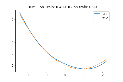
(a) $-1.5\cdot x+.9\cdot x^{2}$

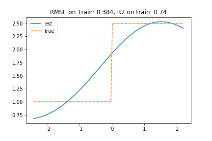
(b) $1+1.5\cdot 1\{x>0\}$

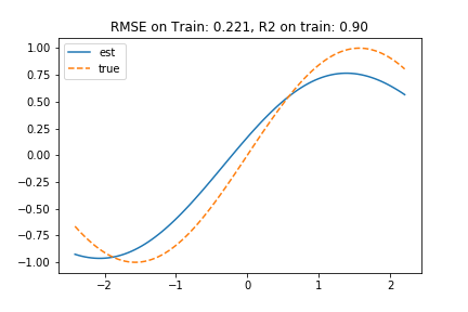
(c) $\sin(x)$

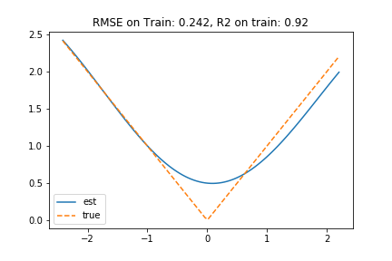
(d) $|x|$

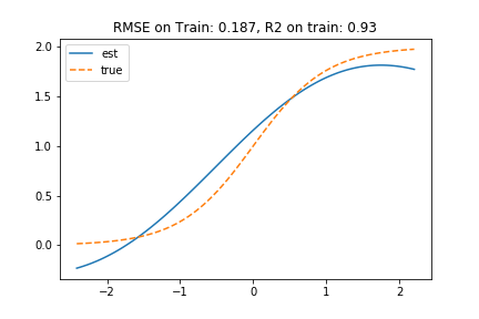
(e) $\frac{2}{1+e^{-2x}}$

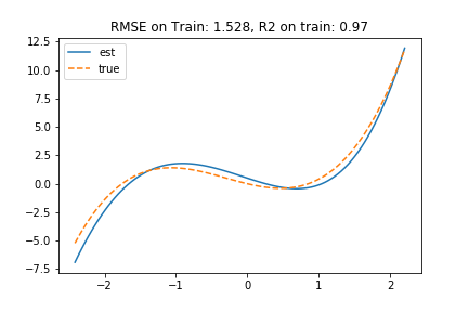
(f) $-1.5\cdot x+.9\cdot x^{2}+x^{3}$

Figure 5: Estimated functions based on our minimax estimator for different true functions. We use an rbf kernel with parameter $\gamma=.1$ and $1000$ samples. We chose critical radius parameter $\delta=5/n^{.4}$ and the regularization hyper-parameter $\tau$ is chosen via k-fold cross-validation. The data generating process was: $x=.6\,z+.4\,u+\delta$ and $y=h_{0}(x)+u+\epsilon$ and $z,u\sim N(0,2)$ and $\epsilon,\delta\sim N(0,.1)$.

Low-Rank Approximation and Nystrom’s Method

The solution to the empirical optimization problem requires inverting an $n\times n$ kernel matrix, which takes time $O(n^{3})$. This can be prohibitive for moderate sample sizes of the order of tens of thousands. We note here that one can construct very good approximations to the solution in Proposition 10 by considering low-rank approximations of the kernel matrix $K$. We present here one such low-rank approximation, based on Nystrom’s method, but we note that the plethora of recent literature on low-rank kernel approximation methods are applicable to our problem too (see e.g. Kumar et al. [2012], Bach and Jordan [2005], Musco and Musco [2017], Oglic and Gärtner [2017]).

Suppose that we can express our kernel matrices as $K_{{\mathcal{H}},n}$ and $K_{{\mathcal{H}},n}$ as $K_{{\mathcal{H}},n}=DD^{\top}$ and $K_{{\mathcal{H}},n}=VV^{\top}$, where $D$ and $V$ are of dimensions $n\times r$ and such that we can express the kernel row of any new test sample as:

$$(K_{\mathcal{H}}(x_{1},x),\ldots,K_{\mathcal{H}}(x_{n},x))=V\phi(x)$$ (78)

for some $r$-dimensional vector $\phi(x)$. Then we can express $h(x)=\phi(x)^{\top}V^{\top}a_{\lambda}$. If we then define $\gamma=V^{\top}\alpha_{\lambda}$. Then we can re-write the closed form solutions to the min and max problems as follows:

$$\sup_{f\in{\mathcal{F}}}\,\,\Psi_{n}(h,f)^{2}-\lambda\left(\|{f}\|_{K_{{\mathcal{F}}}}^{2}+\frac{U}{n\delta^{2}}\|f\|_{2,n}^{2}\right)=\frac{1}{4\lambda}\psi_{n}^{\top}D\left(\frac{U}{n\delta^{2}}D^{\top}D+I\right)^{-1}D^{\top}\psi_{n}$$ (79)

and if we let $Q:=\left(\frac{U}{n\delta^{2}}D^{\top}D+I\right)^{-1}$ and $A=V^{\top}D$, then:

$$\gamma:=~{} \left(AQA^{\top}+4\,\lambda\,\mu\,I\right)^{-1}AQD^{\top}y$$ (80)

$$\hat{h}(x):=~{} \phi(x)^{\top}\gamma$$ (81)

Observe that every matrix calculation in the above expressions requires time at most $O(n\,r^{2})$ to be computed. Thus if $r\ll n$, we have massively reduced the computation time from $\Theta(n^{3})$ to $O(n\,r^{2})$, making the method practical even very large data regimes.

Even though $r$ in the worst-case can be of size $n$, we can typically well-approximate the kernel matrices with $r\ll n$. One popular approach for achieving this is Nystrom’s method, which essentially sub-samples a set of $r$ points and uses the normalized kernel distances with respect to this subset of points as $D$ and $V$, respectively. In particular, let $S$ denote an $n\times r$ matrix whose $i$-th column contains a $1$ in position $j$ for some randomly sampled index $j$. Then $KS$ is an $n\times r$ sub-matrix of $K$, where a subset $S$ of the columns of $K$ are chosen at random. Then we can approximate $K$ via $VV^{\top}$, where $V=KSM^{1/2}$ and $M=(S^{\top}KS)^{+}$ (i.e. $V$ is contains normalized kernel-based similarities to the subset $S$ of $r$ randomly chosen points). Moreover, for any new test point, we can set $\phi(x)=M^{1/2}(K_{\mathcal{H}}(x_{i},x))_{i\in S}$.

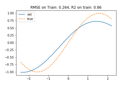
(a) $\sin(x)$

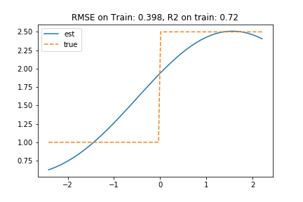
(b) $1+1.5\cdot 1\{x>0\}$

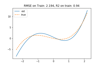
(c) $-1.5\cdot x+.9\cdot x^{2}+x^{3}$

Figure 6: Estimates based on Nystrom approximation, with $50$ nystrom samples, for the same dgp and parameter setup as in Figure 5.

E.4 Bounds on Ill-Posedness Measure

The results so far in the section provide bounds on the projected RMSE. In this last section, we show that under further assumptions on the strength of the instrument (i.e. the correlation of $x$ and $z$), then the projected RMSE rates also imply rates for the RMSE. We give an example such set of conditions, mostly as an example of a sufficient set of assumptions that lead to RMSE rates and in order to provide qualitative insights on what RMSE rates one can expect in different regimes of the instrument strength and the eigendecay of the kernel. In this section we will assume that the space ${\mathcal{H}}$ is also augmented with a hard constraint on the RKHS norm, i.e. ${\mathcal{H}}=\mathbb{H}_{K}^{B}=\{h\in\mathbb{H}_{K}:\|h\|_{K}\leq B\}$. Assuming $\|h_{0}\|_{K}\leq B$ this does not change the statistical guarantees and moreover the closed form optimization theorems, can easily be amended to incorporate a hard constraint on top of the regularization (due to the equivalent between hard constraints and regularization). Imposing this hard constraint will simplify the analysis of this section.

By Mercer’s theorem we can express any function in the RKHS $\mathbb{H}_{K}^{B}$, in terms of the eigenfunctions of the kernel:

$$h=\sum_{j\in J}a_{j}e_{j}$$ (82)

with $e_{j}:{\mathcal{X}}\to\mathbb{R}$, such that $\mathbb{E}[e_{j}(x)^{2}]=1$ and $\mathbb{E}[e_{i}(x)\,e_{j}(x)]=0$ and $J$ a countable set. Moreover, we have $\|h\|_{2}^{2}=\sum_{j\in J}a_{j}^{2}$ and $\|{h}\|_{K}=\sum_{j\in J}\frac{a_{j}^{2}}{\lambda_{j}}\leq B$. Thus we have that $\|h\|_{{\mathcal{H}}}^{2}\leq B$ implies that for all $m\in\mathbb{N}_{+}$: $\sum_{j\geq m}a_{j}^{2}\leq\lambda_{m}B$. Moreover, we have: [ ∥Th∥_2^2 = ∑_i, j∈J a_i a_j E[E[e_i(x)∣z]E[e_j(x)∣z]]. ]

For any $m\in\mathbb{N}_{+}$, let $I:=\{1,\ldots,m\}$, $e_{I}=(e_{1},\ldots,e_{m})$, $a_{I}=(a_{1},\ldots,a_{m})$ and:

$$V_{m}:=\mathbb{E}[\mathbb{E}[e_{I}(x)\mid z]\,\mathbb{E}[e_{I}(x)\mid z]^{\top}]$$ (83)

and suppose that $\lambda_{\min}(V_{m})\geq\tau_{m}$, i.e. that these finite eigenfunctions maintain some fraction of their independent components, even when they are smoothened through the conditional expectation $p(x\mid z)$. Furthermore suppose that for all $i\leq m<j$: $\left|\mathbb{E}[\mathbb{E}[e_{i}(x)\mid z]\mathbb{E}[e_{j}(x)\mid z]]\right|\leq\gamma_{m}\leq c\,\tau_{m}$ (for some constant $c$), i.e. the smoothening performed by the conditional expectation does not ruin a lot the orthogonality of the first $m$ eigenfunctions with eigenfunctions for indices larger than $m$. Observe that if we had a perfect instrument, i.e. $z$ was perfectly correlated with $x$, then $V_{m}=I_{m}$ and $\mathbb{E}[\mathbb{E}[e_{i}(x)\mid z]\mathbb{E}[e_{j}(x)\mid z]]=\mathbb{E}[e_{i}(x)e_{j}(x)]=0$. Thus for a perfect instrument $\tau_{m}=1$ and $\gamma_{m}=0$. Therefore the latter requirements are implicit assumptions on the strength of the instrument. We show that under these assumptions, we can bound the measure of ill-posedness as follows.

Lemma 11.

Suppose that $\lambda_{\min}(V_{m})\geq\tau_{m}$ and for some constant $c>0$, for all $i\leq m<j$,

References

- Agarwal et al. [2014] Alekh Agarwal, Olivier Chapelle, Miroslav Dudík, and John Langford. A reliable effective terascale linear learning system. The Journal of Machine Learning Research, 15(1):1111–1133, 2014.
- Allen-Zhu et al. [2018] Zeyuan Allen-Zhu, Yuanzhi Li, and Yingyu Liang. Learning and Generalization in Overparameterized Neural Networks, Going Beyond Two Layers. arXiv e-prints, art. arXiv:1811.04918, November 2018.
- Anthony and Bartlett [2009] Martin Anthony and Peter L Bartlett. Neural network learning: Theoretical foundations. cambridge university press, 2009.
- Bach and Jordan [2005] Francis R Bach and Michael I Jordan. Predictive low-rank decomposition for kernel methods. In Proceedings of the 22nd international conference on Machine learning, pages 33–40, 2005.
- Balasubramanian et al. [2017] Krishnakumar Balasubramanian, Tong Li, and Ming Yuan. On the optimality of kernel-embedding based goodness-of-fit tests. arXiv preprint arXiv:1709.08148, 2017.
- Bartlett et al. [2005] Peter L Bartlett, Olivier Bousquet, Shahar Mendelson, et al. Local rademacher complexities. The Annals of Statistics, 33(4):1497–1537, 2005.
- Bartlett et al. [2017] Peter L Bartlett, Dylan J Foster, and Matus J Telgarsky. Spectrally-normalized margin bounds for neural networks. In Advances in Neural Information Processing Systems, pages 6240–6249, 2017.
- Bennett et al. [2019] Andrew Bennett, Nathan Kallus, and Tobias Schnabel. Deep generalized method of moments for instrumental variable analysis. In Advances in Neural Information Processing Systems, pages 3559–3569, 2019.
- Binkowski et al. [2018] Mikolaj Binkowski, Dougal J. Sutherland, Michael Arbel, and Arthur Gretton. Demystifying MMD GANs. In International Conference on Learning Representations, 2018.
- Blundell et al. [2007] Richard Blundell, Xiaohong Chen, and Dennis Kristensen. Semi-nonparametric iv estimation of shape-invariant engel curves. Econometrica, 75(6):1613–1669, 2007.
- Bottou et al. [2007] Léon Bottou, Olivier Chapelle, Dennis DeCoste, and Jason Weston. Large-Scale Kernel Machines (Neural Information Processing). The MIT Press, 2007. ISBN 0262026252.
- Boyd and Vandenberghe [2004] Stephen Boyd and Lieven Vandenberghe. Convex optimization. Cambridge University Press, 2004.
- Bronshtein [1976] EM Bronshtein. -entropy of convex sets and functions. Siberian Mathematical Journal, 17(3):393–398, 1976.
- Caponnetto and De Vito [2007] Andrea Caponnetto and Ernesto De Vito. Optimal rates for the regularized least-squares algorithm. Foundations of Computational Mathematics, 7(3):331–368, 2007.
- Chatterjee et al. [2015] Sabyasachi Chatterjee, Adityanand Guntuboyina, and Bodhisattva Sen. On risk bounds in isotonic and other shape restricted regression problems. Ann. Statist., 43(4):1774–1800, 08 2015. doi: 10.1214/15-AOS1324. URL https://doi.org/10.1214/15-AOS1324.
- Chen and Christensen [2018] Xiaohong Chen and Timothy M Christensen. Optimal sup-norm rates and uniform inference on nonlinear functionals of nonparametric iv regression. Quantitative Economics, 9(1):39–84, 2018.
- Chen and Pouzo [2009] Xiaohong Chen and Demian Pouzo. Efficient estimation of semiparametric conditional moment models with possibly nonsmooth residuals. Journal of Econometrics, 152(1):46–60, 2009.
- Chen and Pouzo [2012] Xiaohong Chen and Demian Pouzo. Estimation of nonparametric conditional moment models with possibly nonsmooth generalized residuals. Econometrica, 80(1):277–321, 2012.
- Chernozhukov et al. [2018] Victor Chernozhukov, Denis Chetverikov, Mert Demirer, Esther Duflo, Christian Hansen, Whitney Newey, and James Robins. Double/debiased machine learning for treatment and structural parameters. The Econometrics Journal, 21(1):C1–C68, 2018. doi: 10.1111/ectj.12097. URL https://onlinelibrary.wiley.com/doi/abs/10.1111/ectj.12097.
- Chetverikov and Wilhelm [2017] Denis Chetverikov and Daniel Wilhelm. Nonparametric instrumental variable estimation under monotonicity. Econometrica, 85(4):1303–1320, 2017. doi: 10.3982/ECTA13639. URL https://onlinelibrary.wiley.com/doi/abs/10.3982/ECTA13639.
- Darolles et al. [2011] Serge Darolles, Yanqin Fan, Jean-Pierre Florens, and Eric Renault. Nonparametric instrumental regression. Econometrica, 79(5):1541–1565, 2011.
- Daskalakis et al. [2017] Constantinos Daskalakis, Andrew Ilyas, Vasilis Syrgkanis, and Haoyang Zeng. Training gans with optimism. CoRR, abs/1711.00141, 2017. URL http://arxiv.org/abs/1711.00141.
- del Álamo and Munk [2019] Miguel del Álamo and Axel Munk. Total variation multiscale estimators for linear inverse problems. arXiv preprint arXiv:1905.08515, 2019.
- Du et al. [2018] Simon S Du, Xiyu Zhai, Barnabas Poczos, and Aarti Singh. Gradient descent provably optimizes over-parameterized neural networks. arXiv preprint arXiv:1810.02054, 2018.
- Duchi and Singer [2009] John Duchi and Yoram Singer. Efficient online and batch learning using forward backward splitting. Journal of Machine Learning Research, 10(99):2899–2934, 2009. URL http://jmlr.org/papers/v10/duchi09a.html.
- Duchi et al. [2008] John Duchi, Shai Shalev-Shwartz, Yoram Singer, and Tushar Chandra. Efficient projections onto the l1-ball for learning in high dimensions. In Proceedings of the 25th International Conference on Machine Learning, ICML08, pages 272–279, New York, NY, USA, 2008. doi: 10.1145/1390156.1390191.
- Fan and Liao [2014] Jianqing Fan and Yuan Liao. Endogeneity in high dimensions. Annals of statistics, 42(3):872, 2014.
- Foster and Syrgkanis [2019] Dylan J. Foster and Vasilis Syrgkanis. Orthogonal Statistical Learning. arXiv e-prints, art. arXiv:1901.09036, January 2019.
- Freund and Schapire [1999] Yoav Freund and Robert E. Schapire. Adaptive game playing using multiplicative weights. Games and Economic Behavior, 29(1):79 – 103, 1999. ISSN 0899-8256. doi: https://doi.org/10.1006/game.1999.0738. URL http://www.sciencedirect.com/science/article/pii/S0899825699907388.
- Gautier et al. [2011] Eric Gautier, Alexandre Tsybakov, and Christiern Rose. High-dimensional instrumental variables regression and confidence sets. arXiv preprint arXiv:1105.2454, 2011.
- Gine and Nickl [2015] Evarist Gine and Richard Nickl. Mathematical Foundations of Infinite-Dimensional Statistical Models. Cambridge University Press, USA, 1st edition, 2015. ISBN 1107043166.
- Golowich et al. [2018] Noah Golowich, Alexander Rakhlin, and Ohad Shamir. Size-independent sample complexity of neural networks. In Sébastien Bubeck, Vianney Perchet, and Philippe Rigollet, editors, Proceedings of the 31st Conference On Learning Theory, volume 75 of Proceedings of Machine Learning Research, pages 297–299. PMLR, 06–09 Jul 2018. URL http://proceedings.mlr.press/v75/golowich18a.html.
- Guntuboyina and Sen [2012] Adityanand Guntuboyina and Bodhisattva Sen. Covering numbers for convex functions. IEEE Transactions on Information Theory, 59(4):1957–1965, 2012.
- Hall et al. [2005] Peter Hall, Joel L Horowitz, et al. Nonparametric methods for inference in the presence of instrumental variables. The Annals of Statistics, 33(6):2904–2929, 2005.
- Hansen [1982] Lars Peter Hansen. Large sample properties of generalized method of moments estimators. Econometrica, 50(4):1029–1054, 1982. ISSN 00129682, 14680262. URL http://www.jstor.org/stable/1912775.
- Hartford et al. [2017] Jason Hartford, Greg Lewis, Kevin Leyton-Brown, and Matt Taddy. Deep IV: A flexible approach for counterfactual prediction. In Doina Precup and Yee Whye Teh, editors, Proceedings of the 34th International Conference on Machine Learning, volume 70 of Proceedings of Machine Learning Research, pages 1414–1423, International Convention Centre, Sydney, Australia, 06–11 Aug 2017. PMLR. URL http://proceedings.mlr.press/v70/hartford17a.html.
- Horowitz [2007] Joel L Horowitz. Asymptotic normality of a nonparametric instrumental variables estimator. International Economic Review, 48(4):1329–1349, 2007.
- Horowitz [2011] Joel L Horowitz. Applied nonparametric instrumental variables estimation. Econometrica, 79(2):347–394, 2011.
- Hsieh et al. [2019] Yu-Guan Hsieh, Franck Iutzeler, Jérôme Malick, and Panayotis Mertikopoulos. On the convergence of single-call stochastic extra-gradient methods. arXiv e-prints, art. arXiv:1908.08465, August 2019.
- Jin et al. [2019] Chi Jin, Praneeth Netrapalli, and Michael I. Jordan. Minmax optimization: Stable limit points of gradient descent ascent are locally optimal. CoRR, abs/1902.00618, 2019. URL http://arxiv.org/abs/1902.00618.
- Kakade et al. [2011] Sham M Kakade, Varun Kanade, Ohad Shamir, and Adam Kalai. Efficient learning of generalized linear and single index models with isotonic regression. In J. Shawe-Taylor, R. S. Zemel, P. L. Bartlett, F. Pereira, and K. Q. Weinberger, editors, Advances in Neural Information Processing Systems 24, pages 927–935. Curran Associates, Inc., 2011.
- Kumar et al. [2012] Sanjiv Kumar, Mehryar Mohri, and Ameet Talwalkar. Sampling methods for the nyström method. Journal of Machine Learning Research, 13(Apr):981–1006, 2012.
- Langford et al. [2009] John Langford, Lihong Li, and Tong Zhang. Sparse online learning via truncated gradient. In D. Koller, D. Schuurmans, Y. Bengio, and L. Bottou, editors, Advances in Neural Information Processing Systems 21, pages 905–912. Curran Associates, Inc., 2009.
- Le [2013] Quoc V Le. Building high-level features using large scale unsupervised learning. In 2013 IEEE international conference on acoustics, speech and signal processing, pages 8595–8598. IEEE, 2013.
- Lecué and Mendelson [2017] Guillaume Lecué and Shahar Mendelson. Regularization and the small-ball method ii: complexity dependent error rates. The Journal of Machine Learning Research, 18(1):5356–5403, 2017.
- Lecué and Mendelson [2018] Guillaume Lecué and Shahar Mendelson. Regularization and the small-ball method i: Sparse recovery. Ann. Statist., 46(2):611–641, 04 2018. doi: 10.1214/17-AOS1562. URL https://doi.org/10.1214/17-AOS1562.
- Lei et al. [2019] Qi Lei, Jason D. Lee, Alexandros G. Dimakis, and Constantinos Daskalakis. SGD Learns One-Layer Networks in WGANs. arXiv e-prints, art. arXiv:1910.07030, October 2019.
- Li et al. [2017] Chun-Liang Li, Wei-Cheng Chang, Yu Cheng, Yiming Yang, and Barnabás Póczos. Mmd gan: Towards deeper understanding of moment matching network. In Advances in Neural Information Processing Systems, pages 2203–2213, 2017.
- Lin et al. [2020] Tianyi Lin, Chi Jin, Michael Jordan, et al. Near-optimal algorithms for minimax optimization. arXiv preprint arXiv:2002.02417, 2020.
- Liu et al. [2020] Feng Liu, Wenkai Xu, Jie Lu, Guangquan Zhang, Arthur Gretton, and DJ Sutherland. Learning deep kernels for non-parametric two-sample tests. arXiv preprint arXiv:2002.09116, 2020.
- Mansour and McAllester [2000] Yishay Mansour and David A. McAllester. Generalization bounds for decision trees. In Proceedings of the Thirteenth Annual Conference on Computational Learning Theory, COLT00, pages 69–74, San Francisco, CA, USA, 2000. Morgan Kaufmann Publishers Inc. ISBN 155860703X.
- Massart [2000] Pascal Massart. Some applications of concentration inequalities to statistics. Annales de la Faculté des sciences de Toulouse : Mathématiques, Ser. 6, 9(2):245–303, 2000. URL http://www.numdam.org/item/AFST_2000_6_9_2_245_0.
- Maurer [2016] Andreas Maurer. A vector-contraction inequality for rademacher complexities. In International Conference on Algorithmic Learning Theory, pages 3–17. Springer, 2016.
- McMahan [2011] Brendan McMahan. Follow-the-regularized-leader and mirror descent: Equivalence theorems and l1 regularization. In Proceedings of the Fourteenth International Conference on Artificial Intelligence and Statistics, pages 525–533, 2011.
- Mertikopoulos et al. [2018] Panayotis Mertikopoulos, Houssam Zenati, Bruno Lecouat, Chuan-Sheng Foo, Vijay Chandrasekhar, and Georgios Piliouras. Mirror descent in saddle-point problems: Going the extra (gradient) mile. CoRR, abs/1807.02629, 2018. URL http://arxiv.org/abs/1807.02629.
- Mishchenko et al. [2019] Konstantin Mishchenko, Dmitry Kovalev, Egor Shulgin, Peter Richtárik, and Yura Malitsky. Revisiting Stochastic Extragradient. arXiv e-prints, art. arXiv:1905.11373, May 2019.
- Mokhtari et al. [2019] Aryan Mokhtari, Asuman Ozdaglar, and Sarath Pattathil. A unified analysis of extra-gradient and optimistic gradient methods for saddle point problems: Proximal point approach. arXiv preprint arXiv:1901.08511, 2019.
- Muandet et al. [2019] Krikamol Muandet, Arash Mehrjou, Si Kai Lee, and Anant Raj. Dual iv: A single stage instrumental variable regression. arXiv preprint arXiv:1910.12358, 2019.
- Muandet et al. [2020] Krikamol Muandet, Wittawat Jitkrittum, and Jonas Kübler. Kernel conditional moment test via maximum moment restriction. arXiv preprint arXiv:2002.09225, 2020.
- Musco and Musco [2017] Cameron Musco and Christopher Musco. Recursive sampling for the nystrom method. In Advances in Neural Information Processing Systems, pages 3833–3845, 2017.
- Negahban et al. [2012] Sahand N. Negahban, Pradeep Ravikumar, Martin J. Wainwright, and Bin Yu. A unified framework for high-dimensional analysis of -estimators with decomposable regularizers. Statist. Sci., 27(4):538–557, 11 2012. doi: 10.1214/12-STS400. URL https://doi.org/10.1214/12-STS400.
- Nemirovski [2004] Arkadi Nemirovski. Prox-method with rate of convergence o(1/t) for variational inequalities with lipschitz continuous monotone operators and smooth convex-concave saddle point problems. SIAM Journal on Optimization, 15(1):229–251, 2004. doi: 10.1137/S1052623403425629. URL https://doi.org/10.1137/S1052623403425629.
- Nesterov [2005] Yu Nesterov. Smooth minimization of non-smooth functions. Mathematical programming, 103(1):127–152, 2005.
- Newey and Powell [2003] Whitney K Newey and James L Powell. Instrumental variable estimation of nonparametric models. Econometrica, 71(5):1565–1578, 2003.
- Nouiehed et al. [2019] Maher Nouiehed, Maziar Sanjabi, Tianjian Huang, Jason D Lee, and Meisam Razaviyayn. Solving a class of non-convex min-max games using iterative first order methods. In Advances in Neural Information Processing Systems 32, pages 14934–14942. Curran Associates, Inc., 2019.
- Oglic and Gärtner [2017] Dino Oglic and Thomas Gärtner. Nyström method with kernel k-means++ samples as landmarks. In Proceedings of the 34th International Conference on Machine Learning-Volume 70, pages 2652–2660. JMLR. org, 2017.
- Rahimi and Recht [2008] Ali Rahimi and Benjamin Recht. Random features for large-scale kernel machines. In Advances in neural information processing systems, pages 1177–1184, 2008.
- Rakhlin et al. [2017] Alexander Rakhlin, Karthik Sridharan, and Alexandre B. Tsybakov. Empirical entropy, minimax regret and minimax risk. Bernoulli, 23(2):789–824, 05 2017. doi: 10.3150/14-BEJ679. URL https://doi.org/10.3150/14-BEJ679.
- Rakhlin and Sridharan [2013] Sasha Rakhlin and Karthik Sridharan. Optimization, learning, and games with predictable sequences. In C. J. C. Burges, L. Bottou, M. Welling, Z. Ghahramani, and K. Q. Weinberger, editors, Advances in Neural Information Processing Systems 26, pages 3066–3074. Curran Associates, Inc., 2013.
- Schölkopf et al. [2001] Bernhard Schölkopf, Ralf Herbrich, and Alex J Smola. A generalized representer theorem. In International conference on computational learning theory, pages 416–426. Springer, 2001.
- Shalev-Shwartz and Ben-David [2014] Shai Shalev-Shwartz and Shai Ben-David. Understanding machine learning: From theory to algorithms. Cambridge university press, 2014.
- Shalev-Shwartz and Singer [2007] Shai Shalev-Shwartz and Yoram Singer. Convex repeated games and fenchel duality. In Advances in neural information processing systems, pages 1265–1272, 2007.
- Singh et al. [2019] Rahul Singh, Maneesh Sahani, and Arthur Gretton. Kernel instrumental variable regression. In Advances in Neural Information Processing Systems, pages 4595–4607, 2019.
- Soltanolkotabi et al. [2019] M. Soltanolkotabi, A. Javanmard, and J. D. Lee. Theoretical insights into the optimization landscape of over-parameterized shallow neural networks. IEEE Transactions on Information Theory, 65(2):742–769, 2019.
- Sra et al. [2012] Suvrit Sra, Sebastian Nowozin, and Stephen J Wright. Optimization for machine learning. Mit Press, 2012.
- Syrgkanis et al. [2015] Vasilis Syrgkanis, Alekh Agarwal, Haipeng Luo, and Robert E Schapire. Fast convergence of regularized learning in games. In Advances in Neural Information Processing Systems, pages 2989–2997, 2015.
- Thekumparampil et al. [2019] Kiran K Thekumparampil, Prateek Jain, Praneeth Netrapalli, and Sewoong Oh. Efficient algorithms for smooth minimax optimization. In Advances in Neural Information Processing Systems 32, pages 12680–12691. Curran Associates, Inc., 2019.
- Vaart and Wellner [1996] A. W. Van Der Vaart and J. A. Wellner. Weak Convergence and Empirical Processes: With Applications to Statistics. Springer Series, March 1996.
- Wainwright [2019] Martin J Wainwright. High-dimensional statistics: A non-asymptotic viewpoint, volume 48. Cambridge University Press, 2019.
- Wendland [2004] Holger Wendland. Scattered data approximation, volume 17. Cambridge university press, 2004.
- Yang et al. [2020] Junchi Yang, Negar Kiyavash, and Niao He. Global convergence and variance-reduced optimization for a class of nonconvex-nonconcave minimax problems. arXiv preprint arXiv:2002.09621, 2020.
- Yeganova and Wilbur [2009] L. Yeganova and W. J. Wilbur. Isotonic regression under lipschitz constraint. Journal of Optimization Theory and Applications, 141(2):429–443, 2009. doi: 10.1007/s10957-008-9477-0. URL https://doi.org/10.1007/s10957-008-9477-0.
- Zhang et al. [2014] Yuchen Zhang, Martin J Wainwright, and Michael I Jordan. Lower bounds on the performance of polynomial-time algorithms for sparse linear regression. In Conference on Learning Theory, pages 921–948, 2014.