Classical and quantum vortex leapfrogging in two-dimensional channels

Abstract

The leapfrogging of coaxial vortex rings is a famous effect which has been noticed since the times of Helmholtz. Recent advances in ultra-cold atomic gases show that the effect can now be studied in quantum fluids. The strong confinement which characterizes these systems motivates the study of leapfrogging of vortices within narrow channels. Using the two-dimensional point vortex model, we show that in the constrained geometry of a two-dimensional channel the dynamics is richer than in an unbounded domain: alongsize the known regimes of standard leapfrogging and the absence of it, we identify new regimes of backward leapfrogging and periodic orbits. Moreover, by solving the Gross-Pitaevskii equation for a Bose-Einstein condensate, we show that all four regimes exist for quantum vortices too. Finally, we discuss the differences between classical and quantum vortex leapfrogging which appear when the quantum healing length becomes significant compared to the vortex separation or the channel size, and when, due to high velocity, compressibility effects in the condensate becomes significant.

I Introduction

The leapfrogging of two co-axial vortex rings (in three dimensions) or of two vortex-antivortex pairs (in two dimensions) is a benchmark problem of vortex interaction (Meleshko, 2010) which dates back to (Helmholtz, 1858). The time evolution of this vortex configuration is striking: the vortex ring (or pair) which is ahead widens and slows down, while the ring behind contracts, speeds up, catches up with the first ring and goes ahead through it; this ‘leapfrogging’ game is then repeated over and over again, unless instabilities disrupt it. A number of papers have been written on different aspects of this problem, ranging from the stability (Hicks, 1922; Love, 1894; Acheson, 2000; Tophøj & Aref, 2013) to the deformation of the vortex cores and to the effects of viscosity (Shariff & Leonard, 1992) using numerical (Riley & Stevens, 1993; Borisov, 2014; Cheng & Lim, 2015) as well as experimental methods (Maxworthy, 1972; Yamada & Matsui, 1978; Lim, 1997; Qin et al., 2018). The most recent developments concern leapfrogging of vortex bundles (Wacks et al., 2014) and helical waves (Hietala et al., 2016; Selçuk et al., 2018; Quaranta et al., 2019).

Our work is motivated by recent experiments with atomic Bose-Einstein condensates, which constitute a dilute quantum fluid and provide an idealised platform to study fundamental vortex dynamics (White et al., 2014). In these experiments, atomic gases are confined by suitable magnetic-optical traps and cooled to nano-Kelvin temperatures. If the atoms of the gas are bosons (i.e. have integer spin), a phase transition occurs upon cooling below a critical temperature $T_{c}$, and the gas forms a macroscopic coherent quantum state (Barenghi & Parker, 2016) called a Bose-Einstein condensate (BEC). From the point of view of the hydrodynamics, a BEC has three key properties: it is superfluid (i.e. it suffers no viscous losses of kinetic energy when it flows), it is compressible, and its vorticity is concentrated to thin hollow vortex lines with fixed width $a_{0}$ and fixed circulation $\pm h/m$ where $h$ is Planck’s constant and $m$ is the mass of a boson (while vortices with larger quanta of circulation, $\pm 2h/m,\pm 3h/m,\cdots$, are possible, they are unstable to decay into multiple singly-charged vortices). Thus, in BECs, vortices are well-defined and identical objects, evolving in an inviscid compressible fluid.

There are several additional characteristics of atomic BECs that make them attractive for probing vortex dynamics. Firstly, the physical parameters of the fluid (including the width and speed of the vortices) are tunable, for example, through the density of the gas and the strength of the atom-atom interaction (which can be modified by means of Feshbach resonances (Inouye et al., 1998)); this should be contrasted with superfluid liquid helium - historically the most studied quantum fluid - whose physical parameters are fixed by nature. Secondly, the potential experienced by the gas can be controlled through magnetic and optical fields. Such trapping is essential, on one hand, to contain the gas, and gives rise to the boundary effects which are central to this work. However, the potential can also be exploited to engineer the dimensionality of the gas - particularly, quasi-two-dimensional geometries in which vortex lines effectively become point-like vortices - and to stir and shake the condensate. Finally, recent techniques have enabled the observation of vortex lines (Serafini et al., 2017) and vortex points (Seo et al., 2017) in real-time, including inference of their individual circulations.

Atomic BECs have been employed as a context to study a range of fundamental vortex phenomena, including vortex nucleation from moving obstacles (Frisch et al., 1992; Nore et al., 1993; Neely et al., 2010; Stagg et al., 2014; Kwon et al., 2015) and flow constriction (Valtolina et al., 2015; Burchianti et al., 2018; Xhani et al., 2020), von Kármán vortex streets (Sasaki et al., 2010; Kwon et al., 2016), vortex-antivortex annihilations (Seo et al., 2017), vortex line reconnections (Serafini et al., 2017; Galantucci et al., 2019), vortex chaos (Navarro et al., 2013), vortex scattering (Barenghi el al., 2005; Caplan et al., 2014; Griffin et al., 2017), quantum turbulence (Henn et al., 2009; Neely et al., 2013; Kwon et al., 2014; Stagg et al., 2015; White et al., 2014; Tsatsos et al., 2016; Garcia-Orozco et al., 2020), and self-organisation and clustering of vortices (Simula et al., 2014; Billam et al., 2014; Gauthier et al., 2019; Johnstone et al., 2019). With regards to vortex leapfrogging, this has been considered theoretically in idealised unconfined condensates (Ikuta et al., 2019), including spinor condensates (Kaneda & Saito, 2014).

Atomic BECs however are characterized by their small dimensions, typically from 10 to 100 times the vortex core size, for which the motion of vortices can be significantly affected by the presence of boundaries. This drawback is mainly due to the loss of atoms in the final evaporative stage of cooling the gas. There are even experiments in which, by design, the most interesting physics occurs in the most restricted region of the system, for example vortex rings nucleated in the weak link of the Josephson junction between two condensates (Valtolina et al., 2015; Xhani et al., 2020). The aim of the present work is to provide insight in the interpretation of current and future experimental studies of vortex dynamics in confined condensates (rather than idealised open domains), where leapfrogging dynamics, which can be established if the vortex nucleation frequency is sufficiently high, is affected by the presence of boundaries. The characteristics of leapfrogging motion in such confined systems is likely to show significant dissimilarities compared to the corresponding dynamics in unbounded systems stemming from the role played by image vortices arising from the presence of boundaries. Despite the expected impact of geometrical confinement, to the best of our knowledge the role of boundaries in leapfrogging dynamics has never been investigated in literature neither for classical nor for quantum fluids ((Kaneda & Saito, 2014) and (Ikuta et al., 2019) indeed studied leapfrogging in homogeneous condensates, without boundaries). In order to assess the impact of the boundaries and disentangle the latter from other concurrent physical effects existing in quantum fluids (e.g. compressibility), in this research we compare the leapfrogging of vortices in plane channels in (i) ideal incompressible classical fluids and (ii) box-trapped Bose-Einstein condensates. In order to simplify the system under investigation, our theoretical and numerical analysis is performed in two-dimensions, employing the point vortex model for classical fluids and the Gross-Pitaevskii equation for BECs. We stress that the Gross-Pitaevskii equation has proved an excellent quantitative model of experiments with Bose-Einstein condensates at temperatures $T\ll T_{c}$; at relatively high values of temperature, the condensate exchanges energy and particles with the thermal cloud, and the Gross-Pitaevskii equation requires modifications (Breczyk et al., 2007; Proukakis & Jackson, 2008; Blakie et al., 2014; Berloff et al., 2014). We also remark that on one hand the two-dimensional nature of the system that we consider is an idealisation (the aim is to get insight in the motion of three-dimensional vortex rings), but, on the other hand, where atomic Bose-Einstein condensates are tightly confined in one direction the system becomes effectively two-dimensional and our two-dimensional approach becomes realistic.

The article is organised as follows. In Section II, we illustrate the two theoretical models employed, namely the classical point vortex model and the Gross-Pitaevskii equation describing the dynamics of BECs in the zero-temperature limit. In Section III, we report the results obtained in both classical and quantum fluids, focusing on the role of boundaries and on the differences between classical and quantum systems. Finally, in the last Section IV, we summarise our findings and illustrate their importance in the future of quantum vortex experiments.

II Models

II.1 Point vortex model

The simplest model of our system is the classical point vortex model: a two-dimensional inviscid incompressible irrotational fluid in an infinite channel of width $2D$ containing two vortex-antivortex pairs (the two-dimensional analog of three-dimensional coaxial vortex rings), each of circulation $\pm\Gamma$. In view of comparing the results obtained with this classical model to quantum vortices in confined BECs, the hypotheses behind the point vortex model must be carefully considered.

The classical model describes a fluid with constant density. In the bulk of the condensate, i.e. sufficiently far from boundaries or vortices, this assumption is realistic: indeed, although in past experiments condensates were usually confined by harmonic trapping potentials resulting in density gradients (Dalfovo et al., 1999), current experimental techniques (Gaunt et al., 2013) allow box-like trapping potentials which lead to uniform density profiles in the bulk of the condensate as in the classical point vortex model. In particular, in the vicinity of a vortex, the classical model assumes constant density at any radial distance $r$ to the vortex axis, including the vortex axis $r=0$ itself. In Bose-Einstein condensates, a vortex is a topological defect of the phase of the governing complex wavefunction (or order parameter), as we shall describe with more details in Section II.2.1. Therefore the vortex core is a thin tubular region around the vortex axis which is depleted of atoms: as $r\rightarrow 0$, the velocity tends to infinity, as in the point vortex model, but the fluid density tends to zero. The radius of this tube is of the order of the quantum mechanical healing length $\xi$ (see Section II.2.1). A similar difference between the classical point vortex model and Bose-Einstein condensates occurs near a hard boundary: the classical model assumes that the fluid’s density is constant up to the boundary; in a Bose-Einstein condensate a thin boundary region (again of the order of $\xi$) forms near the boundary where, in the case of box-like traps, the condensate’s density rapidly drops from the bulk value to zero. We conclude that, from a geometrical point of view, the classical point vortex model can be used to model Bose-Einstein condensates provided that vortex-vortex and vortex-boundary distances are larger than the healing length $\xi$.

From a dynamical point of view, the assumption of constant density implies that the classical point vortex model neglects sound waves which are radiated away by quantum vortices when they accelerate (Barenghi el al., 2005). The point vortex model, in fact, is based on the classical ideal Euler equation which conserves energy. In the low temperature limit $T/T_{c}\ll 1$ that guarantees the validity of the Gross-Pitaevskii equation, the total energy of a BEC is constant, but transformation of incompressible kinetic energy of the vortex configuration into compressible kinetic energy of the field of sound waves (or vice versa) is permitted. This dynamical difference between the classical point vortex model and the Gross-Pitaevskii model is, physically, perhaps the most significant, and will be addressed while discussing the results in Section III.

Despite these approximations, we reckon the model captures the essential ingredient of our problem: the motion of quantised irrotational vortices in presence of boundaries. Indeed, the classical point vortex model in a circular disk has been already used with success to model two-dimensional turbulence in low temperature trapped condensates, for example, by Simula et al. (2014). It must also be noticed that Mason et al. (2006) have shown that the motion of a realistic vortex at distance $d$ to a boundary can be described in terms of a classical image vortex even if $\xi$ is comparable to $d$ (although a small correction is needed to account for the density depletion in the boundary region). In the suitable physical limits, we hence expect the point vortex model to correctly describe the impact of boundaries on the leapfrogging of quantised vortices.

II.1.1 Equations of motion

Our physical domain under investigation is a two-dimensional infinite strip $\mathcal{C}_{\mathbb{R}^{2}}$ defined as $\mathcal{C}_{\mathbb{R}^{2}}=\{(x,y)\in\mathbb{R}^{2}\;\;:\;\;(x,y)\in\left(-\infty,\infty\right)\times\left(0,2D\right)\}$, which hereafter we will refer to as the channel. We assume the flow to be two-dimensional, i.e. the velocity vertical component $v_{z}=0$ and the horizontal components $v_{x}$ and $v_{y}$ only depend on horizontal coordinates $x$ and $y$ and time $t$. The incompressibility assumption implies that the continuity equation can be written as follows

$$\nabla\cdot\mathbf{v}=0.$$ (1)

The velocity field $\mathbf{v}$ can hence be expressed as the curl of vector field $\displaystyle\bm{\Psi}$ which, given the two-dimensionality of the flow, has non-vanishing components only in the $z$ direction, $\displaystyle\bm{\Psi}=(0,0,\psi(x,y,t))$. The velocity components have hence the following expressions in terms of the function $\psi$ which is often denominated streamfunction: $v_{x}~{}=~{}\partial_{y}\psi$ and $v_{y}~{}=~{}-\partial_{x}\psi$, where $\partial_{i}$ indicates spatial derivatives in the $i$ direction.

The irrotationality of the flow implies that the velocity field can be expressed via a potential function $\varphi$, i.e.

$$\mathbf{v}=\nabla\varphi\;\;,$$ (2)

leading to the following relations for the components $v_{i}=\partial_{i}\varphi$. Equations (1) and (2) imply that both $\varphi$ and $\psi$ satisfy Laplace equation, $\Delta\varphi=\Delta\psi=0$, and the following equalities between their spatial derivatives:

$$\displaystyle\partial_{x}\varphi = \partial_{y}\psi\;\;,$$ (3)

$$\partial_{y}\varphi = -\partial_{x}\psi.$$ (4)

Equations (3) and (4) coincide with the well known Cauchy-Riemann relations for the complex function $\Omega(z):=\varphi+\rm i\psi$, where $z=x+iy$. Hence, following basic complex analysis, the function $\Omega(z)$, denominated complex potential, is an analytical complex function on the simply connected open domain $\mathcal{C}=\{z\;\in\;\mathbb{C}\;:\;0<\Im\rm m\;z<2D\}\subsetneq\mathbb{C}$. As a consequence, $\Omega(z)$ is differentiable and its derivative

$$w(z):=\frac{d\Omega}{dz}=v_{x}-iv_{y}$$ (5)

is the so-called complex velocity. In the framework of complex potentials, the impermeable boundary conditions for ideal fluids correspond in our channel $\mathcal{C}$ to the following constraint: $\Im\text{m}\;\Omega(z)_{\arrowvert_{z\in\partial\mathcal{C}}}=\alpha(t)$, with $\alpha(t)\in\mathbb{R}$ depending only on time $t$.

The description of incompressible and irrotational flows of ideal fluids via the complex potential-based formulation is particularly useful in the present work as it allows the employment of conformal mapping techniques for the derivation of the analytical expression of the complex potential $\Omega(z)$ describing the velocity field induced by a point vortex in our channel $\mathcal{C}$. The essential steps for this derivation are as follows. The necessary ingredients are mainly two: (a) the knowledge of the complex potential $\Theta(\zeta)$ describing the flow induced by a point vortex in a simply connected open subset $\mathcal{D}$ of the complex plane, with $\zeta\in\mathcal{D}\subsetneq\mathbb{C}$; and (b) the construction of a conformal map $\zeta=f(z)$ transforming our channel $\mathcal{C}$ onto the domain $\mathcal{D}$.

Conformal maps $f$ are transformations defined on the complex plane which preserve angles. Such maps are performed by analytical complex functions with non-vanishing derivative, i.e., in the present case, $f^{\prime}(z)\neq 0$ for all $z\in\mathcal{C}$. The requirement $\mathcal{D}$ not coinciding with the entire complex plane $\mathbb{C}$, is fundamental in order to exploit the Riemann Mapping Theorem which ensures the existence of the conformal map $f$ mapping $\mathcal{C}$ onto $\mathcal{D}$. Once $\Theta(\zeta)$ and $f(z)$ are determined, the complex potential $\Omega(z)$ for a vortex flow in $\mathcal{C}$ is obtained by transforming the potential $\Theta(\zeta)$ via the conformal map $f^{-1}(\zeta)$, i.e.

$$\Omega(z)=\Theta(f(z))\;\;.$$ (6)

The reasons why the derived complex function $\Omega(z)$ via Eq. (6) is the seeked complex potential are the following. First, $\Omega(z)$ is analytic on $\mathcal{C}$ (as it is obtained via the composition of two analytic functions, $f$ and $\Theta$), implying that the real and imaginary parts of $\Omega(z)$ are related to each other via the Cauchy-Riemann equations and are both harmonic functions. Hence, they do satisfy all the necessary conditions for corresponding respectively to a potential function and a streamfunction of an incompressible and irrotational flow of an inviscid fluid. Second, the correspondence of $\partial\mathcal{C}$ and $\partial\mathcal{D}$ under the conformal mapping performed by $f$ transposes the boundary conditions enforced by $\Theta(\zeta)$ on $\partial\mathcal{D}$ to the boundary $\partial\mathcal{C}$ (Lavrentiev & Chabat, 1972). Finally, via conformal mappings, the flow induced by a vortex of circulation $\kappa$ is indeed mapped to a vortex flow with the same circulation (Newton, 2001).

In the present work, we choose $\mathcal{D}$ to coincide with the upper half complex plane, i.e. $\mathcal{D}=\{\zeta\in\mathbb{C}:\Im\text{m}\;\zeta>0\}$. In this domain, the complex potential $\Theta(\zeta)$ describing the flow induced by a vortex placed in $\zeta_{0}\in\mathcal{D}$ is obtained by the method of images, namely

$$\Theta(\zeta,\zeta_{0})=-\text{sgn}(\zeta_{0})\frac{i\kappa}{2\pi}\log{\left(\frac{\zeta-\zeta_{0}}{\zeta-\zeta_{0}^{*}}\right)}\;\;,$$ (7)

where $\text{sgn}(\zeta_{0})$ is the sign of the vortex placed in $\zeta_{0}$ (positive for anti-clockwise induced flow, negative for clockwise), $\zeta_{0}^{*}$ is the complex conjugate of $\zeta_{0}$ where a vortex of opposite sign is placed (the image-vortex of $\zeta_{0}$) and $\kappa$ is the circulation of the flow generated by the vortex.

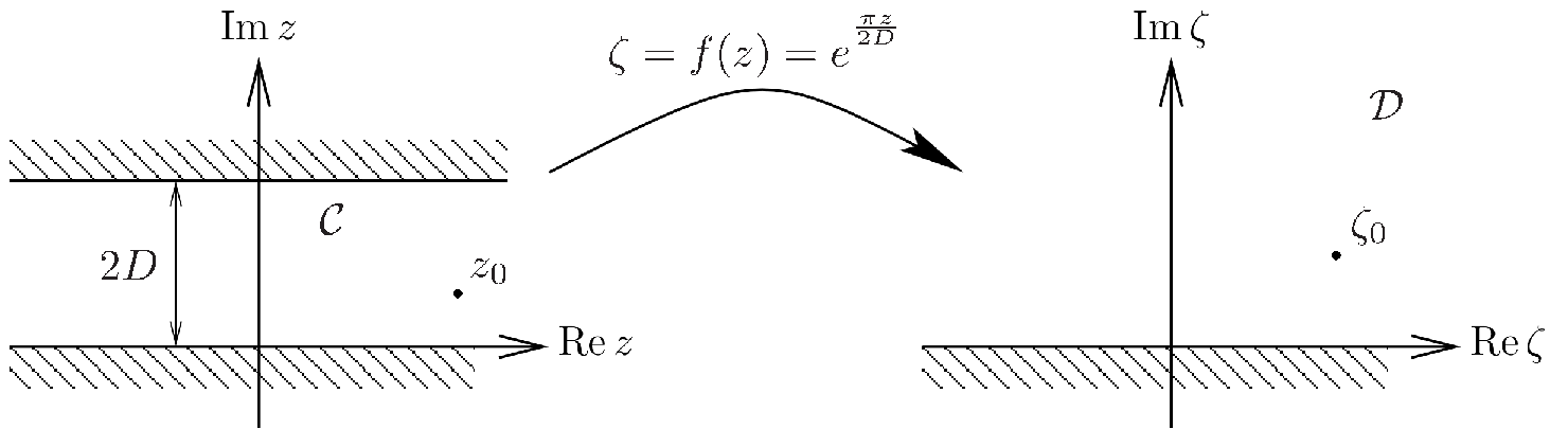
Figure 1: Schematic illustration of the conformal map $\zeta=f(z)=e^{{}^{\frac{\pi z}{2D}}}$ transforming $\mathcal{C}$ onto $\mathcal{D}$ and a vortex placed in $z_{0}$ into a vortex in $\zeta_{0}$, $\zeta_{0}=f(z_{0})$.

The analytical function $f$ transforming conformally the channel $\mathcal{C}=\{z\in\mathbb{C}:0<\Im\text{m}\;z<2D\}$ onto $\mathcal{D}$ is as follows (see Fig. 1 for a schematic illustration)

$$\zeta=f(z)=e^{{}^{\frac{\pi z}{2D}}}\;\;.$$ (8)

The conformal map $f$ transforms $\partial\mathcal{C}$ onto $\partial\mathcal{D}$, with $f(\{z\in\mathbb{C}:\Im\text{m}\;z=0\})=\mathbb{R}^{+}$ and $f(\{z\in\mathbb{C}:\Im\text{m}\;z=2D\})=\mathbb{R}^{-}$. Employing Eq. (6), the determination of the complex potential $\Omega(z)$ is straightforward, namely

$$\Omega(z,z_{0})=-\text{sgn}(z_{0})\frac{i\kappa}{2\pi}\log{\left(\frac{1-e^{{}^{-\frac{\pi}{2D}(z-z_{0})}}}{1-e^{{}^{-\frac{\pi}{2D}(z-z_{0}^{*})}}}\right)}\;\;\;,\;\;\;z_{0}=f^{-1}(\zeta_{0})$$ (9)

leading to the following complex velocity

$$\displaystyle w(z,z_{0}) = -\text{sgn}(z_{0})\frac{i\pi}{4}\frac{\kappa}{2\pi D}\left\{\coth\left[\frac{\pi}{4D}(z-z_{0})\right]-\coth\left[\frac{\pi}{4D}(z-z_{0}^{*})\right]\right\}$$ (10)

$$= \chi(z,z_{0})+\chi(z,z_{0}^{*})\;\;,$$

where $\displaystyle\;\chi(z,z_{0})=-\text{sgn}(z_{0})\frac{i\pi}{4}\frac{\kappa}{2\pi D}\coth\left[\frac{\pi}{4D}(z-z_{0})\right]$ and $\;\text{sgn}(z_{0}^{*})=-\text{sgn}(z_{0})$.
The complex function $\chi(z,z_{0})$ (and, correspondingly, $\chi(z,z_{0}^{*})$) can be physically interpreted as the complex velocity generated by an isolated vortex placed in $z_{0}$ (whose complex potential would be $\Omega(z,z_{0})=-\text{sgn}(z_{0})i\kappa\log(z-z_{0})/(2\pi)$) and its infinite images with respect to the walls of the channel, $\Im\text{m}\;z=0$ and $\Im\text{m}\;z=2D$. The expression (10) for the complex potential $w(z,z_{0})$ can indeed be derived by considering two sets of infinite images of a vortex placed in $z_{0}$ and an anti-vortex in $z_{0}^{*}$ (Greengard, 1990).

If the channel is characterised by the presence of $N$ vortices, the complex velocity $w(z,z_{k_{\{k=1,\dots,N\}}})$ generated by the the set of $N$ vortices is obtained via the superposition principle, i.e.

$$w(z,z_{k_{\{k=1,\dots,N\}}})=\sum_{k=1}^{N}w(z,z_{k})=\sum_{k=1}^{N}\left[\chi(z,z_{k})+\chi(z,z_{k}^{*})\right]\;\;.$$ (11)

A crucial role in this $N$-vortex problem is played by the equations of motion of a generic $j$-th vortex. In order to derive such equations of motions, we define the position $z_{j}(t):=x_{j}(t)+iy_{j}(t)$ occupied by the vortex at time $t$ in the channel $\mathcal{C}$. Indicating with the superscript ‘ $\dot{}$ ’ derivation with respect to time, we define the quantity $\dot{z}_{j}(t):=\dot{x}_{j}(t)+i\dot{y}_{j}(t)$, where the real and imaginary part correspond to the $x$ and $y$ components of the $j$-th vortex velocity. As vortices are advected by the local fluid velocity, i.e. $\dot{\mathbf{x}_{j}}(t)=\mathbf{v}(\mathbf{x}_{j}(t),t)$, the following relation holds

$$\dot{z}_{j}=w^{*}(z_{j},z_{k_{\{k=1,\dots,N\}}})\;\;,$$ (12)

where we have omitted the time dependence of $z_{j}$ and $z_{k}$ to ease notation and the complex conjugation on the r.h.s. arises from the definition (5) of complex velocity. In order to determine the complex velocity $w(z_{j},z_{k_{\{k=1,\dots,N\}}})$, we employ Eq. (11) subtracting the term corresponding to the vortex placed in $z_{j}$, obtaining the following relation

$$\displaystyle\dot{z}_{j} = w^{*}(z_{j},z_{k_{\{k=1,\dots,N;k\neq j\}}})+\chi^{*}(z_{j},z_{j}^{*})$$ (13)

$$= \sum_{k\neq j}w^{*}(z_{j},z_{k})+\chi^{*}(z_{j},z_{j}^{*})$$

$$= \sum_{k\neq j}\left[\chi^{*}(z_{j},z_{k})+\chi^{*}(z_{j},z_{k}^{*})\right]+\chi^{*}(z_{j},z_{j}^{*})\;\;,$$

which coincides with the equations of motion of the $j$-th vortex. The equations of motion of the whole $N$-vortex problem are hence a set of $2N$ coupled ordinary differential equations.

II.2 Gross-Pitaevskii equation model

The Gross-Pitaevskii model is a well-established theoretical framework for the investigation of the dynamics of BECs at temperatures much smaller than the critical transition temperature. The Gross-Pitaevskii (GP) equation describes the temporal evolution of the complex order parameter $\Psi=\Psi(\mathbf{x},t)$ of the system, and reads as follows,

$$i\hbar\dot{\Psi}=-\frac{\hbar^{2}}{2m}\Delta\Psi+V\Psi+g|\Psi|^{2}\Psi\;\;,$$ (14)

where the dot is the time derivative, $\hbar=h/(2\pi)$ is the reduced Planck’s constant, $m$ is the boson mass, $V=V(\mathbf{x},t)$ is an externally applied potential, and $g=4\pi\hbar^{2}a_{s}/m$ models the two-body contact-like boson interaction, where $a_{s}$ is the s-wave scattering length for the collision of two bosons. The order parameter $\Psi$ can be written in terms of its amplitude and its phase as

$$\Psi=\sqrt{n}e^{i\theta}\;,$$ (15)

where $n=n(\mathbf{x},t)=|\Psi|^{2}$ is the particle number density (number of bosons per unit volume) and $\theta=\theta(\mathbf{x},t)$ is the phase. Without loss of generality, the order parameter $\Psi$ can be written as $\Psi(\mathbf{x},t)=e^{i\mu t/\hbar}\Phi(\mathbf{x},t)$ where $\mu$ is called the chemical potential and $\Phi(\mathbf{x},t)$ obeys

$$i\hbar\dot{\Phi}=-\frac{\hbar^{2}}{2m}\Delta\Phi+V\Phi+g|\Phi|^{2}\Phi-\mu\Phi\;\;.$$ (16)

II.2.1 Quantum vortices

In the context of BECs described by the Gross-Pitaevskii equation, quantum vortices are topological defects of the phase $\theta$ of the order parameter, at which $\Psi=0$ (hence $\theta$ is undefined) and around which $\theta$ wraps by $2q\pi$ with $q\in\mathbb{Z}\setminus\{0\}$. In three dimensions, vortices take the form of one-dimensional curves which may form a vortex tangle, as observed both in BECs (White et al., 2010) and superfluid helium (Vinen, 1957). In two dimensions, vortices coincide with vortex points which have been observed extensively in oblate (pancake-like) BECs (Matthews et al., 1999). For the purpose of the present work, we will restrict our discussion to two dimensional systems.

The velocity field $\mathbf{v}(\mathbf{x},t)$ associated to a BECs whose dynamics is described by the order parameter $\Psi$, is defined from the phase $\theta$ via the relation

$$\mathbf{v}(\mathbf{x},t)=\frac{\hbar}{m}\nabla\theta.$$ (17)

Employing the definition (17) of the velocity and the $2q\pi$ phase wrapping existing around a vortex, it is straightforward to verify that the circulation $\Gamma$ of the velocity field on any closed curve $\gamma$ enclosing a vortex point is quantised in terms of the quantum of circulation $\kappa=h/m$, i.e.

$$\Gamma=\oint_{\gamma}\!\!\mathbf{v}\cdot\mathbf{dl}=q\kappa\;\;\;,\;\;\;q\in\mathbb{Z}\setminus\{0\}.$$ (18)

Choosing $\gamma$ to be a circle of radius $r$ and assuming the flow around a vortex to be axisymmetric, the azimuthal component of the flow velocity around a vortex is given by the relation $v_{\phi}=q\kappa/(2\pi r)$, coinciding with the expression for a classical point vortex. Hence, from a velocity point of view, quantum and classical vortices are identical. The important and dynamically significant distinction between classical and quantum vortices is that the latter are characterised by a finite core whose size is of the order of the so-called healing length $\xi=\hbar/\sqrt{mgn}$. As we will very briefly illustrate in the next section, quantum fluids are indeed compressible fluids.

II.2.2 Fluid dynamical equations for a BEC

The Gross-Pitaevskii equation (14) may be rewritten via the Madelung transformation consisting in expressing $\Psi$ in polar form (15) and separating the real and imaginary parts of (14). This procedure leads to the following equations

$$\dot{n}+\nabla\cdot\left(n\mathbf{v}\right)=0,$$ (19)

$$mn\left[\dot{\mathbf{v}}+\left(\mathbf{v}\cdot\nabla\right)\mathbf{v}\right]=-\nabla\left(p+p^{\prime}\right)-n\nabla V,$$ (20)

where $p$ and $p^{\prime}$ are respectively pressure and quantum pressure

$$p=\frac{gn^{2}}{2},$$ (21)

$$p^{\prime}=-\frac{\hbar^{2}}{4m}n\Delta\left(\ln{(n)}\right).$$ (22)

Equation (19) coincides formally with the continuity equation of a classical fluid, while equation (20), exception made for the presence of the quantum pressure $p^{\prime}$, is formally identical to the momentum balance equation for a barotropic, compressible classical Euler (ideal) fluid. At length scales $\ell$ much larger than the healing length $\xi$ (which is the typical length scale for density variations, associated e.g. to the presence of vortices or boundaries) $p^{\prime}/p\ll 1$, implying that in this limit the BEC can indeed be considered as a barotropic, compressible classical inviscid fluid. Hence, at length scales $\ell\gg\xi$, the dynamics of quantum and classical point vortices only differ on the basis of compressible phenomena which may arise in BECs. In the other limit of $\ell\sim\xi$, the physics may be significantly different. For instance, if the relative distance between quantum vortices of opposite sign is of the order of $\xi$, the quantum pressure term would trigger the annihilation of the vortex pair, while in the classical point vortex model no loss of circulation is included in the model. Moreover, the behaviour of a co-rotating pair of quantum vortices of same sign also shows dissimilarities with respect to the classical case, in particular for the finite value of the rotation frequency $\omega_{\tau}$ as the distance $\ell$ tends to zero (in the classical model, the frequency diverges, $\omega_{\tau}\sim 1/\ell^{2}$).

III Results

III.1 Classical fluids

To make progress in understanding the impact of boundaries on the leapfrogging behaviour of classical point vortices in a two-dimensional channel, we consider the motion of four vortices, half with positive circulation $\kappa$, half with negative $-\kappa$. In Fig. 2 we show this initial condition. If we interpret our two-dimensional configuration as a model of a three-dimensional configuration of vortex rings, point vortices of same colour in the figure correspond to cross-sections of the same ring. Initially, the four vortices are vertically aligned on the $y$ axis, i.e. $x_{j}(0)=0$ for $j=1,\dots,4$ and the vortex-anti vortex pairs are symmetrically positioned with respect to the channel mid axis $y=D$, namely $y_{j}(0)=D\pm R$ for the first pair $j=(1,2)$ and $y_{j}(0)=D\pm r$ for the second pair $j=(3,4)$, with the conditions $R/D<1$ and $r/R<1$.

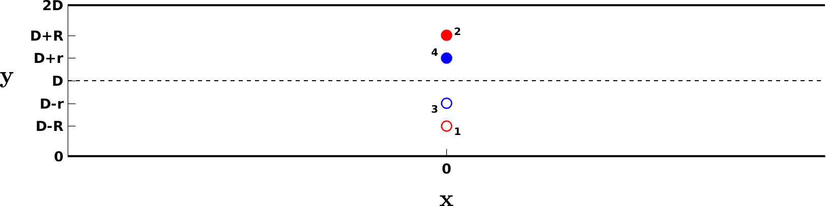
Figure 2: Initial vortex configuration for the classical point vortices numerical simulations: filled (open) circles correspond to vortices with positive (negative) circulation. Numerical labels close to vortices indicate the vortex numeration employed.

In order to characterise the dependence of vortex trajectories on the two non-dimensional parameters $r/R$ and $R/D$ which determine the flow, we numerically integrate the equations of motion (13) for the four vortices, $j=1,\dots,4$, varying $r/R$ and $R/D$. In particular, we choose $r/R=n/10$ and $R/D=m/10$, with $m,n=1,\dots,9$. The time-advancement scheme employed in the numerical simulations is a second-order Adams-Bashforth method with a time step $\Delta t=T/1000$ where $T=2\pi^{2}\delta^{2}/\kappa$ is the rotation period of a pair of vortices of the same polarity placed at distance $\delta$. In our numerical simulations $\delta$ is set to $10^{-3}D$.

For classical unbounded fluids, since the study performed by Love over a century ago (Love, 1894), it is well known that vortices undergo leapfrogging motion only if $r/R$ is larger than a critical value $\alpha_{c}=3-2\sqrt{2}\approx 0.172$. If $r/R<\alpha_{c}$, leapfrogging does not occur: the smaller, faster pair moves “too fast” for the larger ring to influence its dynamics in a significant way, and the vortices separate. More recently, Acheson (Acheson, 2000) extended numerically the study performed by Love and established that leapfrogging motion is unstable when $\alpha_{c}<r/R<\alpha_{c}^{\prime}$, with $\alpha_{c}^{\prime}=0.382$.

In our two-dimensional channel, the confinement of the flow leads to a richer dynamics than in an unbounded domain. In addition to distinction between leapfrogging and non-leapfrogging, which is already known, we also observe backward leapfrogging and periodic orbits. The phase diagram of the system resulting from the numerical simulations is illustrated in Fig. 3.

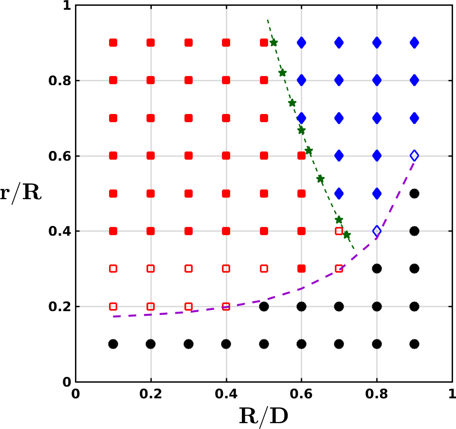
Figure 3: Phase diagram of the classical motion of two vortex-anti vortex pairs in a two-dimensional plane channel. All symbols refer to performed numerical simulations. Black circles indicate no leapfrogging motion; red filled (open) squares stand for stable (unstable) forward, standard leapfrogging; blue filled (open) diamonds correspond to stable (unstable) backward leapfrogging; green stars stand for periodic orbits. The dashed green line indicates the analytical solution for periodic orbits (see section III.1.1 and Appendix). The dashed violet curve is the numerically computed $\alpha_{c}$ dependence on $(R/D)$.

For values of $R/D\leq 1/2$, the dynamics is very similar to what is observed in an unbounded fluid, the role of the boundaries being only marginal. For a given value of $R/D\leq 1/2$, in fact, as we increase $r/R$, we first observe non leapfrogging motion (in black in Fig. 3), defined as the dynamics characterised by $\dot{y}_{j}(t)=0$ for all $j$ at late times; then we notice unstable leapfrogging motion (open red squares), and finally stable leapfrogging (filled red squares). These dynamical regimes therefore coincide with the scenario outlined by Acheson (Acheson, 2000), the only significant and important difference being the dependence of $\alpha_{c}$ on $R/D$: for small values of $R/D$, $\alpha_{c}$ is very close to the constant value $0.172$ for vortex leapfrogging in unbounded fluids (e.g. for $R/D=0.1$, $\alpha_{c}=0.173$), increasing for increasing values of $R/D$ (e.g. $\alpha_{c}=0.216$ for $R/D=0.5$). This dependence of $\alpha_{c}$ on $R/D$ stems from the interaction of the outer vortices 1 and 2 in Fig. 2) with their corresponding images with respect to the closest channel wall; essentially, the interaction with image vortices is stronger compared to the interaction of the inner pair with the corresponding images. These images, of opposite sign, slow down the outer vortex pair, allowing the inner pair to escape towards infinity for values of $r/R$ which would produce leapfrogging motion in an unbounded fluid; in order to recover leapfrogging, $r/R$ would have to increase. As $R/D$ increases, this effect is amplified as the outer pair is closer to the channel walls.

This increasing monotonous behaviour of $\alpha_{c}$ with respect to $R/D$ extends also for $R/D>1/2$, where the role played by boundaries becomes significant, triggering a much richer dynamics. As $R/D$ is larger than $1/2$, for large values of $r/R$, we observe backward-leapfrogging, indicated by blue diamonds in Fig. 3. This dynamics, again, originates from the interaction of vortices with their images with respect to the closest channel wall. In particular, each vortex, paired to its image of opposite sign, forms a virtual vortex-anti vortex pair on its own. As a consequence, we observe two distinct leapfrogging motions, each involving two virtual vortex-anti vortex pairs. Due to the vortex polarity, the leapfrogging motion induces a net translation in the opposite direction with respect to standard (forward) leapfrogging. In the $(R/D,r/R)$ plane, the forward-leapfrogging to backward-leapfrogging transition occurs via an intermediate regime in which vortices follow periodic orbits, indicated by green stars in Fig. 3. As shown in detail in the next section and in the analytical derivation presented in the Appendix, periodic orbits are observed when $R+r=D$, corresponding to the green dashed line in Fig. 3. For large values of $R/D$ ($R/D\gtrsim 3/4$), the system crosses directly the no-leapfrogging to backward-leapfrogging boundary without passing through a forward-leapfrogging regime. Examples of all the different regimes observed in our system of classical point vortices are shown in Fig. 4. Note that in the three-dimensional coaxial vortex rings analog, vortices of the same colour correspond to cross-sections of the same vortex ring.

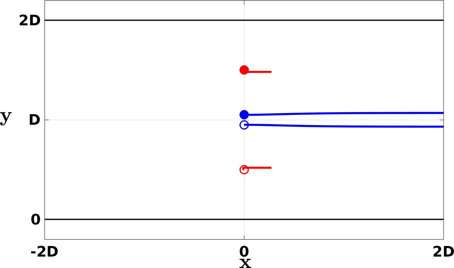
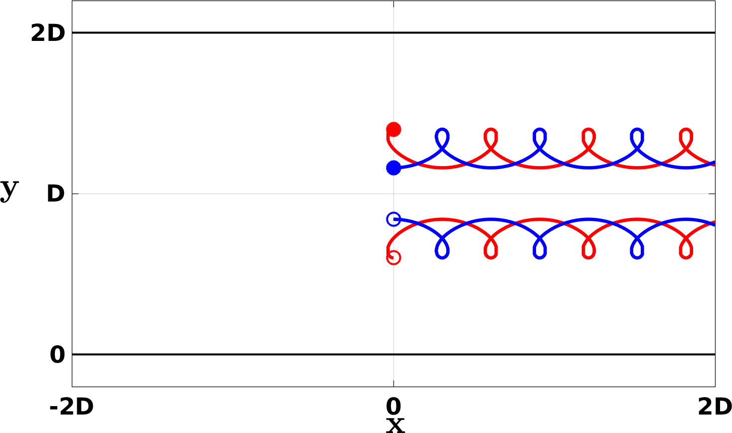
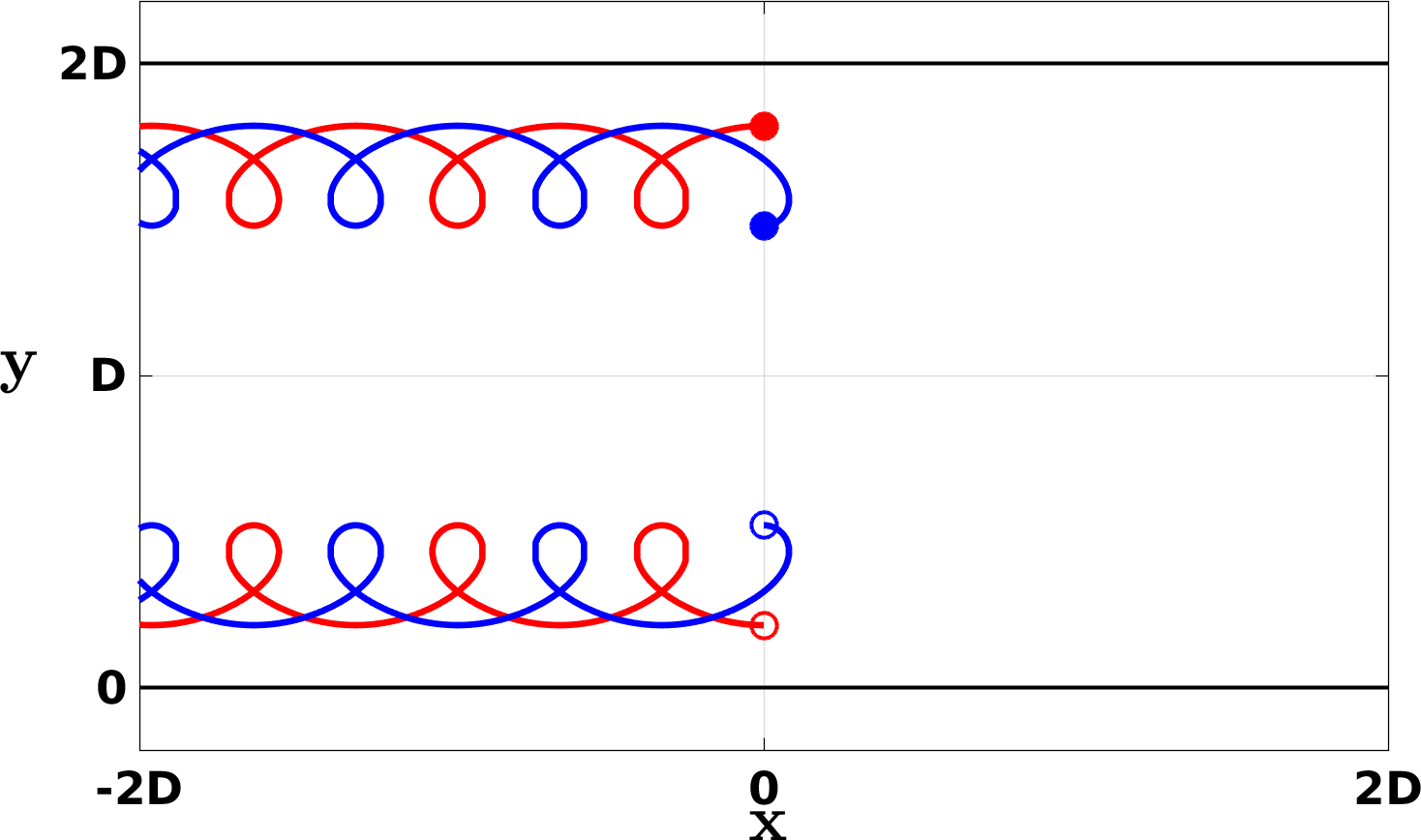
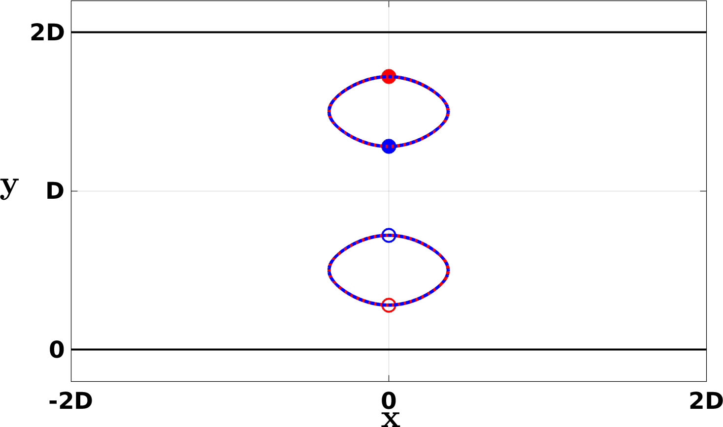
Figure 4: Examples of dynamical regimes and trajectories for classical 4-vortex motion in a two-dimensional channel. Filled (open) symbols indicate positive (negative) vortices. Top Left: $R/D=5/10$, $r/R=1/10$, no-leapfrogging (vortices moving to the right). Top Right: $R/D=4/10$, $r/R=4/10$, forward (standard) leapfrogging (vortices moving to the right). Bottom Left: $R/D=8/10$, $r/R=6/10$, backward-leapfrogging (vortices moving to the left); Bottom Right: $R/D=72/100$, $r/R=39/100$, periodic orbits.

III.1.1 Derivation of periodic orbits

In this section we derive theoretically the existence of periodic orbits in the leapfrogging motion of four vortices in a channel using the classical point-vortex model. We show that under suitable conditions, namely when $R+r=D$, each pair of same signed vortices moves around a fixed point. Some analytic details are discussed in the Appendix.

With reference to Fig. 2, we consider the pair of vortices $P_{1}=(x_{0}(t),D-R(t))$, with negative circulation $-\kappa$, and $P_{2}=(x_{0}(t),D+R(t))$, with positive circulation $\kappa$, and the pair of vortices $P_{3}=(x_{1}(t),D-r(t))$, with negative circulation $-\kappa$, and $P_{4}=(x_{1}(t),D+r(t))$, with positive circulation $\kappa$, where $t$ is time. In the complex domain, omitting the time dependence to ease notation, these vortices are located in $z_{1}=x_{0}+i(D-R)$ for $P_{1}$, $z_{2}=x_{0}+i(D+R)$ for $P_{2}$, $z_{3}=x_{1}+i(D-r)$ for $P_{3}$ and $z_{4}=x_{1}+i(D+r)$ for $P_{4}$, and they generate the following complex velocity in the point $z$, as given by Eq. (11),

$$w(z)=w(z,z_{1})+w(z,z_{2})+w(z,z_{3})+w(z,z_{4})\;\;.$$ (23)

We now consider the midpoint $M$ between the vortex points $P_{1}$ and $P_{3}$, namely $\displaystyle z_{M}(t)~{}=~{}\frac{x_{0}(t)+x_{1}(t)}{2}+i\left(D-\frac{r(t)+R(t)}{2}\right)$ and the complex velocity generated by vortices in $z_{M}$ which we indicate with $w(z_{M})$

$$w(z_{M})=\frac{\frac{i\kappa}{2D}\left(-1+e^{\frac{2i\pi(r+R)}{D}}\right)e^{\frac{\pi(\text{x}_{0}+\text{x}_{1})}{2D}}}{\left(e^{\frac{\pi(4ir+4iR+\text{x}_{0}+\text{x}_{1})}{2D}}-e^{\frac{\pi(2\text{x}_{0}+i(r+3R))}{2D}}-e^{\frac{\pi(2\text{x}_{1}+i(3r+R))}{2D}}+e^{\frac{\pi(\text{x}_{0}+\text{x}_{1})}{2D}}\right)}\;\;.$$ (24)

If we look for the conditions such that the velocity $w(z_{M})$ of the midpoint $M$ is zero, we have

$$w(z_{M})=0\quad\Longleftrightarrow\quad e^{\frac{2i\pi(r+R)}{D}}-1=0\quad\Longleftrightarrow\quad\frac{2\pi(r+R)}{D}=2k\pi\;,\quad k\in\mathbb{Z}\;\;.$$ (25)

Note that the same result Eq. (25) is found for the midpoint $N$ between the two vortex points $P_{2}$ and $P_{4}$.

Since $r$, $R$, and $D$ are positive real parameters, the only admissible values of $k$ in (25) are $k\in\mathbb{Z}^{+}$. Moreover, we know that $r<R<D$, leading to $r+R<2D$, which implies that the only admissible value for $k$ is $k=1$, i.e.

$$r(t)+R(t)=D\;\;.$$ (26)

This is the most interesting result: it states that when the four vortices satisfy the condition (26) then the midpoints $M$ and $N$ are at rest: the two pairs of vortices $(P_{1},\,P_{3})$ and $(P_{2},\,P_{4})$ move hence symmetrically with respect to their correspondent midpoints, i.e. $\dot{x}_{0}(t)=-\dot{x}_{1}(t)$ and $\dot{R}(t)=-\dot{r}(t)$. The last equality is fundamental as it expresses that if condition (26) is satisfied at a given $t=t_{0}$, it will be satisfied for every $t>t_{0}$. Thus, if the initial condition is prepared such that $x_{0}(0)=x_{1}(0)=0$ and $r(0)+R(0)=D$, vortices will always move symmetrically with respect to their midpoints $\displaystyle z_{M}=i\frac{D}{2}$ and $\displaystyle z_{N}=i\frac{3D}{2}$.

The last step to demonstrate the existence of periodic orbits is to prove that the trajectories of the vortex points are closed curves rotating around the two midpoints $M$ and $N$ as, in principle more general trajectories with the restriction $\dot{R}(t)=-\dot{r}(t)$ (for instance, $\dot{R}(t)=\dot{r}(t)=0$) could be possible, not leading to periodic orbits. We tackle this issue in the Appendix, to ease the readability of the manuscript.

III.2 Quantum fluids

The next step is to numerically probe the dynamical regimes of two quantum vortex-antivortex pairs interacting in a two-dimensional channel. We shall compare the results with the corresponding classical results outlined in the previous Section (III.1).

We consider a two-dimensional BEC in a channel geometry, imprinting quantum vortices in the positions initially occupied by classical vortices. Note that, in addition to the parameters $R$, $r$ and $D$ already present in the classical point vortex formulation, in the Gross-Pitaevskii formulation of the problem we have an extra length scale - the healing length $\xi$ - which plays a fundamental role in the dynamics. To assess the relevance of this extra length scale, we present numerical simulations of leapfrogging quantum vortices employing two distinct values of the channel half-width $D$: $D_{1}=40\xi$ and $D_{2}=20\xi$. In order to model the channel confinement, we use the following potential $V$:

$$V=V(y)=\begin{cases}0&\text{if }0<y<2D\\[8.53581pt] 10\mu&\text{if }\;y\leq 0\;\;\text{or }\;y\geq 2D,\end{cases}$$ (27)

corresponding to a channel of half-width $D$, where the density $|\Phi|^{2}$ is constant everywhere with the exception of thin layer whose width is of the order of the healing length at the channel boundaries $y=0$ and $y=2D$.

The trajectories of the quantum vortices are calculated as a function of time by numerically solving the equation of motion of the order parameter $\Phi$, the dimensionless Gross-Pitaevskii equation

$$i\dot{\Phi}=-\frac{1}{2}\Delta\Phi+\frac{V}{\mu}\Phi+|\Phi|^{2}\Phi-\Phi\;\;.$$ (28)

Equation (28) is obtained from Eq. (16) after introducing characteristic units of length, time and energy: $\xi=\hbar/\sqrt{m\mu}$ (the healing length), $\tau=\xi/c\;$ (where $c=\sqrt{\mu/m}$ is the speed of sound), and $\mu$ (the chemical potential) respectively, and normalising the order parameter with respect to the unperturbed homogeneous solution $\Phi_{0}=\sqrt{\mu/g}$ of Eq. (16). In these units the healing length and the bulk density in the channel are unity.

The numerical integration of Eq. (28) is performed employing a fourth-order Runge-Kutta time advancement scheme and second-order finite differences to approximate spatial derivative operators. Time step $\Delta t/\tau$ is set to $1.5\times 10^{-2}$ and spatial discretization $\Delta x/\xi=\Delta y/\xi$ is chosen to be equal to $0.25$. In the set of simulations where $D=D_{1}=40\xi$, the numbers of grid-points in the $x$ and $y$ directions are $N_{x}=6400$ and $N_{y}=400$ respectively, leading to the computational box $-800\xi\leq x\leq 800\xi$ and $-10\xi\leq y\leq 90\xi$. On the other hand, when $D=D_{2}=20\xi$, $N_{x}=3200$ and $N_{y}=240$ respectively, leading to the computational box $-400\xi\leq x\leq 400\xi$ and $-10\xi\leq y\leq 50\xi$.

The initial imprinting of vortices is made by enforcing a uniform $2\pi$ phase wrapping around the positions employed as initial condition for the classical point vortex simulations and letting the system relax in imaginary time before starting the integration of Eq. (28) for $t\in\mathbb{R}$. In Fig. 5 we report the density $|\Phi|^{2}(x,y)$ (left) and the phase $\theta(x,y)$ (right) of the initial condition employed for $R/D=0.6$ and $r/R=0.3$ and $D=D_{1}=40\xi$. It can be easily observed that the density $|\Phi|^{2}$ rapidly drops to zero at the vortex positions and outside the channel. Correspondingly, the four $2\pi$ phase wrappings can be distinguished in Fig. 5 (right).

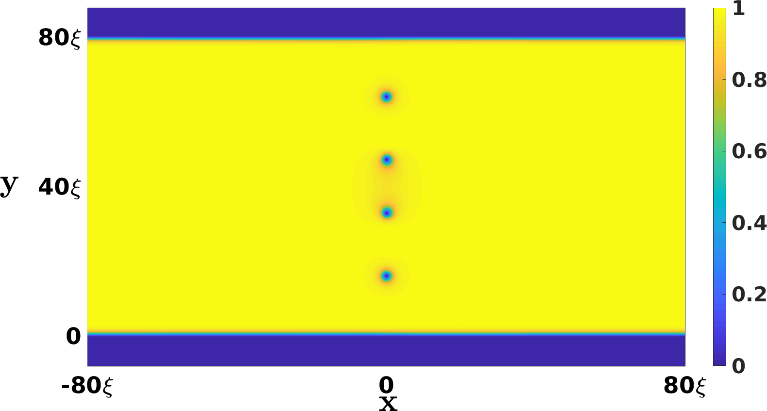
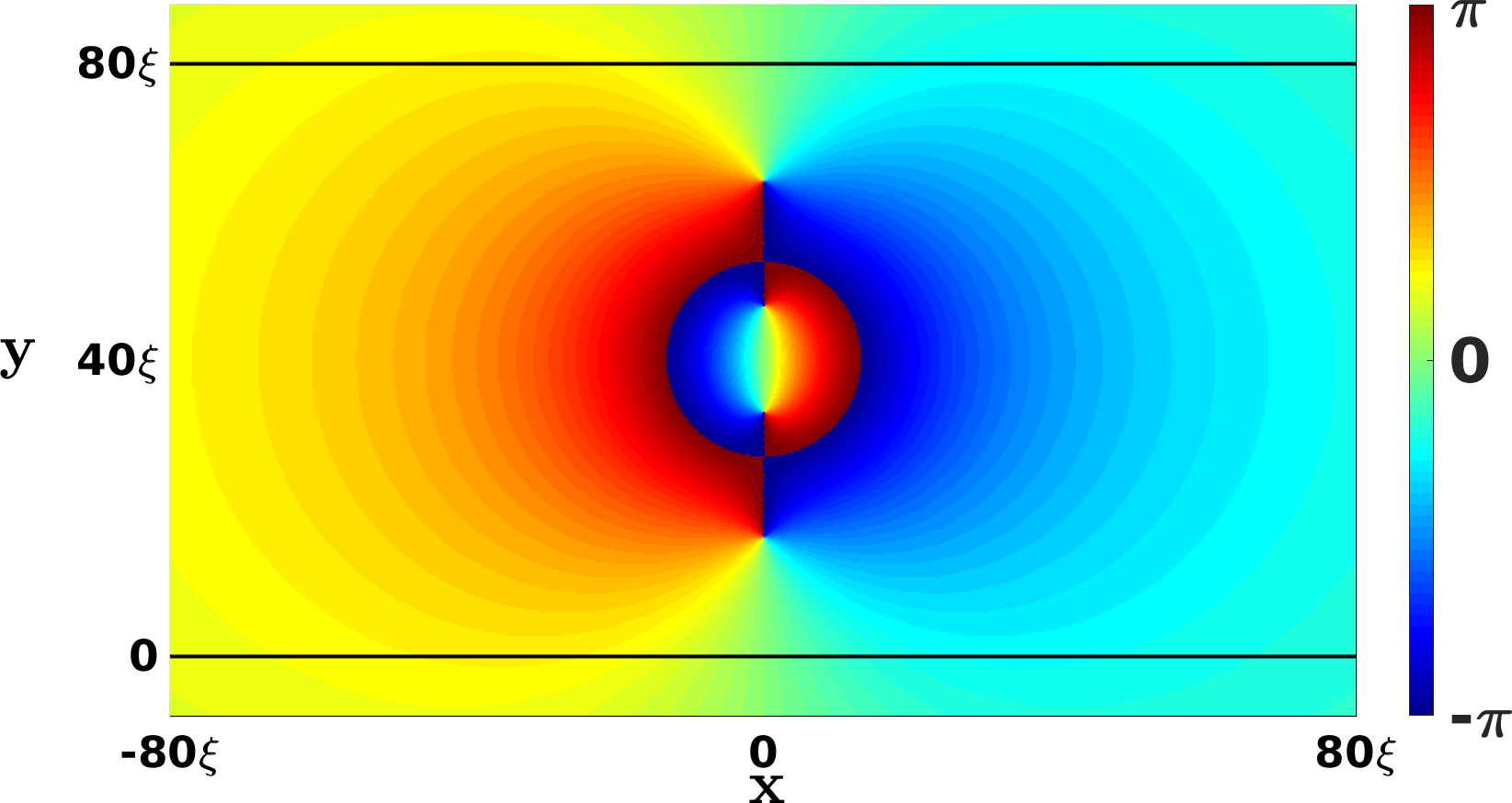
Figure 5: Initial condition for numerical simulation of leapfrogging of quantum vortices in a two dimensional channel for $R/D=0.6$ and $r/R=0.3$ and $D=D_{1}=40\xi$. (Left) the density of the BEC $|\Phi(x,y)|^{2}$ (presented as a ratio of the bulk density $|\Phi_{0}|^{2}$) is displayed: it is unity (yellow) in the bulk of the channel and vanishes (blue) in the vortex cores and at the channel’s boundaries; (right) the phase $\theta(x,y)$ of the BEC is illustrated in the range $[-\pi,\pi)$.

To verify the existence in a BEC of all distinct regimes observed in the classical point vortex model (Section III.1), we perform numerical simulations of quantum vortex leapfrogging along the vertical line $R/D=0.6$ of the phase-diagram reported in Fig. 3; we have chosen this value of $R/D$ because along this line, as $r/R$ varies from $1/10$ to $9/10$, all regimes which we have identified using the classical point vortex model are present.

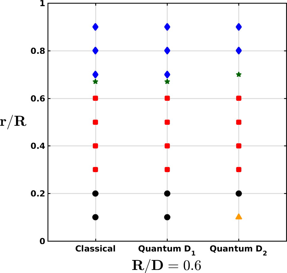
Figure 6: Cuts in the dynamical regimes phase diagram corresponding to $R/D=0.6$ for the classical point vortex model (left), the Gross-Pitaevskii model with $D=D_{1}=40\xi$ (middle) and $D=D_{2}=20\xi$ (right). Symbols as in Fig 3 except for the newly introduced up-pointing orange triangle corresponding to the annihilation of the inner vortex-anti vortex pair.

The results are schematically outlined in Fig. 6, where classical vortex dynamics (left) is compared to quantum vortex dynamics at $D=D_{1}=40\xi$ (middle) and $D=D_{2}=20\xi$ (right). When $D=D_{1}$, the boundaries of the phase diagram at $R/D=0.6$ are at the same values of $r/R$ in the classical and in the quantum case. When $D=D_{2}$ we observe two differences: first, periodic motion now occurs at $(R/D,r/R)=(0.6\,,\,0.7)$ instead of $(R/D,r/R)=(0.6\,,\,0.67)$; second, at $(R/D,r/R)=(0.6\,,\,0.1)$ the internal vortex-anti vortex pair annihilates as their initial distance is only $2.4\xi$. These differences at the smaller value of channel size are expected, as the healing length scale starts playing a role: only if $D/\xi$ is sufficiently large we can expect classical and quantum dynamics to be the same.

The exact matching of the observed dynamical regimes when comparing classical and quantum leapfrogging in a two-dimensional channel if $D\geq 40\xi$ is confirmed in Fig. 7, which shows the trajectories of quantum vortices for $(R/D\,,r/R)$ pairs selected as for the classical trajectories illustrated in Fig. 4.

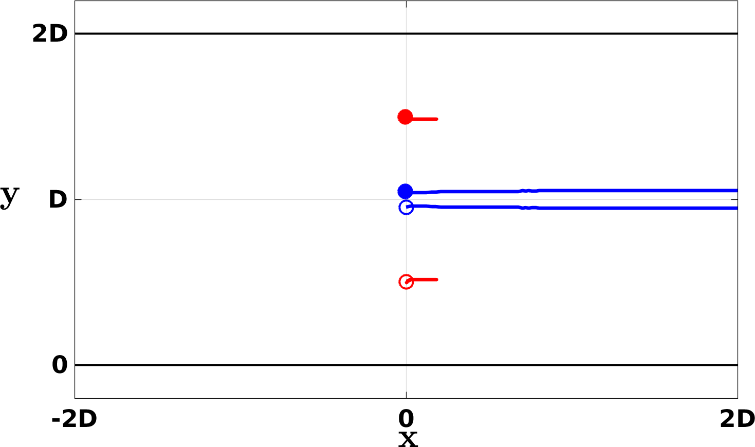
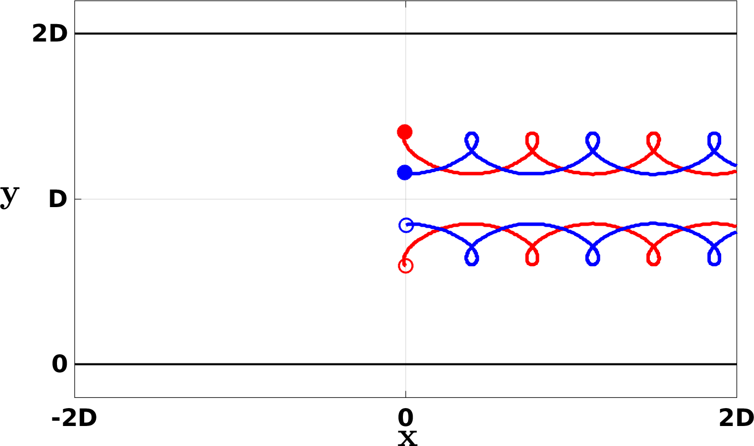
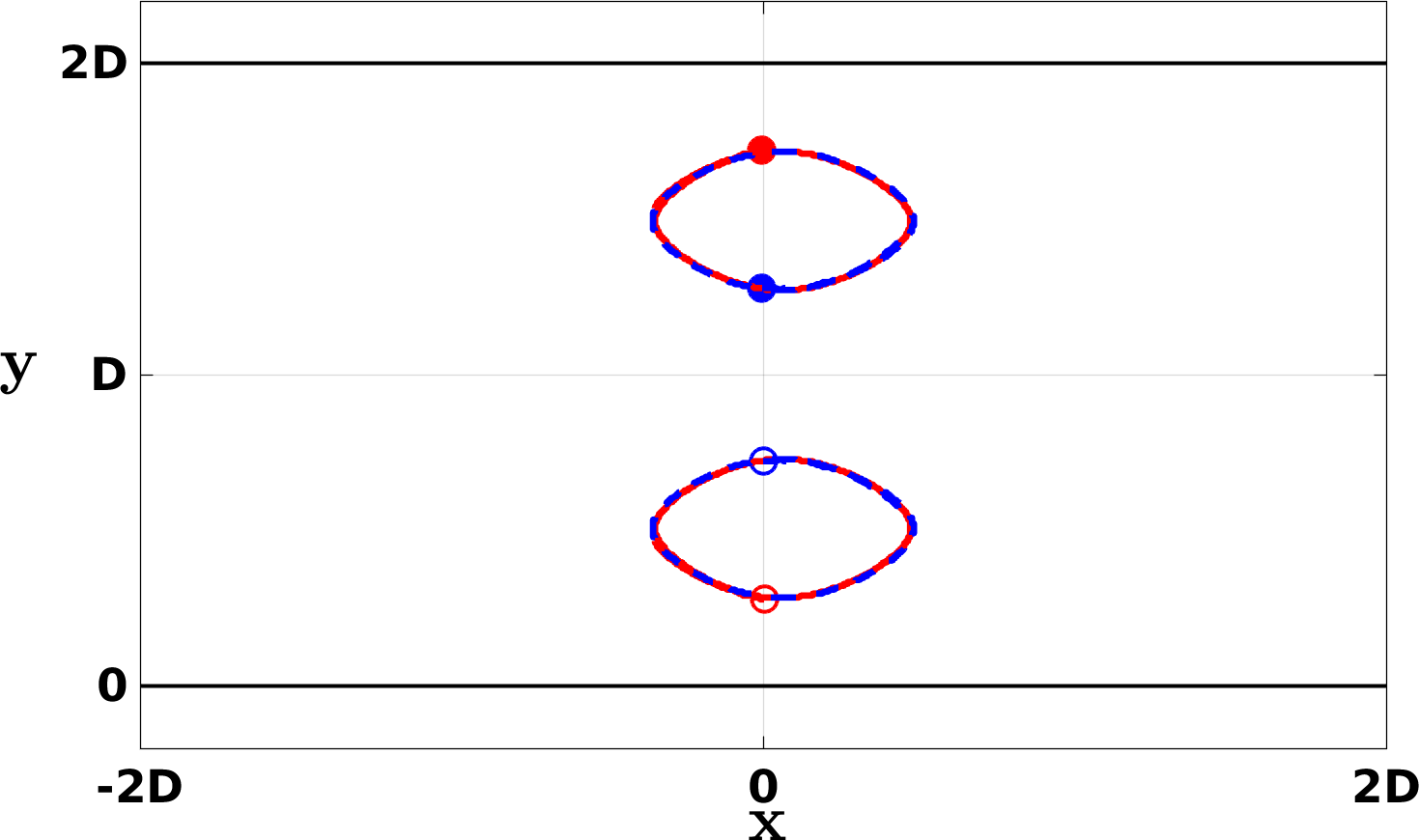
Figure 7: Dynamical regimes observed in a quantum 4-vortex configuration in a two-dimensional channel. Filled (open) symbols indicate positive (negative) vortices. Top Left: $R/D=5/10$, $r/R=1/10$, no leapfrogging motion is observed. Top Right: $R/D=4/10$, $r/R=4/10$, forward (standard) leapfrogging. Bottom Left: $R/D=8/10$, $r/R=6/10$, backward-leapfrogging; Bottom Right: $R/D=72/100$, $r/R=39/100$, periodic orbits.

It is worth noting some minor differences between the quantum vortex trajectories and their classical counterparts reported in Fig. 4. Since the initial condition is not stationary with respect to any frame of reference, when we start integrating in time Eq. (28) for $t\in\mathbb{R}$ there is a sudden emission of sound waves, and as a result the entire vortex configuration is translated towards the positive $x$ direction. The effect (which has been reported in the literature (Frisch et al., 1992)), is visible in the top right, bottom left and bottom right panels of Fig. 7 when compared Fig. 4. In particular, this horizontal shift affects the periodic orbits reported in Fig. 7 (bottom right) whose center is slightly shifted towards positive $x$ values. In addition, the number of periods observed in the $x$ range $[-2D,\,2D]$ is different from the classical counterpart, possibly due to the compressible nature of a quantum Bose gas, in which incompressible kinetic energy may be transformed into compressible kinetic energy (sound) when vortices change their velocities (accelerate), as shown by Parker et al. (2004), exactly as the accelerated motion of charged particles emit electro-magnetic radiation. The role played by this effective dissipation of kinetic energy into sound will be assessed in a future study.

IV Conclusions

In conclusion, we have demonstrated that, in the confined space of a two dimensional channel, the classical problem of vortex leapfrogging acquires new aspects. Using the point vortex model we have found that, besides the known regimes of standard leapfrogging and absence of leapfrogging, there are two new regimes: backward leapfrogging and periodic motion. Using the Gross-Pitaevskii equation to model an atomic Bose-Einstein condensate (a compressible quantum fluid) confined within a channel, we have verified that all four regime also exist for quantum vortices. In large channels, the boundaries between these regimes are the same for classical and quantum vortices. Some differences appear if the channel size is reduced, and the finite-size nature of the quantum vortex core starts playing a role, or if the vortices are very close and sound radiation becomes important. The determination of a richer dynamics for the leapfrogging of vortices occuring in confined geometries will be particularly important for the interpretation and planning of ongoing and future experiments with atomic Bose-Einstein Condensates, where the dynamical regimes reported in the present work can be potentially observed.

Future work will address the problem in three dimensions, paying attention to the excitation of Kelvin waves along the vortex rings and the departure from axisymmetry.

V Acknowledgements

LG, NGP and CFB acknowledge the support of the Engineering and Physical Sciences Research Council (grant No. EP/R005192/1). M.S. acknowledges the support of MIUR-Italy through the project PRIN “Multiscale phenomena in Continuum Mechanics: singular limits, off-equilibrium and transitions” (grant No. PRIN2017 2017YBKNCE).

Declaration of Interests. The authors report no conflict of interest.

Appendix A Derivation of periodic orbits

In order to show the existence of periodic orbits, we have to prove that if condition (26) is satisfied, the trajectories of the vortex points are closed curves with vortices rotating around the two midpoints $M$ and $N$ defined in section III.1.1.

For the sake of simplicity, and with reference to section III.1.1, we prove the closedness of the trajectory only for the vortex point $P_{1}$, as the proof for the other vortex points is an iterative procedure. We consider equation (12) for the vortex point $z_{1}$ with the complex velocity given by the expression (23) evaluated on the vortex point $z_{1}$. Since the middle point $z_{M}$ is at rest for $r+R=D$, we rewrite the dynamic equation of $z_{1}$, namely $\dot{z_{1}}=w^{*}(z_{1})$, in the polar coordinate system $(\rho,\,\theta)$ centered on $z_{M}$. The middle point $z_{M}$, under the condition $r+R=D$, becomes $\displaystyle z_{M}~{}=~{}\frac{x_{0}+x_{1}}{2}+i\frac{D}{2}$, which requires the condition $\displaystyle\rho<\frac{D}{2}$ to ensure that vortices $P_{1}$ and $P_{3}$ are in $\{z\in\mathbb{C}:0<\Im\text{m}\;z<D\}$.

Thus, in the new reference system the vortex points correspond to

$$\begin{array}[]{ll}z_{1}=z_{M}-\rho\cos(\theta)-i\rho\sin(\theta),\\ z_{2}=z_{M}+iD-\rho\cos(\theta)+i\rho\sin(\theta),\\ z_{3}=z_{M}+\rho\cos(\theta)+i\rho\sin(\theta),\\ z_{4}=z_{M}+iD+\rho\cos(\theta)-i\rho\sin(\theta),\\ \end{array}$$ (29)

where $z_{M}$ is now the origin of the new frame of reference, which can be set $z_{M}=0+0i$. Note that the condition (26) is automatically satisfied by construction; indeed, $\displaystyle\frac{z_{2}-z_{1}}{2}~{}=~{}i~{}\left(\frac{D}{2}+\rho\sin(\theta)\right)$ and $\displaystyle\frac{z_{4}-z_{3}}{2}~{}=~{}i~{}\left(\frac{D}{2}-\rho\sin(\theta)\right)$, implying $\displaystyle R~{}\equiv~{}\frac{D}{2}+\rho\sin(\theta)$ and $\displaystyle r~{}\equiv~{}\frac{D}{2}-\rho\sin(\theta)$ and, hence, condition (26). We now substitute the coordinates (29) into the equation

$$\dot{z}_{1}=w^{*}(z_{1},z_{k_{\{k=1,\dots,4\}}}),$$ (30)

according to (12), and change the vectorial basis from $(\hat{\mathbf{x}},\,\hat{\mathbf{y}})$ to $(\hat{\mathbf{u}}_{\rho},\,\hat{\mathbf{u}}_{\theta})$ by means of the following rotation:

$$\hat{\mathbf{u}}_{\rho}=\cos(\theta)\hat{\mathbf{x}}+\sin(\theta)\hat{\mathbf{y}},\qquad\hat{\mathbf{u}}_{\theta}=-\sin(\theta)\hat{\mathbf{x}}+\cos(\theta)\hat{\mathbf{y}}.$$

By writing $\dot{z_{1}}=-\dot{\rho}\hat{\mathbf{u}}_{\rho}-\rho\dot{\theta}\hat{\mathbf{u}}_{\theta}$, we then find the following equations for $\dot{\rho}$ and $\dot{\theta}$:

$$\dot{\rho}=f_{1}(\rho,\,\theta)= \frac{k}{4D}\text{csch}\left(\frac{\pi e^{-i\theta}\rho}{D}\right)\text{csch}\left(\frac{\pi e^{i\theta}\rho}{D}\right)\left[\cos(\theta)\tan\left(\frac{\pi\rho\sin(\theta)}{D}\right)\cosh^{2}\left(\frac{\pi\rho\cos(\theta)}{D}\right)\right.$$ (31)

$$\left.-\sin(\theta)\cos^{2}\left(\frac{\pi\rho\sin(\theta)}{D}\right)\tanh\left(\frac{\pi\rho\cos(\theta)}{D}\right)\right]$$

$$\dot{\theta}=f_{2}(\rho,\,\theta)= -\frac{k}{4D\rho}\text{csch}\left(\frac{\pi e^{-i\theta}\rho}{D}\right)\text{csch}\left(\frac{\pi e^{i\theta}\rho}{D}\right)\left[\cos(\theta)\cos^{2}\left(\frac{\pi\rho\sin(\theta)}{D}\right)\tanh\left(\frac{\pi\rho\cos(\theta)}{D}\right)+\right.$$ (32)

$$\left.+\sin(\theta)\tan\left(\frac{\pi\rho\sin(\theta)}{D}\right)\cosh^{2}\left(\frac{\pi\rho\cos(\theta)}{D}\right)\right]$$

From equations (31) and (32), we finally derive the equation for $\rho^{\prime}=\text{d}\rho/\text{d}\theta$ as follows:

$$\rho^{\prime}=\frac{\dot{\rho}}{\dot{\theta}}=\frac{\rho\sin(\theta)\cos^{2}\left(\frac{\pi\rho\sin(\theta)}{D}\right)\tanh\left(\frac{\pi\rho\cos(\theta)}{D}\right)-\rho\cos(\theta)\tan\left(\frac{\pi\rho\sin(\theta)}{D}\right)\cosh^{2}\left(\frac{\pi\rho\cos(\theta)}{D}\right)}{\cos(\theta)\cos^{2}\left(\frac{\pi\rho\sin(\theta)}{D}\right)\tanh\left(\frac{\pi\rho\cos(\theta)}{D}\right)+\sin(\theta)\tan\left(\frac{\pi\rho\sin(\theta)}{D}\right)\cosh^{2}\left(\frac{\pi\rho\cos(\theta)}{D}\right)}\,,\\$$ (33)

which is well-defined in $\mathcal{A}=\{(\rho,\theta)\in\mathbb{R}^{+}\times\mathbb{R}:0<\rho<D/2\,\}$ because: a) all the elementary functions are well-defined (included the function $\tan(...)$ through the condition $0<\rho<D/2$); b) the denominator is positive (in the first term $\cos(\theta)\cdot\tanh\left(\frac{\pi\rho\cos(\theta)}{D}\right)\geq 0$ and in the second term $\sin(\theta)\cdot\tan\left(\frac{\pi\rho\sin(\theta)}{D}\right)\geq 0$) and never zero (both terms are never zero in $\mathcal{A}$).

In order to prove that the trajectory of vortex $P_{1}$ is a closed curve, we need to show that the function $\rho(\theta)$ is a continuos and periodic function. However, the integration of equation (33) is a hard task to achieve. Therefore, we choose to prove that $\rho(\theta)$ is a continuos and periodic function without finding the exact integral of (33). In order to achieve this goal, we first need to recall a result from mathematical analysis, which states:

Theorem 1

   Given a continuos and periodic function ${\displaystyle f:\mathbb{R}\to\mathbb{R}}$ with period $T$ such that $\displaystyle\int_{0}^{T}f(x)\,{\rm d}x=0$, then the primitive function of $f(x)$ is periodic with period $T$.

Having recalled Theorem 1, we now need to prove the following theorem:

Theorem 2

   The primitive function $\rho(\theta)$ of $\rho^{\prime}(\theta)$ (as defined in (33)) is $C^{1}(\mathbb{R})$ and periodic with period at least $2\pi$.

The proof consists in three steps:

• $\rho(\theta)$ is $C^{1}(\mathbb{R})$ function;
  

• $\rho^{\prime}(\theta)$ is a periodic function, at least of period $T=2\pi$;
  

• $\displaystyle\int_{0}^{2\pi}\rho^{\prime}(\theta)\;{\rm d}\theta=0$.

Below the proof of each step:

• As stated in the previous sections, the complex velocity $w(z)$ is an analytic function, and hence the curve describing the trajectory of the vortex point $P_{1}$. This implies that the function $\rho(\theta)$ is $C^{1}(\mathbb{R})$. Moreover, we can assert that the denominator of $\rho^{\prime}(\theta)$ is $\neq 0$, or, better, it is easy to show that it is always positive for $(\rho,\theta)\,\in\mathcal{A}$. Indeed, the two terms in the denominator in (33) are always positive (both for $\sin\theta$ and $\cos\theta$ positive, negative or null).
  

• $\rho^{\prime}(\theta)$ is a periodic function: in fact it follows directly from (33) that

  $$\rho^{\prime}(\theta+2\pi)=\rho^{\prime}(\theta).$$ (34)

  
  

• A sufficient condition to prove the last step is that the function $\displaystyle\rho^{\prime}(\theta)$ is an odd function in $\mathbb{R}$. The proof follows directly from (33) after substituting $\theta$ by $-\theta$ obtaining:

  $$\rho^{\prime}(-\theta)=-\rho^{\prime}(\theta)$$ (35)

Finally, we apply Theorem 1 to our function $\rho^{\prime}(\theta)$ and the theorem is proved. Theorem 2 leads hence to the conclusion that $\rho(\theta+2\pi)=\rho$ and thus that the trajectory of vortex point $P_{1}$ is a closed curve.

References

- Acheson (2000) Acheson, D. J. 2000 Instability of vortex leapfrogging. Eur. J. Phys. 21, 269–273.
- Aioi et al. (2011) Aioi, T., Kadokura, T., Kishimoto, T., & Saito, H. 2011 Controlled generation and manipulation of vortex dipoles in a Bose-Einstein condensate. Phys. Rev. X 1, 021003.
- Barenghi el al. (2005) Barenghi, C. F., Parker, N. G., Proukakis, N. P., & Adams, C. S. 2005 Decay of quantised vorticity by sound emission. J. Low Temp. Phys. 138, 629.
- Barenghi & Parker (2016) Barenghi, C. F., & Parker, N. G. 2016 A Primer on Quantum Fluids, Springer.
- Berloff et al. (2014) Berloff, N. G., Brachet, M., and Proukakis, N. P. 2014 Modeling quantum fluid dynamics at nonzero temperatures. Proc. Natl. Acad. Sci. USA 111, 4675
- Billam et al. (2014) Billam, T.P., Reeves, M.T., Anderson, B.P., & Bradley, A.S. 2014 Phys. Rev. Lett. 112, 145301.
- Blakie et al. (2014) Blakie, P., Bradley, A., Davis, M., Ballagh, R., & Gardiner, C. 2008 Dynamics and statistical mechanics of ultra-cold Bose gases using c-field techniques. Adv. Phys. 57, 363.
- Breczyk et al. (2007) Brewczyk, M., Gajda, M., & Rzazewski, K. 2007 Classical fields approximation for bosons at nonzero temperatures. J. Phys. B 40, R1.
- Bisset et al. (2015) Bisset, R. N., Wang, W., Ticknor, C., Carretero-Gonzales, R., Frantzeskakis, D. J., Collins, L. A., & Kevrekidis, P. G. 2015 Bifurcation and stability of single and multiple vortex rings in three-dimensional Bose-Einstein condensates. Phys. Rev. A 92, 043601.
- Borisov (2014) Borisov, A. V. 2014 The dynamics of vortex rings: leapfrogging in an ideal and viscous fluid. Fluid Dyn. Res. 46, 031415.
- Burchianti et al. (2018) Burchianti, A., Scazza, F., Amico, A., Valtolina, G., Seman, J. A., Fort, C., Zaccanti, M., Inguscio, M. & and G. Roati, G. 2018 Connecting dissipation and phase slips in a Josephson junction between Fermionic superfluids. Phys. Rev. Lett. 120, 025302. Phys. Rev. Lett. 120, 025302 – Published 12 January 2018
- Caplan et al. (2014) Caplan, R. M., Talley, J. D., Carretero-Gonzales, R., & Kevrekedis, P. G. 2014 Scattering and leapfrogging of vortex rings in a superfluid. Phys. Fluids 26, 097101.
- Cheng & Lim (2015) Cheng, M. & Lim, T. T. 2015 Leapfrogging of multiple coaxial viscous vortex rings. Phys. Fluids 27, 031702.
- Dalfovo et al. (1999) Dalfovo, F., Giorgini, S., Pitaevskii, L. P. & Stringari, S. 1999 Theory of Bose-Einstein condensation in trapped gases. Rev Mod. Phys 71, 463.
- Eckel et al. (2014) Eckel, S., Lee, J. G., Jendrzejewski, F., Muray, N., Clark, C. W., Lobb, C. J., Phillips, W. D., Edwards, M., & Campbell, G. K. 2014 Hysteresis in a quantised superfluid ‘atomtronic’ circuit. Nature 506, 201.
- Frisch et al. (1992) Frisch, T, Pomeau, Y, Rica, S 2019 Transition to dissipation in a model of superflow. Phys. Rev. Lett. 69, 1644.
- Galantucci et al. (2019) Galantucci, L., Baggaley, A. W., Parker, N. G., & Barenghi, C. F. 2019 Crossover from interaction to driven regimes in quantum vortex reconnections. Proc. Natl. Acad. Sci. USA 116, 12204.
- Gallucci & Proukakis (2016) Gallucci, D. & Proukakis, N. P. 2016 New J. Phys. 18. 025004.
- Garcia-Orozco et al. (2020) García-Orozco, A. D., Madeira, L., Galantucci, L., Barenghi, C. F., Bagnato, V. S. 2020 Intra-scales energy transfer during the evolution of turbulence in a trapped Bose-Einstein condensate. arXiv 2002.01267.
- Gaunt et al. (2013) Gaunt, A. L., Schmidutz, T. F., Gotlibovych, I., Smith, R.P., & Hadzibabic, Z. 2013 Bose-Einstein condensation of atoms in a uniform potential. Phys. Rev. Lett.110, 200406.
- Gauthier et al. (2019) Gauthier, G., Reeves, M.T., Yu, X., Bradley, A.S., Baker, M.A., Bell, T.A., Rubinsztein-Dunlop, H., Davis, M.J. & Neely, T.W. 2019 Giant vortex clusters in a two-dimensional quantum fluid. Science364, 1264.
- Greengard (1990) Greengard, L. 1990 Potential Flows in Channels. SIAM J. Sci. Stat. Comp.11, 603.
- Griffin et al. (2017) Griffin, A., Stagg, G. W., Proukakis, N. P., & Barenghi, C. F. 2017 Vortex scattering by impurities in a Bose-Einstein condensate. J. Phys. B: At. Mol. Opt. Phys. 50, 115003.
- Helmholtz (1858) Helmholtz, H. von. 1858 Über Integrale der hydrodynamischen Gleichungen, welche der Wirbelbewegung entsprechen. J. für die reine und angewandte Mathematik 55, 25-–55.
- Henn et al. (2009) Henn, E. A. L., Seman, J.A., Roati, G., Magalhaes, K.M.F. & Bagnato, V.S. 2009 Emergence of turbulence in an oscillating Bose-Einstein condensate. Phys. Rev. Lett. 103, 045301.
- Hicks (1922) Hicks, W. M. 1922 On the mutual threading of vortex rings. proc. Roy. Soc. A 102, 111–131.
- Hietala et al. (2016) Hietala, N., Hänninen, R., Salman, H. & Barenghi, C. F. 2016 Leapfrogging Kelvin waves. Phys. Rev. Fluids 1, 084501.
- Ikuta et al. (2019) Ikuta, M., Sugano, Y., & Saito, H. 2019 Symmetry-breaking instability of leapfrogging vortex rings in a Bose-Einstein condensate. arXiv:1902.00639v1
- Inouye et al. (1998) Inouye, S., Andrews, M.R., Stenger, J., Miesner, H.-J., Stamper-Kurn, D.M. & Ketterle, W. 1998 Observation of Feshbach resonances in a Bose–Einstein condensate. Nature 392, 151.
- Johnstone et al. (2019) Johnstone, S.P., Groszek, A.J., Starkey, P.T., Billington, C.J., Simula, T.P. & Helmerson, K. 2019 Evolution of large-scale flow from turbulence in a two-dimensional superfluid. Science364, 1267.
- Kaneda & Saito (2014) Kaneda, T., & Saito, H. 2014 Dynamics of vortex dipoles across a magnetic phase boundary in a spinor Bose-Einstein condensate. Phys. Rev. A —bf 90, 053632.
- Kwon et al. (2014) Kwon, W. J., Moon, G., Choi, J., Seo, S. W., & Shin, Y. 2014 Relaxation of superfluid turbulence in highly oblate Bose-Einstein condensates Phys. Rev. A 90, 063627.
- Kwon et al. (2015) Kwon, W. J., Seo, S. W., & Shin, Y. 2015 Periodic shedding of vortex dipoles from a moving penetrable obstacle in a Bose-Einstein condensate. Phys. Rev. A 92, 033613.
- Kwon et al. (2016) Kwon, W. J., Kim, J. H., Seo, S. W., & Shin, Y. 2016 Observation of von Karman vortex street in an atomic supefluid gas. Phys. Rev. Lett. 117, 245301.
- Lavrentiev & Chabat (1972) Lavrentiev, M., & Chabat, B. 1972 Méthodes de la Théorie des Fonctions d’une variable complexe MIR.
- Love (1894) Love, A. E. H. 1894 On the motion of paired vortices with a common axis. Proc. Lond. Math. Soc 25, 185–194.
- Lim (1997) Lim, T. T. 1997 A note on the leapfrogging between two coaxial vortex rings at low Reynolds numbers. Phys. Fluids 9, 239–241.
- Mason et al. (2006) Mason, P., Berloff, N. G., & Fetter, A. L. 2006 Motion of a vortex line near the boundary of a semi-infinite uniform condensate. Phys. Rev. A74, 043611.
- Matthews et al. (1999) Matthews, MR, Anderson, BP, Haljan, PC, Hall, DS, Wieman, CE, Cornell, EA 1999 Vortices in a Bose-Einstein Condensate. Phys. Rev. Lett.83, 2498.
- Maxworthy (1972) Maxworthy, T. 1972 The structure and stability of vortex rings. J. Fluid Mech. 51, 15–32.
- Meleshko (2010) Meleshko, V. 2010 Coaxial axisymmetric vortex rings: 150 years after Helmholtz. Theor. Comput. F;uid Dyn. 24, 403–431.
- Navarro et al. (2013) Navarro, R., Carretero-González, R., Torres, P.J., Kevrekidis, P.G., Franzeskakis, D.J., Ray, M.W., Altuntas, E. & Hall,D.S. 2013 Dynamics of a few corotating vortices in Bose-Einstein condensates. Phys. Rev. Lett. 110, 225301.
- Neely et al. (2010) Neely, T. W., Samson, E. C., Bradley, A. S., Davis, M. J., & Anderson, B. P. 2010 Observation of vortex dipoles in an oblate Bose–Einstein condensate. Phys. Rev. Lett. 104, 160401.
- Neely et al. (2013) Neely, T.W., Bradley, A.S., Samson, E.C., Rooney, S.J., Wright, E.M., Law, K.J.H., Carretero-Gonzáles, R., Kevrekidis, P.J., Davis, M.J., & Anderson, B.P. 2013 Characteristics of two-dimensional quantum turbulence in a compressible superfluid. Phys. Rev. Lett. 111, 235301.
- Newton (2001) Newton, P. K. 2001 The N-Vortex Problem. Analytical Techniques Springer-Verlag New York .
- Nore et al. (1993) Nore, C., Brachet, M. E., Fauve, S. 2012 Numerical study of hydrodynamics using the nonlinear Schrödinger equation. Physica D 65 154.
- Nowak et al. (2012) Nowak, B., Schole, J., Sexty, D., & Gasenzer, T. 2012 Nonthermal fixed points, vortex statistics, and superfluid turbulence in an ultracold Bose gas. Phys. Rev. A 85 043627.
- Parker et al. (2004) Parker, N. G., Proukakis, N. P., Barenghi, C. F. & Adams, C. S. 2004 Controlled vortex-sound interactions in atomic Bose-Einstein condensates. Phys Rev Lett 92, 160403.
- Piazza et al. (2011) Piazza, F., Collins, L. A., & Smerzi, A. 2011 Instability and vortex ring dynamics in a three-dimensional superfluid flow through a constriction. New J Phys 13, 043008.
- Proukakis & Jackson (2008) Proukakis, N. P. & Jackson, B. 2008 Finite Temperature Models of Bose-Einstein Condensation J. Phys. B 41, 203002.
- Qin et al. (2018) Qin, S., Liu, H., & Xiang, Y. 2018 Lagrangian flow visualisation of multiple co–axial co-rotating vortex rings. J. Vis. 21, 63–71.
- Quaranta et al. (2019) Quaranta, U. U., Brynjell-Rakhola, M., Leweke, T. & Henningson, D. S. 2019 Local and global pairing instabilities of two interlaced helical vortices. J. Fluid Mech. 863, 927–955.
- Rica (2001) Rica, S. 2001 A remark on the critical speed for vortex nucleation in the nonlinear Schrödinger equation Physica D 148, 221.
- Riley & Stevens (1993) Riley, N. & Stevens, D. P. 1993 A note on leapfrogging vortex rings. Fluid Dyn. Res. 11, 235–244.
- Samson et al. (2016) Samson, E. C., Wilson, K. E., Newman, Z. L. & Anderson, B. P. 2016 Deterministic creation, pinning and manipulation of quantised vortices in a Bose-Einstein condensate. Phys. Rev. A 93 023603.
- Sasaki et al. (2010) Sasaki, K., Suzuki, N., and Saito, H. 2010 Benard-von Karman vortex street in a Bose–Einstein condensate. Phys. Rev. A 104, 150404.
- Selçuk et al. (2018) Selçuk, C., Delbende, I., & Rossi, M. 2018 Helical vortices: linear stability analysis and nonlinear dynamics. Fluid Dynam. Res. 50, 011411.
- Seo et al. (2017) Seo, S. W., Ko, B., Kim, J.H. & and Shin, Y. 2017 Observation of vortex-antivortex pairing in decaying two-dimensional turbulence of a superfluid gas. Sci. Rep. 7, 4587.
- Serafini et al. (2017) Serafini, S., Galantucci, L., Iseni, E., Bienaimé, T., Bisset, R. N., Barenghi, C. F., F. Dalfovo, F., G. Lamporesi, G., & and Ferrari, G. 2017 Vortex reconnections and rebounds in trapped atomic Bose-Einstein condensates. Phys. Rev. X 7, 021031.
- Shariff & Leonard (1992) Shariff, K. & Leonard, A. 1992 Vortex rings. Ann. Rev. Fluid Mech. 24, 235-279.
- Simula et al. (2014) Simula, T., Davis, M. J., & Helmerson, K. 2014 Emergence of order from turbulence in an isolated planar superfluid, Phys. Rev. Lett. 113, 165302.
- Stagg et al. (2014) Stagg, G. W., Parker, N. G., & Barenghi, C. F. 2014 Quantum analogues of classical wakes in Bose-–Einstein condensates. J. Phys. B 47, 095304.
- Stagg et al. (2015) Stagg, G. W., Allen, A. J., Parker, N. G., & Barenghi, C. F. 2015 Generation and decay of two-dimensional quantum turbulence in a trapped Bose-Einstein condensate. Phys. Rev. A 91, 013612.
- Tophøj & Aref (2013) Tophøj, L. & Aref, H. 2013 Instability of vortex leapfrogging. Phys. Fluids 25, 014107.
- Tsatsos et al. (2016) Tsatsos, M. C., Tavares, P. E. S., Cidrim, A., Fritsch, A. R., Caracanhas, M. A., dos Santos, F. E. A., C.F. Barenghi, C. F., & Bagnato, V.S. 2016 Quantum turbulence in trapped atomic Bose–Einstein condensates. Phys. Reports 622 1-52.
- Valtolina et al. (2015) Valtolina, G., Burchianti, A., Amico, A., Neri, E., Xhani, K., Seman, J. A., Trombettoni, A., Smerzi, A., Zaccanti, M., Inguscio, M., & Roati, G. 2015 Josephson effect in fermionic superfluids across the BEC-BCS crossover. Science 350, 1505-1508.
- Vinen (1957) Vinen, W. F. 1957 Mutual Friction in a heat current in liquid Helium II. I. Experiments on steady heat currents. Proc R Soc London A 240, 114.
- Wacks et al. (2014) Wacks, D. H., Baggaley, A. W., & Barenghi, C. F. 2014 Coherent laminar and turbulent motion of toroidal vortex bundles. Phys. Fluids 26, 027102.
- White et al. (2010) White, A., Barenghi, C. F., Proukakis, N. P., Youd, A. J., & Wacks, D. H. 2010 Non classical velocity statistics in a turbulent atomic Bose Einstein condensate. Phys. Rev. Lett. 104, 075301.
- White et al. (2014) White, A.C., Anderson, B.P. & Bagnato, V.S. 2014 Vortices and turbulence in trapped atomic condensates. Proc. Natl. Acad. Sci. USA 111, 4719.
- Wright et al. (2013) Wright, K. C., Blakestad, R. B., Lobb, C. J., Phillips, W. D., & Campbell, G. K. 2013 Driving phase slips in a superfluid atom circuit with a rotating weak link. Phys. Rev. Lett. 110, 025302.
- Xhani et al. (2020) Xhani, K, Neri, E, Galantucci, L, Scazza, F, Burchianti, A, Lee, KL, Barenghi, CF, Trombettoni, A, Inguscio, M, Zaccanti, M, Roati, G, Proukakis, NP 2020 Critical transport and vortex dynamics in a thin atomic Josephson junction Phys. Rev. Lett. 124, 045301.
- Yamada & Matsui (1978) Yamada, H. & Matsui, T. 1978 Preliminary study of mutual slip-through of a pair of vortices. Phys. Fluids 21, 292–294.